Renormalization group analysis of competition between distinct order parameters

Abstract

We perform a detailed renormalization group analysis to study a (2+1)-dimensional quantum field theory that is composed of two interacting scalar bosons, which represent the order parameters for two continuous phase transitions. This sort of field theory can describe the competition and coexistence between distinct long-range orders, and therefore plays a vital role in statistical physics and condensed matter physics. We first derive and solve the renormalization group equations of all the relevant physical parameters, and then show that the system does not have any stable fixed point in the lowest energy limit. Interestingly, this conclusion holds in both the ordered and disordered phases, and also at the quantum critical point. Therefore, the originally continuous transitions are unavoidably turned to first-order due to ordering competition. Moreover, we examine the impacts of massless Goldstone boson generated by continuous symmetry breaking on ordering competition, and briefly discuss the physical implications of our results.

I Introduction

According to Landau, any continuous (second order) phase transition can be described by defining some order parameter $\phi$, which vanishes in the disordered phase but develops a finite vacuum expectation value, $\langle\phi\rangle\neq 0$, in the ordered phase Zinn-Justin2002Book . The finite $\langle\phi\rangle$ spontaneously breaks either a continuous or a discrete symmetry, and is known to be associated with some long-range order. Classical phase transitions always occur at certain critical temperature due to thermal fluctuation, whereas quantum phase transitions Sachdev1999Book take place at absolutely zero temperature driven by quantum fluctuation and tuned by some external parameter, such as pressure and magnetic field. No matter classical or quantum, phase transitions and the associated critical behaviors are governed by an effective quantum field theory of order parameter $\phi$ Zinn-Justin2002Book ; Kleinert2001Book .

More interesting physics emerges when two or more long-range orders coexist in one system Sachdev2000Science . This phenomenon is indeed realized in a number of condensed matter systems, and thus deserves careful and systematic investigations from viewpoints of both statistical physics and quantum field theory. For instance, high-$T_{c}$ cuprate superconductors may exhibit antiferromagnetic, superconducting, and nematic long-range orders, depending on the values of several tuning parameters Kivelson03 ; Vojta . These orders are not independent. Instead, they compete strongly with each other and under certain conditions can coexist homogeneously, giving rise to rich properties. To illustrate the interplay between distinct orders, we plot in Fig. 1 a schematic phase diagram defined on the $T-x$ plane, where $T$ denotes temperature and $x$ a free parameter that tunes phase transitions. Here, $x_{1}$ and $x_{2}$ represent the quantum critical points for two competing orders. These two orders coexist at zero temperature in the region of $x_{1}<x<x_{2}$. In terms of quantum field theory, the ordering competition can be described by constructing an effective model that is composed of two (or even more) interacting scalar bosons Arovas ; Demler ; She ; Nussinov ; Millis10 ; Chowdhury ; Schmalian .

This sort of field theory is interesting for two reasons. First, it can be applied to study the interplay between distinct orders and its physical consequences in a number of realistic condensed matter systems, including high temperature superconductors Arovas ; Demler ; Metzner ; Wang2014PRB ; Liu2012PRB ; Wang2013NJP , iron-based superconductors Schmalian ; Fernandes2013PRL ; Fernandes-Mills2013PRL ; Chowdhury2013PRL , and spinor Bose-Einstein condensate Stamper-Kurn_Ueda . Second, within this field theory, it was found that the strong interaction between two scalar bosons can result in nontrivial properties, such as the general tendency towards first-order transition She ; Millis10 and the occurrence of nonuniform glassy phases Nussinov .

The symmetries that are spontaneously broken in various physical problems usually fall into three categories: discrete symmetry, continuous global symmetry, and continuous local symmetry. For example, the transition from a uniform liquid to a nematic state is known to be of Ising-type and the $C_{4}$ symmetry is broken down to $C_{2}$ symmetry Kivelson03 ; Vojta . The corresponding order parameter is a real scalar field. Formation of ferromagnetism and antiferromagnetism break continuous rotational symmetries, and as such generate massless Goldstone bosons (spin waves). In addition, Bose-Einstein condensation of neutral bosons spontaneously break a global U(1) symmetry, which also leads to massless Goldstone boson (phonon). In BCS theory of superconductors, the formation of Cooper pairs dynamically breaks the local U(1) gauge symmetry. However, there is indeed no Goldstone boson in this case because it is absorbed by the gauge field coupled to charged Cooper pairs. As a result, the originally massless gauge boson becomes massive, which is nothing but the Anderson-Higgs mechanism. In some peculiar systems, ferromagnetism can compete and coexist with Bose-Einstein condensate Stamper-Kurn_Ueda ; GuBongsBongs , or with superconductivity BECSC_1 ; BECSC_2 . It is also possible that superconductivity competes and coexists with nematic or antiferromagnetic order Kivelson03 ; Vojta .

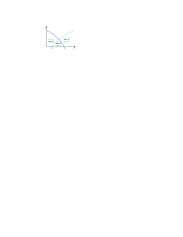
Figure 1: Schematic phase diagram on $(x,T)$-plane of the order parameters described by complex ($\psi$) and real ($\phi$) fields. $x$ represents certain adjustable parameter whose variation tunes phase transitions. $x_{1}$ and $x_{2}$ are quantum critical points of the corresponding phase transitions, respectively.

A natural question is how the ordering competition is influenced by various symmetry-breaking patterns. Moreover, the order parameter exhibits different properties in the disordered phase, ordered phase, and quantum critical region Vojta2003RPP ; Sachdev2011PT (the small region on phase diagram around quantum critical point). In the disordered phase, the order parameter has vanishing mean value, and its quantum fluctuation is not expected to be strong. In the close vicinity of quantum critical point, the mean value of order parameter still vanishes, but the quantum fluctuation becomes singular and can cause nontrivial quantum critical phenomena Sachdev1999Book . In the ordered phase, the properties of order parameter is heavily affected by the nature of broken symmetry. In the special case of continuous symmetry breaking, the amplitude fluctuation of order parameter is gapped (massive), whereas Goldstone bosonic excitation is always gapless (massless). It is thus necessary to examine whether Goldstone bosons play crucial roles in the description of ordering competition. These problems were not systematically addressed previously, which motivated us to revisit the problem of ordering competition.

In this paper, we will study these problems within an effective quantum field theory for the competition between two distinct order parameters. As aforementioned, the order competition problem is complicated and determined by the concrete symmetry-breaking pattern. Moreover, the properties may be very different in ordered and disordered phases. It is hardly possible to make a general field-theoretic analysis that applies to all cases. For concreteness, we only consider a particular case in which the system contains one complex scalar field and one real scalar field. Our focus will be on the stability of the system in the low-energy region, which is usually examined by determining the possible stable fixed points due to interactions. It would be easy to apply the same scheme to study other systems of ordering competition.

The most suitable method to address the above issues is to perform renormalization group (RG) calculations Wilson1975RMP . We will adopt the momentum-shell RG scheme Polchinski ; Shankar , which is physically intuitive and also formally simple. We first derive the RG flow equations for all the relevant parameters in the field theory, and then solve these self-consistently coupled equations numerically. Interestingly, we find the interacting system does not have any stable fixed point, which implies that the continuous phase transition are turned to first-order. Such instability is primarily driven by the quantum fluctuation of the amplitude of order parameter, rather than Goldstone boson, and the competitive interaction between distinct long-range orders.

The rest of the paper is organized as follows. We present the quantum field theory and the corresponding Feynman rules in Sec. II. RG calculations are carried out in Sec. III. We briefly discuss the physical implications of our results in Sec. IV. To better understand the consequence of ordering competition, we consider the region where two competing orders coexist homogeneously in Sec. V, and find that the originally massless Goldstone boson become massive as a direct and nontrivial consequence of ordering competition. In this case, the system also undergoes a first-order instability. In Sec. VI, we briefly summarize the results and discuss the possible extension of the work.

II Effective field theory for ordering competition

In principle, an order parameter can be a real scalar field, a complex scalar field, or a vector field. In this paper, we are mainly interested in the interplay between two distinct scalar fields. To keep a balance between generality and simplicity, we assume one of them is a complex scalar field whereas the other a real scalar field. Moreover, we consider a (2+1)-dimensional model since the ordering competition phenomena usually take place in layered superconductors. It is straightforward to generalize the analysis to other forms of order parameters and to other space-time dimensions.

The competition between two distinct order parameters can be described by the following field theory

$$\mathcal{L} = \mathcal{L}_{\psi}+\mathcal{L}_{\phi}+\mathcal{L}_{\psi\phi},$$ (1)

$$\mathcal{L}_{\psi} = \partial_{\mu}\psi^{\dagger}\partial_{\mu}\psi-\alpha|\psi|^{2}+\frac{\beta}{2}|\psi|^{4},$$ (2)

$$\mathcal{L}_{\phi} = \frac{1}{2}(\partial_{\mu}\phi)^{2}+r\phi^{2}+\frac{u}{2}\phi^{4},$$ (3)

$$\mathcal{L}_{\psi\phi} = \lambda|\psi|^{2}\phi^{2},$$ (4)

where $\mathcal{L}_{\psi}$ and $\mathcal{L}_{\phi}$ are the Ginzburg-Landau model for order parameters $\psi$ and $\phi$, respectively. $\mathcal{L}_{\psi\phi}$ represents the interaction between $\psi$ and $\phi$. Such interaction is repulsive or competitive if the coupling constant $\lambda$ is chosen to be positive. The mass parameters $\alpha$ and $r$ tune the phase transitions that lead to finite mean values of $\psi$ and $\phi$, respectively. For example, if $\alpha<0$, the free energy of $\psi$ exhibits its minimum at $\langle\psi\rangle=0$, which implies the system is in the disordered phase. If $\alpha>0$, the minimum of free energy of $\psi$ is located at a finite $\langle\psi\rangle$, so the system is in the ordered phase. It is therefore clear that $\alpha=0$ represents the zero temperature quantum critical point that separates disordered and ordered phases, corresponding to $x_{1}$ in the phase diagram Fig. 1. Analogously, $r=0$ is the quantum critical point for order parameter $\phi$, represented by $x_{2}$ in Fig. 1. In this paper, we assume that $\alpha>0$ and $r>0$. In addition, $\beta$ and $u$ are both positive according to the standard theory of continuous phase transition.

Let us assume that $\psi$ is a complex scalar field, which may be the order parameter of superfluidity, superconductivity, or antiferromagnetism. In the vicinity of quantum critical point $x_{2}$, the field $\psi$ acquires a finite vacuum expectation value due to vacuum degeneracy, i.e.,

$$\langle\psi\rangle=V_{0}=\sqrt{\frac{\alpha}{\beta}}.$$ (5)

Quantum fluctuation of $\psi$ is known to be strong at zero temperature, especially in the nearby of quantum critical point. The fluctuation of $\psi$ around its mean value can be described by introducing two new fields $h$ and $\eta$ Kleinert2003NPB ,

$$\psi=V_{0}+\frac{1}{\sqrt{2}}(h+i\eta),$$ (6)

where

$$\langle h\rangle=\langle\eta\rangle=0.$$ (7)

In previous analysis of ordering competition, the influence of quantum fluctuation of order parameter in the ordered phase is not carefully analyzed, and it is unclear whether massless Goldstone boson plays an important role. By employing the field parametrization Eq. (6), we are allowed to separate the contributions of amplitude fluctuation of order parameter and Goldstone boson. In order to make the impact of Goldstone boson more transparent, we assume $\phi$ is a real scalar field that is induced by discrete symmetry breaking and therefore does not contain Goldstone boson.

Substituting Eq. (6) into Eq. (1), we are left with the following Lagrangian density

$$\mathcal{L}_{\mathrm{eff}} = \frac{1}{2}(\partial_{\mu}h)^{2}+\alpha_{h}h^{2}+\gamma_{h}h^{3}+\frac{\beta_{h}}{2}h^{4}+\frac{1}{2}(\partial_{\mu}\eta)^{2}$$ (8)

$$+\frac{\beta_{\eta}}{2}\eta^{4}+\frac{1}{2}(\partial_{\mu}\phi)^{2}+\alpha_{\phi}\phi^{2}+\frac{\beta_{\phi}}{2}\phi^{4}+\gamma_{\eta h}\eta^{2}h$$

$$+\gamma_{\phi h}\phi^{2}h+\lambda_{\eta h}h^{2}\eta^{2}+\lambda_{h\phi}h^{2}\phi^{2}+\lambda_{\eta\phi}\eta^{2}\phi^{2},$$

where the new parameters are defined as

$$\alpha_{h} = \alpha,\,\,\,\,\,\,\alpha_{\phi}=\frac{\lambda\alpha}{\beta}+r,$$ (9)

$$\beta_{h} = \frac{\beta}{4},\,\,\,\beta_{\eta}=\frac{\beta}{4},\,\,\,\beta_{\phi}=u,$$ (10)

$$\gamma_{h} = \frac{\sqrt{2\alpha\beta}}{2},\gamma_{\eta h}=\frac{\sqrt{2\alpha\beta}}{2},\gamma_{\phi h}=\lambda\sqrt{\frac{2\alpha}{\beta}},$$ (11)

$$\lambda_{\eta h} = \frac{\beta}{4},\,\,\,\lambda_{h\phi}=\frac{\lambda}{2},\,\,\,\lambda_{\eta\phi}=\frac{\lambda}{2}.$$ (12)

From Eq. (8), it is easy to extract the free propagators of fields $h$, $\eta$, and $\phi$, namely

$$G_{h}(k) = \frac{1}{k^{2}+2\alpha_{h}},$$ (13)

$$G_{\eta}(k) = \frac{1}{k^{2}},$$ (14)

$$G_{\phi}(k) = \frac{1}{k^{2}+2\alpha_{\phi}}.$$ (15)

The corresponding Feynman rules for free propagators and free vertices are shown in Fig. 2 and Fig. 3. The Goldstone boson generated by continuous symmetry breaking is represented by $\eta$, whose masslessness can be readily seen from both Eq. (8) and Eq. (14). On the other hand, the amplitude fluctuation of order parameter $\psi$ is encoded in field $h$, which is massive when $x\neq x_{1}$.

Figure 2: Free propagators for (a) $h$, (b) $\eta$, and (c) $\phi$.

Figure 3: Vertices: (a) $h^{3}$; (b) $\eta^{2}h$; (c) $\phi^{2}h$; (d) $h^{4}$; (e) $h^{2}\eta^{2}$; (f) $h^{2}\phi^{2}$; (g) $\eta^{4}$; (h) $\phi^{4}$; (i) $\eta^{2}\phi^{2}$.

In many field-theoretic treatments of phase transition, especially in the context of condensed matter systems, the amplitude fluctuation of order parameter, $h$ in our case, is usually considered as unimportant and hence omitted. At the mean-field level, this approximation is expected to perfectly valid. However, at zero temperature, the quantum fluctuation of $h$ is important and has unnegligible effect, which makes the mean-field treatment unreliable. This effect becomes more and more significant as one approaches the quantum critical point, where the quantum fluctuation of order parameter is indeed singular. As will be shown below, the amplitude fluctuation $h$ and its coupling with competing order is able to drive an instability of the system. In Ref. Kleinert2003NPB , Kleinert and Nogueira investigated the interaction between a superconducting order parameter and an abelian gauge field, where the field parametrization Eq. (6) of complex order parameter was adopted, and obtained an infrared-stable fixed point by means of RG method. It is also interesting to notice that, a recent work Benfatto studied the impact of amplitude fluctuation (Higgs mode) in a system with coexisting superconducting and charge-density-wave orders, and revealed important observable effects of amplitude fluctuation.

III Renormalization group analysis

There are several RG schemes available in the literature, ranging from Wilson’s original momentum-shell scheme Wilson1975RMP to the more complicated function RG scheme Wetterich ; Metzner2012RMP . Here we adopt the momentum-shell scheme Polchinski ; Shankar .

III.1 Effective action

The essence of RG analysis is to integrate out high energy (small scale) degrees of freedom and select out low energy (large scale) degrees of freedom. It is therefore necessary to express the action of field operators $h$, $\eta$, and $\phi$ as integrals over momenta and energies. Formally, we have

$$S = S_{h}+S_{\eta}+S_{\phi}+S_{\eta^{2}h}+S_{\phi^{2}h}+S_{h^{2}\eta^{2}}$$ (16)

$$+S_{h^{2}\phi^{2}}+S_{\eta^{2}\phi^{2}},$$

where

$$S_{h} = \frac{1}{2}\int\frac{d^{2}\mathbf{k}d\omega}{(2\pi)^{3}}\left(2\alpha_{h}+\mathbf{k}^{2}+\omega^{2}\right)h^{2}$$ (17)

$$+\gamma_{h}\int\prod^{3}_{m=1}\frac{d^{2}\mathbf{k}_{m}d\omega_{m}}{(2\pi)^{3}}\Delta(m)h^{3}$$

$$+\frac{\beta_{h}}{2}\int\prod^{4}_{m=1}\frac{d^{2}\mathbf{k}_{m}d\omega_{m}}{(2\pi)^{3}}\Delta(m)h^{4},$$

$$S_{\eta} = \frac{1}{2}\int\frac{d^{2}\mathbf{k}d\omega}{(2\pi)^{3}}\left(\mathbf{k}^{2}+\omega^{2}\right)\eta^{2}$$ (18)

$$+\frac{\beta_{\eta}}{2}\int\prod^{4}_{m=1}\frac{d^{2}\mathbf{k}_{m}d\omega_{m}}{(2\pi)^{3}}\Delta(m)\eta^{4},$$

$$S_{\phi} = \int\frac{d^{2}\mathbf{q}d\epsilon}{(2\pi)^{3}}\frac{1}{2}\left(2\alpha_{\phi}+\mathbf{q}^{2}+\epsilon^{2}\right)\phi^{2}$$ (19)

$$+\frac{\beta_{\phi}}{2}\int\prod^{4}_{m=1}\frac{d^{2}\mathbf{q}_{m}d\epsilon_{m}}{(2\pi)^{3}}\Delta(m)\phi^{4},$$

and

$$S_{\eta^{2}h} = \gamma_{\eta h}\int\prod_{i=1,2}\frac{d^{2}\mathbf{k}_{i}d\omega_{i}}{(2\pi)^{3}}\frac{d^{2}\mathbf{k^{\prime}}d\omega^{\prime}}{(2\pi)^{3}}$$ (20)

$$\times\eta(\mathbf{k}_{i},\omega_{i})h(\mathbf{k^{\prime}},\omega^{\prime})\Gamma^{(\mathbf{k},\mathbf{k^{\prime}})}_{(\omega,\omega^{\prime})},$$

$$S_{\phi^{2}h} = \gamma_{\phi h}\int\prod_{i=1,2}\frac{d^{2}\mathbf{q}_{i}d\epsilon_{i}}{(2\pi)^{3}}\frac{d^{2}\mathbf{k}d\omega}{(2\pi)^{3}}$$ (21)

$$\times\phi(\mathbf{q}_{i},\epsilon_{i})h(\mathbf{k},\omega)\Gamma^{(\mathbf{q},\mathbf{k})}_{(\epsilon,\omega)},$$

$$S_{h^{2}\eta^{2}} = \lambda_{\eta h}\int\prod_{i=1,2}\frac{d^{2}\mathbf{k}_{i}d\omega_{i}d^{2}\mathbf{k^{\prime}}_{i}d\omega^{\prime}_{i}}{(2\pi)^{6}}$$ (22)

$$\times\eta(\mathbf{k}_{i},\omega_{i})h(\mathbf{k^{\prime}}_{i},\omega^{\prime}_{i})\Xi^{(\mathbf{k},\mathbf{k^{\prime}})}_{(\omega,\omega^{\prime})},$$

$$S_{h^{2}\phi^{2}} = \lambda_{h\phi}\int\prod_{i=1,2}\frac{d^{2}\mathbf{k}_{i}d\omega_{i}d^{2}\mathbf{q}_{i}d\epsilon_{i}}{(2\pi)^{6}}$$ (23)

$$\times h(\mathbf{k}_{i},\omega_{i})\phi(\mathbf{q}_{i},\epsilon_{i})\Xi^{(\mathbf{k},\mathbf{q})}_{(\omega,\epsilon)},$$

$$S_{\eta^{2}\phi^{2}} = \lambda_{\eta\phi}\int\prod_{i=1,2}\frac{d^{2}\mathbf{k}_{i}d\omega_{i}d^{2}\mathbf{q}_{i}d\epsilon_{i}}{(2\pi)^{6}}$$ (24)

$$\times\eta(\mathbf{k}_{i},\omega_{i})\phi(\mathbf{q}_{i},\epsilon_{i})\Xi^{(\mathbf{k},\mathbf{q})}_{(\omega,\epsilon)}).$$

Here, in order to simplify notations, we have defined

$$\Delta(m) \equiv \delta^{2}\left(\sum\mathbf{k}_{m}\right)\delta\left(\sum\omega_{m}\right),$$

$$\Gamma^{(\mathbf{x},\mathbf{y})}_{(s,t)} \equiv \delta^{2}\left(\mathbf{x}_{1}+\mathbf{x}_{2}+\mathbf{y}\right)\delta\left(s_{1}+s_{2}+t\right),$$

$$\Xi^{(\mathbf{x},\mathbf{y})}_{(s,t)} \equiv \delta^{2}\left(\mathbf{x}_{1}+\mathbf{x}_{2}+\mathbf{y}_{1}+\mathbf{y}_{2}\right)\delta\left(s_{1}+s_{2}+t_{1}+t_{2}\right).$$

Since all the terms in $S$ are already written as integrals over momenta and energies, we are now ready to eliminate the modes of large momenta and high energies.

III.2 Scaling transformations

Following the formalism presented in Refs. Polchinski ; Shankar , we first make scaling transformations,

$$k_{x,y} = k^{\prime}_{x,y}e^{-l},$$ (25)

$$\omega = \omega^{\prime}e^{-l},$$ (26)

$$q_{x,y} = q^{\prime}_{x,y}e^{-l},$$ (27)

$$\epsilon = \epsilon^{\prime}e^{-l},$$ (28)

where $l$ is a running scale that goes to infinity at the lowest energy. Under these transformations, the field operators $h$, $\eta$, and $\phi$ should transform accordingly so that the free parts of actions $S_{h}$, $S_{\eta}$, and $S_{\phi}$ remain unchanged. In order words, they are defined as free fixed points under RG scaling transformations. It is easy to know from the free actions that $h$, $\eta$, and $\phi$ should be re-scaled as

$$h(\mathbf{k},\omega) = h^{\prime}(\mathbf{k^{\prime}},\omega^{\prime})e^{5l/2},$$ (29)

$$\eta(\mathbf{k},\omega) = \eta^{\prime}(\mathbf{k^{\prime}},\omega^{\prime})e^{5l/2},$$ (30)

$$\phi(\mathbf{q},\epsilon) = \phi^{\prime}(\mathbf{q^{\prime}},\epsilon^{\prime})e^{5l/2}.$$ (31)

III.3 Slow and fast modes of field operators

To proceed, we need to separate each field operator into slow mode and fast mode, i.e.,

$$h = h_{s}+h_{f},$$ (32)

$$\eta = \eta_{s}+\eta_{f},$$ (33)

$$\phi = \phi_{s}+\phi_{f}.$$ (34)

Such separation would be meaningless without specifying which modes are fast or slow. We introduce an ultraviolet cutoff $\Lambda$, which naturally exists in realistic condensed matter systems, and then rescale momenta and energy using $\Lambda$, i.e.,

$$\mathbf{k}\rightarrow\mathbf{k}/\Lambda,\hskip 7.11317pt\omega\rightarrow\omega/\Lambda.$$ (35)

In terms of new variables, we define the slow modes as

$$h_{s} = h(k)\hskip 7.11317pt\mathrm{for}\hskip 7.11317pt0<k<b,$$ (36)

$$\eta_{s} = \eta(k)\hskip 7.11317pt\mathrm{for}\hskip 7.11317pt0<k<b,$$ (37)

$$\phi_{s} = \phi(k)\hskip 7.11317pt\mathrm{for}\hskip 7.11317pt0<k<b,$$ (38)

and the fast modes as

$$h_{f} = h(k)\hskip 7.11317pt\mathrm{for}\hskip 7.11317ptb<k<1,$$ (39)

$$\eta_{f} = \eta(k)\hskip 7.11317pt\mathrm{for}\hskip 7.11317ptb<k<1,$$ (40)

$$\phi_{f} = \phi(k)\hskip 7.11317pt\mathrm{for}\hskip 7.11317ptb<k<1,$$ (41)

where

$$b=e^{-l}.$$ (42)

Figure 4: One-loop corrections to $\alpha_{h}$.

Figure 5: One-loop corrections to $\alpha_{\phi}$.

Based on the above mode separation, the whole action Eq. (16) can be decomposed into three parts: $S^{s}$ that contains only slow modes, $S^{f}$ that contains only fast modes, and $S^{sf}$ that contains both slow and fast modes. The action can be rewritten in the following form

$$S = S^{s}+S^{f}+S^{sf},$$ (43)

$$S^{s} = S^{s}_{h}+S^{s}_{\eta}+S^{s}_{\phi}+S^{s}_{\eta^{2}h}+S^{s}_{\phi^{2}h}$$ (44)

$$+S^{s}_{h^{2}\eta^{2}}+S^{s}_{h^{2}\phi^{2}}+S^{s}_{\eta^{2}\phi^{2}},$$

$$S^{f} = S^{f}_{h}+S^{f}_{\eta}+S^{f}_{\phi}+S^{f}_{\eta^{2}h}+S^{f}_{\phi^{2}h}$$ (45)

$$+S^{f}_{h^{2}\eta^{2}}+S^{f}_{h^{2}\phi^{2}}+S^{f}_{\eta^{2}\phi^{2}},$$

$$S^{sf} = S^{sf}_{h}+S^{sf}_{\eta}+S^{sf}_{\phi}+S^{sf}_{\eta h}+S^{sf}_{h\phi}+S^{sf}_{\eta\phi}.$$ (46)

More concretely, the slow/fast parts are

$$S^{s,f}_{h} = \frac{1}{2}\int\frac{d^{2}\mathbf{k}d\omega}{(2\pi)^{3}}\left(2\alpha_{h}+\mathbf{k}^{2}+\omega^{2}\right)h^{2}_{s,f}$$ (47)

$$+\gamma_{h}\int\prod^{3}_{m=1}\frac{d^{2}\mathbf{k}_{m}d\omega_{m}}{(2\pi)^{3}}\Delta(m)h^{3}_{s,f}$$

$$+\frac{\beta_{h}}{2}\int\prod^{4}_{m=1}\frac{d^{2}\mathbf{k}_{m}d\omega_{m}}{(2\pi)^{3}}\Delta(m)h^{4}_{s,f},$$

$$S^{s,f}_{\eta} = \frac{1}{2}\int\frac{d^{2}\mathbf{k}d\omega}{(2\pi)^{3}}\left(\mathbf{k}^{2}+\omega^{2}\right)\eta^{2}_{s,f}$$ (48)

$$+\frac{\beta_{\eta}}{2}\int\prod^{4}_{m=1}\frac{d^{2}\mathbf{k}_{m}d\omega_{m}}{(2\pi)^{3}}\Delta(m)\eta^{4}_{s,f},$$

$$S^{s,f}_{\phi} = \frac{1}{2}\int\frac{d^{2}\mathbf{q}d\epsilon}{(2\pi)^{3}}\left(2\alpha_{\phi}+\mathbf{q}^{2}+\epsilon^{2}\right)\phi^{2}_{s,f}$$ (49)

$$+\frac{\beta_{\phi}}{2}\int\prod^{4}_{m=1}\frac{d^{2}\mathbf{q}_{m}d\epsilon_{m}}{(2\pi)^{3}}\Delta(m)\phi^{4}_{s,f},$$

$$S^{s,f}_{\eta^{2}h} = \gamma_{\eta h}\int\prod_{i=1,2}\frac{d^{2}\mathbf{k}_{i}d\omega_{i}}{(2\pi)^{3}}\frac{d^{2}\mathbf{k^{\prime}}d\omega^{\prime}}{(2\pi)^{3}}$$ (50)

$$\times\eta_{s,f}(\mathbf{k}_{i},\omega_{i})h_{s,f}(\mathbf{k^{\prime}},\omega^{\prime})\Gamma^{(\mathbf{k},\mathbf{k^{\prime}})}_{(\omega,\omega^{\prime})},$$

$$S^{s,f}_{\phi^{2}h} = \gamma_{\phi h}\int\prod_{i=1,2}\frac{d^{2}\mathbf{q}_{i}d\epsilon_{i}}{(2\pi)^{3}}\frac{d^{2}\mathbf{k}d\omega}{(2\pi)^{3}}$$ (51)

$$\times\phi_{s,f}(\mathbf{q}_{i},\epsilon_{i})h_{s,f}(\mathbf{k},\omega)\Gamma^{(\mathbf{q},\mathbf{k})}_{(\epsilon,\omega)},$$

$$S^{s,f}_{h^{2}\eta^{2}} = \lambda_{\eta h}\int\prod_{i=1,2}\frac{d^{2}\mathbf{k}_{i}d\omega_{i}}{(2\pi)^{3}}\frac{d^{2}\mathbf{k^{\prime}}_{i}d\omega^{\prime}_{i}}{(2\pi)^{3}}$$ (52)

$$\times\eta_{s,f}(\mathbf{k}_{i},\omega_{i})h_{s,f}(\mathbf{k^{\prime}}_{i},\omega^{\prime}_{i})\Xi^{(\mathbf{k},\mathbf{k^{\prime}})}_{(\omega,\omega^{\prime})},$$

$$S^{s,f}_{h^{2}\phi^{2}} = \lambda_{h\phi}\int\prod_{i=1,2}\frac{d^{2}\mathbf{k}_{i}d\omega_{i}}{(2\pi)^{3}}\frac{d^{2}\mathbf{q}_{i}d\epsilon_{i}}{(2\pi)^{3}}$$ (53)

$$\times h_{s,f}(\mathbf{k}_{i},\omega_{i})\phi_{s,f}(\mathbf{q}_{i},\epsilon_{i})\Xi^{(\mathbf{k},\mathbf{q})}_{(\omega,\epsilon)},$$

$$S^{s,f}_{\eta^{2}\phi^{2}} = \lambda_{\eta\phi}\int\prod_{i=1,2}\frac{d^{2}\mathbf{k}_{i}d\omega_{i}}{(2\pi)^{3}}\frac{d^{2}\mathbf{q}_{i}d\epsilon_{i}}{(2\pi)^{3}}$$ (54)

$$\times\eta_{s,f}(\mathbf{k}_{i},\omega_{i})\phi_{s,f}(\mathbf{q}_{i},\epsilon_{i})\Xi^{(\mathbf{k},\mathbf{q})}_{(\omega,\epsilon)};$$

and the slow-fast mixing terms are

$$S^{sf}_{h} = 3\gamma_{h}\int\prod^{3}_{m=1}\frac{d^{2}\mathbf{k}_{m}d\omega_{m}}{(2\pi)^{3}}\Delta(m)\left(h_{s}h_{f}h_{f}+h_{s}h_{s}h_{f}\right)$$ (55)

$$+3\beta_{h}\int\prod^{4}_{m=1}\frac{d^{2}\mathbf{k}_{m}d\omega_{m}}{(2\pi)^{3}}\Delta(m)h_{s}h_{s}h_{f}h_{f},$$

$$S^{sf}_{\eta} = 3\beta_{\eta}\int\prod^{4}_{m=1}\frac{d^{2}\mathbf{k}_{m}d\omega_{m}}{(2\pi)^{3}}\Delta(m)\eta_{s}\eta_{s}\eta_{f}\eta_{f},$$ (56)

$$S^{sf}_{\phi} = 3\beta_{\phi}\int\prod^{4}_{m=1}\frac{d^{2}\mathbf{q}_{m}d\epsilon_{m}}{(2\pi)^{3}}\Delta(m)\phi_{s}\phi_{s}\phi_{f}\phi_{f},$$ (57)

and

$$S^{sf}_{\eta h} = \int\prod_{i=1,2}\frac{d^{2}\mathbf{k}_{i}d\omega_{i}}{(2\pi)^{3}}\frac{d^{2}\mathbf{k^{\prime}}d\omega^{\prime}}{(2\pi)^{3}}\Bigl{\{}\gamma_{\eta h}\Bigl{[}\eta_{s}(\mathbf{k}_{i},\omega_{i})h_{f}(\mathbf{k^{\prime}},\omega^{\prime})+\eta_{f}(\mathbf{k}_{i},\omega_{i})h_{s}(\mathbf{k^{\prime}},\omega^{\prime})\Bigr{]}$$ (58)

$$+2\gamma_{\eta h}\eta_{s}(\mathbf{k}_{1},\omega_{1})\eta_{f}(\mathbf{k}_{2},\omega_{2})h_{f}(\mathbf{k^{\prime}},\omega^{\prime})\Bigr{\}}\Gamma^{(\mathbf{k},\mathbf{k^{\prime}})}_{(\omega,\omega^{\prime})}+\lambda_{\eta h}\int\prod_{i=1,2}\frac{d^{2}\mathbf{k}_{i}d\omega_{i}}{(2\pi)^{3}}\frac{d^{2}\mathbf{k^{\prime}}_{i}d\omega^{\prime}_{i}}{(2\pi)^{3}}$$

$$\times\Bigl{[}\eta_{s}(\mathbf{k}_{i},\omega_{i})h_{f}(\mathbf{k^{\prime}}_{i},\omega^{\prime}_{i})+\eta_{f}(\mathbf{k}_{i},\omega_{i})h_{s}(\mathbf{k^{\prime}}_{i},\omega^{\prime}_{i})\Bigr{]}\Xi^{(\mathbf{k},\mathbf{k^{\prime}})}_{(\omega,\omega^{\prime})}+4\lambda_{\eta h}\int\prod_{i=1,2}\frac{d^{2}\mathbf{k}_{i}d\omega_{i}}{(2\pi)^{3}}\frac{d^{2}\mathbf{k^{\prime}}_{i}d\omega^{\prime}_{i}}{(2\pi)^{3}}$$

$$\times\eta_{s}(\mathbf{k}_{1},\omega_{1})\eta_{f}(\mathbf{k}_{2},\omega_{2})h_{s}(\mathbf{k^{\prime}}_{1},\omega^{\prime}_{1})h_{f}(\mathbf{k^{\prime}}_{2},\omega^{\prime}_{2})\Xi^{(\mathbf{k},\mathbf{k^{\prime}})}_{(\omega,\omega^{\prime})},$$

$$S^{sf}_{h\phi} = \int\prod_{i=1,2}\frac{d^{2}\mathbf{q}_{i}d\epsilon_{i}}{(2\pi)^{3}}\frac{d^{2}\mathbf{k}d\omega}{(2\pi)^{3}}\Bigr{\{}\gamma_{\phi h}\Bigl{[}\phi_{s}(\mathbf{q}_{i},\epsilon_{i})h_{f}(\mathbf{k},\omega)+\phi_{f}(\mathbf{q}_{i},\epsilon_{i})h_{s}(\mathbf{k},\omega)\Bigr{]}$$ (59)

$$+2\gamma_{\phi h}\phi_{s}(\mathbf{q}_{1},\epsilon_{1})\phi_{f}(\mathbf{q}_{2},\epsilon_{2})h_{f}(\mathbf{k},\omega)\Bigr{\}}\Gamma^{(\mathbf{k},\mathbf{q})}_{(\epsilon,\omega)}+\lambda_{h\phi}\int\prod_{i=1,2}\frac{d^{2}\mathbf{q}_{i}d\epsilon_{i}}{(2\pi)^{3}}\frac{d^{2}\mathbf{k}d\omega}{(2\pi)^{3}}$$

$$\times\Bigl{[}h_{s}(\mathbf{k}_{i},\omega_{i})\phi_{f}(\mathbf{q}_{i},\epsilon_{i})+h_{f}(\mathbf{k}_{i},\omega_{i})\phi_{s}(\mathbf{q}_{i},\epsilon_{i})\Bigr{]}\Xi^{(\mathbf{k},\mathbf{q})}_{(\omega,\epsilon)}+4\lambda_{h\phi}\int\prod_{i=1,2}\frac{d^{2}\mathbf{q}_{i}d\epsilon_{i}}{(2\pi)^{3}}\frac{d^{2}\mathbf{k}d\omega}{(2\pi)^{3}}$$

$$\times h_{s}(\mathbf{k}_{1},\omega_{1})h_{f}(\mathbf{k}_{2},\omega_{2})\phi_{s}(\mathbf{q}_{1},\epsilon_{1})\phi_{f}(\mathbf{q}_{2},\epsilon_{2})\Xi^{(\mathbf{k},\mathbf{q})}_{(\omega,\epsilon)},$$

$$S^{sf}_{\eta\phi} = \lambda_{\eta\phi}\int\prod_{i=1,2}\frac{d^{2}\mathbf{k}_{i}d\omega_{i}}{(2\pi)^{3}}\frac{d^{2}\mathbf{q}_{i}d\epsilon_{i}}{(2\pi)^{3}}\Bigl{[}\eta_{s}(\mathbf{k}_{i},\omega_{i})\phi_{f}(\mathbf{q}_{i},\epsilon_{i})+\eta_{f}(\mathbf{k}_{i},\omega_{i})\phi_{s}(\mathbf{q}_{i},\epsilon_{i})\Bigr{]}\Xi^{(\mathbf{k},\mathbf{q})}_{(\omega,\epsilon)}$$ (60)

$$+4\lambda_{\eta\phi}\int\prod_{i=1,2}\frac{d^{2}\mathbf{k}_{i}d\omega_{i}}{(2\pi)^{3}}\frac{d^{2}\mathbf{q}_{i}d\epsilon_{i}}{(2\pi)^{3}}\eta_{s}(\mathbf{k}_{1},\omega_{1})\eta_{f}(\mathbf{k}_{2},\omega_{2})\phi_{s}(\mathbf{q}_{1},\epsilon_{1})\phi_{f}(\mathbf{q}_{2},\epsilon_{2})\Xi^{(\mathbf{k},\mathbf{q})}_{(\omega,\epsilon)}.$$

After carrying out the above mode decomposition, we can now write the partition function as

$$Z = \int\mathcal{D}h_{s}\mathcal{D}\eta_{s}\mathcal{D}\phi_{s}\mathcal{D}h_{f}\mathcal{D}\eta_{f}\mathcal{D}\phi_{f}$$ (61)

$$\times\exp\left({S^{s}+S^{f}+S^{sf}}\right).$$

We then integrate over $\eta^{f}$, $h^{f}$, and $\phi^{f}$, and have

$$Z = \int\mathcal{D}h_{s}\mathcal{D}\eta_{s}\mathcal{D}\phi_{s}\mathrm{exp}\left(S^{\prime s}_{h}+S^{\prime s}_{\eta}+S^{\prime s}_{\phi}+S^{\prime s}_{\eta^{2}h}\right.$$ (62)

$$\left.+S^{\prime s}_{\phi^{2}h}+S^{\prime s}_{h^{2}\eta^{2}}+S^{\prime s}_{h^{2}\phi^{2}}+S^{\prime s}_{\eta^{2}\phi^{2}}\right)$$

$$\equiv \int\mathcal{D}h_{s}\mathcal{D}\eta_{s}\mathcal{D}\phi_{s}\exp{\left(S^{\prime}_{\mathrm{eff}}\right)}.$$

The next step is to integrate over all the fast modes, followed by scaling transformations. Then an effective action will be obtained. The functional integration can be performed by using the standard perturbation expansion, with the help of the following identity Shankar

$$\exp\left(-S_{\mathrm{eff}}\right)=\exp\left(-\langle S_{c}\rangle_{f}+\frac{1}{2}\langle S^{2}_{c}\rangle_{f}\right),$$ (63)

where $S^{2}_{c}$ corresponds to the connected average. In the next subsection, we will calculate RG equations up to one-loop level in powers of small coupling parameters.

III.4 One-loop corrections

All the one-loop correction diagrams are plotted in Figs. 4 - 14. As depicted in Fig. 4, there are six one-loop diagrams contributing to the renormalization of $\alpha_{h}$. One should calculate them one by one so as to get the one-loop correction to $\alpha_{h}$. The contribution from diagrams presented in the first line of Fig. 4 is

Figure 6: One-loop corrections to $\gamma_{h}$.

Figure 7: One-loop corrections to $\gamma_{\eta h}$.

Figure 8: One-loop corrections to $\gamma_{\phi h}$.

Figure 9: One-loop corrections to $\beta_{h}$.

Figure 10: One-loop corrections to $\beta_{\eta}$.

Figure 11: One-loop corrections to $\beta_{\phi}$.

Figure 12: One-loop corrections to $\lambda_{\eta h}$.

Figure 13: One-loop corrections to $\lambda_{h\phi}$.

Figure 14: One-loop corrections to $\lambda_{\eta\phi}$.

$$\Delta S^{\alpha_{h}}_{1} = \int^{b}\frac{d^{3}q}{(2\pi)^{3}}h_{s}(q)h_{s}(-q)\left\{\int^{1}_{b}\frac{d^{3}q^{\prime}}{(2\pi)^{3}}\left[-(3\gamma_{h})^{2}G_{h}(q^{\prime})G_{h}(q^{\prime})-\gamma^{2}_{\eta h}G_{\eta}(q^{\prime})G_{\eta}(q^{\prime})-\gamma^{2}_{\phi h}G_{\phi}(q^{\prime})G_{\phi}(q^{\prime})\right]\right\}$$ (64)

$$\approx \int^{b}\frac{d^{3}q}{(2\pi)^{3}}h_{s}(q)h_{s}(-q)\left[-\frac{(3\gamma_{h})^{2}}{2\pi^{2}}\int^{1}_{b}dq^{\prime}\left(\frac{1}{q^{\prime 2}}-\frac{4\alpha_{h}}{q^{\prime 4}}\right)-\frac{\gamma^{2}_{\eta h}}{2\pi^{2}}\int^{1}_{b}\frac{dq^{\prime}}{q^{\prime 2}}-\frac{\gamma^{2}_{\phi h}}{2\pi^{2}}\int^{1}_{b}dq^{\prime}\left(\frac{1}{q^{\prime 2}}-\frac{4\alpha_{\phi}}{q^{\prime 4}}\right)\right]$$

$$\approx \int^{b}\frac{d^{3}q}{(2\pi)^{3}}h_{s}(q)h_{s}(-q)\left[-\frac{(3\gamma_{h})^{2}}{2\pi^{2}}\left(1-4\alpha_{h}\right)(-\ln b)-\frac{\gamma^{2}_{\eta h}}{2\pi^{2}}(-\ln b)-\frac{\gamma^{2}_{\phi h}}{2\pi^{2}}\left(1-4\alpha_{\phi}\right)(-\ln b)\right]$$

$$= -\int^{b}\frac{d^{3}q}{(2\pi)^{3}}h_{s}(q)h_{s}(-q)\frac{1}{2\pi^{2}}\left[9\gamma^{2}_{h}(1-4\alpha_{h})+\gamma^{2}_{\eta h}+\gamma^{2}_{\phi h}(1-4\alpha_{\phi})\right]l.$$

Summing the diagrams in the second line of Fig. 4 gives rise to

$$\Delta S^{\alpha_{h}}_{2} = \int^{b}\frac{d^{3}q}{(2\pi)^{3}}h_{s}(q)h_{s}(-q)\frac{1}{2\pi^{2}}\left[3\beta_{h}(1-2\alpha_{h})+\lambda_{h\phi}(1-2\alpha_{\phi})+\lambda_{\eta h}\right]l.$$ (65)

The total one-loop correction to $\alpha_{h}$ is given by summing the above contributions, namely

$$\Delta S^{\alpha_{h}}\!\!\! = \!\!\!\Delta S^{\alpha_{h}}_{1}+\Delta S^{\alpha_{h}}_{2}$$ (66)

$$= \!\!\!\int^{b}\frac{d^{3}q}{(2\pi)^{3}}h_{s}(q)h_{s}(-q)$$

$$\!\!\!\times\frac{1}{2\pi^{2}}\left[-9\gamma^{2}_{h}(1-4\alpha_{h})-\gamma^{2}_{\eta h}-\gamma^{2}_{\phi h}(1-4\alpha_{\phi})\right.$$

$$\!\!\!\left.+3\beta_{h}(1-2\alpha_{h})+\lambda_{h\phi}(1-2\alpha_{\phi})+\lambda_{\eta h}\right]l.$$

By combing the one-loop correction (66) and the free term proportional to $\alpha_{h}$, listed in Eq. (17), we derive the RG equation of $\alpha_{h}$ after integrating fast modes and making scaling transformations,

$$\frac{d\alpha_{h}}{dl} = 2\alpha_{h}-\frac{1}{4\pi^{2}}\Bigl{[}9\gamma^{2}_{h}(1-4\alpha_{h})+\gamma^{2}_{\phi h}(1-4\alpha_{\phi})+\gamma^{2}_{\eta h}$$ (67)

$$-\lambda_{\eta h}+3\beta_{h}(2\alpha_{h}-1)+\lambda_{h\phi}(2\alpha_{\phi}-1)\Bigr{]},$$

By paralleling the above calculations, we can obtain the corrections from other diagrams. Here, we only list the results by assigning $\Delta^{n}_{m}\equiv\delta^{3}\left(\sum^{n}_{m=1}q_{m}\right)$,

$$\Delta S^{\alpha_{\phi}}\!\!\! = \!\!\!\int^{b}\frac{d^{3}q}{(2\pi)^{3}}\phi_{s}(q)\phi_{s}(-q)$$ (68)

$$\!\!\!\times\frac{1}{2\pi^{2}}\Bigl{\{}-2\gamma^{2}_{\phi h}[1-2(\alpha_{\phi}+\alpha_{h})]+(\lambda_{\eta\phi}+\lambda_{h\phi}$$

$$\!\!\!+3\beta_{\phi})-2(\alpha_{h}\lambda_{h\phi}+3\alpha_{\phi}\beta_{\phi})\Bigr{\}}l,$$

$$\Delta S^{\gamma_{h}}\!\!\! = \!\!\!\int^{b}\prod^{3}_{m=1}\frac{d^{3}q_{m}}{(2\pi)^{3}}h_{s}(q_{m})$$ (69)

$$\!\!\!\times\frac{\Delta^{3}_{m}}{2\pi^{2}}\Bigl{[}-36\gamma^{3}_{h}(1-6\alpha_{h})+9\beta_{h}\gamma_{h}(4\alpha_{h}-1)$$

$$\!\!\!+\lambda_{h\phi}\gamma_{\phi h}(4\alpha_{\phi}-1)-\lambda_{\eta h}\gamma_{\eta h}\Bigr{]}l,$$

$$\Delta S^{\gamma_{\eta h}}\!\!\! = \!\!\!\int^{b}\prod^{3}_{m=1}\frac{d^{3}q_{m}}{(2\pi)^{3}}\eta_{s}(q_{1})\eta_{s}(q_{2})h_{s}(q_{3})$$ (70)

$$\!\!\!\times\frac{\Delta^{3}_{m}}{2\pi^{2}}\Bigl{\{}-\gamma_{\eta h}\Bigl{[}4\gamma^{2}_{\eta h}\left(1-2\alpha_{h}\right)+3\beta_{\eta}\Bigr{]}+3\lambda_{\eta h}$$

$$\!\!\!\times\gamma_{h}(4\alpha_{h}-1)+\lambda_{\eta\phi}\gamma_{\phi h}(4\alpha_{\phi}-1)\Bigr{\}}l,$$

$$\Delta S^{\gamma_{\phi h}}\!\!\! = \!\!\!\int^{b}\prod^{4}_{m=1}\frac{d^{3}q_{m}}{(2\pi)^{3}}\phi_{s}(q_{1})\phi_{s}(q_{2})h_{s}(q_{3})$$ (71)

$$\!\!\!\times\frac{\Delta^{4}_{m}}{2\pi^{2}}\Bigl{\{}-4\gamma^{3}_{\phi h}[1-2(2\alpha_{\phi}+\alpha_{h})]$$

$$\!\!\!+12(\alpha_{h}\lambda_{h\phi}\gamma_{h}+\alpha_{\phi}\beta_{\phi}\gamma_{\phi h})$$

$$\!\!\!-3(\lambda_{h\phi}\gamma_{h}+\beta_{\phi}\gamma_{\phi h})-\lambda_{\eta\phi}\gamma_{\eta h}\Bigr{\}}l,$$

$$\Delta S^{\beta_{h}}\!\!\! = \!\!\!\int^{b}\prod^{3}_{m=1}\frac{d^{3}q_{m}}{(2\pi)^{3}}h_{s}(q_{1})h_{s}(q_{2})h_{s}(q_{3})h_{s}(q_{4})$$ (72)

$$\!\!\!\times\frac{\Delta^{4}_{m}}{2\pi^{2}}\Bigl{[}-108\beta_{h}\gamma^{2}_{h}(1-6\alpha_{h})-9\beta^{2}_{h}-\lambda^{2}_{\eta h}$$

$$\!\!\!-\lambda^{2}_{h\phi}+4(9\alpha_{h}\beta^{2}_{h}+\alpha_{\phi}\lambda^{2}_{h\phi})\Bigr{]}l,$$

$$\Delta S^{\beta_{\eta}}\!\!\! = \!\!\!\int^{b}\prod^{4}_{m=1}\frac{d^{3}q_{m}}{(2\pi)^{3}}\eta_{s}(q_{1})\eta_{s}(q_{2})\eta_{s}(q_{3})\eta_{s}(q_{4})$$ (73)

$$\!\!\!\times\frac{\Delta^{4}_{m}}{2\pi^{2}}\Bigl{[}-12\beta_{\eta}\gamma^{2}_{\eta h}(1-2\alpha_{h})-9\beta^{2}_{\eta}-\lambda^{2}_{\eta h}$$

$$\!\!\!-\lambda^{2}_{\eta\phi}+4(\alpha_{h}\lambda^{2}_{\eta h}+\alpha_{\phi}\lambda^{2}_{\eta\phi})\Bigr{]}l,$$

$$\Delta S^{\beta_{\phi}}\!\!\! = \!\!\!\int^{b}\prod^{4}_{m=1}\frac{d^{3}q_{m}}{(2\pi)^{3}}\phi_{s}(q_{1})\phi_{s}(q_{2})\phi_{s}(q_{3})\phi_{s}(q_{4})$$ (74)

$$\!\!\!\times\frac{\Delta^{4}_{m}}{2\pi^{2}}\Bigl{\{}-12\beta_{\phi}\gamma^{2}_{\phi h}[1-2(2\alpha_{\phi}+\alpha_{h})]-9\beta^{2}_{\phi}$$

$$\!\!\!-\lambda^{2}_{h\phi}-\lambda^{2}_{\eta\phi}+4(9\alpha_{\phi}\beta^{2}_{\phi}+\alpha_{h}\lambda^{2}_{h\phi})\Bigr{\}}l,$$

$$\Delta S^{\lambda_{\eta h}}\!\!\! = \!\!\!\int^{b}\prod^{4}_{m=1}\frac{d^{3}q_{m}}{(2\pi)^{3}}\eta_{s}(q_{1})\eta_{s}(q_{2})h_{s}(q_{3})h_{s}(q_{4})$$ (75)

$$\!\!\!\times\frac{\Delta^{4}_{m}}{2\pi^{2}}\Bigl{[}-36\lambda_{\eta h}\gamma^{2}_{h}(1-6\alpha_{h})-4\lambda_{\eta h}$$

$$\!\!\!\times\gamma^{2}_{\eta h}(1-2\alpha_{h})+4(3\alpha_{h}\lambda_{\eta h}\beta_{h}+\alpha_{\phi}$$

$$\!\!\!\times\lambda_{\eta\phi}\lambda_{h\phi}+4\alpha_{h}\lambda^{2}_{\eta h})-3\lambda_{\eta h}(\beta_{h}+\beta_{\eta})$$

$$\!\!\!-\lambda_{\eta\phi}\lambda_{h\phi}-8\lambda^{2}_{\eta h}\Bigr{]}l,$$

$$\Delta S^{\lambda_{h\phi}}\!\!\! = \!\!\!\int^{b}\prod^{4}_{m=1}\frac{d^{3}q_{m}}{(2\pi)^{3}}h_{s}(q_{1})h_{s}(q_{2})\phi_{s}(q_{3})\phi_{s}(q_{4})$$ (76)

$$\!\!\!\times\frac{\Delta^{4}_{m}}{2\pi^{2}}\Bigl{\{}-4\lambda_{h\phi}\gamma^{2}_{\phi h}[1-2(2\alpha_{\phi}+\alpha_{h})]$$

$$\!\!\!-36\lambda_{h\phi}\gamma^{2}_{h}(1-6\alpha_{h})+12\lambda_{h\phi}(\alpha_{h}\beta_{h}$$

$$\!\!\!+\alpha_{\phi}\beta_{\phi})+16\lambda^{2}_{h\phi}(\alpha_{h}+\alpha_{\phi})-3\lambda_{h\phi}$$

$$\!\!\!\times(\beta_{h}+\beta_{\phi})-\lambda_{\eta h}\lambda_{\eta\phi}-8\lambda^{2}_{h\phi}\Bigr{\}}l,$$

$$\Delta S^{\lambda_{\eta\phi}}\!\!\! = \!\!\!\int^{b}\prod^{4}_{m=1}\frac{d^{3}q_{m}}{(2\pi)^{3}}\eta_{s}(q_{1})\eta_{s}(q_{2})\phi_{s}(q_{3})\phi_{s}(q_{4})$$ (77)

$$\!\!\!\times\frac{\Delta^{4}_{m}}{2\pi^{2}}\Bigl{\{}-4\lambda_{\eta\phi}\gamma^{2}_{\phi h}[1-2(2\alpha_{\phi}+\alpha_{h})]$$

$$\!\!\!-4\lambda_{\eta\phi}\gamma^{2}_{\eta h}(1-2\alpha_{h})+4(\alpha_{h}\lambda_{\eta h}\lambda_{h\phi}$$

$$\!\!\!+3\alpha_{\phi}\lambda_{\eta\phi}\beta_{\phi}+4\alpha_{\phi}\lambda^{2}_{\eta\phi})-3\lambda_{\eta\phi}(\beta_{\eta}+\beta_{\phi})$$

$$\!\!\!-\lambda_{\eta h}\lambda_{h\phi}-8\lambda^{2}_{\eta\phi}\Bigr{\}}l.$$

Eqs. (66) - (77) represent one-loop corrections to all the mass and interaction terms of the effective action. Now one can add these corrections to the original action terms, and obtain an effective new action.

III.5 RG equations

Based on the above calculations, it is now straightforward to write down the coupled RG equations for all the parameters Wang2013NJP . Performing calculations that lead to Eq. (67), we have

$$\frac{d\alpha_{h}}{dl} = 2\alpha_{h}-\frac{1}{4\pi^{2}}\Bigl{[}9\gamma^{2}_{h}(1-4\alpha_{h})+\gamma^{2}_{\phi h}(1-4\alpha_{\phi})+\gamma^{2}_{\eta h}-\lambda_{\eta h}+3\beta_{h}(2\alpha_{h}-1)+\lambda_{h\phi}(2\alpha_{\phi}-1)\Bigr{]},$$

$$\frac{d\alpha_{\phi}}{dl} = 2\alpha_{\phi}-\frac{1}{4\pi^{2}}\Bigl{\{}2\gamma^{2}_{\phi h}\Bigl{[}1-2(\alpha_{\phi}+\alpha_{h})-\lambda_{\eta\phi}\Bigr{]}+\lambda_{h\phi}(2\alpha_{h}-1)-3\beta_{\phi}(1-2\alpha_{\phi})\Bigr{\}},$$

$$\frac{d\gamma_{h}}{dl} = \frac{3}{2}\gamma_{h}+\frac{1}{2\pi^{2}}\Bigl{\{}9\gamma_{h}\Bigl{[}\beta_{h}(4\alpha_{h}-1)-4\gamma^{2}_{h}(1-6\alpha_{h})\Bigr{]}+\lambda_{h\phi}\gamma_{\phi h}(4\alpha_{\phi}-1)-\lambda_{\eta h}\gamma_{\eta h}\Bigr{\}},$$

$$\frac{d\gamma_{\eta h}}{dl} = \frac{3}{2}\gamma_{\eta h}+\frac{1}{2\pi^{2}}\Bigl{\{}3\lambda_{\eta h}\gamma_{h}(4\alpha_{h}-1)+\lambda_{\eta\phi}\gamma_{\phi h}(4\alpha_{\phi}-1)-\gamma_{\eta h}\Bigl{[}3\beta_{\eta}+4\gamma^{2}_{\eta h}(1-2\alpha_{h})\Bigr{]}\Bigr{\}},$$

$$\frac{d\gamma_{\phi h}}{dl} = \frac{3}{2}\gamma_{\phi h}+\frac{1}{2\pi^{2}}\Bigl{\{}3\lambda_{h\phi}\gamma_{h}(4\alpha_{h}-1)+3\beta_{\phi}\gamma_{\phi h}(4\alpha_{\phi}-1)-\lambda_{\eta\phi}\gamma_{\eta h}-4\gamma^{3}_{\phi h}\Bigl{[}1-2(2\alpha_{\phi}+\alpha_{h})\Bigr{]}\Bigr{\}},$$

$$\frac{d\beta_{h}}{dl} = \beta_{h}+\frac{1}{\pi^{2}}\Bigl{\{}9\beta_{h}\Bigl{[}\beta_{h}(4\alpha_{h}-1)-12\gamma^{2}_{h}(1-6\alpha_{h})\Bigr{]}+\lambda^{2}_{h\phi}(4\alpha_{\phi}-1)-\lambda^{2}_{\eta h}\Bigr{\}},$$

$$\frac{d\beta_{\eta}}{dl} = \beta_{\eta}+\frac{1}{\pi^{2}}\Bigl{\{}\lambda^{2}_{\eta\phi}(4\alpha_{\phi}-1)+\lambda^{2}_{\eta h}(4\alpha_{h}-1)-3\beta_{\eta}\Bigl{[}3\beta_{\eta}+4\gamma^{2}_{\eta h}(1-2\alpha_{h})\Bigr{]}\Bigr{\}},$$ (78)

$$\frac{d\beta_{\phi}}{dl} = \beta_{\phi}+\frac{1}{\pi^{2}}\Bigl{\{}3\beta_{\phi}\Bigl{[}12\alpha_{\phi}\beta_{\phi}-3\beta_{\phi}-4\gamma^{2}_{\phi h}\Bigl{(}1-2(2\alpha_{\phi}+\alpha_{h})\Bigr{)}\Bigr{]}+\lambda^{2}_{h\phi}(4\alpha_{h}-1)-\lambda^{2}_{\eta\phi}\Bigr{\}},$$

$$\frac{d\lambda_{\eta h}}{dl} = \lambda_{\eta h}+\frac{1}{2\pi^{2}}\Bigl{\{}\lambda_{\eta h}\Bigl{[}4\alpha_{h}(3\beta_{h}+4\lambda_{\eta h})-8\lambda_{\eta h}-3(\beta_{h}+\beta_{\eta})-36\gamma^{2}_{h}(1-6\alpha_{h})-4\gamma^{2}_{\eta h}$$

$$\times(1-2\alpha_{h})\Bigr{]}+\lambda_{\eta\phi}\lambda_{h\phi}(4\alpha_{\phi}-1)\Bigr{\}},$$

$$\frac{d\lambda_{h\phi}}{dl} = \lambda_{h\phi}+\frac{1}{2\pi^{2}}\Bigl{\{}\lambda_{h\phi}\Bigl{[}12(\alpha_{h}\beta_{h}+\alpha_{\phi}\beta_{\phi})-3(\beta_{h}+\beta_{\phi})-4\gamma^{2}_{\phi h}\Big{(}1-2(2\alpha_{\phi}+\alpha_{h})\Bigr{)}$$

$$-36\gamma^{2}_{h}(1-6\alpha_{h})+8\lambda_{h\phi}\Big{(}2(\alpha_{h}+\alpha_{\phi})-1\Bigr{)}\Bigr{]}-\lambda_{\eta h}\lambda_{\eta\phi}\Bigr{\}},$$

$$\frac{d\lambda_{\eta\phi}}{dl} = \lambda_{\eta\phi}+\frac{1}{2\pi^{2}}\Bigl{\{}\lambda_{\eta\phi}\Bigl{[}4\alpha_{\phi}(3\beta_{\phi}+4\lambda_{\eta\phi})-3(\beta_{\eta}+\beta_{\phi})-4\gamma^{2}_{\eta h}(1-2\alpha_{h})$$

$$-4\gamma^{2}_{\phi h}\Bigl{(}1-2(2\alpha_{\phi}+\alpha_{h})\Bigr{)}-8\lambda_{\eta\phi}\Bigr{]}+\lambda_{\eta h}\lambda_{h\phi}(4\alpha_{h}-1)\Bigr{\}}.$$

As mentioned in Sec. II, there are indeed only five fundamental parameters: $\alpha$, $r$, $\beta$, $u$, and $\lambda$. To obtain the running behavior of the system, we can either directly solve Eqs. (78), or solve the RG equations of fundamental parameters extracted from Eqs. (78). We have verified that these two methods lead to the same conclusion. Here we choose to adopt the second method mainly for two reasons. First, the low-energy behavior of the original action Eqs.(1-4) can be most clearly seen from the $l$-dependence of the five fundamental parameters. In addition, it is technically easier to display the detailed $l$-dependence of five parameters than eleven parameters. The RG equations for $\alpha$, $r$, $\beta$, $u$, and $\lambda$ extracted from Eq. (78) are

$$\frac{d\alpha}{dl} = 2\alpha-\frac{1}{4\pi^{2}}\left\{\alpha\beta(5-18\alpha)+\frac{\beta}{2}(3\alpha-2)+\frac{2\alpha\lambda^{2}}{\beta}\left[1-4\left(\frac{\lambda\alpha}{\beta}+r\right)\right]+\frac{\lambda}{2}\left[2\left(\frac{\lambda\alpha}{\beta}+r\right)-1\right]\right\},$$

$$\frac{dr}{dl} = 2\left(\frac{\lambda\alpha}{\beta}+r\right)-\frac{1}{4\pi^{2}}\left\{\frac{2\lambda\alpha}{\beta}\left[2(1-2\alpha)-4\left(\frac{\lambda\alpha}{\beta}+r\right)-\lambda\right]-3u\left[1-2\left(\frac{\lambda\alpha}{\beta}+r\right)\right]\right.$$

$$\left.+\frac{\lambda}{2}(2\alpha-1)\right\}+\left(\frac{\lambda\alpha}{\beta^{2}}\frac{d\beta}{dl}-\frac{\lambda}{\beta}\frac{d\alpha}{dl}-\frac{\alpha}{\beta}\frac{d\lambda}{dl}\right),$$

$$\frac{d\beta}{dl} = \beta+\frac{1}{\pi^{2}}\left\{9\beta^{2}\left[\frac{(4\alpha-1)}{4}-6\alpha(1-6\alpha)\right]+\lambda^{2}\left[4\left(\frac{\lambda\alpha}{\beta}+r\right)-1\right]-\frac{\beta^{2}}{4}\right\},$$ (79)

$$\frac{du}{dl} = u+\frac{1}{\pi^{2}}\left\{3u\left[\left(12u+\frac{32\alpha\lambda^{2}}{\beta}\right)\left(\frac{\lambda\alpha}{\beta}+r\right)-3u-\frac{8\alpha\lambda^{2}}{\beta}(1-2\alpha)\right]+\frac{\lambda^{2}}{2}(2\alpha-1)\right\},$$

$$\frac{d\lambda}{dl} = \lambda+\frac{1}{\pi^{2}}\left\{\frac{\lambda}{2}\left[4\left(3u+\frac{8\lambda^{2}\alpha}{\beta}+2\lambda\right)\left(\frac{\lambda\alpha}{\beta}+r\right)-3\left(\frac{\beta}{4}+u\right)-3\alpha\beta(5-36\alpha)\right.\right.$$

$$\left.\left.+4\left(\lambda+\frac{2\lambda^{2}\alpha}{\beta}\right)(2\alpha-1)\right]-\frac{\beta\lambda}{8}\right\}.$$

These flow equations are strongly coupled to each other. We know from RG theory that only stable fixed points can be realized in the thermodynamic limit. So the next step is to find the possible fixed point, which by definition should be unchanged under RG transformations. In the next section, we will solve these equations self-consistently.

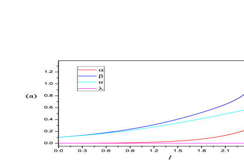
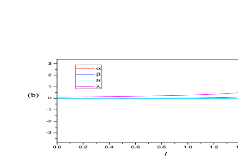
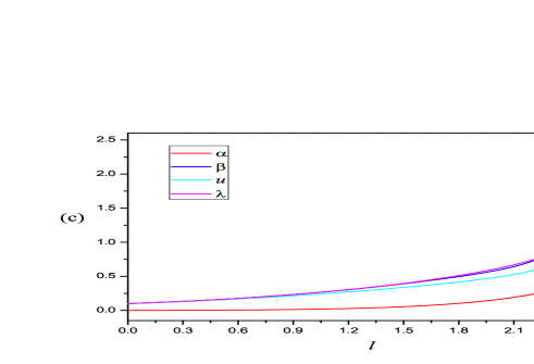
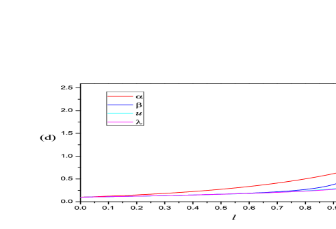
Figure 15: Initial values of dimensionless parameters: (a) $\alpha_{0}=10^{-7}$, $\beta_{0}=u_{0}=10^{-1}$, $\lambda_{0}=10^{-7}$; (b) $\alpha_{0}=10^{-7}$, $\beta_{0}=u_{0}=10^{-7}$, $\lambda_{0}=10^{-1}$; (c) $\alpha_{0}=10^{-7}$, $\beta_{0}=u_{0}=10^{-1}$, $\lambda_{0}=10^{-1}$; (d) $\alpha_{0}=10^{-1}$, $\beta_{0}=u_{0}=10^{-1}$, $\lambda_{0}=10^{-1}$.

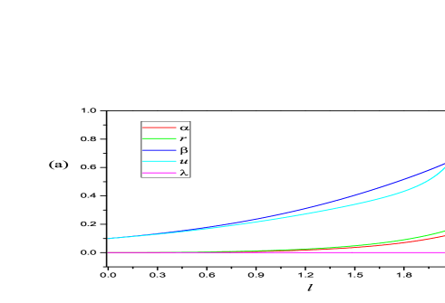
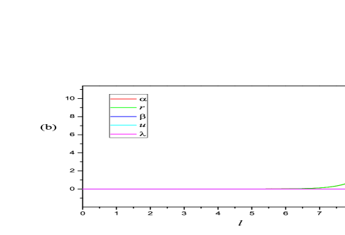
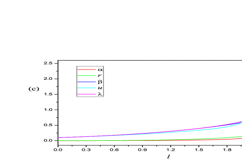
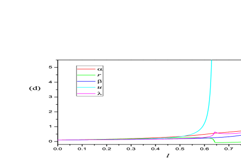
Figure 16: Initial values of dimensionless parameters: (a) $\alpha_{0}=r_{0}=10^{-7}$, $\beta_{0}=u_{0}=10^{-1}$,$\lambda_{0}=10^{-7}$; (b) $\alpha_{0}=r_{0}=10^{-7}$, $\beta_{0}=u_{0}=10^{-7}$, $\lambda_{0}=10^{-7}$; (c) $\alpha_{0}=r_{0}=10^{-7}$, $\beta_{0}=u_{0}=10^{-1}$, $\lambda_{0}=10^{-1}$; (d) $\alpha_{0}=r_{0}=10^{-1}$, $\beta_{0}=u_{0}=10^{-1}$, $\lambda_{0}=10^{-1}$.

IV RG Solutions and analysis

In this section, we study the RG equations obtained in the last section to examine whether there is any stable nontrivial fixed point in the presence of finite interactions. For this purpose, we will go through the following two steps. First, we require all the RG flow equations to vanish, leading to a set of coupled differential equations. Second, we solve these equations numerically and judge whether the solutions are stable as the running scale $l$ goes to infinity.

At the quantum critical point $x_{2}$, $r$ vanishes. By taking all the RG equations (79) to vanish, one can check that there is no physical fixed point. To confirm this result, we next solve Eqs. (79) numerically at $r=0$ and extract the explicit $l$-dependence of the other four parameters. The stability of the system is mainly determined by the behaviors of these parameters in the limit $l\rightarrow\infty$. After choosing certain initial (bare) values for $\alpha$, $\beta$, $u$, and $\lambda$, we obtain the $l$-dependence of renormalized parameters and show the results in Fig. 15. It can be seen from Fig. 15 that the qualitative conclusion does not change as the initial values of the parameters vary. In particular, the coupling parameters $\beta$, $u$, and $\lambda$ diverge rapidly as $l$ grows. These runaway behaviors clearly show the absence of any stable fixed point, and strongly suggest that the system undergoes first-order transitions  Domany_Mukamel_Fishe ; Chen_Lubensky_Nelson ; Rudnick1978PRB ; Iacobson_Amit ; Cardy1996 ; She as a consequence of ordering competition. Moreover, we find that this conclusion holds even at $r\neq 0$. In the case $r<0$, $\phi$ is also in the ordered phase, and one needs to expand $\phi$ in a form similar to Eq. (6) if the corresponding broken symmetry is also continuous. The effective field theory would become much more complicated, but the analysis can be performed in exactly the same way.

We next compare our results with previous work. The competition between two distinct order parameters was investigated within an effective (3+1)-dimensional field theory in Refs. Kosterlitz ; She . Detailed RG calculations revealed a stable fixed point, called biconical fixed point, in the system that contains a two-component order parameter and a one-component order parameter Kosterlitz . Our work differs from previous one mainly in two aspects. First, the complex order parameter is assumed to stay in the ordered phase in our work, whereas the real order parameter is very close to its quantum critical point, which allows us to carefully examine the impacts of quantum critical fluctuation of order parameter. Second, the effect of massless Goldstone boson generated by continuous symmetry breaking is explicitly incorporated.

We now wish to figure out the factor that drives the first-order transition. In particular, is the runaway behavior triggered by the massless Goldstone boson? To clarify this point, we still separate the mean value and fluctuation of order parameter in the ordered state, but choose order parameter $\psi$ to be a real scalar field which is formed by breaking a discrete symmetry. Therefore, the current system does not contain Goldstone bosons. After analogous calculations, we did not find any stable fixed point, so the phase transition is still first-order. This does not mean that Goldstone boson is unimportant. As a massless excitation (particle), Goldstone boson should have important influence on the physical properties of the system. In the present problem, however, it turns out that the amplitude fluctuation alone is significant enough to lead to runaway behavior.

V Coexisting region of two competing orders

In the previous sections, we have considered the disordered phase and the quantum critical point of long-range order $\phi$. For completeness, we now turn to the coexistence region where both order parameters $\psi$ and $\phi$ have finite mean values. In this region, $\phi$ should also be decomposed as

$$\phi=c+\sqrt{\frac{r}{u}},$$ (80)

with $\langle c\rangle=0$. Now the effective action becomes

$$\mathcal{L} = \frac{1}{2}(\partial_{\mu}h)^{2}+\alpha_{h}h^{2}+\gamma_{h}h^{3}+\frac{\beta_{h}}{2}h^{4}+\frac{1}{2}(\partial_{\mu}\eta)^{2}$$ (81)

$$+\alpha_{\eta}\eta^{2}+\frac{\beta_{\eta}}{2}\eta^{4}+\frac{1}{2}(\partial_{\mu}c)^{2}+\alpha_{c}c^{2}+\gamma_{c}c^{3}+\frac{\beta_{c}}{2}c^{4}$$

$$+\gamma_{hc}hc+\gamma_{h^{2}c}h^{2}c+\gamma_{\eta^{2}c}\eta^{2}c+\gamma_{c^{2}h}c^{2}h+\gamma_{\eta^{2}h}\eta^{2}h$$

$$+\lambda_{hc}h^{2}c^{2}+\lambda_{\eta c}\eta^{2}c^{2}+\lambda_{h\eta}h^{2}\eta^{2},$$

where

$$\alpha_{h} = \alpha+\frac{\lambda r}{2u},\,\,\alpha_{\eta}=\frac{\lambda r}{2u},\,\,\alpha_{c}=2r+\frac{\lambda\alpha}{\beta},$$ (82)

$$\beta_{c} = u,\,\,\beta_{h}=\beta_{\eta}=\frac{\beta}{4},\,\,\gamma_{h}=\gamma_{\eta^{2}h}=\frac{\sqrt{2\alpha\beta}}{2},$$ (83)

$$\gamma_{c} = 2\sqrt{ur},\,\,\gamma_{hc}=2\lambda\sqrt{\frac{2\alpha r}{\beta u}},\gamma_{c^{2}h}=\lambda\sqrt{\frac{2\alpha}{\beta}},$$ (84)

$$\gamma_{h^{2}c} = \gamma_{\eta^{2}c}=\lambda\sqrt{\frac{r}{u}},\lambda_{h\eta}=\frac{\beta}{4},\lambda_{hc}=\lambda_{\eta c}=\frac{\lambda}{2}.$$ (85)

An interesting new result is that the originally massless Goldstone boson $\eta$ acquires a finite mass due to the competitive interaction between order parameters $\psi$ and $\phi$. This mass-generating mechanism is a spectacular feature of ordering competition. Apparently, it is physically very different from Anderson-Higgs mechanism, because the latter relies crucially on the presence of spontaneous local gauge symmetry breaking which in general does not exit in our case (as long as $\psi$ does not correspond to a superconducting order parameter). The effective Goldstone boson mass vanishes at the quantum critical point $x_{2}$ since $\alpha_{\eta}\propto\lambda r\rightarrow 0$ as $r\rightarrow 0$. Furthermore, $\alpha_{\eta}$ vanishes when the competing orders decouple from each other, i.e., $\alpha_{\eta}\propto\lambda r\rightarrow 0$ as $\lambda\rightarrow 0$

Now there are no massless modes in the effective action (81). Such an action can be analyzed in exactly the same way as that presented in Sec. (III). After tedious but straightforward calculations, we obtain the RG equations of five fundamental parameters, $\alpha$, $r$, $\beta$, $u$, and $\gamma$, which will not be explicitly shown here due to the formal complicity. By carrying out numerical calculations, we show the running of these parameters in Fig. 16. It is clear that the phase transitions become first-order even in the coexisting region of competing orders.

VI Summary

In summary, we have carried out a RG analysis within a (2+1)-dimensional quantum field theory composed of two scalar fields, which is able to describe the interplay between two distinct order parameters. Different from previous treatments, we separate the quantum fluctuations of amplitude and phase of complex order parameter in the ordered state, and study their impacts on the stability of the system respectively. After deriving and analyzing the RG flow equations of all the relevant parameters, we have demonstrated that the phase transitions become first-order due to the absence of stable fixed point. We also have shown that this conclusion holds in both the ordered and disordered phases, and also at the quantum critical point.

The RG calculations presented in this paper are valid only for weak couplings. If the competitive interaction between distinct orders is not weak, one needs to invoke strong coupling approach. For instance, we might assume the scalar field has a large flavor $N$ and then perform $1/N$-expansion. In addition, when applied to study quantum phase transition, the scalar field may have a nontrivial dynamical exponent $z\neq 1$ so that its propagator is of the form $\frac{1}{k^{2}+k_{0}/k^{z-2}}$ She . In this case, the RG transformations would be different from the case with $z=1$. It is also interesting to include the interaction between scalar field and fermionic degrees of freedom, which are known to important in the theoretical description of competing orders Wang2013NJP .

VII Acknowledgments

We would like to thank Jing-Rong Wang for helpful discussions. J.W. is supported by China Postdoctoral Science Foundation under Grant No.2014M560510. G.Z.L. is supported by the National Natural Science Foundation of China under Grant No.11274286.

References

- (1) J. Zinn-Justin, Quantum Field Theory and Critical Phenomena, Clarendon Press 1989, 4th edn. Oxford University Press, Oxford (2002).
- (2) S. Sachdev, Quantum phase transitions, Cambridge University Press, Cambridge, (1999).
- (3) H. Kleinert and V. Schulte-Frohlinde, Critical Phenomena in -Theory, World Scientifc, Singapore (2001).
- (4) S. Sachdev, Science, 288, 475 (2000).
- (5) S. A. Kivelson, I. P. Bindloss, E. Fradkin, V. Oganesyan, J. M. Tranquada, A. Kapitulnik and C. Howald, Rev. Mod. Phys. 75, 1201 (2003).
- (6) M. Vojta, Adv. Phys. 58, 699 (2009).
- (7) D. P. Arovas, A. J. Berlinsky, C. Kallin and S. -C. Zhang, Phys. Rev. Lett. 79, 2871 (1997).
- (8) E. Demler, S. Sachdev and Y. Zhang, Phys. Rev. Lett. 87, 067202 (2001).
- (9) Z. Nussinov, I. Vekhter and A. V. Balatsky, Phys. Rev. B 79, 165122 (2009).
- (10) A. J. Millis, Phys. Rev. B 81, 035117 (2010).
- (11) R. M. Fernandes and J. Schmalian, Phys. Rev. B 82, 014521 (2010).
- (12) J. -H. She, J. Zaanen, A. R. Bishop and A. V. Balatsky, Phys. Rev. B 82, 165128 (2010).
- (13) D. Chowdhury, E. Berg and S. Sachdev, Phys. Rev. B 84, 205113 (2011).
- (14) C. J. Halboth and W. Metzner, Phys. Rev. Lett. 85, 5162 (2000); J. Reiss, D. Rohe, and W. Metzner, Phys. Rev. B 75, 075110 (2007).
- (15) J. Wang, A. Eberlein, and W. Metzner, Phys. Rev. B 89, 121116(R) (2014).
- (16) G. -Z. Liu, J. -R. Wang, and J. Wang, Phys. Rev. B 85, 174525 (2012).
- (17) J. Wang and G. -Z. Liu, New J. Phys. 15, 073039 (2013).
- (18) R. M. Fernandes, S. Maiti, P. Wölfle, and A. V. Chubukov, Phys. Rev. Lett. 111, 057001 (2013).
- (19) R. M. Fernandes and A. J. Millis, Phys. Rev. Lett. 111, 127001 (2013).
- (20) D. Chowdhury, B. Swingle, E. Berg, and S. Sachdev, Phys. Rev. Lett. 111, 157004 (2013).
- (21) Y. Kawaguchi and M. Ueda, Phys. Rep. 520, 253 (2012); D. M. Stamper-Kurn and M. Ueda, Rev. Mod. Phys. 85, 1191 (2013).
- (22) Q. Gu, Phys. Rev. A 68, 025601 (2003); Q. Gu, K. Bongs, and K. Sengstock, Phys. Rev. A 70, 063609 (2004); Q. Gu, arXiv: cond-mat/0512693v1 (2005).
- (23) S. S. Saxena et al., Nature (London) 406, 587 (2000); C. Pfleiderer et al., Nature (London) 412, 58 (2001); D. Aoki et al., Nature (London) 413, 613 (2001).
- (24) K. Machida and T. Ohmi, Phys. Rev. Lett. 86, 850 (2001); M. B. Walker and K. V. Samokhin, Phys. Rev. Lett. 88, 207001 (2002).
- (25) M. Vojta, Rep. Prog. Phys. 66, 2069 (2003).
- (26) S. Sachdev and B. Keimer, Phys. Today 64, 29 (2011).
- (27) K. G. Wilson, Rev. Mod. Phys. 47, 773 (1975).
- (28) J. Polchinski, arXiv:hep-th/9210046.
- (29) R. Shankar, Rev. Mod. Phys. 66, 129 (1994).
- (30) H. Kleinert and F. S. Nogueira, Nucl. Phys. B 651, 361 (2003).
- (31) T. Cea and L. Benfatto, arXiv:1407.6497.
- (32) C. Wetterich, Phys. Lett. B 301, 90 (1993); J. Berges, N. Tetradis, and C. Wetterich, Phys. Rep. 363, 223 (2002).
- (33) W. Metzner, M. Salmhofer, C. Honerkamp, V. Meden, and K. Schönhammer, Rev. Mod. Phys. 84, 299 (2012).
- (34) E. Domany, D. Mukamel, and M. E. Fisher, Phys. Rev. B 15, 5432 (1977).
- (35) J. H. Chen, T. C. Lubensky, and D. R. Nelson, Phys. Rev. B 17, 4274 (1978).
- (36) J. Rudnick, Phys. Rev. B 18, 1406 (1978).
- (37) H. H. Iacobson and D. J. Amit, Ann. Phys. 133, 57 (1981).
- (38) J. Cardy, Scaling and Renormalization in Statistical Physics, Combridge University Press, Combridge, UK, (1996).
- (39) J. M. Kosterlitz, D. R. Nelson, and M. E. Fisher, Phys. Rev. B 13, 412 (1976).