Electron-Hole Liquid in the Couple Quantum Wells

Abstract

It is shown that the homogeneous state of the spatially separated electrons and holes in the coupled quantum wells (CQW) is instable if the layer charge density is smaller than the critical value $n_{c}$ specified by the parameters of the CQW. The effect is due to the many-body Coulomb correlations which provide the positive compressibility. The instability results in the formation of the inhomogeneous system which comprises the liquid electron-hole drops.

I Introduction

The investigation of the spatially separated electrons and holes in the coupled quantum wells (CQW) is initially motivated by expecting that the electron-hole pairs forming a long-living bound state, namely exciton, can experience the Bose-Einstein condensation Lozovik . In such systems the electrons are located within one layer of the CQW while the holes, which are spatially separated from the electrons, are located in the other layer. The interest in the CQW has greatly grown in the recent years due to the increasing ability to manufacture the high quality quantum well structures in which electrons and holes are confined in the different spatial regions between which the tunneling can be made negligible Review2011 . As early as decade and a half the existence of an electron-hole condensate phase in the CQW was predicted using the variational approach Lozovik-Berman1996 .

Recently, the effect of the many-body Coulomb correlations in the CQW on the ground state of the electron-hole system is investigated in Ref. JETLET . The layers of the CQW are supposed so thin that the in-layer charge motion is a 2D one. In paperJETLET , the compressibility is found to be positive if the initial layer charge density $n<n_{c},$ the critical value $n_{c}$ being specified by the physical parameters of the CQW. The positive compressibility means the instability resulting in the formation of the inhomogeneous system which comprises the liquid electron-hole drops. Also, it was found in Ref.JETLET that the homogeneous exciton gas phase possesses the higher energy as compared to the inhomogeneous state (of the same average density) which involves the electron-hole liquid drops. Alternative scenarios for the formation of the condensed phase in the electron-hole system in the CQW are also considered in various papers, in particular in Refs. sugakov ; Wilkes ; Kuznetzova . Note that the electron-hole liquid of the same origin as in Ref.JETLET was predicted for the conventional 3D-semiconductors in keldysh1 ; rice .

The results obtained in Ref.JETLET are based on the assumption that each of the layers of the CQW is a many-valley semiconductor. Thus, the every kind of the electrons or the holes is specified by the number of the valley and the spin projection. Let the number of different kind of the electrons as well as the number of different kind of the holes $\nu\gg 1$. Two limiting situations are considered in this paper: the inter-layer separation $l\ll a_{B}/\nu$ and $l\gg a_{B}/\nu$, $a_{B}$ being the effective Bohr radius. In the first case, the electron-hole liquid drops are formed which possess the in-layer density $n_{c}\sim\nu^{3/2}$ . In the second case, $n_{c}\sim 1/l^{3/2}.$ These results are obtained using the diagrammatic approach and the following approximation is used. For any order in the Coulomb interaction, only the diagrams are held which are of the minimal order in the small parameter $1/\nu.$ In this case, the set of the diagram is that of the RPA kind. A similar approach was developed in Ref.babich to justify the formation of the electron-hole liquid drops in conventional 3D-semiconductors. Note that the standard RPA is justified for the high-density electron-hole plasma. In Refs babich ; JETLET the RPA diagram approach is based only on the assumption that the electron-hole plasma is many-component.

In the current paper we predict the instability of the uniform electron-hole system in the CQW for the case $l\ll a_{B}/\nu$ in the approximation next beyond to the RPA. For this purpose, we investigate the pole of the 4-fermion vertex function in the approximation which along with the RPA-kind diagrams takes into account the diagrams of the next order in the parameter $1/\nu.$ It is shown that the instability, connected with the pole of the vertex function, corresponds to the thermodynamical instability induced by the positive compressibility revealed in Ref. JETLET .

Strictly speaking, the result obtained is justified for the many-component system, $\nu\gg 1.$ However, comparing the result found in Ref.JETLET (obtained in the main $1/\nu$ approximation) with that found in the current paper (obtained in the next approximation in the parameter $1/\nu$) manifests that the critical concentration is insensitive to the approximation. For this reason, one can expect that the instability revealed takes place if the parameter $\nu$ is not very large.

For the sake of simplicity, the system of units is used with the effective electron (hole) charge $e=1,$ the effective electron (hole) masses $m_{e}=m_{h}=1,$ and the Planck constant $\hbar=1$. Then, the effective Bohr radius is $a_{B}=1$ and the energy is measured in the Hartree units $m_{e}e^{4}/\hbar^{2}=1$.

II The Hamiltonian and the Vertex Function

The Hamiltonian of the system is $\widehat{H}=\widehat{H}_{0}+\widehat{V},\leavevmode\nobreak\ \widehat{H}_{0}$ being the kinetic energy and $\widehat{V}$ being the Coulomb interaction. In the second quantization one has

$$\begin{array}[]{l}\widehat{H}_{0}=\sum\limits_{\alpha\sigma\mathbf{k}}\frac{k^{2}}{2}a_{\alpha\sigma}^{+}\left(\mathbf{k}\right)a_{\alpha\sigma}\left(\mathbf{k}\right);\\ \widehat{V}=\frac{1}{2S}\sum\limits_{\alpha\alpha^{\prime}\sigma\sigma^{\prime}\mathbf{kk}^{\prime}\mathbf{q}}V_{\alpha\alpha^{\prime}}\left(\left|\mathbf{q}\right|\right)a_{\alpha\sigma}^{+}\left(\mathbf{k}\right)a_{\alpha^{\prime}\sigma^{\prime}}^{+}\left(\mathbf{k}^{\prime}\right)a_{\alpha^{\prime}\sigma^{\prime}}\left(\mathbf{k}^{\prime}-\mathbf{q}\right)a_{\alpha\sigma}\left(\mathbf{k}+\mathbf{q}\right).\end{array}$$ (1)

Here $\alpha=e$ stands for the electrons, while $\alpha=h$ stands for the holes, $\sigma=1,...,\nu$ labels the kind of the electron or the hole; $a_{\alpha\sigma}^{+}\left(\mathbf{k}\right)$ and $a_{\alpha\sigma}\left(\mathbf{k}\right)$ are the creation and annihilation operators, $\mathbf{k}$ is the in-layer $2D$ momentum, and $S$ is the area of the layers. The Coulomb interaction in the momentum representation, which is assumed to be independent on the valley, reads

$$V_{\alpha\alpha^{\prime}}\left(\left|\mathbf{k}\right|\right)=\left\{\begin{array}[]{c}V=\frac{2\pi}{\left|\mathbf{k}\right|},\alpha=\alpha^{\prime};\\ V^{\prime}=-\frac{2\pi}{\left|\mathbf{k}\right|}e^{-\left|\mathbf{k}\right|l},\alpha\neq\alpha^{\prime}.\end{array}\right.$$ (2)

The Fermi momentum and the Fermi energy for the electrons and the holes are the same and are equal to $p_{F}=2\pi^{1/2}\left(n/\nu\right)^{1/2}$ and $\varepsilon_{F}=2\pi n/\nu$, respectively, $n$ being the layer concentration of the electrons or the holes. It is assumed that the temperature $T\ll\varepsilon_{F}$ and the concentration $n\ll\nu^{3}.$

Let us consider the four-fermion vertex function $\Gamma_{\alpha\sigma,\alpha^{\prime}\sigma^{\prime}}=\Gamma_{\alpha\sigma,\alpha^{\prime}\sigma^{\prime}}\left(p_{1};p_{2};k\right)$ in the Matsubara representation. The subscripts $\alpha\sigma$ and $\alpha^{\prime}\sigma^{\prime}$ label the two input ends. The two output ends are the same. The notations $p_{1}=\left(\mathbf{p}_{1},i\omega_{1}\right)$ and $p_{2}=\left(\mathbf{p}_{2},i\omega_{2}\right)$ are used which determine the input momentums $\mathbf{p}_{1}$ and $\mathbf{p}_{2}$ and the input Matsubara frequencies $\omega_{1}$ and $\omega_{2}$, while the argument $k=\left(\mathbf{k},i\varepsilon\right)$ specifies the transfer momentum $\mathbf{k}_{1}$ and the transfer frequency $\varepsilon$.

Let us introduce the concept of an irreducible diagram. A diagram is called an irreducible one if it cannot be separated into two parts linked only by one interaction line $V_{\alpha\alpha^{\prime}}\left(\left|\mathbf{k}\right|\right)$. Let $\Gamma_{\alpha\sigma,\alpha^{\prime}\sigma^{\prime}}^{\left(0\right)}$ be a set of all the irreducible diagrams which contribute into $\Gamma_{\alpha\sigma,\alpha^{\prime}\sigma^{\prime}}$. The functions $\Gamma_{\alpha\sigma,\alpha^{\prime}\sigma^{\prime}}$ and $\Gamma_{\alpha\sigma,\alpha^{\prime}\sigma^{\prime}}^{\left(0\right)}$ are connected as is shown in Fig. 1

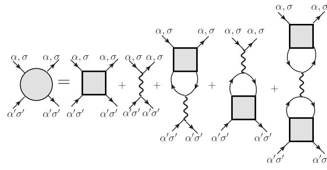
Figure 1: The exact diagrammatic expansion for the vertex function $\Gamma_{\alpha\sigma,\alpha^{\prime}\sigma^{\prime}}$ which is represented by the gray circle. The gray squares designate the irreducible vertex $\Gamma_{\alpha\sigma,\alpha^{\prime}\sigma^{\prime}}^{\left(0\right)}\leavevmode\nobreak\$which is a sum of all irreducible diagrams. The wavy lines designate the total screened Coulomb interaction $U_{\alpha a^{\prime}}\left(k\right)$ (see. Fig.2 ) The (internal) solid lines designate the total Green functions $G\left(k\right)$.

The wavy lines in the diagrams in Fig. 1 correspond to the total screened Coulomb interaction $U_{\alpha\alpha^{\prime}}=U_{\alpha\alpha^{\prime}}\left(k\right)$. This interaction is connected with the bare interaction (2) by means of the polarization operator $\Pi_{\alpha\sigma,\alpha^{\prime}\sigma}=\Pi_{\alpha\sigma,\alpha^{\prime}\sigma}(k)$ according to Fig. 2.

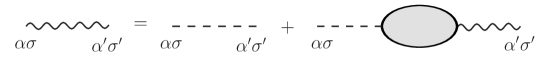
Figure 2: The exact self-consistent equation for the total screened Coulomb interaction $U_{\alpha a^{\prime}}\left(k\right)$ which is designated by the wavy line. The dashed line represents the bare Coulomb interaction $V_{\alpha a^{\prime}}\left(\mathbf{k}\right)$. The gray oval represents the polarization operator $\Pi_{\alpha\sigma a^{\prime}\sigma^{\prime}}\left(k\right).$

The system of the diagrammatic equations in Figs. 1, 2 is not complete. To proceed, let us first turn to the irreducible vertex $\Gamma_{\alpha\sigma,\alpha^{\prime}\sigma^{\prime}}^{\left(0\right)}.$ The minimal order in the interaction $U_{\alpha\alpha^{\prime}}$ for the diagrams which contribute into $\Gamma_{\alpha\sigma,\alpha^{\prime}\sigma^{\prime}}^{\left(0\right)}$ is the second order. In this case, the vertex $\Gamma_{\alpha\sigma,\alpha^{\prime}\sigma^{\prime}}^{\left(0\right)}$ designated as $\gamma_{\alpha\sigma,\alpha^{\prime}\sigma^{\prime}}$ is given by the sum of two diagrams as provided by Fig. 4

Let us consider the vertex function $\gamma_{\alpha\sigma,\alpha^{\prime}\sigma^{\prime}}$ for the momenta and frequencies which obey the limitation

$$\mid\mathbf{p}_{1}\mid,\mid\mathbf{p}_{2}\mid,\mid\mathbf{k}\mid\leq p_{F};\mid\omega_{1}\mid,\mid\omega_{2}\mid,\mid\varepsilon\mid\leq p_{F}^{2}/2.$$ (3)

As is shown in the Appendix, in this case the vertex function depends neither on the $\alpha\leavevmode\nobreak\$nor on the $\sigma,$ and $\gamma_{\alpha\sigma,\alpha^{\prime}\sigma^{\prime}}=-C/n^{2/3},$ $C$ being the factor of the order of unity, $n$ being the in-layer charge concentration. Let us then remind that the number of the valleys $\nu$ is a large parameter. For this reason, among all the irreducible diagrams of a given order in the interaction $U_{\alpha\alpha^{\prime}},$ let us hold only those which are of the minimal order in the parameter $1/\nu.$ One can convince oneself that such sequence of the main diagrams obey the diagrammatic relation in Fig. 4

Figure 3: The white square designates the irreducible vertex function calculated in the second order in the screened interaction $U_{\alpha\alpha^{\prime}}$.

Figure 4: The self-consistent diagram equation for the irreducible vertex function $\Gamma_{\alpha\sigma,\alpha^{\prime}\sigma^{\prime}}^{\left(0\right)}$ main in the parameter $\nu$.

The polarization operator $\Pi_{\alpha\sigma,\alpha^{\prime}\sigma^{\prime}}$, calculated in the same approximation as the vertex function $\Gamma_{\alpha\sigma,\alpha^{\prime}\sigma^{\prime}}^{\left(0\right)}$ in Fig. 4, is represented by the diagrams shown in Fig. 6.

Figure 5: The polarization operator $\Pi_{\alpha\alpha^{\prime}}$ calculated in the main in the parameter $\nu$ approximation. The gray square corresponds to the diagram for the $\Gamma_{\alpha\alpha^{\prime}}^{\left(0\right)}$ calculated according Fig. 4

Figure 6: The self-consistent diagrammatic relation for the vertex function $\Gamma_{\alpha\sigma,\alpha^{\prime}\sigma^{\prime}}.$

Now, the system of equations represented by the diagrams in Figs. 1-6 becomes complete what allows to obtain the self-consistent diagrammatic equation for the vertex function $\Gamma$ shown in Fig. 6.

Since the function $\gamma_{\alpha\sigma,\alpha^{\prime}\sigma^{\prime}}$ is a subscript independent, one can write $\Gamma=\Gamma_{e\sigma,e\sigma^{\prime}}=\Gamma_{h\sigma,h\sigma^{\prime}}$ and $\Gamma^{\prime}=\Gamma_{e\sigma,h\sigma^{\prime}}=\gamma_{\alpha\sigma,\alpha^{\prime}\sigma^{\prime}}.$ Then, the diagrammatic equations in Fig. 6 reads

$$\Gamma = \left(V+\gamma\right)+\left(V+\gamma\right)\Pi_{0}\Gamma+\left(V^{\prime}+\gamma\right)\Pi_{0}\Gamma^{\prime},$$ (4)

$$\Gamma^{\prime} = \left(V^{\prime}+\gamma\right)+\left(V^{\prime}+\gamma\right)\Pi_{0}\Gamma+\left(V^{\prime}+\gamma\right)\Pi_{0}\Gamma^{\prime}.$$

where the polarization operator $\Pi_{0}\left(p\right)$ is given by Eq. (15). According to Eq.(2), $V^{\prime}\left(\left|\mathbf{k}\right|\right)\approx-V\left(\left|\mathbf{k}\right|\right)+2\pi l$ if $\left|\mathbf{k}\right|l\ll 1.$ Then, it follows from (4) that

$$\Gamma \approx -\frac{1}{2\Pi_{0}}+\frac{\gamma+\pi l}{\left(1-2\left(\gamma+\pi l\right)\Pi_{0}\right)},$$ (5)

$$\Gamma^{\prime} = \frac{1}{2\Pi_{0}\left(1-2\left(\gamma+\pi l\right)\Pi_{0}\right)}.$$ (6)

The vertex functions (5) and (6) have a pole if

$$1-2\left(\gamma+\pi l\right)\Pi_{0}=0.$$ (7)

It follows from Eq.(13) and Eq.(15) that $\Pi_{0}\left(\left|\mathbf{p}\right|\rightarrow 0\right)=-\nu/2\pi.$ Since $\gamma=-C/n^{2/3}$, one obtains that the vertex functions $\Gamma_{ee},\Gamma_{eh}$ have the pole at the concentration

$$n_{c}=\left(\frac{C}{2\pi\left(1/\nu+l\right)}\right)^{3/2}.$$ (8)

Thus, for the concentration $n<n_{c}$ the uniform state of the system is unstable.

III The connection between the vertex function $\gamma\left(k\rightarrow 0\right)$ and the compressibility

Let us give a thermodynamic interpretation of the instability point given by Eq.(7). According to paper JETLET , within the RPA

$$\mu=\frac{2\pi n}{N}+2\pi nl+\mu_{corr},\leavevmode\nobreak\ \mu_{corr}=-\frac{T}{S}\sum\limits_{\mathbf{p},\omega}\left(U^{\left(0\right)}\left(p\right)-V\left(p\right)\right)G\left(p\right).$$ (9)

where the function $U^{\left(0\right)}\left(p\right)$ and the Green function $G\left(p\right)$ are given by Eqs. (14) and (13). Then, one can transform this expression as follows

$$\mu_{corr}\approx-\frac{1}{2}\int\frac{d^{2}kd\omega}{\left(2\pi\right)^{3}}\left(\frac{\left[V\left(p\right)\Pi_{0}\left(p\right)/n\right]}{1-2n\left[V\left(p\right)\Pi_{0}\left(p\right)/n\right]}-\left(V\left(p\right)\Pi_{0}\left(p\right)/n\right)\right).$$

Taking into account that the quantity $\left[V\left(p\right)\Pi_{0}\left(p\right)/n\right]$ does not depend on the concentration $n,$ one has

$$\frac{d\mu_{corr}}{dn}=-\int\frac{d^{2}kd\omega}{\left(2\pi\right)^{3}}\left(\frac{V\left(p\right)\Pi_{0}\left(p\right)/n}{\left(1-2nV\left(p\right)\Pi_{0}\left(p\right)/n\right)}\right)^{2}.$$ (10)

Comparing this result with Eq. 17 gives $d\mu_{corr}/dn=2\gamma.$ Then, it follows from (9) that

$$\frac{d\mu}{dn}=\frac{2\pi}{\nu}+2\pi l+2\gamma.$$ (11)

Thus, the instability described by the pole of the vertex function (7) corresponds to the zero of the compressibility, which means a thermodynamical instability.

IV Conclusions

It is shown that the electron-hole system in the CQW is instable if the layer charge concentration $n<n_{c}$ (see Eq. (8)). This instability is determined by the pole of the vertex function. At the same time the physical sense of this instability means just the positivity of the compressibility. Thus, if the initial homogenouse concentration $n<n_{c}$, the system transforms into inhomogeneouse state which contains the liquid electron-hole drops with the density $n_{c}.$ However, if the system with the density $n\geq n_{c}$ is created, it exists in the honogeneouse stable state.

Appendix. The vertex function $\Gamma$ in the second order in the screened interaction

As an example, let us calculate the vertex function $\gamma_{\alpha\sigma,\alpha\sigma}\left(p_{1};p_{2};k\right).$ It is assumed in this paper that the masses of the electrons and holes are the same and do not depend on the subscript $\sigma.$ Then, the vertex function $\gamma_{\alpha\sigma,\alpha\sigma}\left(p_{1};p_{2};k\right)$ does not depend on the $\sigma$ as well. It follows from Fig. 4 that

$$\gamma_{ee}=-\int\frac{d^{3}p}{\left(2\pi\right)^{3}}U_{ee}\left(p\right)U_{ee}\left(k-p\right)\left[G_{e}\left(p_{1}-p\right)\left(G_{e}\left(p_{2}+p\right)+G_{e}\left(p_{2}+k-p\right)\right)\right].$$ (12)

It is clear that the Green function $G_{e}\left(p\right)\leavevmode\nobreak\$ and the screened interaction $U_{ee}\left(p\right)$ should be substituted into (12) in the RPA. The mass operator $\Sigma_{\alpha\sigma}\left(\omega,\mathbf{p}\right)$ and the chemical potential $\mu_{\alpha}$ depend neither on the $\alpha$ nor on the $\sigma.$ The same takes place for the Green function $G_{e}\left(p\right)=G\left(p\right)=\left(i\omega+\mu-\Sigma\left(p\right)-\mathbf{p}^{2}/2\right)^{-1}.$ According to Ref. JETLET , $\mu=p_{F}^{2}/2+2\pi n/\nu+2\pi nl-cn^{1/3}$and $\Sigma_{\alpha\sigma}\left(p\right)=2\pi n/\nu+2\pi nl-cn^{1/3}$ in the RPA. Then, the Green function in the RPA reads

$$G\left(p\right)\approx\left(i\omega+p_{F}^{2}/2-\mathbf{p}^{2}/2\right)^{-1},\leavevmode\nobreak\ p_{F}=2\pi^{1/2}\left(n/\nu\right)^{1/2}.$$ (13)

If $l\ll a_{B}/\nu,$ then the interaction $U_{ee}\left(p\right)$ in the RPA readsJETLET

$$U^{\left(0\right)}\left(p\right)=\frac{V\left(p\right)}{1-2V\left(p\right)\Pi_{0}\left(p\right)}.$$ (14)

Here

$$\Pi_{0}\left(p\right)=T/S\sum_{\mathbf{k},\varepsilon,\sigma}G\left(\varepsilon+\omega,\mathbf{p}+\mathbf{k}\right)G\left(\omega,\mathbf{k}\right),$$ (15)

where $G\left(p\right)$ is given by Eq. (13).

We are interested in the behavior of the vertex function for the momenta which obey condition (3). The calculation of the integral like (12) is considered in detail in Ref. JETLET . The important feature of these integrals is that the main contribution comes from the region $\left|\mathbf{p}\right|\sim$ $k_{0}\sim n^{1/3}$ and, correspondingly, $\omega\sim k_{0}^{2}/2$ $\sim n^{2/3}.$ Let us remember that we consider the values of the parameters such that the concentration $n\ll\nu^{3}.$ Bearing this in mind, one has $k_{0}\gg p_{F}$ and $\omega_{0}\gg\varepsilon_{F}.$ Then, the expression in the square brackets in (12) is reduced to these which coincides with the polarization operator asymptotics

$$\Pi_{0}\left(p\right)\approx-n\mathbf{p}^{2}/\left(\omega^{2}+\left(\mathbf{p}^{2}/2\right)^{2}\right),\mbox{for }\left|\mathbf{p}\right|\sim p_{0}\gg p_{F},\mbox{and\leavevmode\nobreak\ }\omega\sim\omega_{0}\gg\varepsilon_{F}$$ (16)

Substituting Eq.(16) and (14) into Eq. (12), one obtains

$$\gamma_{ee}\left(p_{1};p_{2};k\right)\approx\gamma=-\frac{1}{2}\int\frac{d^{2}\mathbf{p}d\varepsilon}{\left(2\pi\right)^{3}}\left(\frac{V\left(p\right)\Pi_{0}\left(p\right)/n}{1-2n(V\left(p\right)\Pi_{0}\left(p\right)/n)}\right)^{2}.$$ (17)

The function $V\left(p\right)\Pi_{0}\left(p\right)/n$ does not depend on the concentration $n.$ Then, the estimate of the integral (17) gives

$$\gamma=-C/n^{2/3}.$$ (18)

Here $C$ is the factor of the order of unity. One can show that $\gamma_{eh}\left(p_{1};p_{2};k\right)=\gamma_{ee}\left(p_{1};p_{2};k\right)\leavevmode\nobreak\$if $k_{0}l\ll 1.$

References

• (1) Yu. E. Lozovik and V.I. Yudson, Zh. Exp.Theor. Fiz. 71, 738 (1976) [Sov. Phys. JETP 44, 389 (1976)].
• (2) K. Das Gupta, A.F. Croxall, J. Waldie, C.A. Nicoll, H.E. Beere, I. Farrer, D.A. Ritchie, and M. Pepper, Adv. Cond. Matt. Phys. Volume 2011, Article ID 727958.
• (3) Yu. Lozovik and O.L. Berman, JETP Lett. 64, 573 (1996)];JETP 84, 1027 (1997).
• (4) V.A. Babichenko and I. Ya. Polishchuk, JETP Letters, vol. 97, No 11, pp. 628-633 (2013).
• (5) V.I. Sugakov, Phys. Rev. B 76, 115303 (2007).
• (6) J. Wilkes, E. A. Muljarov, and A. L. Ivanov, Phys. Rev. Lett. 109, 187402(2012).
• (7) Y. Y. Kuznetsova, J. R. Leonard, L. V. Butov, J. Wilkes, E. A. Muljarov, K. L. Campman, and A. C. Gossard, Phys. Rev. B 85, 165452 (2012)
• (8) L. V. Keldysh, ”Excitones in Semiconductors”, (Nauka, Moscow, 1971).
• (9) T. M. Rice, β€œThe electron-hole liquid in semiconductors”, Solid State Physics V 32, ed.: H. Ehrenreich, F. Zeitz, D. Turnbull, Academic Press, INC. 1077.
• (10) E.A. Andrushin, V.S. Babichenko, L.V. Keldysh, et all. JETPh Lett, 24, 210 (1976).