Transition from distributional to ergodic behavior in an inhomogeneous diffusion process: Method revealing an unknown surface diffusivity

Abstract

Diffusion of molecules in cells plays an important role in providing a biological reaction on the surface by finding a target on the membrane surface. The water retardation (slow diffusion) near the target assists the searching molecules to recognize the target. Here, we consider effects of the surface on the diffusivity in three-dimensional diffusion processes, where diffusion on the surface is slower than that in bulk. We show that the ensemble-averaged mean square displacements increase linearly with time when the desorption rate from the surface is finite even when the diffusion on the surface is subdiffusion. Moreover, this slow diffusion on the surface affects the fluctuations of the time-averaged mean square displacements (TAMSDs). We find that fluctuations of the TAMSDs remain large when the measurement time is smaller than a characteristic relaxation time, and decays according to an increase of the measurement time for a relatively large measurement time. Therefore, we find a transition from non-ergodic (distributional) to ergodic diffusivity in a target search process. Moreover, this fluctuation analysis provides a method to estimate an unknown surface diffusivity.

I Introduction

Stochastic searching for an unknown position of a target plays an important role in many physical, chemical, and biological phenomena. It has been known that intermittent target search strategies, where there are combinations of two different diffusivities (slow and fast diffusivities), is an optimal strategy to find a randomly located object Bénichou et al. (2011). In particular, proteins search a target sequence on the DNA using a combination of 3D diffusion and 1D diffusion (sliding on the DNA). Many theoretical studies conclude that this protein-DNA search process is facilitated by the 1D diffusion Coppey et al. (2004); Mirny et al. (2009); Bénichou et al. (2011).

A combination of slow and fast diffusivities has been observed in many biological phenomena. In enzyme activities, a substrate searches a target on the enzyme surface, where a retardation of a diffusivity around the target assists a binding to the target Grossman et al. (2011). Furthermore, it has been found that diffusion of water molecules on the membrane surface exhibits subdiffusion and the origin of subdiffusion is a power-law trapping times (continuous-time random walk) and anti-persistence (fractional Brownian motion) by molecular dynamics simulations Yamamoto et al. (2013, 2014). Such a slow motion of water molecules plays an important role in enhancing biological reactions on the membrane surface Ball (2011). Therefore, it is essential to consider a slow motion near targets in efficient target search processes.

In such a diffusion process, it is interesting to investigate fluctuations of diffusivities in the system because the diffusivity is heterogeneous, indicating that the instantaneous diffusivity fluctuates randomly over time. In fact, diffusivities obtained from single particle trajectories show large fluctuations in heterogeneous diffusion processes such as a diffusion process with space-and time-dependent diffusivity Fuliński (2011); Cherstvy et al. (2013); Cherstvy and Metzler (2013); Jeon et al. (2014); Uneyama et al. . Therefore, heterogeneous diffusivities can provide a possible explanation for large fluctuating diffusivities observed in biological transports such as in living cells and on cell membranes Golding and Cox (2006); Weigel et al. (2011); Jeon et al. (2011); Tabei et al. (2013).

Another explanation of fluctuating diffusivity can be provided by a trap model such as continuous-time random walk (CTRW) Lubelski et al. (2008); He et al. (2008); Miyaguchi and Akimoto (2013); Metzler et al. (2014) and random walk with static disorder Miyaguchi and Akimoto (2011a). In CTRWs, time-averaged mean square displacements (TAMSDs) increase linearly with time even when the waiting-time distribution does not have a finite mean Miyaguchi and Akimoto (2013). However, when the waiting-time distribution follows a power-law distribution with a divergent mean, the diffusion coefficients remain random even when the measurement time goes to infinity, where TAMSD is calculated by a single trajectory,

$$\overline{\delta^{2}(\Delta;t)}\equiv\frac{1}{t-\Delta}\int_{0}^{t-\Delta}dt^{\prime}(\bm{r}_{t^{\prime}+\Delta}-\bm{r}_{t^{\prime}})^{2},$$ (1)

where $\bm{r}_{t}$ is a position at time $t$. This intrinsic random behavior is characterized by the relative standard deviation (RSD) of the TAMSDs, defined by

$$\sigma_{D}(t)=\frac{\sqrt{\langle D_{t}^{2}\rangle-\langle D_{t}\rangle^{2}}}{\langle D_{t}\rangle},$$ (2)

where $\langle\cdot\rangle$ represents an average with respect to realizations, $t$ is a measurement time and $D_{t}$ is the diffusion coefficient, defined as $D_{t}\equiv\overline{\delta^{2}(\Delta;t)}/(2d\Delta)$, where $d$ is the dimension. When the waiting-time distribution in CTRW follows a power-law distribution with a divergent mean, the RSD converges to a non-zero constant even when the measurement time goes to infinity, i.e., $t\to\infty$. When the waiting-time distribution in CTRW has a power-law with an exponential cutoff, the RSD shows a transition from non-ergodic (distributional) behavior to ergodic behavior such as $\sigma_{D}(t)\propto t^{-0.5}$ Miyaguchi and Akimoto (2011b).

In this paper, we investigate the effective diffusivity and the fluctuations of TAMSDs in three-dimensional random walk with a sticky surface, which mimics a diffusion process in cell. We will provide a transition from non-ergodic to ergodic fluctuations in TAMSDs, which is similar to CTRW with a power-law distribution with cutoff. These results provide a useful method to estimate the diffusivity on the surface.

II Model

We consider a CTRW on 3D lattice as a model of diffusion in cell. In CTRW, a random walker must wait for a random continuous time to jump. In the model, there are two walls at $z=0$ and $z=L$, which represent the membrane surfaces. We consider inhomogeneity on the membrane surfaces (walls), where diffusivity on the membrane surfaces is different from that in the bulk. Such inhomogeneous diffusion processes are observed in experiments such as diffusion of proteins on the membrane surface Knight and Falke (2009); Knight et al. (2010); Rozovsky et al. (2012) and diffusion near a solid-liquid interface Skaug et al. (2014). Moreover, the mean first passage time in an inhomogeneous diffusion in a spherical domain has been analytically studied Bénichou et al. (2010, 2011); Rupprecht et al. (2012a, b).

In the bulk, the probability density function (PDF) of the waiting times follows the exponential density $\psi_{b}(\tau)=\tau_{b}^{-1}\exp(-\tau/\tau_{b})$. For example, after random waiting times, the random walker can jump to the $x$, $y$, or $z$ direction of $\pm 1$ in equal probability. On the membrane surfaces, we consider two different PDFs for waiting times, i.e., the exponential and power-law densities, for lateral direction ($xy$ plane). That is, the PDFs of the waiting times in the absence of desorption are given by $\psi_{s}(\tau)=\tau_{s}^{-1}\exp(-\tau/\tau_{s})$ and $\psi_{s}(\tau)\propto\tau^{-1-\alpha}$ $(\tau\to\infty)$ for the exponential and power-law densities, respectively. For the $z$ direction on the membrane surface, the waiting time is independent of that of $xy$ plane and follows the exponential density, i.e., $\phi(\tau)=\tau_{z}^{-1}\exp(-\tau/\tau_{z})$. On the membrane surfaces, the random walker jumps to $x$ or $y$ direction with equal probability if waiting time for $xy$ plane is smaller than that for the $z$ direction, and it can desorb from the membrane surface otherwise.

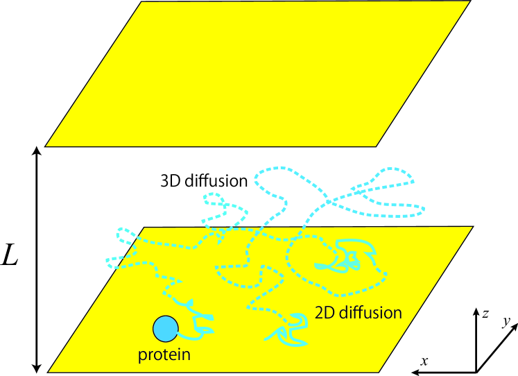
Figure 1: Schematic figure of our model. Diffusivity on the surfaces is different from that in bulk.

III Mean square displacement

Here, we analytically calculate the mean square displacement (MSD) for the cases of exponential and power-law waiting time distributions on the membrane surface. We define the ratio between total residence time on the membrane surfaces and total measurement time as $T_{s}$:

$$T_{s}\equiv\lim_{t\to\infty}\frac{t_{s}^{1}+\cdots+t_{s}^{N_{t}}}{t},$$ (3)

where $t_{s}^{i}$ is the $i$th residence time on the membrane surfaces and $N_{t}$ is the number of visits to the membrane surfaces until time $t$. We note that the ratio is given by the mean residence time on the membrane surfaces $\mu_{s}$ and the mean return time to the membrane surfaces after desorbing from the walls $\mu_{b}$: $T_{s}=\mu_{s}/(\mu_{s}+\mu_{b})$. Furthermore, $\mu_{b}$ is given by $\mu_{b}=3(L-1)\tau_{b}$ because the mean waiting time for the $z$ direction in the bulk is given by $3\tau_{b}$ and the mean first passage time to $z=0$ or $z=L$ starting from $z=1$ or $z=L-1$ is given by $L-1$ times the mean waiting time for an usual random walk in one dimension. As shown in Appendix A, the mean residence time on the membrane surfaces is given by $\mu_{s}=\tau_{z}$ both in the cases of the exponential and power-law waiting-time PDF on the $xy$ plane. More precisely, the PDF of the residence times on the membrane surface is the exactly same form as $\phi(\tau)$.

The MSD for the $x$ direction is given by

$$\langle x_{t}^{2}\rangle=\langle(\Delta x_{t_{s}^{1}}+\Delta x_{t_{b}^{1}}+\cdots+\Delta x_{t_{s}^{N_{t}}}+\Delta x_{t_{b}^{N_{t}}}+\Delta_{t})^{2}\rangle$$ (4)

where $\Delta x_{t_{s}^{i}}$ is the displacement for $x$ direction during the $i$th residence on the membrane surfaces, $\Delta x_{t_{b}^{i}}$ is the displacement for $x$ direction during the $i$th residence in the bulk, and $\Delta_{t}$ is a correction term associated with the last step, where $\langle\Delta_{t}^{2}\rangle$ can be negligibly small when $t$ is sufficiently large, i.e., $\langle\Delta_{t}^{2}\rangle/\langle x_{t}^{2}\rangle\to 0$ as $t\to\infty$. The displacements are given by $\Delta x_{t_{s}^{i}}=x_{t_{i}+t_{s}^{i}}-x_{t_{i}}$ and $\Delta x_{t_{b}^{i}}=x_{t_{i+1}}-x_{t_{i+1}-t_{b}^{i}}$ if the random walker is initially located on the membrane surface, where $t_{i}=\sum_{k=1}^{i-1}(t_{s}^{k}+t_{b}^{k})$. Because the displacements are independent of each other, we have

$$\langle\Delta x_{t_{s}^{i}}\cdot\Delta x_{t_{s}^{j}}\rangle=\langle\Delta x_{t_{b}^{i}}\cdot\Delta x_{t_{b}^{j}}\rangle=0\quad(i\neq j)$$ (5)

and

$$\langle\Delta x_{t_{s}^{i}}\cdot\Delta x_{t_{b}^{j}}\rangle=0.$$ (6)

It follows that the MSD is given by

$$\langle x_{t}^{2}\rangle\sim\sum_{n=1}^{\infty}\Pr(N_{t}=n)\sum_{i=1}^{n}\{\langle\Delta x_{t_{s}^{i}}^{2}\rangle+\langle\Delta x_{t_{b}^{i}}^{2}\rangle\}$$ (7)

for $t\to\infty$.

We note that an equilibrium probability with respect to the $z$ direction exists because there is a confinement for the $z$ direction and the mean residence time on the membrane surface is finite. In particular, the equilibrium probability is given by

$$\rho_{eq}(z)=\left\{\begin{array}[]{ll}\dfrac{\mu_{s}}{2(\mu_{s}+\mu_{b})}&(z=0)\\ \\ \dfrac{\mu_{b}}{(L-1)(\mu_{s}+\mu_{b})}&(0<z<L)\\ \\ \dfrac{\mu_{s}}{2(\mu_{s}+\mu_{b})}&(z=L).\\ \end{array}\right.$$ (8)

III.1 Exponential waiting-time distribution

The diffusion coefficients, defined by $D=\langle{\bm{r}}(t)^{2}\rangle/(2dt)$, in the bulk ($d=3$) and on the membrane surfaces ($d=2$) are given by $1/(6\tau_{b})$ and $1/(4\tau_{s})$, respectively. We use the following notation: $D_{b}=1/(6\tau_{b})$ and $D_{s}=1/(4\tau_{s})$. Because the initial condition for the $z$ position is in equilibrium, we have $\langle N_{t}\rangle=t/(\mu_{s}+\mu_{b})$ Cox (1962). Using $\langle\Delta x_{t_{b}^{i}}^{2}\rangle=2D_{b}t_{b}^{i}$ and $\langle\Delta x_{t_{s}^{i}}^{2}\rangle=2D_{s}t_{s}^{i}$, we obtain the MSD:

$$\langle x_{t}^{2}\rangle\sim 2\left(\frac{D_{s}\mu_{s}}{\mu_{s}+\mu_{b}}+\frac{D_{b}\mu_{b}}{\mu_{s}+\mu_{b}}\right)t$$ (9)

for $t\to\infty$. Because the MSD for the $y$ direction is the same as that for the $x$ direction, the lateral MSD (the MSD on the $xy$ plane) is given by

$$\langle x_{t}^{2}+y_{t}^{2}\rangle\sim 4\left(\frac{D_{s}\mu_{s}}{\mu_{s}+\mu_{b}}+\frac{D_{b}\mu_{b}}{\mu_{s}+\mu_{b}}\right)t$$ (10)

for $t\to\infty$. Therefore, the effective lateral diffusion coefficient, $D_{\rm eff}\equiv\langle x_{t}^{2}+y_{t}^{2}\rangle/(4t)$ as $t\to\infty$, is given by

$$D_{\rm eff}=\frac{D_{s}\mu_{s}+D_{b}\mu_{b}}{\mu_{s}+\mu_{b}}.$$ (11)

The result is consistent with that for diffusion in multilayer media Berezhkovskii and Weiss (2006).

III.2 Power-law waiting time distribution

Equation (7) can be used even when the waiting time distribution is not exponential. To investigate an effect of anomalous diffusion (subdiffusion), i.e., the MSD grows sublinearly with time, on the membrane surface, we consider the following power-law waiting-time distribution on the surfaces, $\psi_{s}(\tau)\sim\frac{\alpha}{\tau_{s}}\left(\frac{\tau}{\tau_{s}}\right)^{-1-\alpha}$ $(\tau\to\infty)$ with $\alpha\leq 1$. In this case, the MSD on the membrane surface shows subdiffusion:

$$\langle x_{t_{s}}^{2}+y_{t_{s}}^{2}\rangle\cong D^{\prime}_{s}t_{s}^{\alpha},$$ (12)

where $D^{\prime}_{s}=1/\Gamma(1-\alpha)\Gamma(1+\alpha)\tau_{s}^{\alpha}$. As in the calculation of the exponential case, we have

$$\langle x_{t}^{2}+y_{t}^{2}\rangle\sim\left(\frac{D^{\prime}_{s}\langle\tau_{s}^{\alpha}\rangle}{\mu_{s}+\mu_{b}}+\frac{2D_{b}\mu_{b}}{\mu_{s}+\mu_{b}}\right)t,$$ (13)

where we have used $\sum_{i+1}^{n}(t_{s}^{i})^{\alpha}/n\to\langle t_{s}^{\alpha}\rangle$. Because the PDF of the residence times on the membrane surface is the same as $\phi(\tau)$, $\langle t_{s}^{\alpha}\rangle$ is given by $\langle t_{s}^{\alpha}\rangle=\tau_{z}^{\alpha}\Gamma(1+\alpha)$. Therefore, the effective lateral diffusion coefficient is given by

$$D_{\rm eff}=\frac{D^{\prime}_{s}\langle t_{s}^{\alpha}\rangle/2+D_{b}\mu_{b}}{\mu_{s}+\mu_{b}}.$$ (14)

Figure 2 shows the MSDs for the exponential and power-law waiting-time PDFs on the surfaces. Theoretical results, Eqs. (10) and (13), are in good agreement with those of simulations. We note that the MSD is always normal because of desorptions. In other words, the MSD does not show a transient subdiffusion even when the MSD on the surface is subdiffusive. This is because the initial condition for $z$ direction is in equilibrium. Otherwise, the MSD asymptotically exhibits normal diffusion (transient subdiffusion).

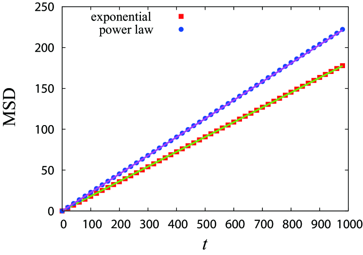
Figure 2: Mean square displacement for different waiting time distributions on the membrane surfaces ($\tau_{b}=1$, $\tau_{z}=100$, and $L=10$). Squares and circles are the results of the numerical simulation in the cases of exponential ($\tau_{s}=20$) and power-law ($\alpha=0.5$ and $\tau_{s}=1$) waiting-time distributions, respectively. In the power-law waiting-time distribution, we use $\psi_{s}(\tau)=\alpha\tau^{-1-\alpha}$ $(\tau\geq 1)$. Solid lines are the theoretical ones.

IV Time-averaged mean square displacement

Here, we consider fluctuations of the lateral TAMSD on $xy$ plane ($d=2$) in the case of the exponential waiting-time distribution. To characterize the fluctuations, we use the RSD, defined by Eq. (2). For an equilibrium process, the ensemble average of TAMSD coincides with the MSD: $\langle\overline{\delta^{2}(\Delta;t)}\rangle=\langle x_{\Delta}^{2}+y_{\Delta}^{2}\rangle$. Therefore, the ensemble average of diffusion coefficients is given by

$$\langle D_{t}\rangle=\frac{D_{s}\mu_{s}+D_{b}\mu_{b}}{\mu_{s}+\mu_{b}},$$ (15)

for all $t>0$.

As shown in Fig. 3, the RSD shows a crossover from a plateau to $t^{-0.5}$ decay. This persistent plateau implies a distributional behavior in diffusivity. In other words, an observed diffusivity before the crossover remains a random variable. When the measurement time $t$ is much smaller than the crossover time $\tau_{c}$, the diffusivity is almost determined by that of an initial state, i.e., bulk or surface. It follows that the probability that diffusion coefficient is $D_{s}$ is almost equal to $T_{s}$ and the probability that diffusion coefficient is $D_{b}$ is almost equal to $1-T_{s}$. Therefore, for $t\ll\tau_{c}$, we have

$$\langle D_{t}^{2}\rangle\cong D_{s}^{2}T_{s}+D_{b}^{2}(1-T_{s})=\frac{D^{2}_{s}\mu_{s}+D^{2}_{b}\mu_{b}}{\mu_{s}+\mu_{b}}.$$ (16)

Thus, the RSD is approximately given by

$$\sigma_{D}(t)\cong\frac{|D_{b}-D_{s}|\sqrt{\mu_{s}\mu_{b}}}{D_{s}\mu_{s}+D_{b}\mu_{b}}.$$ (17)

Recently, theory of the RSD in a diffusion process with a time-dependent and fluctuating diffusivity has been developed Uneyama et al. . Because the lateral diffusion in our model is a two-state diffusion process where the state is randomly fluctuating, we can apply the theory to our model. For $t\gg\tau_{c}$, the theory states that the RSD is given by

$$\sigma_{D}^{2}(t)\cong\frac{2}{t}\int_{0}^{\infty}ds\psi_{1}(s),$$ (18)

where

$$\psi_{1}(t)\equiv\frac{\langle D_{t}D_{0}\rangle-\langle D_{0}\rangle^{2}}{\langle D_{0}\rangle^{2}}.$$ (19)

The correlation function in dichotomous processes is calculated in Appendix. C. It follows that the RSD for $t\gg\tau_{c}$ is obtained as

$$\sigma_{D}(t)\sim\frac{|D_{b}-D_{s}|\mu_{s}\mu_{b}}{D_{s}\mu_{s}+D_{b}\mu_{b}}\sqrt{\left(\frac{\langle\tau_{s}^{2}\rangle_{c}}{\mu_{s}^{2}}+\frac{\langle\tau_{b}^{2}\rangle_{c}}{\mu_{b}^{2}}\right)\frac{1}{(\mu_{s}+\mu_{b})t}},$$ (20)

where $\langle\cdot\rangle_{c}$ is the cumulant. Therefore, the crossover time $\tau_{c}$ from distributional to ergodic behavior is given by

$$\tau_{c}=\frac{\mu_{s}\mu_{b}}{\mu_{s}+\mu_{b}}\left(\frac{\langle\tau_{s}^{2}\rangle_{c}}{\mu_{s}^{2}}+\frac{\langle\tau_{b}^{2}\rangle_{c}}{\mu_{b}^{2}}\right).$$ (21)

V Method revealing an unknown surface diffusivity

In experiments, it is difficult to estimate the exact diffusivity on the surface. This is because a diffusing particle will desorb from the surface. Here, we provide a method revealing the exact diffusivity on the surface, when the bulk diffusion properties are known, i.e., the bulk diffusivity $D_{b}$ and the mean return time $\mu_{b}$. It is important to note that one can obtain the bulk diffusion coefficient $D_{b}$, the mean return time $\mu_{b}$ in bulk, the effective diffusion coefficient $D_{\rm eff}$, $\sigma_{D}(0)$, and the crossover time $\tau_{c}$ by experiments. Using $D_{\rm eff}$ and $\sigma_{D}(0)$, one can know unknown quantities, i.e., the surface diffusion coefficient $D_{s}$ and the mean trapping time on the surface $\mu_{s}$. In fact, these quantities are explicitly obtained as

$$D_{s}=\frac{D_{\rm eff}(D_{\rm eff}\sigma_{D}(0)^{2}+D_{\rm eff}-D_{b})}{D_{\rm eff}-D_{b}},$$ (22)

and

$$\mu_{s}=\frac{\mu_{b}(D_{\rm eff}-D_{b})}{D_{\rm eff}^{2}\sigma_{D}(0)^{2}}.$$ (23)

In case that $\mu_{b}$ is unknown, we can obtain the ratio $\mu_{s}/\mu_{b}$ from Eq. (23). Moreover, using $\tau_{c}$, one can know the cumulant $\langle\tau_{s}^{2}\rangle_{c}$, i.e., the second moment of the trapping time $\tau_{s}$. We note that this crossover time is important to know a characteristic time in the diffusivity. In fact, this crossover time is related to the longest relaxation time in entangled polymers Uneyama et al. (2012, ). In general, it is difficult to determine whether a particle is on the surface or not in experiments. Therefore, this is a good method to estimate the surface properties because this method does not require a determination of whether a particle is on the surface or not.

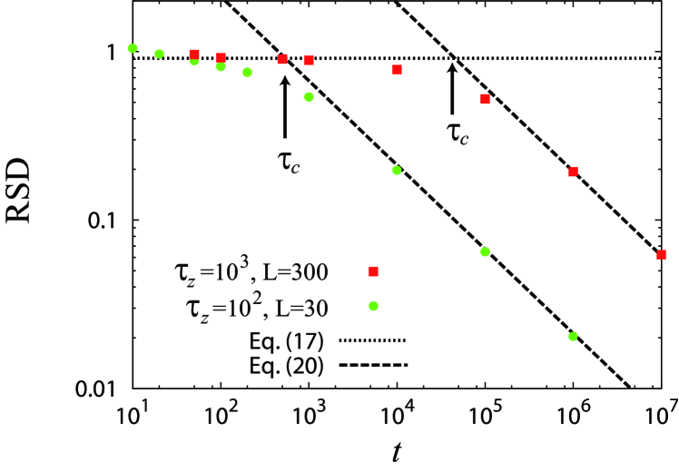
Figure 3: Relative standard deviation of the TAMSDs ($\tau_{b}=1$, $\tau_{s}=20$, and $L=10$). In numerical simulations, we replace $D_{t}$ as $\overline{\delta^{2}(\Delta;t)}$ with $\Delta=20$ because the TAMSDs show normal diffusion, which is confirmed numerically (not shown). The dashed lines are the theoretical ones described by Eq. (17) and (20), where the second moment $\langle\tau_{s}^{2}\rangle$ is obtained numerically.

VI Conclusion

We have shown that the ensemble-averaged MSDs show normal diffusion even when the diffusion on the surface is not normal (subdiffusion). Moreover, we find that fluctuations of TAMSDs remain random if the measurement time is smaller than a characteristic relaxation time even when the process is in equilibrium. For large measurement times, the fluctuations decay as $t^{-0.5}$, which is a usual ergodic relaxation. In other words, we find a transition from a non-ergodic (distributional) behavior to an ergodic behavior. Although a similar phenomenon was found in CTRW where the waiting-time distribution has a power law with an exponential cutoff Miyaguchi and Akimoto (2011b), the transition in our model results from a two-state randomly fluctuating diffusivity, which is a completely different origin from CTRW. Such a two-state diffusion process is an optimal target search process because a searching molecule can bind to the target with the aid of the slow diffusivity near the target (surface). We suggest that the transition from non-ergodic to ergodic behavior will be universal in optimal target search processes.

TA thanks T. Uneyama and T. Miyaguchi for discussion about Eq. (18). This work was supported in part by Grant for Basic Science Research Projects from The Sumitomo Foundation.

Appendix A Derivation of the PDF of residence times on the membrane surface

In our model, a random walker desorbs from the membrane surface if the waiting time for the $z$ direction is smaller than that for the $xy$ plane. Let $X_{i}$ and $Y_{i}$ be random variables with distributions $\psi_{s}(x)$ and $\phi(y)$, respectively. Then, the residence time can be represented by

$$T=Z_{1}+Z_{2}+\cdots+Z_{n-1}+Z_{n},$$ (24)

where $n=\min\{k\leq 1;Y_{k}<X_{k}\}$ and $Z_{k}$ be the minimum of $X_{k}$ and $Y_{k}$: $Z_{k}\equiv\min(X_{k},Y_{k})$. Using Eq. (24), we can derive the PDF of the residence times on the membrane surface. The PDFs of random variables $Z_{k}$ with $X_{k}<Y_{k}$ and $Y_{k}<X_{k}$ are given by

$$\psi_{Z_{X}}(\tau)=\psi_{s}(\tau)\int_{\tau}^{\infty}\phi(x)dx$$ (25)

and

$$\psi_{Z_{Y}}(\tau)=\phi(\tau)\int_{\tau}^{\infty}\psi_{s}(x)dx,$$ (26)

respectively. The Laplace transform of the PDF $P(T)$ is written as

$$P^{*}(s)=\sum_{n=1}^{\infty}\{\psi_{Z_{X}}^{*}(s)\}^{n-1}\psi_{Z_{Y}}^{*}(s)=\frac{\psi_{Z_{Y}}^{*}(s)}{1-\psi_{Z_{X}}^{*}(s)},$$ (27)

where $\psi_{Z_{Y}}^{*}(s)$ and $\psi_{Z_{Y}}^{*}(s)$ are the Laplace transforms of $\psi_{Z_{X}}(\tau)$ and $\psi_{Z_{Y}}(\tau)$, respectively. Because $\phi(\tau)=\tau_{z}^{-1}\exp(-\tau/\tau_{z})$, the Laplace transforms of $\psi_{Z_{X}}(\tau)$ and $\psi_{Z_{Y}}(\tau)$ are given by

$$\psi_{Z_{X}}^{*}(s)=\psi_{s}(s+\tau_{z}^{-1})$$ (28)

and

$$\psi_{Z_{Y}}^{*}(s)=\frac{1}{\tau_{z}}\frac{1-\psi_{s}(s+\tau_{z}^{-1})}{s+\tau_{z}^{-1}},$$ (29)

respectively. Therefore, we have

$$P^{*}(s)=\frac{1}{1+s\tau_{z}},$$ (30)

which means $P(T)=\phi(T)$.

Appendix B Lateral subdiffusion in CTRW

It is known that the MSD in CTRW with the waiting time PDF $\psi_{s}(\tau)\sim\frac{\alpha}{\tau_{s}}\left(\frac{\tau}{\tau_{s}}\right)^{\alpha}$ ($\tau\to\infty$) is given by

$$\langle x_{t}^{2}\rangle\sim\frac{1}{\Gamma(1-\alpha)\Gamma(1+\alpha)}\left(\frac{t}{\tau_{s}}\right)^{\alpha}$$ (31)

for $t\to\infty$ Metzler and Klafter (2000). In our model, if a random walker does not desorb from the surface, a waiting time is assigned and it will jump to the $x$ or $y$ direction with equal probability. Because the waiting time PDF for the $x$ direction in our model can be written as its convolution, the Laplace transform of the PDF is given by

$$\psi^{*}_{x}(s)=\sum_{n=1}^{\infty}\{\psi^{*}_{s}(s)\}^{n}\frac{1}{2^{n}}=\frac{\psi^{*}_{s}(s)/2}{1-\psi^{*}_{s}(s)/2}.$$ (32)

Using the Laplace transform $\psi_{s}^{*}(s)$, we obtain

$$\psi_{x}^{*}(s)=1-2\tau_{s}^{\alpha}s^{\alpha}+o(s^{\alpha}).$$ (33)

The waiting time PDF for $x$ direction is given by

$$\psi_{x}(\tau)\sim\frac{\alpha}{2^{\frac{1}{\alpha}}\tau_{s}}\left(\frac{\tau}{2^{\frac{1}{\alpha}}\tau_{s}}\right)^{-1-\alpha}$$ (34)

for $\tau\to\infty$. It follows that the lateral MSD is given by

$$\langle x_{t}^{2}+y_{t}^{2}\rangle\sim\frac{1}{\Gamma(1-\alpha)\Gamma(1+\alpha)}\left(\frac{t}{\tau_{s}}\right)^{\alpha}{\color[rgb]{0,0,1}.}$$ (35)

Appendix C Correlation function in dichotomous processes

We calculate the correlation function, defined by $C(t)\equiv\langle D_{t}D_{0}\rangle-\langle D_{0}\rangle^{2}$, in two-state process (dichotomous process). The correlation function is represented by

$$C(t) = D_{b}^{2}P_{b}W_{bb}(t)+D_{b}D_{s}P_{s}W_{bs}(t)$$ (36)

$$+D_{s}D_{b}P_{b}W_{sb}+D_{s}^{2}P_{s}W_{ss}(t)-\langle D_{0}\rangle^{2},$$

where $P_{b}$ and $P_{s}$ are the probabilities of finding a particle initially in the bulk and on the surface, respectively. $W_{bb}(t)=\Pr\{D_{t}=D_{b}|D_{0}=D_{b}\}$, $W_{bs}(t)=\Pr\{D_{t}=D_{s}|D_{0}=D_{b}\}$, $W_{sb}(t)=\Pr\{D_{t}=D_{b}|D_{0}=D_{s}\}$, and $W_{ss}(t)=\Pr\{D_{t}=D_{s}|D_{0}=D_{s}\}$ are conditional probabilities, and $\langle D_{0}\rangle$ is given by

$$\langle D_{0}\rangle=\frac{D_{b}\mu_{b}+D_{s}\mu_{s}}{\mu_{b}+\mu_{s}}.$$ (37)

The conditional probability can be obtained as

$$W_{bb}(t) = \sum_{n=0}^{\infty}\Pr(N_{t}=2n)$$ (39)

$$= \sum_{n=1}^{\infty}\{\Pr(S_{2n}<t)-\Pr(S_{2n+1}<t)\}$$

$$+\Pr(N_{t}=0),$$

where $S_{n}$ is a sum of waiting times, i.e., $S_{2n}={\tau_{s}^{1}}+{\tau_{b}^{1}}+\cdots+{\tau_{s}^{n}}+{\tau_{b}^{n}}$. Therefore, the Laplace transform is given by

$$\hat{W}_{bb}(s) = \frac{1}{s}\sum_{n=1}^{\infty}\hat{f}_{E,b}(s)\{\hat{\psi}_{s}(s)\hat{\psi}_{b}(s)\}^{n-1}\hat{\psi}_{s}(s)-\frac{1}{s}\sum_{n=1}^{\infty}\hat{f}_{E,b}(s)\{\hat{\psi}_{s}(s)\hat{\psi}_{b}(s)\}^{n}+\frac{1-\hat{f}_{E,b}(s)}{s}$$ (40)

$$= \frac{1}{s}-\frac{\hat{f}_{E,b}(s)}{s}\frac{1-\hat{\psi}_{s}(s)}{1-\hat{\psi}_{b}(s)\hat{\psi}_{s}(s)},$$ (41)

where $\hat{f}_{E,b}(s)$ is the Laplace transform of the PDF of the forward recurrence time $\hat{f}_{E,b}(\tau)$ when the random walker is in bulk, which is given by $\hat{f}_{E,b}(s)=[1-\hat{\psi}_{b}(s)]/(\mu_{b}s)$ Cox (1962); Godrèche and Luck (2001). In the same way as in Eq. (41), we have

$$\hat{W}_{ss}(s)=\frac{1}{s}-\frac{\hat{f}_{E,s}(s)}{s}\frac{1-\hat{\psi}_{b}(s)}{1-\hat{\psi}_{b}(s)\hat{\psi}_{s}(s)},$$ (42)

$$\hat{W}_{bs}(s)=\frac{1}{s}-\frac{\hat{f}_{E,b}(s)}{s}\frac{1-\hat{\psi}_{s}(s)}{1-\hat{\psi}_{b}(s)\hat{\psi}_{s}(s)},$$ (43)

and

$$\hat{W}_{sb}(s)=\frac{1}{s}-\frac{\hat{f}_{E,s}(s)}{s}\frac{1-\hat{\psi}_{b}(s)}{1-\hat{\psi}_{b}(s)\hat{\psi}_{s}(s)},$$ (44)

where $\hat{f}_{E,s}(s)$ is the Laplace transform of the PDF of the forward recurrence time $\hat{f}_{E,s}(\tau)$ when the random walker is on the surface, which is given by $\hat{f}_{E,s}(s)=[1-\hat{\psi}_{s}(s)]/(\mu_{s}s)$ Cox (1962); Godrèche and Luck (2001). It follows that the Laplace transform of $C(t)$ is given by

$$\hat{C}(s) = \left(\frac{D_{b}-D_{s}}{\mu_{b}+\mu_{s}}\right)^{2}\frac{\mu_{b}\mu_{s}}{s}$$ (45)

$$-\frac{(D_{b}-D_{s})^{2}}{\mu_{b}+\mu_{s}}\frac{\{1-\hat{\psi}_{b}(s)\}\{1-\hat{\psi}_{s}(s)\}}{\{1-\hat{\psi}_{b}(s)\hat{\psi}_{s}(s)\}s^{2}}.$$

Because we assume that all moments of the waiting times are finite, the Laplace transform becomes

$$\hat{C}(s)=\frac{(D_{b}-D_{s})^{2}(\mu_{b}\mu_{s})^{2}}{2(\mu_{b}+\mu_{s})^{3}}\left(\frac{\langle\tau_{b}^{2}\rangle_{c}}{\mu_{b}^{2}}+\frac{\langle\tau_{s}^{2}\rangle_{c}}{\mu_{s}^{2}}\right)+O(s).$$ (46)

in the small $s\ll 1$. The integration in Eq. (18) can be performed using $\int_{0}^{\infty}ds\psi_{1}(s)=\hat{\psi}_{1}(0)=\frac{\hat{C}(0)}{\langle D_{0}\rangle^{2}}$. Therefore, we obtain Eq. (20).

References

- Bénichou et al. (2011) O. Bénichou, C. Loverdo, M. Moreau, and R. Voituriez, Rev. Mod. Phys. 83, 81 (2011).
- Coppey et al. (2004) M. Coppey, O. Bénichou, R. Voituriez, and M. Moreau, Biophys. J. 87, 1640 (2004).
- Mirny et al. (2009) L. Mirny, M. Slutsky, Z. Wunderlich, A. Tafvizi, J. Leith, and A. Kosmrlj, J. Phys. A 42, 434013 (2009).
- Grossman et al. (2011) M. Grossman, B. Born, M. Heyden, D. Tworowski, G. B. Fields, I. Sagi, and M. Havenith, Nat. Struct. Mol. Biol. 18, 1102 (2011).
- Yamamoto et al. (2013) E. Yamamoto, T. Akimoto, Y. Hirano, M. Yasui, and K. Yasuoka, Phys. Rev. E 87, 052715 (2013).
- Yamamoto et al. (2014) E. Yamamoto, T. Akimoto, M. Yasui, and K. Yasuoka, Sci. Rep. 4, 4720 (2014).
- Ball (2011) P. Ball, Nature 478, 467 (2011).
- Fuliński (2011) A. Fuliński, Phys. Rev. E 83, 061140 (2011).
- Cherstvy et al. (2013) A. G. Cherstvy, A. V. Chechkin, and R. Metzler, New J. Phys. 15, 083039 (2013).
- Cherstvy and Metzler (2013) A. G. Cherstvy and R. Metzler, Phys. Chem. Chem. Phys. 15, 20220 (2013).
- Jeon et al. (2014) J.-H. Jeon, A. Checkin, and R. Metzler, Phys. Chem. Chem. Phys. 16, 15811 (2014).
- (12) T. Uneyama, T. Miyaguchi, and T. Akimoto, ArXiv:1411:5165.
- Golding and Cox (2006) I. Golding and E. C. Cox, Phys. Rev. Lett. 96, 098102 (2006).
- Weigel et al. (2011) A. Weigel, B. Simon, M. Tamkun, and D. Krapf, Proc. Natl. Acad. Sci. USA 108, 6438 (2011).
- Jeon et al. (2011) J.-H. Jeon, V. Tejedor, S. Burov, E. Barkai, C. Selhuber-Unkel, K. Berg-Sørensen, L. Oddershede, and R. Metzler, Phys. Rev. Lett. 106, 048103 (2011).
- Tabei et al. (2013) S. A. Tabei, S. Burov, H. Y. Kim, A. Kuznetsov, T. Huynh, J. Jureller, L. H. Philipson, A. R. Dinner, and N. F. Scherer, Proc. Natl. Acad. Sci. USA 110, 4911 (2013).
- Lubelski et al. (2008) A. Lubelski, I. M. Sokolov, and J. Klafter, Phys. Rev. Lett. 100, 250602 (2008).
- He et al. (2008) Y. He, S. Burov, R. Metzler, and E. Barkai, Phys. Rev. Lett. 101, 058101 (2008).
- Miyaguchi and Akimoto (2013) T. Miyaguchi and T. Akimoto, Phys. Rev. E 87, 032130 (2013).
- Metzler et al. (2014) R. Metzler, J.-H. Jeon, A. G. Cherstvy, and E. Barkai, Phys. Chem. Chem. Phys. 16, 24128 (2014).
- Miyaguchi and Akimoto (2011a) T. Miyaguchi and T. Akimoto, Phys. Rev. E 83, 031926 (2011a).
- Miyaguchi and Akimoto (2011b) T. Miyaguchi and T. Akimoto, Phys. Rev. E 83, 062101 (2011b).
- Knight and Falke (2009) J. D. Knight and J. J. Falke, Biophys. J. 96, 566 (2009).
- Knight et al. (2010) J. D. Knight, M. G. Lerner, J. G. Marcano-Velázquez, R. W. Pastor, and J. J. Falke, Biophys. J. 99, 2879 (2010).
- Rozovsky et al. (2012) S. Rozovsky, M. B. Forstner, H. Sondermann, and J. T. Groves, J. Phys. Chem. B 116, 5122 (2012).
- Skaug et al. (2014) M. J. Skaug, A. M. Lacasta, L. Ramirez-Piscina, J. M. Sancho, K. Lindenberg, and D. K. Schwartz, Soft Matter 10, 753 (2014).
- Bénichou et al. (2010) O. Bénichou, D. Grebenkov, P. Levitz, C. Loverdo, and R. Voituriez, Phys. Rev. Lett. 105, 150606 (2010).
- Bénichou et al. (2011) O. Bénichou, D. Grebenkov, P. Levitz, C. Loverdo, and R. Voituriez, J. Stat. Phys. 142, 657 (2011).
- Rupprecht et al. (2012a) J.-F. Rupprecht, O. Bénichou, D. Grebenkov, and R. Voituriez, J. Stat. Phys. 147, 891 (2012a).
- Rupprecht et al. (2012b) J.-F. Rupprecht, O. Bénichou, D. S. Grebenkov, and R. Voituriez, Phys. Rev. E 86, 041135 (2012b).
- Cox (1962) D. R. Cox, Renewal theory (Methuen, London, 1962).
- Berezhkovskii and Weiss (2006) A. M. Berezhkovskii and G. H. Weiss, J. Chem. Phys. 124, 154710 (2006).
- Uneyama et al. (2012) T. Uneyama, T. Akimoto, and T. Miyaguchi, J. Chem. Phys. 137, 114903 (2012).
- Metzler and Klafter (2000) R. Metzler and J. Klafter, Phys. Rep. 339, 1 (2000).
- Godrèche and Luck (2001) C. Godrèche and J. M. Luck, J. Stat. Phys. 104, 489 (2001).