Geometry, robustness, and emerging unitarity in dissipation-projected dynamics

Abstract

Quantum information can be encoded in the set of steady-states (SSS) of a driven-dissipative system. Non steady-states are separated by a large dissipative gap that adiabatically decouples them way while the dynamics inside the SSS is governed by an effective, dissipation-projected, Hamiltonian. The latter results from a highly non-trivial interplay between a weak driving with the fast relaxation process that continuously projects the system back to the SSS. This amounts to a novel type of environment-induced quantum Zeno effect. We prove that the dissipation-projected dynamics is of geometric nature and that it is robust against different types of hamiltonian and dissipative perturbations. Remarkably, in some cases an effective unitary dynamics can emerge out of purely dissipative interactions.

I Introduction

Since the earliest days of quantum information processing (QIP) weak coupling to the environmental degrees of freedom has been regarded as one of the essential prerequisites. In fact decoherence and dissipation generally spoil the unitary character of the quantum dynamics and induce errors into the computational process. In order to overcome such an obstacle a variety of techniques have been devised including quantum error correction QEC , decoherence-free subspaces (DFSs) DFS ; DFS1 ; DFS-exp , noiseless subsystems (NS) NS ; stab ; NS-top ; NS-exp and geometric/holonomic quantum computation Jones ; HQC ; HQC-science .

However, it has been recently realized that dissipation and decoherence may even play a positive role to the aim of coherent quantum manipulations. Indeed, it has been shown that, properly engineered, dissipative dynamics can in principle be used to enact QIP primitives such as quantum state preparation Kraus-prep ; kastoryano2011dissipative , quantum simulation barreiro2011open and computation verstraete2009quantum . Exotic physical properties such as topological order dissi-top and non-abelian synthetic gauge fields gauge can also be achieved by engineered dissipation.

In a nutshell the idea is that one can design driven-dissipative systems such that their steady-states enjoy some computationally desirable property. For example in Ref. kastoryano2011dissipative the unique steady-state is maximally entangled, while in Ref. verstraete2009quantum the steady states encode for an arbitrary quantum computation! Moreover, the irreversible and attractive nature of dissipative dynamics endows these techniques with a degree of robustness against imperfections in preparation and control. All this leads to a dramatic paradigm shift in QIP: noise and dissipation should not be viewed as detrimental but may in fact be considered as a resource.

In this paper we will build upon our recent discovery on how to enact coherent dynamics over the set of steady states (SSS) of a strongly dissipative system zanardi-dissipation-2014 . Quantum information is encoded in sectors of the SSS while non steady-states are separated by the large dissipative gap that adiabatically decouples them away. A weak Hamiltonian control gives rise to an effective dynamics inside the SSS that is ruled by a dissipation-projected Hamiltonian. The latter results from a highly non-trivial interplay between the control and the fast relaxation process that continuously projects the system back onto the SSS. This amounts to a novel type of environment-induced quantum Zeno effect zeno-subspaces ; dan-zeno .

In this paper we will show that the dissipation-projected dynamics is geometric in nature. This means that this approach can be regarded as a dissipative extension of the fault-tolerant techniques of geometric and holonomic quantum computation Jones ; HQC ; HQC-science . We will also prove that the dissipation-projected Hamiltonians are protected against several types of perturbations (unitary and dissipative) and may allow for robust QIP. Finally we will show how an effective unitary evolution may emerge out of suitable dissipative perturbations of a purely dissipative dynamics. This “emerging unitarity" phenomenon is perhaps the single most surprising one of our results.

II The dissipation-projection theorem

We will consider quantum open systems whose dynamics is described by the equation

$$\frac{d\rho(t)}{dt}={\cal L}\,\rho(t).$$ (1)

The superoperator ${\cal L}$ will be referred as to the Liouvillian An open quantum system generically admits a unique steady-state $\rho_{\infty}$ that is approached by the time-evolving density matrix $\rho(t)$ as the time goes to infinity. Asymptotically the information-theoretic distance $D(\rho(t),\,\rho_{\infty}):=\frac{1}{2}\|\rho(t)-\rho_{\infty}\|_{1}$ decays exponentially with time where the time-scale $\tau_{R}$ is referred to as the relaxation time. For $t\gg\tau_{R}$ the time-evolved state becomes indistinguishable from the steady state. According to Eq. (1) the steady state satisfies ${\cal L}(\rho_{\infty})=0$ i.e. it lies lies in the kernel of the Liouvillian. Uniqueness of the steady-state translates into a one-dimensional kernel. In this paper we will focus on the case in which the Liouvillian can be decomposed as ${\cal L}={\cal L}_{0}+{\cal L}_{1}$ in such a way that

• i) The relaxation time of ${\cal L}_{0}$ is the shortest time-scale of the problem. Equivalently, the dissipative gap of ${\cal L}_{0}$, $\tau_{R}^{-1}$, is the largest energy scale.

• ii) The kernel of ${\cal L}_{0}$ is high-dimensional and attractive (the non-zero eigenvalues of ${\cal L}_{0}$ have a negative real part)

We will denote by ${\cal P}_{0}$ (${\cal Q}_{0}=1-{\cal P}_{0}$) the projection onto the kernel of ${\cal L}_{0}$ (its complementary). The steady-state set (SSS) is given by those states $\rho$ such that ${\cal P}_{0}(\rho)=\rho.$ The critical assumption is that the SSS is high-dimensional. A prototypical instance of this non-generic situation is the following:

Example 0.- Suppose a system $S$ is joined to a system $B$ and that the dissipation acts only on the latter. Let $\rho_{B}$ denote the (generically) unique steady-state of $B$ and by $\rho$ any state of $S$. It is then obvious that any bi-partite state of the form $\rho\otimes\rho_{B}$ is a steady-state of the full dynamical system when the $S$ and $B$ are decoupled. Clearly, any transformation over $S$ is a symmetry of the dynamics. For the sake of concreteness one may think of a two-level atom $S$ strongly coupled to a leaky cavity mode $B$. To a good approximation dissipation acts directly just on $B.$ Formally, the Hilbert space is ${\cal H}={\cal H}_{S}\otimes{\cal H}_{B}$ and ${\cal L}_{0}={\mathbf{1}}_{S}\otimes{\cal L}_{B}$ where the Liouvillian ${\cal L}_{B}$ admits a unique steady-state $\rho_{B}$. In this case ${\cal P}_{0}(X)={\mathrm{Tr}}_{B}(X)\otimes\rho_{B},$ the kernel of ${\cal L}_{0}$ has dimension $({\mathrm{dim}}\,{\cal H}_{S})^{2},$ and the SSS can be identified with the state-space of $S.$ This apparently trivial example will be later considerably generalized resorting to the theory of NSs NS .

The fundamental technical result we would like to build upon is the following fact proved in zanardi-dissipation-2014 (see also Sec. A): Projection Theorem.- Suppose ${\cal L}={\cal L}_{0}+{\cal L}_{1}$ with $\|{\cal L}_{1}\|=O(1/T)$ then

$$\sup_{t\in[0,T]}\|({\cal E}_{t}-e^{t{{\cal L}}_{{\textrm{{eff}}}}}){\cal P}_{0}\|=O(1/{T})$$ (2)

where ${{\cal L}}_{{\textrm{eff}}}:={\cal P}_{0}\,{{\cal L}}\,{\cal P}_{0}={\cal P}_{0}\,{{\cal L}_{1}}\,{\cal P}_{0}$ and ${\cal E}_{t}=e^{t{\cal L}}.$

In words: if the system is prepared at time $t=0$ inside the SSS then, in the large $T$ limit, the time-evolution leaves the SSS invariant and it is governed by the effective generator ${\cal L}_{{\textrm{eff}}}$.

In several of the applications we will discuss below the perturbation will be of Hamiltonian type i.e., ${\cal L}_{1}=-i[K,\bullet],\,(K=K^{\dagger});$ in that case it will be denoted by ${\cal K}.$ The key point is that ${\cal K}_{{\textrm{eff}}}={\cal P}_{0}\,{{\cal K}}\,{\cal P}_{0}$ turns out to be an Hamiltonian; it will be referred to as the dissipation-projected Hamiltonian. Physically, this means that strong dissipation, while dressing the Hamiltonian by a continuous projection onto the SSS, does not alter its unitary character. Non steady-states are adiabatically decoupled away. The SSS and unitarity are protected by the large dissipative gap of ${\cal L}_{0}.$

For example, in the Example 0 discussed above, where the Liouvillian ${\cal L}_{B}$ has a unique steady-state $\rho_{B}$, one finds ${\cal K}_{{\textrm{eff}}}=-i[K_{{\textrm{eff}}},\,\bullet]$ where $K_{{\textrm{eff}}}={\mathrm{Tr}}_{B}(K\rho_{B})\otimes{\mathbf{1}}_{B}$. We see that in fact ${\cal K}_{{\textrm{eff}}}$ is Hamiltonian.

In Sec. A we prove Eq. (2) and we give a rigorous estimate for the coefficient in its RHS. It turns out [see Eq. (40)] that the numerical factor is $c\tau_{R}$ where $\tau_{R}$ is the relaxation time of the unperturbed dynamics and $c$ is a $O(1)$ constant. This fact is important as it implies that the error can be made small, either by making $T$ larger (which also makes the waiting time $O(T)$ longer) or by making dissipation faster (i.e. $\tau_{R}$ smaller). Indeed, measuring times in unit of $\tau_{R}$ one realizes that the expansion parameter in Eq. (2) is really $\tau_{R}/T$. In other terms the “long $T$ limit” just means that the Hamiltonian norm has to be much smaller than the dissipative gap [$=O(\tau_{R}^{-1})]$. The latter represents the physical quantity that in real applications has to be engineered in order to make it as large as possible. Equivalently, one wants to make the relaxation time $\tau_{R}$ as short as possible. We have to operate in the deep dissipative regime.

III Dissipative Holonomies

Let us now discuss the intimate relation between our basic result (2) and geometric and holonomic quantum computation Jones ; HQC . We will show that the effective evolution (2) is in fact geometric and is given by a super-operator holonomy.

The possibility of merging dissipation dynamics and holonomic quantum computation HQC ; HQC1 ; HQC-science by reservoir engineering was first suggested in Refs. angelo ; ogy . More specifically, in angelo a time-dependent Lindbladian dynamics admitting a DFS was considered, and it was shown that under a suitable adiabatic condition, a state initially in a DFS remains inside the subspace and, hence, is rigidly transported around the Hilbert space together with the DFS. The evolution is, in fact, coherent, although entirely produced by an incoherent phenomenon. Moreover, when the DFS eventually returns to its initial configuration, the net effect is a holonomic transformation on the states in the subspace. Counterintuitively, the effect of the dissipation on the (time-dependent) DFS can be made smaller by making the dissipation rate larger. The authors qualitatively explain this phenomenon in terms of some sort of environment-induced quantum Zeno effect where the action of a strong environment can be regarded as a measuring apparatus continuously monitoring the slowly moving DFS.

In order to establish a connection between these findings and the results we have discussed so far it suffices to move to a rotated reference frame by defining $\tilde{\rho}(t):={\cal U}_{t}^{\dagger}\rho(t)$ where ${\cal U}_{t}(X):=e^{t{\cal K}}(X)=e^{-itK}Xe^{itK}.$ In this rotated frame $\tilde{\rho}(t)$ evolves in a time-dependent bath

$$\frac{d\tilde{\rho}(t)}{dt}={\cal L}_{t}\,\tilde{\rho}(t),\qquad{\cal L}_{t}:={\cal U}_{t}^{\dagger}{\cal L}_{0}{\cal U}_{t}$$ (3)

In the rotated frame the dynamical semi-group is given by $\tilde{{\cal E}}_{t}={\cal U}_{t}^{\dagger}{\cal E}_{t}$ and a state $\tilde{\rho}_{t}$ is an instantaneous steady-state of ${\cal L}_{t}$ iff $\tilde{\rho}_{t}={\cal U}_{t}^{\dagger}\rho_{0}$ where $\rho_{0}$ is a steady-state of ${\cal L}_{0}.$ It follows that the projector onto the kernel of ${\cal L}_{t}$ is given by ${\cal P}_{t}={\cal U}_{t}^{\dagger}{\cal P}_{0}{\cal U}_{t}=e^{-t{\cal K}}{\cal P}_{0}e^{t{\cal K}}.$ Moreover, in the rotated-frame the dissipation-projected dynamics is geometric. Proposition 1.– a) The Projection Theorem (2) can be reformulated in the form

$$\|\tilde{{\cal E}}_{t}\,{\cal P}_{0}-{\mathbf{T}}\exp(\int_{0}^{t}d\tau\,[\dot{{\cal P}}_{\tau},\,{\cal P}_{\tau}])\,{\cal P}_{0}\|=O(1/T)$$ (4)

where ${\mathbf{T}}$ denotes the chronological ordering symbol.

b) The ${\mathbf{T}}$-ordered geometric superoperator in (4) can be rewritten as

$$X(t)=\lim_{N\to\infty}{\mathbf{T}}\prod_{j=1}^{N}{\cal P}_{t_{j}}=e^{-t{\cal K}}\lim_{N\to\infty}\left(e^{\frac{t}{N}{\cal K}}{\cal P}_{0}\right)^{N}$$ (5)

where $t_{j}=j{t}/{N},\,j=0,\ldots,N$. Namely the evolution corresponds to an infinite, time-ordered, succession of projections onto the instantaneous SSS. Equivalently, to a succession of ${\cal P}_{0}$ interleaved with infinitesimal unitaries evolutions $e^{\frac{1}{N}{\cal K}}.$

Proof.– a) From unitarity of ${\cal U}_{t}=e^{t{\cal K}}$ and Eq.  (2) one has

$$\|{\cal E}_{t}{\cal P}_{0}-e^{t{\cal P}_{0}{\cal K}{\cal P}_{0}}{\cal P}_{0}\|=\|\tilde{{\cal E}}_{t}{\cal P}_{0}-X(t)\|=O(1/T)$$ (6)

where $X(t):=e^{-t{\cal K}}e^{t{\cal P}_{0}{\cal K}{\cal P}_{0}}{\cal P}_{0}.$ By differentiation

$$\dot{X}(t)=-{\cal K}e^{-t{\cal K}}e^{t{\cal P}_{0}{\cal K}{\cal P}_{0}}{\cal P}_{0}+e^{-t{\cal K}}{\cal P}_{0}{\cal K}{\cal P}_{0}e^{t{\cal P}_{0}{\cal K}{\cal P}_{0}}{\cal P}_{0}=\\ -{\cal K}{\cal P}_{t}X(t)+{\cal P}_{t}{\cal K}X(t)=[-{\cal K},\,{\cal P}_{t}]X(t)=\dot{{\cal P}}_{t}\,X(t)$$ (7)

Notice also that ${\cal P}_{t}X(t)=X(t)$ and ${\cal P}_{t}\dot{{\cal P}}_{t}{\cal P}_{t}=0,$ whence $\dot{X}(t)=\dot{{\cal P}}_{t}\,X(t)=\dot{{\cal P}}_{t}{\cal P}_{t}\,X(t)=(\dot{{\cal P}}_{t}{\cal P}_{t}-{\cal P}_{t}\dot{{\cal P}}_{t})\,{\cal P}_{t}X(t),$ namely

$$\frac{dX(t)}{dt}=[\dot{{\cal P}}_{t},\,{\cal P}_{t}]\,X(t)\Rightarrow X(t)={\mathbf{T}}\,e^{\int_{0}^{t}d\tau\,[\dot{{\cal P}}_{\tau},\,{\cal P}_{\tau}]}X(0).$$ (8)

Eq. (4) is now obtained by using (6) and $X(0)={\cal P}_{0}.$

b) Proceeding formally, if $\tilde{X}(t)=\prod_{\tau\in[0,\,t]}{\cal P}_{\tau}$ then

$$\tilde{X}(t+dt)-\tilde{X}(t)={\cal P}_{t+dt}\tilde{X}(t)-\tilde{X}(t)=\\ ({\cal P}_{t+dt}-{\cal P}_{t})\tilde{X}(t)=\dot{{\cal P}}_{t}\tilde{X}(t)dt+O(dt^{2}).$$ (9)

Whence $\dot{\tilde{X}}(t)=\dot{{\cal P}}_{t}\tilde{X}(t)$. Since $X(t)$ and $\tilde{X}(t)$ fulfill the same ODE and the same initial condition $X(0)=\tilde{X}(0)={\cal P}_{0}$ they have to be the same function. This proves the first equality in (5) while the second can be verified by direct inspection using the definition of the ${\cal P}_{t}$’s. $\hfill\Box$ The integral in (4) is clearly invariant under time reparametrizations $\tau\to\tau^{\prime}=\tau^{\prime}(\tau)$ and it is therefore of geometric nature i.e., it depends only on the path $t\to{\cal P}_{t}$ in the space of (super) projections. We also see that the super-operator holonomy is the line integral of the “tautological” connection ${\cal A}=[\dot{{\cal P}}(\tau),\,{\cal P}(\tau)]$ Nak .

If one replaces in Eq. (5) the projection ${\cal P}_{0}$ with a more-general CP map e.g., generalized measurement, basically all the Quantum-Zeno like QIP protocols recently discussed in the literature are recovered ogy ; HQC-zeno ; cave ; kwek-zeno . In all these works the geometric and holonomic nature of the resulting dynamics have been discussed on the basis of the particular case at hand, and a general comprehensive theoretical understanding seems to be lacking. The dissipation-projection theorem (2) seems able to provide such an underlying conceptual framework.

IV SSS and Interaction Algebras

In this section we would like to discuss an important class of dissipative systems whose SSS can be fully characterized on general algebraic grounds and at the same time describes physically relevant cases.

Let us consider the most general dissipative generator ${\cal L}_{0}$ of a Markovian quantum dynamical semi-group ${\cal E}_{t}:=e^{t\,{\cal L}_{0}}$. Thanks to the Lindblad theorem Lindblad-paper the Liouvillian can be written as

$${\cal L}_{0}(\rho)=\sum_{\alpha}(L_{\alpha}\rho L_{\alpha}^{\dagger}-\frac{1}{2}\{L_{\alpha}^{\dagger}L_{\alpha},\,\rho\})$$ (10)

The $L_{\alpha}$’s are the co-called Lindblad operators. Let us now define two operator algebras associated with (10)

$${\cal A}:={\mathrm{Alg}}[\{L_{\alpha},\,L_{\alpha}^{\dagger}\}_{\alpha}],\qquad{\cal A}^{\prime}:=\{X\in{\mathbf{L}}({\cal H})\,/\,[X,\,{\cal A}]=0\}$$ (11)

The algebra ${\cal A}$ is the associative algebra generated by the Lindblad operators $L_{\alpha}$ and their hermitian conjugates, it will be referred to as the interaction algebra NS and ${\cal A}^{\prime}$ as its commutant. These algebras play a fundamental role in unifying all the quantum information stabilization techniques developed so far stab ; NS-top . Both ${\cal A}$ and ${\cal A}^{\prime}$ are closed under hermitian conjugation and can be regarded as (finite-dimensional) $C^{*}-$algebras. Standard structure-theorems then imply that the state-space breaks down into $d_{J}$–dimensional irreducible representations of ${\cal A}$ (labeled by $J$) each of them appearing with multiplicity $n_{J}$:

$${\cal H}\cong\bigoplus_{J}{\mathbf{C}}^{n_{J}}\otimes{\mathbf{C}}^{d_{J}}.$$ (12)

From this it follows that at the algebra level one has

$${\cal A}\cong\bigoplus_{J}\openone_{n_{J}}\otimes{\mathrm{L}}({\mathbf{C}}^{d_{J}}),\qquad{\cal A}^{\prime}\cong\bigoplus_{J}{\mathrm{L}}({\mathbf{C}}^{n_{J}})\otimes\openone_{d_{J}}.$$ (13)

From the first Eq. in (13) it follows that the Liouvillian (10) preserves the direct-sum structure of the Hilbert space i.e., ${\cal L}$ is $J$ block-diagonal, and that it has a trivial action on the ${\mathbf{C}}^{n_{J}}$ factors. For this reason the latter are termed “noiseless-subsystems” and is where quantum information can be stored safely from the influence of the environment described by of ${\cal L}_{0}$ (more on this in the next section) NS . In each of the ${\cal L}_{0}$-invariant $J$ blocks the situation coincides with the one of Example 0. In other terms Eq. (10) corresponds to a direct sum of bi-partite systems in which the noise acts just on one of the two (virtual) subsystems i.e., ${\mathbf{C}}^{d_{J}}.$ In this sense this class of models can be regarded as a far reaching generalization of Example 0 zanardi-dissipation-2014 .

We now assume that $\sum_{\alpha}[L_{\alpha},\,L_{\alpha}^{\dagger}]=0.$ Under these assumptions the dynamical semi-group $\{e^{t{\cal L}_{0}}\}_{t\geq 0}$ leaves the identity fixed as ${\cal L}_{0}(\openone)=0$ and Ker$\,{\cal L}_{0}={\cal A}^{\prime}$ Kribs . Such a ${\cal L}_{0}$ will be referred to as unital. From the second Eq. in (13) we see that the SSS is given by the convex hull of states of the form $\omega_{J}\otimes\openone_{d_{J}}/d_{J}$ where $\omega_{J}$ is a state over the factor ${\mathbf{C}}^{n_{J}}$. Since Ker$\,{\cal L}_{0}={\cal A}^{\prime}$ it follows that ${\cal P}_{0}$ is the projection onto the commutant algebra ${\cal A}^{\prime}$, namely zanardi-dissipation-2014

$${\cal P}_{0}(X)=\int dU\,UXU^{\dagger}=\sum_{J}{\mathrm{Tr}}_{d_{J}}\left(\Pi_{J}\,X\,\Pi_{J}\right)\otimes\openone_{d_{J}}/d_{J}\in{\cal A}^{\prime}$$ (14)

where the Haar-measure integral is performed over the unitary group of the algebra ${\cal A}$ and $\Pi_{J}:=\openone_{n_{J}}\otimes\openone_{d_{J}}$ are the projectors on the ${\mathbf{C}}^{n_{J}}\otimes{\mathbf{C}}^{d_{J}}$ sectors of ${\cal H}.$ In Ref. zanardi-dissipation-2014 we have shown that

$${\cal K}_{{\textrm{eff}}}|_{{\mathrm{Ker}}\,{\cal L}_{0}}=-i[{K}_{{\textrm{eff}}},\,\bullet],\qquad{K}_{{\textrm{eff}}}:={\cal P}_{0}({K})\in{\cal A}^{\prime}.$$ (15)

The effective Hamiltonian ${\cal P}_{0}({K})$ clearly commutes with the whole unitary group of the interaction algebra. In this sense $K_{\mathrm{eff}}$ is a dissipation-projection symmetrized symm version of $K.$ As a consequence, its action is trivial on the “noise-full” ${\mathbf{C}}^{d_{J}}$ factors in (12). In other terms dissipation can also be regarded as a resource to the end of dynamical decoupling symm ; symm1 ; dyn-dec ; dyn-dec1 .

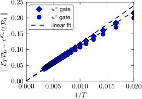
Figure 1: Robustness against dissipative errors. Distance from the exact evolution and the effective one as a function of $1/T.$ The unperturbed Lindbladian is of the form $\mathcal{L}_{0}=\sum_{\alpha}\gamma_{\alpha}\mathcal{L}^{\alpha}$, where $\mathcal{L}^{\alpha}$ is generated by a collective Lindblad operator $S^{\alpha}=\sum_{j=1}^{N}\sigma_{j}^{\alpha}$ with $N=4$. The control Hamiltonians are $\mathcal{K}^{\alpha}=-i\left[H^{\alpha},\bullet\right]$ with $H^{x}=(3/2)\left(\sigma_{1}^{z}\sigma_{2}^{z}+\sigma_{2}^{z}\sigma_{3}^{z}\right)+\openone$ and $H^{z}=-(\sqrt{3}/2)\left(\sigma_{1}^{z}\sigma_{2}^{z}-\sigma_{2}^{z}\sigma_{3}^{z}\right)+\sigma_{1}^{z}$. The effective dynamics generate the unitary gates $u^{\alpha}=\exp{(-i\theta\sigma^{\alpha})}$ with an arbitrary angle $\vartheta$ up to an error $O(T^{-1})$ (see also zanardi-dissipation-2014 ). The same dynamics is obtained (up to an error $O(T^{-1})$ with possibly a different prefactor) with an error on $\mathcal{L}_{0}$ which replaces $S^{\alpha}\to S^{\alpha}+T^{-1}X^{\alpha}$. For the numerical simulation we used $X^{\alpha}=g\bm{\sigma}_{1}\cdot\bm{\sigma}_{2}S^{z}$. The plot is obtained fixing $\gamma^{\alpha}=g=\vartheta=1$. The norm used is the maximum singular value of the maps realized as matrices over ${\cal H}^{\otimes\,2}.$ The linear fit is obtained using the four most significant points.

V Robustness

One of the main motivations behind the type of dissipation-assisted manipulations we are considering, is that it features a significant degree of built-in resilience. This means that dissipation, besides providing assistance for QIP, may provide protection. This stems from the simple observation that the projection theorem (2) clearly indicates that any extra term ${\cal V}$ in the Liouvillian, either Hamiltonian or dissipative, such that $\|{\cal V}\|=O(1/T)=$ and

$${\cal P}_{0}\,{\cal V}\,{\cal P}_{0}=0,$$ (16)

will not contribute to the effective dynamics (2). For instance in the context of Example 0 any pair of Hamiltonians $K_{1}$ and $K_{2}$ such that $\mathrm{Tr}_{B}[\rho_{B}(K_{1}-K_{2})]=\lambda\openone_{S},\,(\lambda\in{\mathbf{R}})$ generate the same projected dynamics.

V.1 Hamiltonian perturbations

In the Interaction Algebra case associated with the Liouvillian in Eq. (10), one can prove the following result which is reminiscent of the correctability condition in operator error correction OPC (see e.g., Eq. (4) therein). Proposition 2.– Eq.  (16) is satisfied by an Hamiltonian perturbation $V$ iff

$${\cal P}_{0}({V})\in{\cal A}\cap{\cal A}^{\prime}=:{\cal Z}({\cal A}).$$ (17)

The solution space of the Hamiltonian robustness Eq. (17) is a linear subspace of the full operator algebra ${\mathrm{L}}({\cal H})$ with codimension $\sum_{J}(n_{J}^{2}-1).$ This subspace, in particular, contains the kernel of ${\cal P}_{0}$ and the interaction algebra ${\cal A}.$

Proof.– From Eq. (15) we see that the condition (16), for ${\cal V}=-i[V,\bullet],$ means $[{\cal P}_{0}(V),\,\rho]=0,\,\forall\rho\in{\cal A}^{\prime},$ namely the projected dynamics does not change by perturbing $K$ with any term $V$ such that $\|V\|=O(1/T)$ and ${\cal P}_{0}(V)\in{\cal A}^{\prime\prime}={\cal A}.$ Since, by construction ${\cal P}_{0}(V)\in{\cal A}^{\prime}$ as well one finds that (16) is satisfied by an Hamiltonian perturbation $V$ iff Eq. (17) is satisfied. Moreover, if $V\in{\cal Z}({\cal A})\Rightarrow\,{\cal P}_{0}(V)=V$ implies that the solution space of Eq. (17) is the linear space ${\mathrm{Ker}}\,{\cal P}_{0}+{\cal Z}({\cal A}).$ More concretely, the Hamiltonian perturbations $V$ fulfilling the robustness condition Eq.  (17) have the form

$$V=V^{\textrm{off}}+\sum_{J\beta}X_{J}^{\beta}\otimes Y_{J}^{\beta}+\sum_{J}\lambda_{J}\openone_{n_{J}}\otimes\openone_{d_{J}}$$ (18)

where ${\mathrm{Tr}}(Y_{J}^{\beta})=0,\,(\forall J,\beta),$ and $V^{\textrm{off}}$is off-diagonal in the decomposition (13). The first two terms in the (18) represent ${\mathrm{Ker}}\,{\cal P}_{0}$ whose dimension is then $\sum_{J\neq J^{\prime}}(n_{J}d_{J})(n_{J}^{\prime}d_{J}^{\prime})+\sum_{J}n_{J}^{2}(d_{j}^{2}-1)=(\sum_{J}n_{J}d_{J})^{2}-\sum_{J}n_{J}^{2}={\mathrm{dim}}\,{\mathrm{L}}({\cal H})-{\mathrm{dim}}\,{\cal A}^{\prime}.$ The third term in (18) represent the center ${\cal Z}({\cal A})$ of the interaction algebra whose dimension is $\sum_{J}1.$ Overall we see that the solution space of (17) has dimension ${\mathrm{dim}}\,{\mathrm{L}}({\cal H})-\sum_{J}n_{J}^{2}+\sum_{J}1={\mathrm{dim}}\,{\mathrm{L}}({\cal H})-\sum_{J}(n_{J}^{2}-1)$ i.e., it has codimension $\sum_{J}(n_{J}^{2}-1).$ $\hfill\Box$ For example, in the collective decoherence case the interaction algebra $\cal A$ is the algebra of permutation-invariant operators acting on the $N$-qubit space DFS ; DFS1 . Since

$${\cal P}_{0}(\sigma_{j}^{\alpha}) = \int_{SU(2)}dUU^{\otimes\,N}\sigma_{j}^{\alpha}U^{\dagger\otimes\,N}=\int_{SU(2)}dUU\sigma_{j}^{\alpha}U^{\dagger}$$

$$= {\mathrm{Tr}}(\sigma_{j}^{\alpha})\,\openone=0\qquad(\alpha=x,y,z;\,j=1,\ldots,N),$$

it follows that all symmetry-breaking $V$’s of the form $V=\sum_{j=1.\alpha=x,y,z}^{N}\delta_{\alpha}^{j}\sigma_{j}^{\alpha}$ with $|\delta_{\alpha}^{j}|=O(1/T)$ can be tolerated.

V.2 Dissipative perturbations

Besides unitary perturbations $K\to K+V$ in practical applications one has also to consider dissipative ones ${\cal L}_{0}\to{\cal L}_{0}+{\cal L}_{1}$ where ${\cal L}_{1}$ denotes a dissipative Liouvillian with $\|{\cal L}_{1}\|=O(1/T).$ It is important to stress that the resilience of the projected dynamics extends to non-unitary perturbations e.g., extra noise sources.

To begin with, we observe that in the unit-preserving case all Lindbladian perturbations ${\cal L}_{1}$ of the form of Eq. (10) whose Lindblad operators are in the interaction algebra ${\cal A}$ [see Eq. (11], satisfy ${\cal P}_{0}{\cal L}_{1}{\cal P}_{0}=0$. Let us then consider perturbations that take the Lindblad operators outside of ${\cal A}$. More precisely, we consider Eq. (10) with Lindblad operators given by collective spin operators $S^{\mu}=\sum_{j=1}^{N}\sigma_{j}^{\mu}\,(\mu=x,y,z)$ and then we perturb them by permutational symmetry breaking terms ${S}^{\mu}\mapsto S^{\mu}+T^{-1}X^{\mu}$ where $\|X^{\mu}\|=O(1).$ This leads to a perturbed Liouvillian $\tilde{{\cal L}}_{0}={\cal L}_{0}+T^{-1}{\cal L}_{1}+T^{-2}{\cal L}_{2}.$ Where

$${\cal L}_{1}(\rho)=\sum_{\mu}\left(X^{\mu}\rho S^{\mu}+S^{\mu}\rho X^{\mu}-\frac{1}{2}\{\,\{X^{\mu},\,S^{\mu}\},\,\rho\}\right)$$ (19)

and ${\cal L}_{2}$ is a quadratic expression in the $X^{\mu}$’s. Proposition 3.– If ${\cal L}_{1}$ is given by (19) then ${\cal P}_{0}\,{\cal L}_{1}\,{\cal P}_{0}=0.$

Proof.– To see that is enough to notice that $\rho\in{\cal A}^{\prime}\Rightarrow\rho=\oplus_{J}\rho_{J}\otimes\openone_{d_{J}},$ and $S^{\mu}=\oplus_{J}\openone_{n_{J}}\otimes S_{J}^{\mu}.$ Since ${\cal P}_{0}$ annihilates any off-diagonal contribution in (19) one can assume a $J$ block-diagonal structure for the perturbation: $X^{\mu}=\oplus_{J}X_{J}^{\mu}\otimes Y_{J}^{\mu}.$ Therefore by considering, for example, the term ${\cal P}_{0}(X^{\mu}\rho S^{\mu})={\cal P}_{0}(X^{\mu}S^{\mu}\rho)={\cal P}_{0}(X^{\alpha}S^{\mu})\rho$ one obtains

$${\cal P}_{0}(X^{\mu}S^{\mu}) = {\cal P}_{0}\left(\oplus X_{J}^{\mu}\otimes Y_{J}S_{J}^{\mu}\right)=\oplus_{J}{\rm{Tr}}_{d_{J}}(Y_{J}S_{J}^{\mu})\,X_{J}^{\alpha}\otimes\openone/d_{J}$$ (20)

$$= \oplus_{J}{\rm{Tr}}_{d_{J}}(S_{J}^{\mu}Y_{J})\,X_{J}^{\mu}\otimes\openone/d_{J}={\cal P}_{0}(S^{\mu}X^{\mu}).$$

This shows that any term in ${\cal P}_{0}\,{\cal L}_{1}\,{\cal P}_{0}$ arising e.g., from the first term in (19), is canceled by an identical one arising from the anti-commutator side as ${\cal P}_{0}(X^{\mu}S^{\mu}\rho+S^{\mu}X^{\mu}\rho)=2{\cal P}_{0}(S^{\mu}X^{\mu})\rho.$ Notice that in particular for $X^{\mu}\in{\cal A}^{\prime}$ one has the stronger property ${\cal L}_{1}{\cal P}_{0}=0.$ $\hfill\Box$

In Fig. 1 we report a numerical simulation for the four qubits system discussed in the former section. The simulation confirms that for small $1/T$ the Liouvillians ${\cal L}_{0}$ and $\tilde{{\cal L}}_{0}$ generate the same projected dynamics zanardi-dissipation-2014 . In words: one can exploit (symmetric) noise to wash out other noise.

VI Emerging unitarity

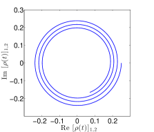
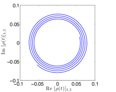
Figure 2: Unitarity from dissipation: a unitary dynamics is generated out of a purely dissipative one. To highlight the unitary character we use the method described in Q-BIO . For unitary dynamics one has $\rho(t)=e^{-itH_{\mathrm{eff}}}\rho_{0}e^{itH_{\mathrm{eff}}}=\sum_{n,m}e^{-it(E_{n}-E_{m})}\left[\rho_{0}\right]_{n,m}|n\rangle\langle m|$, with $H_{\mathrm{eff}}=\sum_{n}E_{n}|n\rangle\langle n|$. In the figure we plot the real and imaginary part of $\langle 1|\rho(t)|2\rangle$. Left panel: two qubit example generating the effective Hamiltonian $H_{eff}=\sigma^{y}\otimes\openone$. The time evolution window is $t\in[T/100,10T]$ and $T=100$ arbitrary units (AU). Right panel: four qubit example with perturbed collective noise. The effective Hamiltonian is given in Eq. 28. The time evolution window is $[T/2,4T]$ with $T=100$ AU.

A unitary dynamics gives rise to a non-unitary one as soon as some unobserved degrees of freedom are traced out. This is an ubiquitous situation in physics. The converse process, to obtain a unitary evolution from an underlying dissipative one, appears a much more difficult task. Here we show how this phenomenon of emerging unitarity manifests itself in the context we have discussed in this paper.

We begin by slightly generalizing our set-up i.e., going beyond the unital case where the kernel of ${\cal L}_{0}$ is the commutant of the interaction algebra. According to Ref  baum any generator of the Lindblad type (10) is such that its SSS is given by states $\rho$ of the form $\rho=\sum_{J}^{\oplus}\lambda_{J}\,\omega_{J}\otimes\rho_{0,J}$ where the state space block structure is still of the form (12). Here the $\omega_{J}$ are arbitrary states in ${\mathbf{C}}^{n_{J}},$ the $\rho_{0,J}$’s are uniquely defined states in ${\mathbf{C}}^{n_{J}}$ and the $\lambda_{J}$’s are non-negative scalars. In the unital case we mostly considered so far $\rho_{0,J}=\openone_{d_{J}}/d_{J}.$ The robustness calculation of the the former section can be now generalized to this non-unital Liouvillians case. As before we perturb the (not necessarily hermitean) Lindblad operators $L_{\alpha}\mapsto L_{\alpha}+\delta L_{\alpha}$ and consider as perturbation the first order variation of ${\cal L}_{0}.$

$${\cal L}_{1}(\rho)=\sum_{\alpha}(\delta L_{\alpha}\rho L_{\alpha}^{\dagger}-\frac{1}{2}(\delta L_{\alpha}^{\dagger}L_{\alpha}+L_{\alpha}^{\dagger}\delta L_{\alpha})\,\rho+{\mathrm{h.c.}})$$ (21)

If $\|\delta L_{\alpha}\|=O(1/T)$ then Eq. (2) holds with $\tilde{{\cal K}}$ replaced by ${\cal L}_{1}.$ Proposition 4.– Let us add, to a Liouvillian generator of the type (10), a perturbation of the form (21). Then, for $\rho$ in the SSS, one has that ${\cal P}_{0}{\cal L}_{1}{\cal P}_{0}(\rho)=-i[A,\,\rho],$ where

$$A={\mathrm{Im}}\,\sum_{\alpha}\sum_{J}^{\oplus}{\mathrm{Tr}}_{d_{J}}\left(\delta L_{\alpha}^{\dagger}L_{\alpha}\,(\openone_{n_{J}}\otimes\rho_{0,J})\right)\otimes\openone_{d_{J}}=A^{\dagger}$$ (22)

in which ${\mathrm{Im}}\,X:=\frac{1}{2i}(X-X^{\dagger}).$ In particular, for the unital case ${\cal L}_{0}(\openone)=0,$ one can write

$$A={\mathrm{Im}}\,{\cal P}_{0}\,(\sum_{\alpha}\delta L_{\alpha}^{\dagger}L_{\alpha}).$$ (23)

Proof.– Let us consider the Lindbladian ${\cal L}_{0}(\rho)=L\rho L^{\dagger}-\frac{1}{2}\{L^{\dagger}L,\,\rho\}.$ Perturbing the Lindblad operators $L\mapsto L+\delta L$ one finds the variation ${\cal L}_{0}\mapsto{\cal L}_{0}+\delta{\cal L},$ where

$$\delta{\cal L}(\rho)=\delta L\rho L^{\dagger}-\frac{1}{2}(L^{\dagger}\delta L+\delta L^{\dagger}L)\,\rho+{\mathrm{h.c}},$$ (24)

Without loss of generality we can consider $\delta L$ as block-diagonal in the decomposition (13) and work on a fixed $J$ sector ${\mathbf{C}}^{n_{J}}\otimes{\mathbf{C}}^{d_{J}}$. In that sector we write: $\delta L=X\otimes Y,$ $L=\openone\otimes\tilde{L}$ and $\rho=\omega\otimes\rho_{0}$ in the SSS. Here $\rho_{0}$ denotes the unique steady-state in the ${\mathbf{C}}^{d_{J}}$ factor of the $J$ block i.e., $\openone_{d_{J}}/d_{J}$ in the unital case. The first three terms in (24) give rise to the following three contributions respectively

$$X\omega\otimes Y\rho_{0}\tilde{L}^{\dagger},\;\;\;-\frac{1}{2}X\omega\otimes\tilde{L}^{\dagger}Y\rho_{0},\;\;\;-\frac{1}{2}X^{\dagger}\omega\otimes Y^{\dagger}\tilde{L}\,\rho_{0}.$$

Applying ${\cal P}_{0}\colon A\otimes B\mapsto{\mathrm{Tr}}(B)\,A\otimes\rho_{0}$ and adding the h.c., terms one finds

$${\cal P}_{0}\delta{\cal L}{\cal P}_{0}(\rho)=(\frac{\alpha}{2}X\omega-\frac{\bar{\alpha}}{2}X^{\dagger}\omega)\otimes\rho_{0}+{\mathrm{h.c.}}=$$

$$-i\,[\frac{\bar{\alpha}X^{\dagger}-{\alpha}X}{2i},\,\omega]\otimes\rho_{0},\quad\alpha:={\mathrm{Tr}}(\tilde{L}^{\dagger}Y\rho_{0}).$$ (25)

On the other hand $\delta L^{\dagger}L=(X^{\dagger}\otimes Y^{\dagger})(\openone\otimes\tilde{L})=X^{\dagger}\otimes Y^{\dagger}\tilde{L}$ from which we see that (25) can be written as $-i[\tilde{A},\,\omega\otimes\rho_{0}]$ where $\tilde{A}={\mathrm{Im}}\,{\mathrm{Tr}}_{d_{J}}\left(\delta L^{\dagger}L\,(\openone\otimes\rho_{0})\right)\otimes\openone_{d_{J}}.$ Here the index $d_{J}$ denotes the second factor i.e., ${\mathbf{C}}^{d_{J}}$ in the bipartition of the given $J$ block. Let us now consider a Liouvillian ${\cal L}_{0}$ with more than one Lindblad operator $\{L_{\alpha}\}_{\alpha}$. Putting together all the different $J$-blocks, we obtain ${\cal P}_{0}{\cal L}_{1}{\cal P}_{0}(\rho)=-i[A,\,\rho]$ where $A$ is given by Eq. (22) with $\rho=\sum_{J}^{\oplus}\omega_{J}\otimes\rho_{0,J},\,({\cal P}_{0}(\rho)=\rho).$ In the unital case one has $\rho_{0,,J}={\openone_{d_{J}}}/{d_{J}}$ and Eq. (23) follows from (22) and (14).$\hfill\Box$ Corollary i) If all the $L_{\alpha}$’s and perturbations $\delta L_{\alpha}$’s are Hermitean $A=0;$ ii) If $\delta L_{\alpha}\in{\cal A}^{\prime}(\Rightarrow(X_{\alpha})_{J}\sim\openone_{n_{J}})$ then $A_{J}\sim\openone_{n_{J}}\Rightarrow{\cal P}_{0}\delta{\cal L}{\cal P}_{0}=0.$

While mathematically simple the Proposition 4 is, on physical grounds, a remarkable and surprising result. Combined with the dissipation-projection theorem Eq. (2), it indeed implies that a small, generic, Lindblad perturbation induces an effective unitary dynamics over the SSS generated by the Hamiltonian (22). This even in absence of any Hamiltonian term in both the unperturbed and unperturbed Liouvillian. In principle, by tailoring the dissipative terms $\delta L_{\alpha}$’s, one can obtain a desired effective unitary generator $A.$

VI.1 Examples

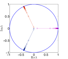
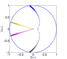
Figure 3: Unitarity from dissipation: a unitary dynamics is generated out of a purely dissipative one. Here we plot real and imaginary part of the eigenvalues of the exact map $\mathcal{E}_{T}{\cal P}_{0}=\exp\left[T(\mathcal{L}_{0}+\frac{1}{T}{\cal L}_{1}+\frac{1}{T^{2}}{\cal L}_{2})\right]{\cal P}_{0}$ for different $T$. The examples are the same as in Fig. 2, i.e. two (four) qubit example on the left (right) panel. Increasing $T$ the eigenvalues tend to go on the unit circle. Left panel: $T\in[1,1000]$ AU, the eigenvalues approach $e^{\pm 2i},1$, consistently with Eq. (26). Right panel: $T\in[5,600]$ AU. The eigenvalues of the effective Hamiltonians (28) are $\pm 8,0$. Consequently the eigenvalues of $\mathcal{E}_{T}P_{0}$ approach $e^{\pm 16i},e^{\pm 8i},1$.

To illustrate this mechanism we first consider a simple two-qubit example. We set $L=\openone\otimes\sigma^{z}$ and $\delta L=\sigma^{-}\otimes\sigma^{z}.$ In this case ${\cal P}_{0}(X)={\mathrm{Tr}}_{B}\left(X(\openone\otimes|0\rangle\langle 0|)\right)\otimes|0\rangle\langle 0|+{\mathrm{Tr}}_{B}\left(X(\openone\otimes|1\rangle\langle 1|)\right)\otimes|1\rangle\langle 1|,$ where ${\mathrm{Tr}}_{B}$ denotes the partial trace over the second qubit. Using Eqs. (25), (22) with $J=0,1;\,d_{0}=d_{1}=1;\,\rho_{0,0}=|0\rangle\langle 0|,\,\rho_{0,1}=|1\rangle\langle 1|;\,X=\sigma^{-}$ and $Y=\sigma^{z}$ one finds

$$A={\mathrm{Im}}\,{\cal P}_{0}(\delta L^{\dagger}L)=\sigma^{y}\otimes|0\rangle\langle 0|+\sigma^{y}\otimes|1\rangle\langle 1|=\sigma^{y}\otimes\openone.$$ (26)

A numerical simulation of this dissipation generated gate is shown in Figs. 2, 3 left panel. To highlight the unitary character of the dynamics we use the fact that matrix elements of the density matrix $\rho(t)$ evolve as phases in the Hamiltonian eigenbasis and therefore result in circles on the complex plane [Fig. 2]. Similarly as $\mathcal{E}_{T}$ approaches a unitary evolution within the SSS, the eigenvalues of $\mathcal{E}_{T}\mathcal{P}_{0}$ converge to the unit circle increasing $T$ as depicted in Fig. 3.

Let us now consider a four-qubit system subject to general collective decoherence DFS ; DFS1 . In this case ${\cal L}_{0}$ has the form (10) with the Lindblad operators given by collective spin operators i.e., $L_{\alpha}=\sum_{j=1}^{4}\sigma_{j}^{\alpha},\,(\alpha=x,y,z).$ In this unital case the interaction algebra ${\cal A}$ coincides with algebra of totally symmetric operators and the commutant ${\cal A}^{\prime}$ is $14-$dimensional zanardi-dissipation-2014 and generated by qubit permutation operators in the group ${\cal S}_{4}$. We consider perturbations of the form $\delta L_{\alpha}=U\,{L}_{\alpha}=L_{\alpha}\,U$ where $U\in{\cal S}_{4}.$ Then $\sum_{\alpha}\delta L_{\alpha}^{\dagger}L_{\alpha}=4U^{\dagger}\bm{S}^{2}$, where $\bm{S}$ is the total spin operator. We also have $\mathcal{P}_{0}\left(U^{\dagger}\bm{S}^{2}\right)=U^{\dagger}\bm{S}^{2}$ and $U^{\dagger}\bm{S}^{2}-U\bm{S}^{2}=2(U^{\dagger}-U)$. We further fix $U$ to perform the right-shift permutation $\left(1,2,3,4\right)\to\left(4,1,2,3\right)$. One obtains

$$A =4\,\mathrm{Im}\,\mathcal{P}_{0}\left(U^{\dagger}\bm{S}^{2}\right)=8\,\mathrm{Im}(U^{\dagger})$$ (27)

$$=\left[(\bm{\sigma}_{1}+\bm{\sigma}_{2})\times\bm{\sigma}_{3}\right]\cdot\bm{\sigma}_{4}+\left[\bm{\sigma}_{2}\times(\bm{\sigma}_{3}+\bm{\sigma}_{4})\right]\cdot\bm{\sigma}_{1}\,,$$ (28)

where in the last equation we used the fact that $U=S_{2,3}S_{3,4}S_{1,4}$ with $S_{i,j}=\left(\openone+\bm{\sigma}_{i}\cdot\bm{\sigma}_{j}\right)/2$ the operator swapping site $i$ with $j$. A numerical simulation confirming this unitary behavior emerging from a dissipative dynamics, is shown in Figs. 2,3 right panel.

VII Conclusions

The traditional avenue to quantum information processing (QIP) primitives, such as quantum gates, requires the dissipation due to the environment to be as small a possible compared to the control Hamiltonian. A number of powerful techniques have been develop to combat the detrimental effects of dissipation QEC . However, over the last few years there has been a growing amount of evidence that dissipation may on the contrary provide a resource for QIP see e.g., Kraus-prep ; kastoryano2011dissipative ; barreiro2011open ; verstraete2009quantum ; dissi-top ; gauge .

In this spirit in ref. zanardi-dissipation-2014 we have shown how it is possible to generate coherent quantum manipulations also in the opposite regime in which the dissipation is much stronger than the control Hamiltonian. The only requirement is essentially that the dissipation must provide a degenerate set of steady states (SSS). The coherent control drives the system away from the SSS but the strong dissipation effectively projects the dynamics back onto the SSS. As a consequence a quantum evolution governed by an effective Hamiltonian coherently unfolds within the SSS zanardi-dissipation-2014 .

In this paper we further investigated the consequences of this approach. The following are the main findings of this paper. i) We provided further details on the rigorous estimate of the error between the exact evolution and the effective projected dynamics. ii) Moving to a suitable rotated frame, we have shown that the effective dynamics in the SSS is of geometric origin i.e., it is the holonomy associated with a superoperator-valued connection. iii) The effective dynamics is protected against a large class of Hamiltonian and dissipative perturbations. iv) As a corollary of this result, we have shown that certain dissipative perturbations of purely, dissipative, Lindbladian (i.e. one for which the eigenvalues are real negative) generate an effective unitary dynamics.

Dissipative dynamics is easily obtained from a unitary one as soon as some degrees of freedom are traced out. On the contrary the emergent unitarity phenomenon we have discussed is a quite surprising example of a unitary dynamics obtained from a purely dissipative one. Understanding its fundamental origin and potential application in QIP is a topic worthwhile of future investigations.

Appendix A Error estimate

Here we are going to estimate the error term appearing in the RHS of Eq. (2). In this section we use the following notation for the total Liouvillian: $\mathcal{L}(x)=\mathcal{L}_{0}+x\mathcal{L}_{1}$, where $\mathcal{L}_{0}$ is the dominant, dissipative, term, $\mathcal{L}_{1}$ is the perturbation (which often will be taken as a unitary generator, i.e. $\mathcal{L}_{1}=\mathcal{K}$), and $x$ is a small dimensionless parameter. The relation between $x$ and the $T$ in the main text is $T^{-1}=x\tau_{0}^{-1}$ where $\tau_{0}$ is some time-scale which will become more explicit below. We are going to show that the LHS of Eq. (2) is analytic in $x$ around zero starting with a linear term and we are going to estimate its coefficient. Let us assume that $\mathrm{Ker}(\mathcal{L}_{0})$ is $d$-dimensional, i.e. $d$ eigenvalues of $\mathcal{L}_{0}$ are zero. If we turn on the perturbation $x\mathcal{L}_{1}$, some of these eigenvalues will move a little bit. The collection of all these $d$ eigenvalues forms the so called $\lambda$-group kato and identifies an invariant subspace of $\mathcal{L}(x)$. The projection $\mathcal{P}(x)$ onto such subspace turns out to be an analytic function of $x$ kato . As shown in kato , the restriction of $\mathcal{L}(x)$ to the $\lambda$-group, $\mathcal{R}(x):=\mathcal{P}(x)\mathcal{L}(x)=\mathcal{L}(x)\mathcal{P}(x)=\mathcal{P}(x)\mathcal{L}(x)\mathcal{P}(x)$, is also an analytic function of $x$. Then one has the following expansions

$$\mathcal{P}(x) = \mathcal{P}_{0}+x\mathcal{P}_{1}+O(x^{2})$$ (29)

$$\mathcal{R}(x) = x\mathcal{R}_{1}+x^{2}\mathcal{R}_{2}+x^{3}\mathcal{R}_{3}+O(x^{4}).$$ (30)

The Liouvillian character of $\mathcal{L}_{0}$ (i.e. that fact that $\mathcal{P}_{0}=\lim_{t\to\infty}e^{t\mathcal{L}}$) assures that zero is a semisimple eigenvalue of $\mathcal{L}_{0}$, i.e. there is no Jordan block associated with the zero eigenvalue of $\mathcal{L}_{0}$. Whereas this is not strictly required it does simplify the following formulae. In the semisimple case one has for instance kato :

$$\mathcal{P}_{1} =-(\mathcal{P}_{0}\mathcal{L}_{1}\mathcal{S}+\mathcal{S}\mathcal{L}_{1}\mathcal{P}_{0})$$ (31)

$$\mathcal{R}_{1} =\mathcal{P}_{0}\mathcal{L}_{1}\mathcal{P}_{0}$$ (32)

$$\mathcal{R}_{2} =-\left(\mathcal{P}_{0}\mathcal{L}_{1}\mathcal{P}_{0}\mathcal{L}_{1}\mathcal{S}+\mathcal{P}_{0}\mathcal{L}_{1}\mathcal{S}\mathcal{L}_{1}\mathcal{P}_{0}+\mathcal{S}\mathcal{L}_{1}\mathcal{P}_{0}\mathcal{L}_{1}\mathcal{P}_{0}\right).$$ (33)

In the above formulae, $\mathcal{S}$ is the projected resolvent of $\mathcal{L}_{0}$ at zero satisfying $\mathcal{L}_{0}\mathcal{S}=\mathcal{S}\mathcal{L}_{0}=\openone-\mathcal{P}_{0}$ and is given by

$$\mathcal{S}=-\sum_{k\neq 0}\left[(-\lambda_{k})^{-1}\mathcal{P}^{(k)}+\sum_{n=1}^{m_{k}-1}(-\lambda_{k})^{-n-1}\left(\mathcal{D}^{(k)}\right)^{n}\right],$$ (34)

assuming that $\mathcal{L}_{0}$ has Jordan decomposition

$$\mathcal{L}_{0}=\sum_{k}\left(\lambda_{k}\mathcal{P}^{(k)}+\mathcal{D}^{(k)}\right)$$ (35)

with $\lambda_{k}$ eigenvalues with (algebraic) multiplicity $m_{k}$, projectors $\mathcal{P}^{(k)}$ and nilpotent blocks $\mathcal{D}^{(k)}$ (note that $\lambda_{0}=0$ and $\mathcal{P}^{(0)}\equiv\mathcal{P}_{0}$). Note that all the $\mathcal{L}_{j},\,\mathcal{R}_{j}^{\prime}s$ have the dimension of Hz, the $\mathcal{P}_{j}$’s are dimensionless and $\mathcal{S}$ has units of time. In particular $tx\mathcal{R}_{1}$ is precisely $\mathcal{L}_{\mathrm{eff}}$ in our applications. We denote it $\mathcal{R}_{eff}:=tx\mathcal{R}_{1}$ here for notational consistency.

Clearly $\mathcal{P}(x)$ commutes with $\mathcal{L}(x)$ and so one has the identity

$$e^{t\mathcal{L}(x)}\mathcal{P}(x)=e^{t\mathcal{R}(x)}\mathcal{P}(x).$$ (36)

We now choose times $t$ such that $tx$ is bounded by a given finite time in some unit, i.e. $tx=O(1)\tau_{0}$. Note that $\left\|e^{t\mathcal{L}(x)}\right\|\leq 1$ because the evolution maps states to states (i.e. because of positivity). Instead from $\left\|e^{t\mathcal{R}(x)}\right\|\leq\exp\left\|t\mathcal{R}(x)\right\|$ we get $\left\|e^{t\mathcal{R}(x)}\right\|\leq O(1)$. Hence we obtain

$$\left(e^{t\mathcal{L}(x)}-e^{t\mathcal{R}(x)}\right)\mathcal{P}_{0}=-\left(e^{t\mathcal{L}(x)}-e^{t\mathcal{R}(x)}\right)x\mathcal{P}_{1}+O(x^{2}).$$ (37)

Now define $\Delta=:e^{tx\mathcal{R}_{1}}-e^{t\mathcal{R}(x)}$. Clearly $\Delta=O(x)$ (we will later determine the coefficient), so we finally get

$$\left(e^{t\mathcal{L}(x)}-e^{tx\mathcal{R}_{1}}\right)\mathcal{P}_{0}=+\Delta\mathcal{P}_{0}-\left(e^{t\mathcal{L}(x)}-e^{tx\mathcal{R}_{1}}\right)x\mathcal{P}_{1}+O\left(x^{2}\right).$$ (38)

Using Dyson expansion one can easily estimate $\Delta$:

$$\Delta=tx^{2}\int_{0}^{1}e^{(1-s)\mathcal{R}_{eff}}\mathcal{R}_{2}e^{s\mathcal{R}_{eff}}ds+O\left(x^{2}\right).$$

Quite naturally we use a submultiplicative and automorfism-invariant norm for superoperators. We now take the norm of Eq. (38), use triangle inequality and bound all the resulting terms. Defining $C=\sup_{s\in\left[0,1\right]}\left\|e^{s\mathcal{R}_{\mathrm{eff}}}\right\|$, we get $\left\|\Delta\right\|\leq tx^{2}C^{2}\left\|\mathcal{R}_{2}\right\|+O(x^{2})$, $\left\|\mathcal{R}_{2}\right\|\leq 3\left\|\mathcal{P}_{0}\right\|^{2}\left\|\mathcal{L}_{1}\right\|^{2}\left\|S\right\|$, and $\left\|\mathcal{P}_{1}\right\|\leq 2\left\|\mathcal{P}_{0}\right\|\left\|\mathcal{L}_{1}\right\|\left\|S\right\|$. Putting things together we finally obtain

$$\left\|\left(e^{t\mathcal{L}(x)}-e^{\mathcal{R}_{\mathrm{eff}}}\right)\mathcal{P}_{0}\right\|\leq x\left\|\mathcal{S}\right\|\left\|\mathcal{L}_{1}\right\|\left\|\mathcal{P}_{0}\right\|\\ \times\left(3txC^{2}\left\|\mathcal{P}_{0}\right\|^{2}\left\|\mathcal{L}_{1}\right\|+4\right)+O(x^{2}).$$ (39)

In order to make more apparent the connection with physical constants, we define dimensionless (tilded) operators via $\mathcal{L}=\gamma_{0}\tilde{\mathcal{L}}_{0}+\gamma_{1}\tilde{\mathcal{L}}_{1}$ such that $\gamma_{0}^{-1}=\tau_{R}$ is the (short) relaxation time of the unperturbed dissipation and $\gamma_{1}^{-1}=T$ is the timescale of the control term. Measuring times in units of $\tau_{R}$ the evolution becomes $\exp\left[(t/\tau_{R})\left(\tilde{\mathcal{L}}_{0}+x\tilde{\mathcal{L}}_{1}\right)\right]$ and we see that $x=\gamma_{1}/\gamma_{0}=\tau_{R}/T$ is the small parameter. The requirement that the effective generator $\tilde{\mathcal{R}}_{\mathrm{eff}}=t\gamma_{1}\tilde{\mathcal{P}}_{0}\tilde{\mathcal{L}}_{1}\tilde{\mathcal{P}}_{0}$ is finite and non-zero implies $t\gamma_{0}x=t\gamma_{1}=O(1)$. This means that the waiting time is given by $t=O(T)$. The bound Eq. (39) then translates into (all the tilded operators are dimensionless)

$$\left\|\left(e^{t\mathcal{L}}-e^{\tilde{\mathcal{R}}_{\mathrm{eff}}}\right)\mathcal{P}_{0}\right\|\leq\frac{\tau_{R}}{T}\left\|\tilde{\mathcal{S}}\right\|\left\|\tilde{\mathcal{L}}_{1}\right\|\left\|\tilde{\mathcal{P}}_{0}\right\|\\ \times\left(3\frac{t}{T}C^{2}\left\|\tilde{\mathcal{P}}_{0}\right\|^{2}\left\|\tilde{\mathcal{L}}_{1}\right\|+4\right)+O(x^{2}).$$ (40)

Equation above can often be further simplified. For example, if $\mathcal{L}_{0}$ generate a positive map $\left\|\tilde{\mathcal{P}}_{0}\right\|=1$, whereas if $\mathcal{R}_{\mathrm{eff}}$ generates a unitary one has $C=1$.

References

• (1) Quantum Error Correction. D. A. Lidar, T. Brun Eds. Cambridge University Press (2013)
• (2) P. Zanardi and M. Rasetti, Noiseless quantum codes Phys. Rev. Lett. 79, 3306 (1997); P. Zanardi, Decoherence and dissipation in a quantum register, Phys. Rev. A 57, 3276 (1998);
• (3) D. A. Lidar, I. L. Chuang, and K. B. Whaley, Decoherence free subspaces for quantum computation, Phys. Rev. Lett. 81, 2594 (1998).
• (4) D. Kielpinski et al, A Decoherence-Free Quantum Memory Using Trapped Ions, Science 291, 1013 (2001);
• (5) E. Knill, R. Laflamme, and L. Viola, Theory of quantum error correction for general noise, Phys. Rev. Lett. 84, 2525 (2000).
• (6) P. Zanardi, Stabilizing quantum information, Phys. Rev. A 63, 012301 (2000).
• (7) P. Zanardi, S. Lloyd, Topological protection and noiseless quantum subsystems, Phys. Rev. Lett 90, 067902 (2003)
• (8) L. Viola et al, Experimental realization of noiseless subsystems for quantum information processing, Science 293, 2059 (2001)
• (9) Jones, J. A., Vedral, V., Ekert, A. Castagnoli, G. Geometric quantum computation using nuclear magnetic resonance, Nature 403, 869 (2000)
• (10) P. Zanardi and M. Rasetti, Holonomic quantum computation, Phys. Lett. A 264, 94 (1999)
• (11) Duan, L. M., Cirac, J. I. Zoller, P. ,Geometric manipulation of trapped ions for quantum computation, Science 292, 1695 (2001)
• (12) B. Kraus, H. P. Büchler, S. Diehl, A. Kantian, A. Micheli, and P. Zoller, Preparation of entangled states by quantum Markov processes, Phys. Rev. A 78, 042307 (2008)
• (13) M. J. Kastoryano, F. Reiter, and A. S. Sorensen, Dissipative preparation of entanglement in optical cavities, Phys. Rev. Lett. 106, 090502 (2011).
• (14) J. T. Barreiro et al , An open-system quantum simulator with trapped ions, Nature (London) 470, 486 (2011).
• (15) F. Verstraete, M.M. Wolf,and J.I. Cirac, Quantum computation and quantum-state engineering driven by dissipation, Nat .Phys.5, 633 (2009).
• (16) C-E. Bardyn et al, Topology by dissipation, New J. Phys. 15, 085001 (2015)
• (17) K. Stannigel, P. Hauke, D. Marcos, M. Hafezi, S. Diehl, M. Dalmonte, P. Zoller, Constrained dynamics via the Zeno effect in quantum simulation: Implementing non-Abelian lattice gauge theories with cold atoms, Phys. Rev. Lett. 112, 120406 (2014)
• (18) P. Zanardi, L. Campos Venuti, Coherent quantum dynamics in steady-state manifolds of strongly dissipative systems, Phys. Rev. Lett. 113, 240406 (2014)
• (19) P. Facchi and S. Pascazio, Quantum Zeno Subspaces, Phys. Rev. Lett. 89, 080401 (2002).
• (20) G. A. Paz-Silva, A. T. Rezakhani, J. M. Dominy, and D. A. Lidar, Zeno effect for quantum computation and control, Phys. Rev. Lett. 108, 080501 (2012)
• (21) J. Pachos, P. Zanardi, and M. Rasetti, Non-Abelian Berry connections for quantum computation. Phys. Rev. A, 61:010305(R), (1999).
• (22) O. Oreshkov, J. Calsamiglia, Adiabatic markovian dynamics, Phys. Rev. Lett. 105, 050503 (2010)
• (23) A. Carollo, M. F. Santos, V. Vedral, Coherent quantum evolution via reservoir driven holonomies, Phys. Rev. Lett. 96, 020403 (2006)
• (24) M. Nakahara, Geometry, Topology and Physics, IOP Publishing Ltd., 1990
• (25) D. Burgarth, P. Facchi, V. Giovannetti, H. Nakazato, S. Pascazio, K. Yuasa, Exponential Rise of Dynamical Complexity in Quantum Computing through Projections, Nat. Comm. 5, 5173 (2014)
• (26) Y. Li, D. Herrera-Marti, L. C. Kwek, Quantum Zeno Effect of General Quantum Operations, arXiv:1305.2464
• (27) D. Burgarth et al, Non-Abelian Phases from a Quantum Zeno Dynamics, Phys. Rev. A 88, 042107 (2013).
• (28) G. Lindblad, On the generators of quantum dynamical semigroups, Commun. Math. Phys. 48, 119 (1976)
• (29) D. W. Kribs, Quantum channels, wavelets, dilatations and representations of $\mathcal{O}_{n}$, Proc. Edin. Math. Soc. 46 (2003)
• (30) P. Zanardi, Symmetrizing evolutions, Phys. Lett. A 258 77 (1999); P. Zanardi, Computation on an error-avoiding quantum code and symmetrization, Phys. Rev. A 60 729 (1999);
• (31) L. Viola, E. Knill, S. Lloyd, Dynamical decoupling of open quantum systems, Phys. Rev. Lett. 82, 2417 (1999)
• (32) K. Khodjasteh and D. A. Lidar, Fault Tolerant Quantum Dynamical Decoupling, Phys. Rev. Lett. 95, 180501 (2005)
• (33) G. Uhrig, Keeping a Quantum Bit Alive by Optimized $\pi$-Pulse Sequences, Phys. Rev. Lett. 98, 100504 (2007)
• (34) D. Kribs, R. Laflamme, D. Poulin, Unified and Generalized Approach to Quantum Error Correction, Phys. Rev. Lett. 94, 180501 (2005)
• (35) Lorenzo Campos Venuti and Paolo Zanardi, Excitation Transfer through Open Quantum Networks: Three Basic Mechanisms, Phys.Rev. B 84, 134206 (2011)
• (36) B. Baumgartner and H. Narnhofer, Analysis of quantum semigroups with GKS-Lindblad generators: II. General, J. Phys. A 41, 395303 (2008)
• (37) T. Kato, Perturbation Theory for Linear Operators, Springer 1995