Multi-filter transit observations of WASP-39b and WASP-43b
with three San Pedro Mártir telescopes

Abstract

Three optical telescopes located at the San Pedro Mártir National Observatory were used for the first time to obtain multi-filter defocused photometry of the transiting extrasolar planets WASP-39b and WASP-43b. We observed WASP-39b with the $2.12$ telescope in the $U$ filter for the first time, and additional observations were carried out in the $R$ and $I$ filters using the $0.84$ telescope. WASP-43b was observed in $VRI$ with the same instrument, and in the $i$ filter with the robotic $1.50$ telescope. We reduced the data using different pipelines and performed aperture photometry with the help of custom routines, in order to obtain the light curves. The fit of the light curves ($1.5$–$2.5\mathrm{m}\rm mag$ rms), and of the period analysis, allowed a revision of the orbital and physical parameters, revealing for WASP-39b a period ($4.0552947\pm 9.65\times 10^{-7}$ days) which is $3.084\pm 0.774$ seconds larger than previously reported. Moreover, we find for WASP-43b a planet/star radius ($0.1738\pm 0.0033$) which is $0.01637\pm 0.00371$ larger in the $i$ filter with respect to previous works, and that should be confirmed with additional observations. Finally, we confirm no evidence of constant period variations in WASP-43b.

1 Introduction

Since the first detection of an exoplanet orbiting around a pulsar (Wolszczan & Frail 1992; Wolszczan 1994) and around a main sequence star (Mayor & Queloz 1995) using radial velocity measurements, several other techniques, such as microlensing, coronagraphy, and polarimetric observations have been developed for the search of other worlds. Transit observations have contributed to a large fraction of the about $1\,800$ confirmed planets. Several systematic surveys have been implemented for the detection of exoplanet candidates by transit observations.

Important examples of these surveys include space-based missions such as CoRoT (Baglin et al. 2009) and Kepler (Borucki et al. 2010) satellites. The high photometric precision of their observations allowed to boost the number of candidates and confirmed extrasolar planets detected in the last five years. The next generation of space-based missions, such as the orbiting GAIA (Baglin & Catala 2009) and the upcoming JWST (Clampin 2008; Batalha et al. 2014), PLATO (Rauer et al. 2013), and TESS (Ricker et al. 2010) are expected to increase the detection rate, and broaden the limits of the currently observed distribution of exoplanetary parameters, despite that some of these missions have not the detection of exoplanets as a main goal.

On the other hand, ground-based photometric surveys such as SuperWASP (Pollacco et al. 2006) and HAT (Bakos et al. 2007) are focused on exoplanets with large radii and orbiting close to their host star, as these objects are particularly suited for these instruments. In order to improve the photometric precision of ground-based follow-up observations of exoplanetary transits, a technique consisting in slightly defocusing the image has been introduced and widely used in recent works (Southworth et al. 2009a, b, 2010, 2012b, 2013, 2014). The achieved results often compete with those of space-based surveys, and increase the opportunity for small telescopes to produce light curves with a remarkable photometric precision.

Following the results obtained with the defocused photometry technique, we started an observational campaign of known exoplanetary transits, already detected by the SuperWASP and HAT surveys. Photometric follow-up of these objects in different bandpasses is useful to study a possible dependence of the planetary radius as a function of the wavelength.

This project makes use of all three telescopes operating at the San Pedro Mártir National Astronomical Observatory (see Sect. 2 for details), which we employ for the first time in the field of transit observations. In this paper we focus on two particular targets: WASP-39b (catalog ) and WASP-43b (catalog ), which are briefly presented in the following subsections.

Table 1: Features of the three San Pedro Mártir telescopes and CCD detectors used for the observation of WASP-39b and WASP-43b.

Diameter	focal ratio	CCD size	Resolution	Field of View	Read Out Noise	Gain
$0.84$	$f/15.0$	$2043\times 4612$ px	$0.25\arcsec/$px	$8.4\arcmin\times 19.0\arcmin$	$\;\;4.8\rm e^{-}$	1.8
$1.50$	$f/13.0$	$1040\times 1056$ px	$0.32\arcsec/$px	$5.6\arcmin\times\;\;5.6\arcmin$	$11.3\rm e^{-}$	4.0
$2.12$	$f/13.5$	$2048\times 2048$ px	$0.18\arcsec/$px	$6.2\arcmin\times\;\;6.2\arcmin$	$\;\;4.5\rm e^{-}$	1.8

1.1 WASP-39b

WASP-39b is a Saturn-mass planet recently discovered by the SuperWASP survey, and confirmed by Faedi et al. (2011) with a photometric and spectroscopic follow-up observations. The photometry was carried on with the Pan-STARRS-$z$ filter on the the $2$ Faulkes telescope North, and in the Gunn-$i$ filter on the $1.2$ Euler telescope. The spectroscopy was carried out with the SOPHIE (Perruchot et al. 2008) and the CORALIE (Baranne et al. 1996; Queloz et al. 2000) spectrographs, installed on the $1.93$ telescope at the Haute-Provence Observatory (OHP) and on the $1.2$ Euler telescope, respectively.

Faedi et al. (2011) obtain a period of $P=4.055259$ days, a $T_{0}=2\,455\,342.9688$ in Heliocentric Julian Date (HJD), a transit duration of $168.192$ minutes, and the following physical parameters: a mass of $0.28M_{J}$, a radius of $1.27R_{J}$, and thus a resulting mean density of $0.14\rho_{J}$. This is one of the lowest values for the currently known extrasolar planets. The reported semi-major axis is $0.0486$ AU, and evidences of a highly inflated radius are also found.

This work presents the first photometric follow-up of WASP-39b since the discovery.

1.2 WASP-43b

WASP-43b is a very short-period hot Jupiter-like planet discovered by Hellier et al. (2011) using observations from the WASP-South camera array, complemented with photometric observations with the $0.6$ TRAPPIST telescope in the $I+z$ band and the Euler telescope in the Gunn $r$ band. Radial velocity measurements were also obtained with CORALIE. Hellier et al. (2011) find a period of $P=0.813475$ days, an initial epoch of $T_{0}=2\,455\,528.86774$ HJD, and a duration of $69.552$ min. The authors derive a mass of $1.8M_{J}$, a radius of $0.9R_{J}$ leading to a density of $2.21\rho_{J}$. The reported semi-major axis is $0.0142$ AU.

In order to improve the characterization of WASP-43b and its host star, for which Husnoo et al. (2012) find evidences of excess rotation, Gillon et al. (2012) observed over thirty eclipses between transits and occultations, using mainly the TRAPPIST telescope in the $I+z$ and $z$ bands, respectively. The survey was completed with transit observations obtained with the Euler telescope in the Gunn $r^{\prime}$ band and with the VLT/HAWK-I instrument installed on the $8.2$ UT4 telescope in Paranal. The work allowed significant improvements in the determination of the stellar density and in the refinement of the parameters of the planetary system. In particular, Gillon et al. (2012) find a mass of $2.034M_{J}$ and a radius of $1.036R_{J}$. Occultations also detected the thermal emission of the planet.

Thermal emission is also the subject of Spitzer observations, carried out by Blecic et al. (2012, 2014), which highlighted the possibility of thermal inversion in the atmosphere.

Line et al. (2014) uniformly analyzed occultations of nine exoplanets including WASP-43b, with the goal to characterize their $\rm C$ to $\rm O$ ratio, which is found to be $>1$ in the case of WASP-43b, and which is attributed to the upper limit value of $\rm CH_{4}$.

Other observations using the GROND instrument on the MPG/ESO $2.2$ telescope in the $g^{\prime}$, $r^{\prime}$, $i^{\prime}$, $z^{\prime}$, $J$, $H$, and $K$ bands (Chen et al. 2014) allowed to refine the period to a value of $P=0.81347437$. This value agrees with spectroscopic observations carried on by Murgas et al. (2014). These observations also confirmed planetary dayside thermal emission with poor heat redistribution, as observed by Wang et al. (2013b, a).

Table 2: Log of the observations of WASP-39b and WASP-43b.

Date	Filter	Exp.	Telescope
	WASP-39b
2014-03-17	$U$	$240$–$300$	$2.12$
2014-03-17	$I$	$120$–$180$	$0.84$
2014-03-21	$R$	$120$	$0.84$
	WASP-43b
2014-02-13	$R$	$60$–$120$	$0.84$
2014-03-07	$i$	$140$	$1.50$
2014-03-07	$R$	$60$	$0.84$
2014-03-20	$I$	$60$–$120$	$0.84$
2014-03-21	$V$	$60$–$120$	$0.84$
2014-03-29	$i$	$90$	$1.50$
2014-05-12	$I$	$60$–$120$	$0.84$

Finally, an X-ray study by Czesla et al. (2013) on the host star of WASP-43b using XMM-Newton observations found that the planet is exposed to a high-energy radiation field; and water abundance measurements were recently reported by Kreidberg et al. (2014).

In Sect. 2 we describe the used telescopes and our observations of WASP-39b and WASP-43b, while in Sect. 3 and 4 we focus on data reduction techniques and on a discussion about the period of the two objects. Results are presented in Sect. 5, while conclusions are described in Sect. 6.

2 Observations

Observations were carried on using all three equatorial Ritchey-Chrétien telescopes installed at the the San Pedro Mártir National Astronomical Observatory (SPM-OAN). These facilities are located at an altitude of $2\,800$ in the middle of the peninsula of Baja California in northwestern Mexico (N $31\mathrm{°}⁤02\mathrm{\prime }⁤39\mathrm{″}$, W $115\mathrm{°}⁤27\mathrm{\prime }⁤49\mathrm{″}$). The $0.84$ and the $2.12$ are operated on-site, and the $1.50$ is a robotic telescope monitored and operated remotely.

We principally used the $0.84$ telescope, an $f/15$ which provides an $8.4\arcmin\times 19.0\arcmin$ field of view on the Mexman instrument. We decided to window the Esopo CCD to avoid vignetting and to reduce the readout time. The instrument comes with a set of standard $UBVRI$ Johnson filters among others. In this paper we present observations carried out using the $VRI$ filters.

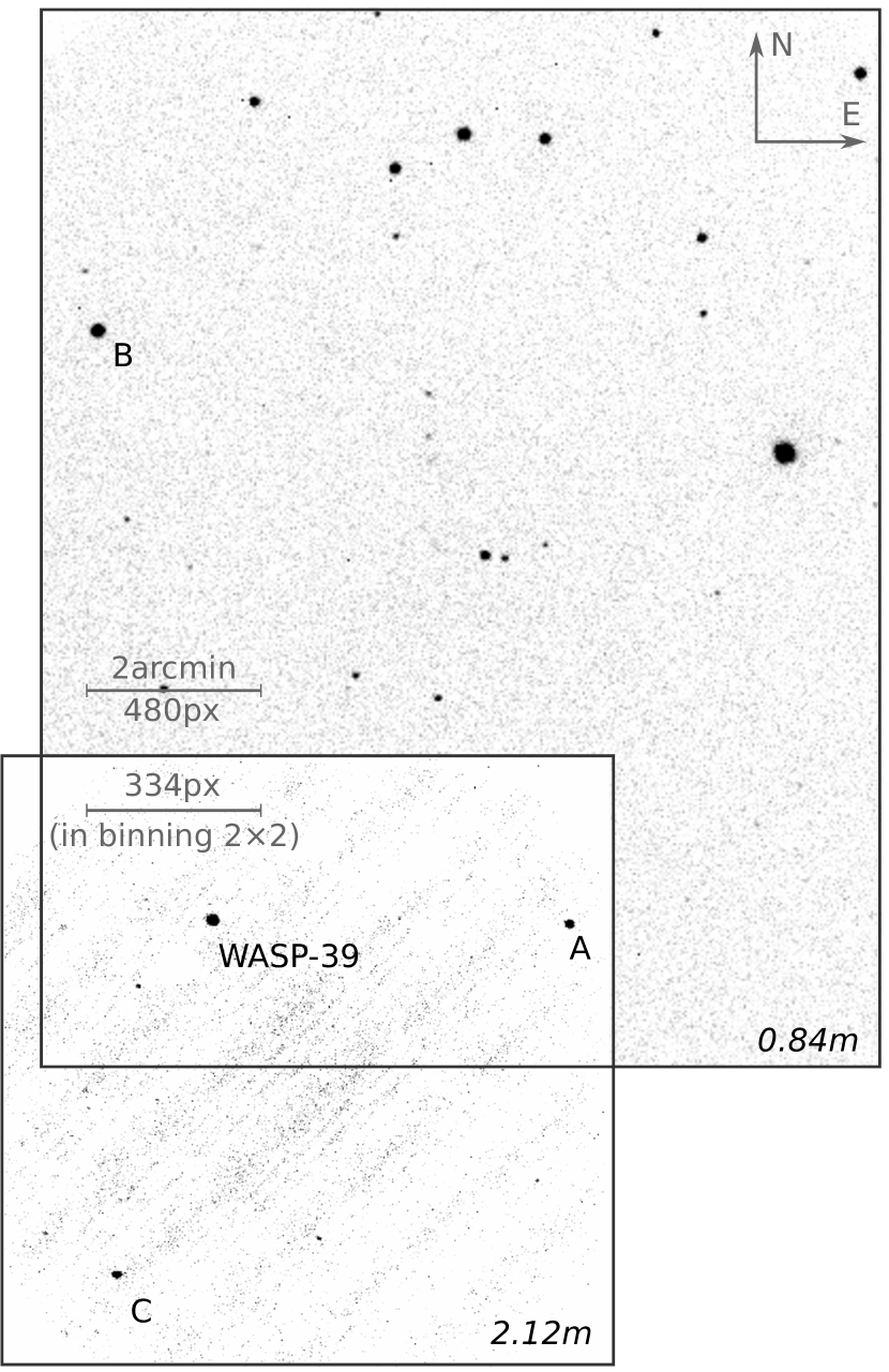
Figure 1: Superposed fields of WASP-39b obtained with the $0.84$ and the $2.12$ telescopes, in two random CCD images, and using an inverse color scale. The target and field stars A, B, and C are also shown. Star A was chosen as a reference for photometry for both the telescopes.

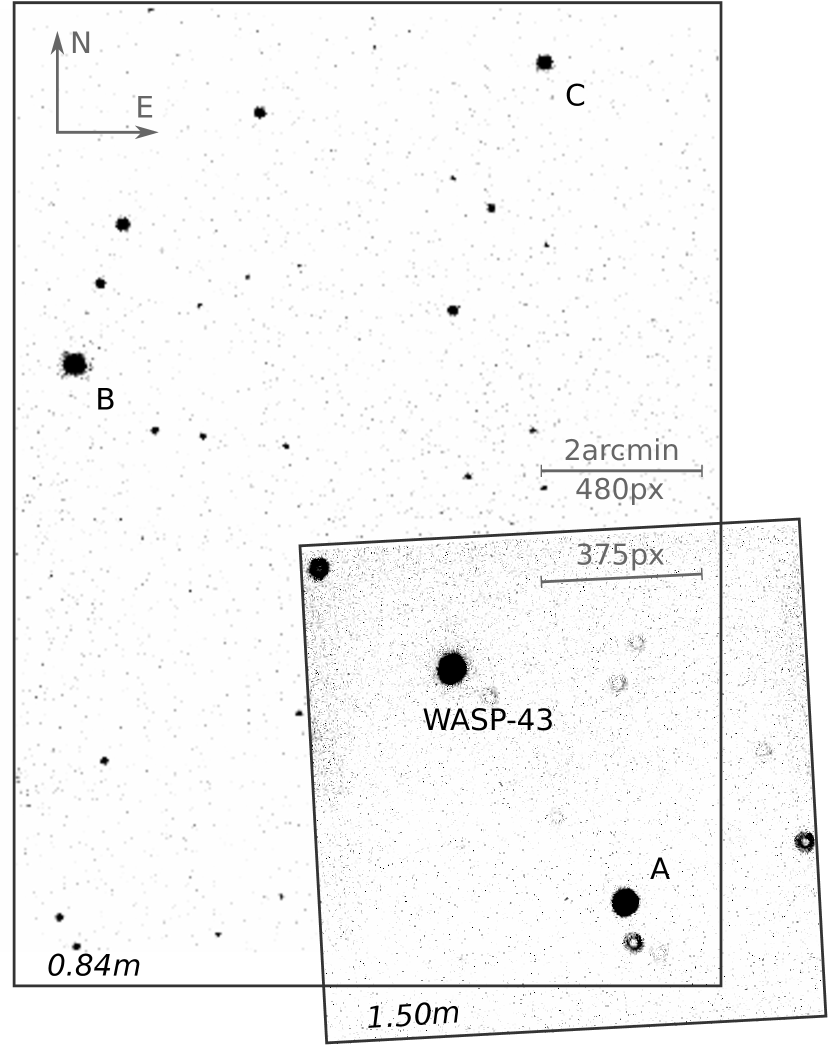
Figure 2: Superposed fields of WASP-43b as obtained with the $0.84$ and the $1.50$ telescopes, in two random CCD images, and using an inverse color scale. The defocusing is particularly appreciable in the $1.50$ telescope images. The target field stars A, B, and C are also shown. Star A was chosen as a reference for photometry for both the telescopes.

Observations were also obtained with the robotic $1.50$ telescope and its multi-channel imager RATIR (Rapchun et al. 2011; Watson et al. 2012; Butler et al. 2012; Farah et al. 2012). This instrument, designed for Gamma Ray Burst observations and follow-up, is equipped with three dichroics to transmit the light to four detectors named C0, C1, C2, and C3, equipped with optical and infrared filters.

The CCDs work in $2\times 2$ binning mode by default. In this paper we present observations carried out using the Gunn-$i$ only, corresponding to the C1 detector which provides a $5.6\arcmin\times 5.6\arcmin$ field of view.

Taking advantage from free observing time during maintenance operations, we had the possibility to use the $2.12$ telescope, improved with active optics on the primary mirror, which is normally dedicated to spectroscopy. We used this telescope in direct-imaging mode. The observation presented in this paper was carried out using the $U$ filter on the Marconi CCD providing a $6.2\arcmin\times 6.2\arcmin$ field of view.

Additional details about telescopes and detectors are listed in Table 1, while Table 2 shows the log of the observations.

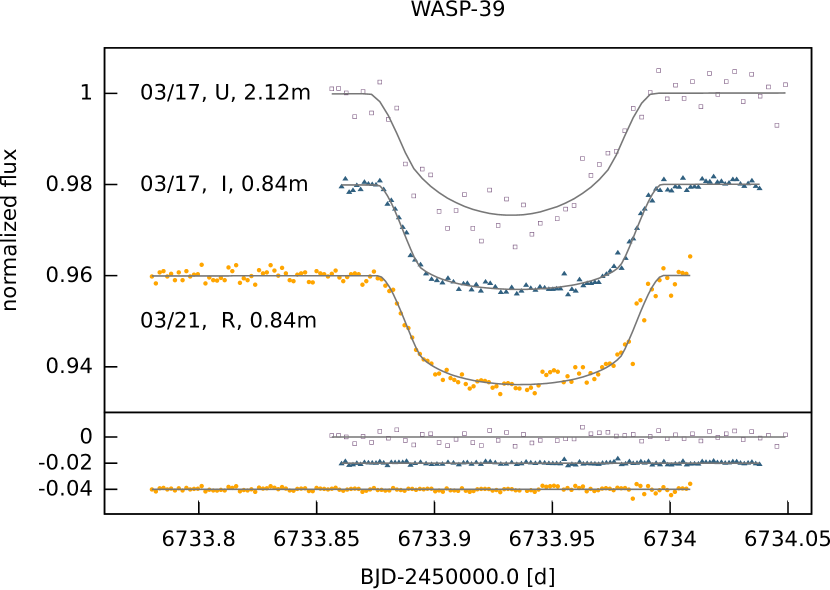
Figure 3: Light curves of WASP-39b obtained with the $0.84$ telescope in $R$ and $I$ bands and with the $2.12$ telescope in the $U$ band. For displaying purposes, the light curves were reported to the time of the last observation (2014-03-21), and an arbitrarily shift is applied. The fit of the light curves (solid lines) is also shown, as well as the residuals in the lower box.

2.1 WASP-39b

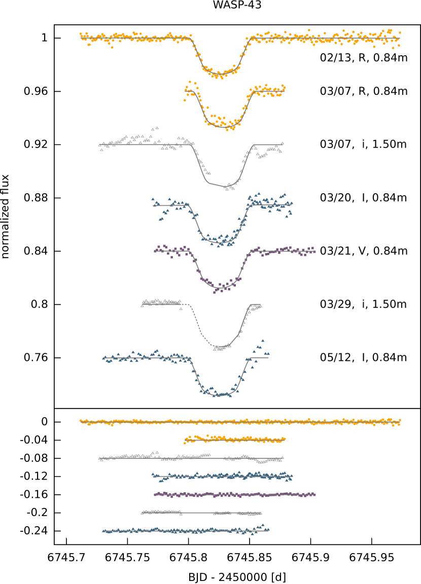
Figure 4: Light curves of WASP-43b obtained with the $0.84$ telescope in $VRI$ bands and with the $1.50$ telescope in the Gunn-$i$ band, reported to the time of the observation of 2014-03-29, and arbitrarily shifted. The fit and the residuals are also shown. The dashed line represent an interpolation of the model.

We performed three observations of WASP-39b, covering two subsequent transits. Its parent star is a G-type dwarf with a reported magnitude of $V=12.1$ (Faedi et al. 2011).

For the transit of 2014-03-17 we had simultaneous access to the $0.84$ and to the $2.12$ telescopes. Fig. 1 shows the target and its nearby stars as seen in the fields of the two telescopes, some of which (A, B and C) were tested as comparison stars, as seen by the fields of the two telescopes. We observed in the $I$ band with the smaller telescope, obtaining 103 frames with exposure times of $120$ and $180$, and in the $U$ band with the larger one, in order to take advantage from its sensitivity, obtaining 57 frames with exposure times of $240$ and $300$. As the object was particularly faint in this filter, we decided to use a $2\times 2$ binning and a small defocus.

The transit of 2014-03-21 was observed with the $0.84$ telescope only. We obtained 142 frames in the $R$ band with an exposure time of $120$, slightly defocusing the telescope to avoid saturation.

The night conditions during all observations suffered from very thin high haze and a nearly-full Moon, with a seeing of about $3$–$4\arcsec$. Depending on the instrument, the band, and seeing conditions, different defocusing levels were used. Moreover, rapid changes in the atmospheric conditions required a variation of the exposure time in order to avoid saturation.

2.2 WASP-43b

Due to its short period with respect to WASP-39b, we had the opportunity to carry out more observations of WASP-43b. We obtained a total of seven transits spanning six nights. Fig. 2 shows two fields containing the target and nearby stars as seen with the $0.84$ and $1.50$ telescopes.

Four transits were observed with the $0.84$ telescope only: on 2014-02-13, 2014-03-20, 2014-03-21, 2014-05-12 in the $R$, $I$, $V$, and again $I$ filters, respectively, with exposure times spanning from $60$ to $120$.

Another transit was obtained with the $1.50$ telescope only (2014-03-29), strongly defocused, in the Gunn-$i$ filter, and with a $90$ exposure time. This transit was unfortunately affected by clouds from the first contact until almost the mid time.

Finally, we observed with both the $0.84$ and $1.50$ telescopes on 2014-03-07, using the $R$ and Gunn-$i$ filters respectively, and with exposure times of $60$ and $140$.

All observations were taken in condition of a nearly-full moon.

3 Data reduction

CCD images of both transits were debiased and flat-fielded using standard IRAF procedures from the ccdproc package. Master bias and master sky flat fields were obtained from images taken at the beginning and at the end of each observing night. Cosmic rays were also removed using the method implemented by the lakos package van Dokkum (2001), then images were aligned using the imalign IRAF procedure.

We decided to use different aperture photometry routines to obtain the light curves: a custom IRAF routine and the defot routine (Southworth et al. 2010) written in the IDL language, that we modified to work with the FITS headers generated by the SPM-OAN telescopes. We found that the results of these two pipelines are in good agreement. In the case of images with a small amount of defocus, it was possible to calculate the Full Width Half Maximum (FWHM) of the Point Spread Function by fitting an elliptical Gaussian. We used this information to dynamically adapt the aperture radius to a value of 2.5 times the calculated FWHM. We found that this technique increases the quality of the photometry with respect to the fixed-radius aperture. In the case of images with a consistent defocus, several fixed apertures were tested in order to find the optimal value.

Several field stars were tested in order to find a reference star to perform differential photometry, and a non-saturated star with a color index and magnitude values as close as possible to those of the target star was chosen. The chosen reference stars for WASP-39b and WASP-43b are labeled as “A” in Fig. 1 and Fig. 2, respectively.

We then used the target and the reference star to produce differential light curves.

The resulting light curves may present some residual trends, which were removed with a first-order airmass correction described by Ramón-Fox & Sada (2013).

The timestamps of the light curve were converted to the Dynamical Time-based system ($BJD_{\rm TDB}$, here therefore $BJD$) using the transformation given by Eastman et al. (2010).

We used the aperture photometry technique presented above for both WASP-39b, whose three final light curves are presented in Fig. 3, and WASP-43b, whose seven final light curves are shown in Fig. 4.

3.1 Fit

Table 3: Fit results of the physical and orbital parameters of WASP-39b and WASP-43b obtained with TAP. The fit of the period and the period variation are described in Sect. 4.

Parameter	Filter	WASP-39	WASP-43
$i$ []		$87.78\pm 0.43$	$81.92\pm 0.54$
$a/R_{*}$		$11.32\pm 0.42$	$4.82\pm 0.11$
	$U$	$0.1462\pm 0.0116$
	$V$		$0.1615\pm 0.0041$
$R_{p}/R_{*}$	$R$	$0.1424\pm 0.0023$	$0.1599\pm 0.0025$
	$I$	$0.1424\pm 0.0023$	$0.1653\pm 0.0054$
	$i$		$0.1738\pm 0.0033$
$P$ [d]		4.055259	0.81347437
$e$		0	0
$\omega$ []		0	0
	$U$	0.950
	$V$		0.750
$l_{1}$	$R$	0.425	0.599
	$I$	0.335	0.451
	$i$		0.485
	$U$	-0.086
	$V$		0.040
$l_{2}$	$R$	0.246	0.137
	$I$	0.250	0.193
	$i$		0.183

The light curves were fitted using the IDL software Transit Analysis Package (TAP) implemented by Gazak et al. (2011), which uses a Markov Chain Monte Carlo (MCMC) method to find the best fit parameters for the Mandel & Agol (2002) model.

This code allows to fit multiple light curves simultaneously, which is particularly useful for fixing parameters such as the orbital inclination $i$ and the scaled semi-major axis $a/R_{*}$ to the same values for a group of curves, and thus obtain a global fit for these quantities.

Other parameters, such as the mid-transit time $T_{mid}$ and the scaled planetary radius $R_{p}/R_{*}$ are allowed to be fitted individually for each curve. This technique allows to fit the same orbital model to a group of light curves of the same object obtained in different bands, and to find potential planetary radius differences as a function of the wavelength.

All light curves of each system were fitted simultaneously. We used a set of fixed values in the MCMC analysis for several parameters: the Period $P$, taken from Faedi et al. (2011) for WASP-39b and from Chen et al. (2014) for WASP-43b; the eccentricity $e$ and the argument of periastron $\omega$, both set $=0$. TAP allows the use of linear and quadratic models for the stellar limb darkening. A quadratic model is assumed in this analysis, and the two terms $l_{1}$ (linear) and $l_{2}$ (quadratic) are fixed in the MCMC analysis to the values corresponding to the filter used for each light curve. The values were obtained from the exofast (Eastman et al. 2012, 2013) online tool, which are interpolated from stellar atmosphere models of Claret & Bloemen (2011).

We then fitted for each system: the orbital inclination $i$, the scaled semi-major axis $a/R_{*}$, and a value of the scaled radius $R_{p}/R_{*}$ for each one of the used filters. TAP was initialized with the most recent parameters reported in Faedi et al. (2011) for WASP-39b and Chen et al. (2014) for WASP-43b.

The mid-transit time $T_{mid}$ for each light curve was also fitted (in the case of multiple light curves of the same object obtained on the same night using different telescopes, the same $T_{mid}$ was fitted for both the light curves). For the MCMC analysis, the $T_{mid}$ is initialized with a value estimated by TAP from the input light curve.

The best-fit models and corresponding residuals are shown in Figs. 3 and 4, and the values of the parameters are shown in Table 3.

4 Period and period variation

Using the fitted values for the mid-transit time $T_{mid}$, we retrieved the period $P$ of WASP-39b and WASP-43b by fitting the following linear law:

$$T_{mid}=T_{0}+NP,$$ (1)

where $T_{0}$ is the initial epoch and $N$ is the number of periods since $T_{0}$. $T_{0}$ and $P$ are best-fit parameters.

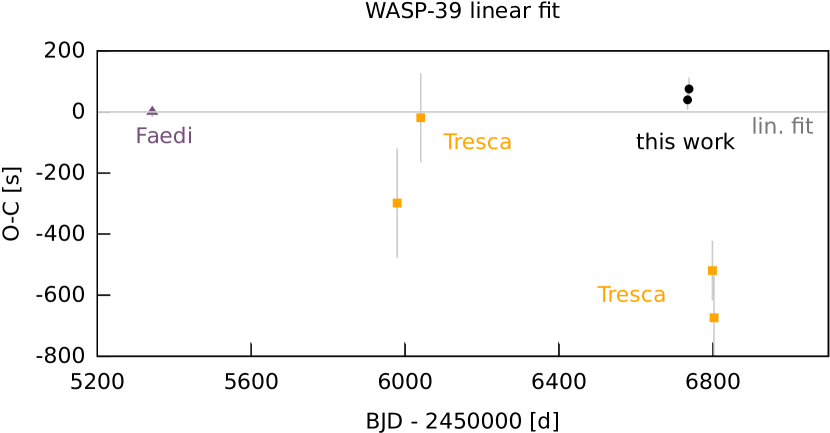
Figure 5: Observed $-$ calculated $T_{mid}$ and linear fit of the WASP-39b period, including data from Faedi et al. (2011), from the ETD-TRESCA database, and from our observations.

Further analysis of the ephemerids was carried out in order to investigate a long-term variation of the period with respect to the time. A constant decrease of the period for close-orbiting planets may be indicative of processes that remove orbital energy such as tidal dissipation (Adams et al. 2010b, a; Sasselov 2003; Levrard et al. 2009). A simple model assuming a constant variation of the period is given by the following quadratic equation

$$T_{mid}=T_{0}+NP+\delta PN(N-1)/2$$ (2)

proposed by Adams et al. (2010a), where $\delta P=P\dot{P}$.

For the present analysis, a Levenberg-Marquardt least-squares fitting algorithm implemented in the code of Markwardt (2009) was initially used to find the best-fit parameters of Eqs. 1 and 2. However, this algorithm can be trapped in a local minimum of $\chi^{2}$. For this reason, a Monte Carlo code was set-up to search for the $\chi^{2}$ minimum and sample the parameter space. Both approaches were tested on the OGLE-TR-113b (catalog ) data provided by Adams et al. (2010b), finding good agreement with their results.

We find that both approaches are consistent and give similar best-fit values. Comforted by these results, we decided to apply this method to our data, and we describe the results in the following subsections.

4.1 WASP-39b

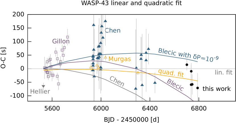
Figure 6: Observed $-$ calculated $T_{mid}$, linear and quadratic fit of the WASP-43b period including data from Hellier et al. (2011); Gillon et al. (2012); Chen et al. (2014); Murgas et al. (2014), and from our observations. See Sect. 4.2 for curve details.

Concerning WASP-39b, the $T_{mid}$ reported by Faedi et al. (2011) and the one calculated from our observations are fitted using Eq. 1. This gives a

• $T_{0}=2455342.9687998\pm 0.0001999$ (BJD),

• $P=4.0552989\pm 9.963\times 10^{-7}$ days. This fit has a

• $\chi^{2}=0.541$,

where $\chi^{2}$ stands for the “reduced $\chi^{2}$”, i.e. $\chi^{2}/D_{f}$, where $D_{f}$ are the degrees of freedom (number of data $-$ number of parameters).

However, due to the significantly small number of observations, we decided to increase the number of transits considered in our analysis by introducing additional data from the Exoplanet Transit Database (ETD) webpage (Poddaný et al. 2010), in order to improve the robustness of our results. We selected a total of three light curves. According to this database, the timings of the light curves are reported in HJD. They were transformed to BJD using the software provided by Eastman et al. (2010). We used TAP to obtain only $T_{mid}$ for these light curves by running the MCMC analysis with all other parameters to be fixed to the values provided by Faedi et al. (2011). By adding these new data to previous ones, we obtain a total of 7 observations. The linear fit of Eq. 1 was repeated with these additional transits, and the following results were obtained:

• $T_{0}=2455342.9695727\pm 0.000199$ (BJD),

• $P=4.0552947\pm 9.651\times 10^{-7}$ days, and a

• $\chi^{2}=11.82$,

indicating a period larger than that reported by Faedi et al. (2011). The residuals for this fit are shown in Fig. 5. As the last two Tresca points show large differences with respect to the fit, we tested the fit process without their contribution, obtaining the following results:

• $T_{0}=2455342.9695554\pm 0.0001994$ (BJD),

• $P=4.0552965\pm 9.956\times 10^{-7}$ days, and a

• $\chi^{2}=1.299$,

and in this case too we report a larger period with respect to Faedi et al. (2011) results. In both cases the results are consistent, but we suggest to improve their robustness with additional observations.

An attempt to fit Eq. 2 was made, but the small amount of data do not allow a reasonable result for the fit. More data are needed as well as precise timings, in order to assess if there is a long-term constant variation of the period, or to detect the presence of other transit timing variations.

4.2 WASP-43b

A sufficient amount of WASP-43b transit timings is available in the literature spanning several years of observations (Hellier et al. 2011; Gillon et al. 2012; Chen et al. 2014; Murgas et al. 2014).

Some previous studies of possible long-term variations have been carried out by Chen et al. (2014) and Murgas et al. (2014), suggesting that the period of WASP-43b is slowly decreasing with time. In this work, we repeat the analysis combining our data with the timings available in the literature. A best-fit model was obtained using the Marquardt-Levenberg algorithm previously described. For the linear fit, best-fit values are

• $T_{0}=2455528.86839966\pm 0.000036904078$ (BJD), and

• $P=0.81347409\pm 7.3\times 10^{-8}$ days, giving a

• $\chi^{2}=3.784$.

For the quadratic fit, best fit values are

• $T_{0}=2455528.86848347\pm 0.0000369043$ (BJD),

• $P=0.81347374\pm 7.285\times 10^{-8}$ days, and a

• $\delta P=6.7\pm 6.9\times 10^{-10}$, corresponding to

• $\dot{P}=0.03\pm 0.03/\rm{year}$ . This gives a

• $\chi^{2}=3.819$.

The small difference in $\chi^{2}$ between the linear and quadratic fits shows that, statistically, there is no significant improvement by using the latter, as shown in Fig. 6.

Using the values provided by Blecic et al. (2014), we obtain

• $P=0.81347530\pm 3.9\times 10^{-7}$ days, and

• $\dot{P}=-0.095\pm 0.036/\rm{year}$, giving a

• $\chi^{2}=21.25$.

The parameters reported by Chen et al. (2014) are

• $P=0.81347399\pm 2.2\times 10^{-7}$ days, and we have

• $\dot{P}=-0.09\pm 0.04/\rm{year}$, giving a

• $\chi^{2}=18.26$.

The fit was also tested with the Monte Carlo approach which find a a minimum $\chi^{2}$ corresponding to $P=0.81347382$ and $\dot{P}=0.02/\rm{year}$, with a $\chi^{2}=4.046$. This analysis showed that the $\chi^{2}$ minimum is very close to a value of $\dot{P}=0$.

These fits are visualized in Fig. 6. The model of Blecic et al. (2014) fits most of the points reasonably well, except for those corresponding to our observations. The model of Chen et al. (2014) shows more deviations with respect to recent observations. For comparison, we also plot a third model using the same period reported by Blecic et al. (2014) but with a

• $\delta P=-1.0\times 10^{-9}$, which is in the order of magnitude of previously reported values, giving a

• $\chi^{2}=46.96$.

This corresponds to the same orbital period of Blecic et al. (2014) but with a smaller value of $\dot{P}=-0.038/\rm{year}$. It can be seen that it fits reasonably points from earlier observations.

However, a detailed analysis of Transit Time Variations has not been considered in this work, which could explain some of the observed variations (Chen et al. 2014).

The present analysis then confirms the results of Chen et al. (2014), also showing that a quadratic model does not improve significantly the fit of the transit timings for WASP-43b.

5 Results and discussion

We report for the first time a light curve of WASP-39b in the $U$ band obtained with the $2.12$ telescope at SPM-OAN. Observations in this band are important to study the presence of high-hazes in the atmosphere, as Rayleigh scattering becomes important at smaller wavelengths, which can produce larger observed radii in this band (Southworth et al. 2012a; Copperwheat et al. 2013). The resulting light curve is shown in Fig. 3. Although there is more dispersion in the data compared to the $I$ and $R$ bands, a depth flux of approximately $3\%$ is observed. The best-fit values obtained in the previous section give a relative radius of $R_{p}/R_{*}=0.1462\pm 0.0116$.

No significant variations of the planetary radius between the $U$, $R$, and $I$ bands is found. It is also noted that the $U$ and $I$ band light curves were obtained in the same night, and no evident asymmetries are observed that could suggest the presence of tails or other features around the planet. Additional observations in the $U$ band can help to reduce the uncertainty for this highly inflated extrasolar planet.

The analysis of the ephemerids in the previous section gives a period for WASP-39b approximately $3.084\pm 0.774$ larger than that of Faedi et al. (2011).

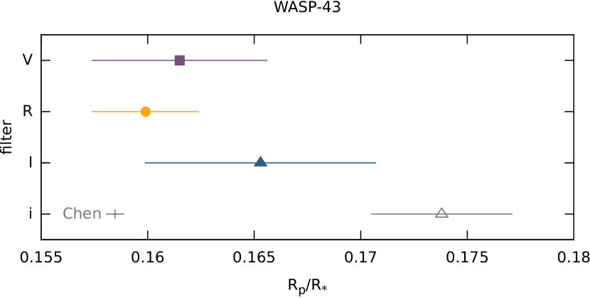
Figure 7: WASP-43b planet radius in the observing filters (see Table 3). The value reported by Chen et al. (2014) in the $i$ filter is also shown.

WASP-43b shows a slight dependence of the $R_{p}/R_{*}$ as a function of the used filter (see Fig. 7), which should be investigated with additional observations. In particular, we find for filter $i$ a value higher by $0.01637\pm 0.00371$ with respect to the value reported by Chen et al. (2014) in the same filter. ($0.1738\pm 0.0033$ against $0.15847\pm 0.00041$). Although, as our two $i$ filter curves are not complete and show signatures of red noise, we suggest to carry on more observations to confirm the significancy of this result.

Nevertheless, we find a tendency for the $R_{p}/R_{*}$ similar to that of Chen et al. (2014) in the sense that the planetary radius is significantly higher at the $i$ band with respect to the value in other bands. The semi-major axis is slightly smaller, but comparable to the value obtained by Gillon et al. (2012) and Chen et al. (2014).

The analysis of the ephemerids gives a period consistent with previous results, and we confirm that there is no improvement while using a quadratic model for fitting the ephemerids. Further analysis and observations would be required to ascertain if a constant period variation exists for WASP-43b. Given the proximity of this planet to its host star, this is particularly relevant to explore potential mechanisms that remove orbital energy such as tidal dissipation.

The present work is part of an ongoing survey started in 2014. A total of 23 extrasolar planets were observed mainly with the $0.84$ and the $1.50$ telescopes giving a total of 40 good quality light curves in several filters. Upgrades in the instrumentation, refinement of the observing technique, and the possibility to benefit from dark and photometric nights will increase the quality of the results in the near future, and will complement other telescope data for multi-site studies and analysis of this class of objects. Moreover, three new $1.30$ telescopes will be completed by 2016 at the San Pedro Mártir observatory, which are part of the TAOS II project (Lehner et al. 2012a; Geary et al. 2012; Lehner et al. 2013).

The characteristics of this survey (Lehner et al. 2012b) allow to set up specific pipelines for the early detection of new extrasolar planets, for example with a binning of the light curves as already tested for TAOS data (Ricci et al. 2014). Also, a project for the installation of a $6.5$ telescope at the San Pedro Mártir observatory has recently reached the phase of preliminary design.

Current and in fieri SPM-OAN telescopes then represent a unique opportunity for the extrasolar planet community to complement the northern hemisphere observatories involved in this research area.

6 Conclusions

Multi-filter exoplanet transit observations of WASP-39b and WASP-43b, carried on for the first time with all three San Pedro Mártir telescopes, have shown the capability of these facilities of $0.84$, $1.50$ and $2.12$ for this kind of investigation. The fit of the two objects shows a scatter of $1.5$–$2.5\mathrm{m}\rm mag$ rms in condition of full or nearly-full Moon. This makes these instruments suitable for future ground-based observing campaigns, in particular for the follow-up of alerts triggered by the upcoming projects currently in development.

The analysis shows most of the parameters to be in good agreement with previous works, in particular for what concerns the first observation WASP-39b in the $U$ filter.

The period for WASP-39b is found to be significantly larger ($>3$) with a $4\sigma$ accuracy with respect to previous works.

The value of the planet/star radius of WASP-43b is larger in the $i$ filter with respect to previous works.

A tendency of a higher planet radius in the $i$ band is obtained, consistent with the tendency reported in recent works. Additional observations of this object are needed to confirm a slight dependence of this parameter on the observing filter.

We suggest to plan additional observations in order to confirm the accuracy of these result with respect to the literature.

References

- Adams et al. (2010a) Adams, E. R., Lopez-Morales, M., Elliot, J. L., Seager, S., & Osip, D. J. 2010a, in Bulletin of the American Astronomical Society, Vol. 42, AAS/Division for Planetary Sciences Meeting Abstracts #42, 1090
- Adams et al. (2010b) Adams, E. R., López-Morales, M., Elliot, J. L., Seager, S., & Osip, D. J. 2010b, ApJ, 721, 1829
- Baglin et al. (2009) Baglin, A., Auvergne, M., Barge, P., et al. 2009, in IAU Symposium, Vol. 253, IAU Symposium, ed. F. Pont, D. Sasselov, & M. J. Holman, 71–81
- Baglin & Catala (2009) Baglin, A., & Catala, C. 2009, in SF2A-2009: Proceedings of the Annual meeting of the French Society of Astronomy and Astrophysics, ed. M. Heydari-Malayeri, C. Reyl’E, & R. Samadi, 27
- Bakos et al. (2007) Bakos, G. Á., Noyes, R. W., Kovács, G., et al. 2007, ApJ, 656, 552
- Baranne et al. (1996) Baranne, A., Queloz, D., Mayor, M., et al. 1996, A&AS, 119, 373
- Batalha et al. (2014) Batalha, N., Kalirai, J. S., Lunine, J. I., & Mandell, A. 2014, in American Astronomical Society Meeting Abstracts, Vol. 223, American Astronomical Society Meeting Abstracts, #325.03
- Blecic et al. (2012) Blecic, J., Harrington, J., Madhusudhan, N., et al. 2012, in AAS/Division for Planetary Sciences Meeting Abstracts, Vol. 44, AAS/Division for Planetary Sciences Meeting Abstracts, #103.07
- Blecic et al. (2014) Blecic, J., Harrington, J., Madhusudhan, N., et al. 2014, ApJ, 781, 116
- Borucki et al. (2010) Borucki, W. J., Koch, D., Basri, G., et al. 2010, Science, 327, 977
- Butler et al. (2012) Butler, N., Klein, C., Fox, O., et al. 2012, in Society of Photo-Optical Instrumentation Engineers (SPIE) Conference Series, Vol. 8446, Society of Photo-Optical Instrumentation Engineers (SPIE) Conference Series
- Chen et al. (2014) Chen, G., van Boekel, R., Wang, H., et al. 2014, A&A, 563, A40
- Clampin (2008) Clampin, M. 2008, Advances in Space Research, 41, 1983
- Claret & Bloemen (2011) Claret, A., & Bloemen, S. 2011, A&A, 529, A75
- Copperwheat et al. (2013) Copperwheat, C. M., Wheatley, P. J., Southworth, J., et al. 2013, MNRAS, 434, 661
- Czesla et al. (2013) Czesla, S., Salz, M., Schneider, P. C., & Schmitt, J. H. M. M. 2013, A&A, 560, A17
- Eastman et al. (2012) Eastman, J., Gaudi, B. S., & Agol, E. 2012, EXOFAST: Fast transit and/or RV fitter for single exoplanet, astrophysics Source Code Library, ascl:1207.001
- Eastman et al. (2013) —. 2013, PASP, 125, 83
- Eastman et al. (2010) Eastman, J., Siverd, R., & Gaudi, B. S. 2010, PASP, 122, 935
- Faedi et al. (2011) Faedi, F., Barros, S. C. C., Anderson, D. R., et al. 2011, A&A, 531, A40
- Farah et al. (2012) Farah, A., González, J. J., Kutyrev, A. S., et al. 2012, in Society of Photo-Optical Instrumentation Engineers (SPIE) Conference Series, Vol. 8446, Society of Photo-Optical Instrumentation Engineers (SPIE) Conference Series
- Gazak et al. (2011) Gazak, J. Z., Johnson, J. A., Tonry, J., et al. 2011, Transit Analysis Package (TAP and autoKep): IDL Graphical User Interfaces for Extrasolar Planet Transit Photometry, astrophysics Source Code Library, ascl:1106.014
- Geary et al. (2012) Geary, J. C., Wang, S.-Y., Lehner, M. J., Jorden, P., & Fryer, M. 2012, in Society of Photo-Optical Instrumentation Engineers (SPIE) Conference Series, Vol. 8446, Society of Photo-Optical Instrumentation Engineers (SPIE) Conference Series
- Gillon et al. (2012) Gillon, M., Triaud, A. H. M. J., Fortney, J. J., et al. 2012, A&A, 542, A4
- Hellier et al. (2011) Hellier, C., Anderson, D. R., Collier Cameron, A., et al. 2011, A&A, 535, L7
- Husnoo et al. (2012) Husnoo, N., Pont, F., Mazeh, T., et al. 2012, MNRAS, 422, 3151
- Kreidberg et al. (2014) Kreidberg, L., Bean, J. L., Désert, J.-M., et al. 2014, ApJ, 793, L27
- Lehner et al. (2013) Lehner, M., Wang, S., Ho, P., et al. 2013, in AAS/Division for Planetary Sciences Meeting Abstracts, Vol. 45, AAS/Division for Planetary Sciences Meeting Abstracts, #414.08
- Lehner et al. (2012a) Lehner, M. J., Wang, S.-Y., Alcock, C. A., et al. 2012a, in Society of Photo-Optical Instrumentation Engineers (SPIE) Conference Series, Vol. 8444, Society of Photo-Optical Instrumentation Engineers (SPIE) Conference Series
- Lehner et al. (2012b) Lehner, M. J., Wang, S., Alcock, C. A., et al. 2012b, in AAS/Division for Planetary Sciences Meeting Abstracts, Vol. 44, AAS/Division for Planetary Sciences Meeting Abstracts, #310.20
- Levrard et al. (2009) Levrard, B., Winisdoerffer, C., & Chabrier, G. 2009, ApJ, 692, L9
- Line et al. (2014) Line, M. R., Knutson, H., Wolf, A. S., & Yung, Y. L. 2014, ApJ, 783, 70
- Mandel & Agol (2002) Mandel, K., & Agol, E. 2002, ApJ, 580, L171
- Markwardt (2009) Markwardt, C. B. 2009, in Astronomical Society of the Pacific Conference Series, Vol. 411, Astronomical Data Analysis Software and Systems XVIII, ed. D. A. Bohlender, D. Durand, & P. Dowler, 251
- Mayor & Queloz (1995) Mayor, M., & Queloz, D. 1995, Nature, 378, 355
- Murgas et al. (2014) Murgas, F., Pallé, E., Zapatero Osorio, M. R., et al. 2014, A&A, 563, A41
- Perruchot et al. (2008) Perruchot, S., Kohler, D., Bouchy, F., et al. 2008, in Society of Photo-Optical Instrumentation Engineers (SPIE) Conference Series, Vol. 7014, Society of Photo-Optical Instrumentation Engineers (SPIE) Conference Series
- Poddaný et al. (2010) Poddaný, S., Brát, L., & Pejcha, O. 2010, New A, 15, 297
- Pollacco et al. (2006) Pollacco, D. L., Skillen, I., Collier Cameron, A., et al. 2006, PASP, 118, 1407
- Queloz et al. (2000) Queloz, D., Mayor, M., Naef, D., et al. 2000, in From Extrasolar Planets to Cosmology: The VLT Opening Symposium, ed. J. Bergeron & A. Renzini, 548
- Ramón-Fox & Sada (2013) Ramón-Fox, F. G., & Sada, P. V. 2013, Rev. Mexicana Astron. Astrofis., 49, 71
- Rapchun et al. (2011) Rapchun, D. A., Alardin, W., Bigelow, B. C., et al. 2011, in Bulletin of the American Astronomical Society, Vol. 43, American Astronomical Society Meeting Abstracts #217, #157.07
- Rauer et al. (2013) Rauer, H., Catala, C., Aerts, C., et al. 2013, ArXiv e-prints, arXiv:1310.0696
- Ricci et al. (2014) Ricci, D., Sprimont, P.-G., Ayala, C., et al. 2014, ArXiv e-prints, arXiv:1408.6189
- Ricker et al. (2010) Ricker, G. R., Latham, D. W., Vanderspek, R. K., et al. 2010, in Bulletin of the American Astronomical Society, Vol. 42, American Astronomical Society Meeting Abstracts #215, #450.06
- Sasselov (2003) Sasselov, D. D. 2003, ApJ, 596, 1327
- Southworth et al. (2012a) Southworth, J., Mancini, L., Maxted, P. F. L., et al. 2012a, MNRAS, 422, 3099
- Southworth et al. (2009a) Southworth, J., Hinse, T. C., Jørgensen, U. G., et al. 2009a, MNRAS, 396, 1023
- Southworth et al. (2009b) Southworth, J., Hinse, T. C., Burgdorf, M. J., et al. 2009b, MNRAS, 399, 287
- Southworth et al. (2010) Southworth, J., Mancini, L., Novati, S. C., et al. 2010, MNRAS, 408, 1680
- Southworth et al. (2012b) Southworth, J., Hinse, T. C., Dominik, M., et al. 2012b, MNRAS, 426, 1338
- Southworth et al. (2013) Southworth, J., Mancini, L., Browne, P., et al. 2013, MNRAS, 434, 1300
- Southworth et al. (2014) Southworth, J., Hinse, T. C., Burgdorf, M., et al. 2014, MNRAS, 444, 776
- van Dokkum (2001) van Dokkum, P. G. 2001, PASP, 113, 1420
- Wang et al. (2013a) Wang, W., van Boekel, R., Madhusudhan, N., et al. 2013a, in Protostars and Planets VI, Heidelberg, July 15-20, 2013. Poster #2G012, 12
- Wang et al. (2013b) Wang, W., van Boekel, R., Madhusudhan, N., et al. 2013b, ApJ, 770, 70
- Watson et al. (2012) Watson, A. M., Richer, M. G., Bloom, J. S., et al. 2012, in Society of Photo-Optical Instrumentation Engineers (SPIE) Conference Series, Vol. 8444, Society of Photo-Optical Instrumentation Engineers (SPIE) Conference Series
- Wolszczan (1994) Wolszczan, A. 1994, Science, 264, 538
- Wolszczan & Frail (1992) Wolszczan, A., & Frail, D. A. 1992, Nature, 355, 145