Intrinsic spin torque without spin-orbit coupling

Abstract

We derive an intrinsic contribution to the non-adiabatic spin torque for non-uniform magnetic textures. It differs from previously considered contributions in several ways and can be the dominant contribution in some models. It does not depend on the change in occupation of the electron states due to the current flow but rather is due to the perturbation of the electronic states when an electric field is applied. Therefore it should be viewed as electric-field-induced rather than current-induced. Unlike previously reported non-adiabatic spin torques, it does not originate from extrinsic relaxation mechanisms nor spin-orbit coupling. This intrinsic non-adiabatic spin torque is related by a chiral connection to the intrinsic spin-orbit torque that has been calculated from the Berry phase for Rashba systems.

I introduction

Electrical manipulation of magnetization is a promising technique for enabling a new generation of magnetoelectronic devices. Spin-transfer torqueBerger84JAP ; Slonczewski96JMMM ; Berger96PRB ; Ralph08JMMM is an efficient way to implement the electrical control of magnetization, as has been demonstrated for various magnetic nanostructures such as spin valves, magnetic tunnel junctions, and magnetic nanowires. In the standard picture of spin-transfer torque, an external electric field generates a spin-polarized electrical current, which in turn gives rise to current-induced spin-transfer torque. In magnetic nanowires with continuously varying magnetic textures, this picture leads to two components of current-induced spin torque, which are known as adiabatic spin torqueBerger84JAP ; Tatara04PRL and non-adiabatic spin torque.Zhang04PRL ; Thiaville05EPL The adiabatic spin torque arises from spin angular momentum conservation when conduction electron spins adiabatically follow the local magnetization direction.

The non-adiabatic spin torque, which is perpendicular to the adiabatic spin torque, arises from a variety of mechanisms and is a crucial factor for efficient electrical manipulation of magnetic textures such as magnetic domain walls and skyrmions. One mechanism for non-adiabatic spin torques occurs only for very short length scale variations in the magnetic texture,Tatara07JPSJ ; Tatara04PRL ; Xiao06PRB when the spins cannot adiabatically follow the magnetization texture. In slowly varying magnetic textures, all previously considered mechanisms for non-adiabatic spin torques derive from either spin relaxationZhang04PRL or spin-orbit couplingGarate09PRB related to magnetic damping.Kambersky07PRB Here, we describe an intrinsic contribution to the non-adiabatic spin torque that arises in the slowly varying limit from an effective spin-orbit coupling due to the magnetic texture. It is distinguished from other contributions in that it is electric-field-induced rather than current-induced.

The distinction we are trying to draw between electric-field-induced and current-induced torques is potentially confusing because current and electric field are proportional to each other. In linear response, either torque can be written as proportional to either the current or the field. The difference we would like to draw is in how the leading order constants of proportionality depend on the electron momentum-relaxation lifetime. By current-induced torque, we mean one that is proportional to the current with a coefficient that is independent of the lifetime and is proportional to the electric field with a coefficient that is proportional to the lifetime (or conductivity). By electric-field induced effect, we mean one that is proportional to the electric field with a coefficient that is independent of the lifetime and is proportional to the current with a coefficient that is inversely proportional to the lifetime.

Electric-field-induced spin-transfer torques differ from current-induced spin-transfer torques in that they do not originate from the electron occupation change giving rise to current flow. Instead, they originate from the perturbation of the electronic states by an external electric field. In general, electric-field-induced effects depend on the modification of the electron states summed over the whole Fermi sea, much as densities involve the sum over all occupied states, while current-induced effects depend on properties only at the Fermi surface, much as electrical currents do. Examples of electric-field-induced effects include voltage-induced magnetic anisotropy changes,Wang12NM ; Shiota12NM the intrinsic spin Hall effect,Tanaka08PRB and the intrinsic spin-orbit torque.Kurebayashi14NN Electric-field-induced torques are promising for significantly enhancing electrical manipulation efficiencies.Shiota12NM ; Wang12NM ; Kurebayashi14NN ; Liu12Science Unfortunately their mechanisms are less well understood than current-induced spin-transfer torques.

In this paper, we examine electron transport through continuously varying magnetic textures and demonstrate the existence of an electric-field-induced spin torque. The result is intrinsic in the sense that it is independent of impurity scattering rates. For a free electron dispersion, we find that this electric-field-induced torque has the same form as the non-adiabatic spin torque but does not originate from extrinsic relaxation mechanisms, spin-orbit coupling, nor rapidly varying textures. Moreover, we demonstrate that it is significantly larger than other contributions to the non-adiabatic spin torque in some models, making it potentially important for optimizing the manipulation of magnetic structures such as magnetic domain walls and Skyrmions.

The intrinsic non-adiabatic spin torque that we report here is closely related to the intrinsic spin-orbit torqueKurebayashi14NN calculated from a Berry phase. Previously, we reportedKim13PRL that spin-orbit coupling generates chirality in magnetic properties and that many properties of a system acquire chiral counterparts upon the introduction of spin-orbit coupling. We demonstrate below that the intrinsic spin-orbit torque is the chiral counterpart of the intrinsic non-adiabatic spin torque that we report here. This connection indicates the common origin of the two, which can be computed through a variety of techniques including a Berry phase as done earlierKurebayashi14NN or perturbation theory like we do here. This intrinsic spin-orbit torque is also electric-field-induced in the terminology we use in this paper.

We present our result with a free electron model with exchange splitting for illustration, but the result can be easily generalized for arbitrary dispersions. As is the case for the spin Hall effect in the closely related system with Rashba spin-orbit coupling,Sinova04PRL ; Inoue04PRB the intrinsic non-adiabatic spin torque is exactly canceled by vertex corrections due to spin-independent scattering.Tatara07JPSJ However, we demonstrate that such exact cancellation only occurs for non-magnetic scatterersInoue06PRL and this particular free-electron model.

This paper is organized as follows. In Sec. II, we present our model and summarize the central results. In Sec. III, we provide detailed derivation and some remarks for more motivated readers. In Sec. IV, we discuss implications of our result, as an intrinsic origin of non-adiabatic spin-transfer torque. In addition, we discuss the relationship of these results through Onsager reciprocity and a chiral connection with previously developed results. We summarize the paper in Sec. V.

II Results

In this section we illustrate the results of our calculation by applying it to a model based on the free electron dispersion and ignore the vertex corrections. This model allows us to summarize our key results and provide a more intuitive description before presenting a formal derivation. A derivation and discussion of more general models are given in Sec. III.

We consider the Hamiltonian

$$H=\frac{{\bm{\mathrm{p}}}^{2}}{2m_{\rm e}}+J{\bm{\mathrm{\sigma}}}\cdot{\bm{\mathrm{m}}}({\bm{\mathrm{r}}},t),$$ (1)

where ${\bm{\mathrm{p}}}$ is the electron momentum operator, $m_{\rm e}$ is the effective electron mass, ${\bm{\mathrm{\sigma}}}$ is the spin Pauli matrix, ${\bm{\mathrm{m}}}$ is the direction of local magnetization, and $J$ is the exchange energy. In Sec. III, we show that in the slowly varying limit, the system can be described by the locally defined eigenstates which are denoted by $|{\bm{\mathrm{k}}},\pm\rangle_{(0)}$. Here ${\bm{\mathrm{k}}}$ corresponds to the electron momentum and $\pm$ is for minority and majority states. The subscript $(0)$ refers to the eigenstates unperturbed by an electric field. The eigenstates have spins aligned with the magnetization but with small deviations as discussed in Refs. Xiao06PRB, and Aharonov92PRL, and illustrated in Fig. 1(a). The local spin expectation value for the unperturbed eigenstates is

$${\bm{\mathrm{\sigma}}}_{{\bm{\mathrm{k}}},\pm}^{(0)}=\pm{\bm{\mathrm{m}}}\mp\frac{\hbar}{2J}{\bm{\mathrm{m}}}\times({\bm{\mathrm{v}}}_{{\bm{\mathrm{k}}}}\cdot\nabla){\bm{\mathrm{m}}},$$ (2)

where ${\bm{\mathrm{v}}}_{{\bm{\mathrm{k}}}}=\hbar{\bm{\mathrm{k}}}/m_{\rm e}$ is the velocity of the $|{\bm{\mathrm{k}}},\pm\rangle_{(0)}$ state. In equilibrium, the deviations cancel on summing up over all occupied states. However with non-equilibrium electron distributions, they give rise to the current-induced adiabatic spin torque. If an electron relaxation mechanism is present, it relaxes the net deviations, giving the current-induced non-adiabatic spin torque.Zhang04PRL

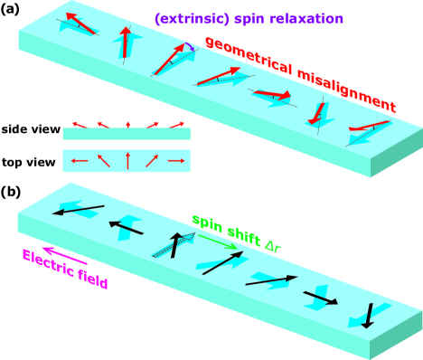
Figure 1: (color online) Illustration of electron spin eigenstates in a spin spiral. (a) The conduction electron spin profile when ${\bm{\mathrm{m}}}$ forms an in-plane spiral (blue thick arrows) in a magnetic nanowire. When the electric field is absent, electron spins (red arrows) have a small out-of-plane component $(\hbar/2J){\bm{\mathrm{m}}}\times({\bm{\mathrm{v}}}_{{\bm{\mathrm{k}}}}\cdot\nabla){\bm{\mathrm{m}}}$ in addition to the local magnetization direction [Eq. (2)]. In equilibrium, the out-of-plane deviation from electrons with momentum ${\bm{\mathrm{k}}}$ and $-{\bm{\mathrm{k}}}$ exactly cancels each other (see Appendix. A or Refs. Aharonov92PRL, ; Xiao06PRB, ). However, an electric field changes the occupations (electrical current) and removes the exact cancellation. The surviving part gives an in-plane spin torque, the adiabatic spin torque. Extrinsic relaxation (purple arrow) of the out-of-plane spin deviation gives an out-of-plane spin torque, the current-induced (or extrinsic) non-adiabatic spin torque. (b) When an electric field is applied, it not only changes the occupation of the electron states but also perturbs the eigenstates giving an additional contribution to spin deviation in the plane (black arrows) by the spin shift [Eq. (3)] (green arrow). This deviation gives rise to an out-of-plane torque, the electric-field-induced (or intrinsic) non-adiabatic spin torque. This in-plane deviation does not cancel for electrons with momentum ${\bm{\mathrm{k}}}$ and $-{\bm{\mathrm{k}}}$. In this figure $\alpha_{{\bm{\mathrm{k}}}}$ and $\Delta{\bm{\mathrm{r}}}$ are exaggerated for clarity.

When an electric field ${\bf E}$ is applied, it perturbs the eigenstates and generates an additional deviation in the spin direction. With the perturbed eigenstates, ${\bm{\mathrm{\sigma}}}_{{\bm{\mathrm{k}}},\pm}={\bm{\mathrm{\sigma}}}_{{\bm{\mathrm{k}}},\pm}^{(0)}+\Delta{\bm{\mathrm{\sigma}}}_{{\bm{\mathrm{k}}},\pm}$ where

$$\Delta{\bm{\mathrm{\sigma}}}_{{\bm{\mathrm{k}}},\pm}=\pm\frac{\hbar^{2}e}{4m_{\rm e}J^{2}}({\bm{\mathrm{E}}}\cdot\nabla){\bm{\mathrm{m}}}.$$ (3)

Here $e>0$ is the electron charge. We demonstrate below that this deviation in the spin direction gives an intrinsic contribution to the non-adiabatic spin torque. Equation (3) is electric-field-induced and is a main result of this paper. This simple picture for the origin of the torque is essentially the same as that givenKurebayashi14NN for the intrinsic spin-orbit torque, which is also electric-field-induced, but differs from that givenGorini08PRB for the current-induced spin polarization, which is a current-induced effect, based on its dependence on the momentum relaxation time. The perturbation due to the electric field here has a characteristic length $\Delta{\bm{\mathrm{r}}}=\hbar^{2}e{\bm{\mathrm{E}}}/4m_{\rm e}J^{2}$. In Fig. 1(b), we show that one way to understand Eq. (3) is to imagine that the electric field shifts the spins spatially by an amount $\Delta{\bm{\mathrm{r}}}$ as in

$${\bm{\mathrm{\sigma}}}_{{\bm{\mathrm{k}}},\pm}[{\bm{\mathrm{m}}}({\bm{\mathrm{r}}},t)]={\bm{\mathrm{\sigma}}}_{{\bm{\mathrm{k}}},\pm}^{(0)}\left[{\bm{\mathrm{m}}}\left({\bm{\mathrm{r}}}+\Delta{\bm{\mathrm{r}}},t\right)\right].$$ (4)

Expanding the functional on the right hand side to lowest order in ${\bm{\mathrm{E}}}$ gives Eq. (2) and Eq. (3).

The equation of motion for the magnetization is given by the Landau-Lifshitz-Gilbert equation including spin torque contributions,

$$\partial_{t}{\bm{\mathrm{m}}}=-\gamma{\bm{\mathrm{m}}}\times{\bm{\mathrm{H}}}_{\rm eff}+\alpha{\bm{\mathrm{m}}}\times\partial_{t}{\bm{\mathrm{m}}}+{\bm{\mathrm{T}}},$$ (5)

where ${\bm{\mathrm{H}}}_{\rm eff}$ is the effective magnetic field and $\alpha$ is the Gilbert damping parameter. The spin torque ${\bm{\mathrm{T}}}$ is calculated from ${\bm{\mathrm{T}}}=(J\gamma/M_{\rm s})\sum_{{\bm{\mathrm{k}}},s}{\bm{\mathrm{m}}}\times{\bm{\mathrm{\sigma}}}_{{\bm{\mathrm{k}}},s}f_{{\bm{\mathrm{k}}},s}$, where $\gamma$ is the gyromagnetic ratio, $M_{\rm s}$ is the saturation magnetization, and $f_{{\bm{\mathrm{k}}},s}$ is the electron distribution function. After some algebra, Eqs. (2) and (3) lead to

$$\frac{\partial{\bm{\mathrm{m}}}}{\partial t} =-\gamma{\bm{\mathrm{m}}}\times{\bm{\mathrm{H}}}_{\rm eff}+\alpha{\bm{\mathrm{m}}}\times\partial_{t}{\bm{\mathrm{m}}}+\frac{\mu_{\rm B}}{eM_{\rm s}}({\bm{\mathrm{j}}}_{\rm s}\cdot\nabla){\bm{\mathrm{m}}}$$

$$\quad-\frac{\beta\mu_{\rm B}}{eM_{\rm s}}{\bm{\mathrm{m}}}\times({\bm{\mathrm{j}}}_{\rm s}\cdot\nabla){\bm{\mathrm{m}}}-\frac{n_{\rm s}\mu_{\rm B}\hbar e}{2m_{\rm e}JM_{\rm s}}{\bm{\mathrm{m}}}\times({\bm{\mathrm{E}}}\cdot\nabla){\bm{\mathrm{m}}},$$ (6)

where $\mu_{\rm B}$ is the Bohr magneton, ${\bm{\mathrm{j}}}_{\rm s}=e\sum_{{\bm{\mathrm{k}}},s}s{\bm{\mathrm{v}}}_{{\bm{\mathrm{k}}}}f_{{\bm{\mathrm{k}}},s}$ is the spin-polarized electrical current density, $n_{\rm s}=-\sum_{{\bm{\mathrm{k}}},s}sf_{{\bm{\mathrm{k}}},s}$ is the spin-polarized density,comment:sign convention and $\beta$ is the non-adiabaticity parameter.Thiaville05EPL ; Zhang04PRL To obtain Eq. (6), we implicitly assume the existence of impurity potential in addition to Eq. (1). The momentum relaxation due to the impurity potential determines the current and the spin current ${\bm{\mathrm{j}}}_{\rm s}$ and its spin relaxation determines the second ($\alpha$) and fourth ($\beta$) terms, Kambersky07PRB ; Garate09PRB ; Zhang04PRL which here we have added by hand. The last term is affected by the impurity potential through vertex corrections, but we neglect those effects until Sec. III.2, since the qualitative features are unchanged. The last three terms are the spin torques that result when an electric field is applied. The first of these terms, the adiabatic spin torque, comes from the changes in the occupation of the electron states removing the cancellation of terms from Eq. (2). Note that it is proportional to ${\bm{\mathrm{j}}}_{\rm s}$ and the coefficient of proportionality is independent of the electron momentum-relaxation lifetime, making it current-induced. The next term, the current-induced non-adiabatic spin torque, comes from extrinsic spin relaxation mechanisms from the impurity potential (see Fig. 1 for instance) and proportional to ${\bm{\mathrm{j}}}_{\rm s}$ as well.

The last term in Eq. (6), the new result in this paper, is proportional to ${\bm{\mathrm{E}}}$ and the coefficient of proportionality is independent of the electron momentum-relaxation lifetime, making the term electric-field-induced. This term is the finite result that arises from summing $\Delta{\bm{\mathrm{\sigma}}}_{{\bm{\mathrm{k}}},\pm}$ over the equilibrium Fermi sea and is the central result of this paper. The occupation changes associated with a finite charge current only make higher order corrections to the result. In Appendix B, we discuss, in the context of the Fisher-Lee theorem,Fisher81PRB ; Baranger89PRB how perturbations summed over the whole Fermi sea are related to transport properties typically derived from electronic properties just at the Fermi surface. Since ${\bm{\mathrm{E}}}$ and ${\bm{\mathrm{j}}}_{\rm s}$ are proportional in typical meterials, the electric-field-induced spin torque is also proportional to ${\bm{\mathrm{m}}}\times({\bm{\mathrm{j}}}_{\rm s}\cdot\nabla){\bm{\mathrm{m}}}$, so that it gives another contribution to the non-adiabatic spin torque. Hence the electric-field-induced spin torque plays the same role in domain wall motion as the current-induced non-adiabatic spin torque. See Sec. IV for further discussion.

Although we demonstrate our theory for a free electron (quadratic) dispersion, the calculation proceeds in a similar way for an arbitrary dispersion $\varepsilon({\bm{\mathrm{k}}})$, with an intuitive way of generalization. See Eqs. (9) and (12) in Sec. III for more information.

III Theory

In this section, we present our theory more in detail. We first present in Sec. III.1 the derivation of Eqs. (2) and (3) [or Eqs. (9) and (12) more generally]. In the rest of this section, we present some remarks. Since the key results required for the discussions from Sec. IV are already summarized in Sec. II, readers who are less interested in the formal details can skip this section.

III.1 Electric-field-induced spin density 

We start from the following Hamiltonian with an arbitrary dispersion $\varepsilon({\bm{\mathrm{k}}})$.

$$H=\varepsilon({\bm{\mathrm{k}}})+J{\bm{\mathrm{\sigma}}}\cdot{\bm{\mathrm{m}}}({\bm{\mathrm{r}}},t).$$ (7)

Here ${\bm{\mathrm{k}}}={\bm{\mathrm{p}}}/\hbar=-i\nabla_{\bm{\mathrm{r}}}$ is still an operator. In this theory, we take the slowly varying limit, by keeping only terms up to first order in derivatives of magnetization. In this limit, it is useful to transform the coordinate system in spin space to make the magnetic texture uniform along $\hat{\bm{\mathrm{z}}}$.Tatara08PR ; Tatara97PRL We use a unitary transformation of the wavefunction $\psi$ to $U^{\dagger}\psi$ with $U^{\dagger}=e^{i\theta\sigma_{y}/2}e^{i\phi\sigma_{z}/2}$, where $\theta({\bm{\mathrm{r}}},t)$ and $\phi({\bm{\mathrm{r}}},t)$ are defined by ${\bm{\mathrm{m}}}({\bm{\mathrm{r}}},t)=(\sin\theta\cos\phi,\sin\theta\sin\phi,\cos\theta)$. After the transformation, the Schrödinger equation for $H$ becomes that for $H^{\prime}$ where

$$H^{\prime} =\varepsilon({\bm{\mathrm{k}}}-iU^{\dagger}\nabla U)+J\sigma_{z}-i\hbar U^{\dagger}\partial_{t}U$$

$$=\varepsilon({\bm{\mathrm{k}}})+J\sigma_{z}-\sum_{i=x,y,z}v_{i}({\bm{\mathrm{k}}}){\bm{\mathrm{\sigma}}}\cdot{\bm{\mathrm{A}}}_{i}-{\bm{\mathrm{\sigma}}}\cdot{\bm{\mathrm{A}}}_{t},$$ (8)

up to first order in gradients. Here ${\bm{\mathrm{v}}}({\bm{\mathrm{k}}})=(1/\hbar)\nabla_{\bm{\mathrm{k}}}\varepsilon$ is the generalized velocity for the dispersion $\varepsilon({\bm{\mathrm{k}}})$. The magnetic texture becomes uniform and the effect of the original non-uniform texture is contained in ${\bm{\mathrm{A}}}_{\mu}$, which is defined through ${\bm{\mathrm{\sigma}}}\cdot{\bm{\mathrm{A}}}_{\mu}=i\hbar U^{\dagger}\partial_{\mu}U$ ($\mu=x,y,z,t$). Note that ${\bm{\mathrm{A}}}_{i}$ ($i=x,y,z$) and ${\bm{\mathrm{A}}}_{t}$ account for spatial and temporal variation of ${\bm{\mathrm{m}}}$ respectively. The third term in Eq. (8) acts as an effective spin-orbit coupling, allowing us to apply the theory of intrinsic spin-orbit torque.Kurebayashi14NN In most of this paper, we neglect ${\bm{\mathrm{A}}}_{t}$ since it gives rise to only small renormalization of parameters, as we demonstrate in Sec. III.3.

To find the locally defined eigenstates within the slowly varying approximation, we neglect the spatiotemporal variation of ${\bm{\mathrm{A}}}_{i}$ since it arises from the second order derivatives $\partial_{\mu}\partial_{i}{\bm{\mathrm{m}}}$. Then, Eq. (8) has translation symmetry and ${\bm{\mathrm{k}}}$ is a good quantum number, thus it can be treated as a $c$-number. Thus, the local eigenstates of Eq. (8) are given by $|{\bm{\mathrm{k}}},\pm\rangle_{(0)}$ and the local spin expectation value without an electric field is

$${\bm{\mathrm{\sigma}}}_{{\bm{\mathrm{k}}},\pm}^{(0)}({\bm{\mathrm{r}}}) =\langle{\bm{\mathrm{k}}},\pm|_{(0)}U^{\dagger}{\bm{\mathrm{\sigma}}}U|{\bm{\mathrm{k}}},\pm\rangle_{(0)}$$

$$=\pm{\bm{\mathrm{m}}}\mp\frac{\hbar}{2J}{\bm{\mathrm{m}}}\times[{\bm{\mathrm{v}}}({\bm{\mathrm{k}}})\cdot\nabla]{\bm{\mathrm{m}}},$$ (9)

giving Eq. (2) for a free electron dispersion, for which $\varepsilon({\bm{\mathrm{k}}})=\hbar^{2}{\bm{\mathrm{k}}}^{2}/2m_{e}$ and ${\bm{\mathrm{v}}}({\bm{\mathrm{k}}})={\bm{\mathrm{v}}}_{\bm{\mathrm{k}}}=\hbar{\bm{\mathrm{k}}}/m_{e}$.

When an electric field is applied, it perturbs the electronic states. The perturbation is found by replacing ${\bm{\mathrm{p}}}$ by ${\bm{\mathrm{p}}}+e{\bm{\mathrm{E}}}t$, after which the effective spin-orbit coupling in Eq. (8) induces inter-band transitions between majority $|{\bm{\mathrm{k}}},-\rangle_{(0)}$ and minority states $|{\bm{\mathrm{k}}},+\rangle_{(0)}$. For a small ${\bm{\mathrm{E}}}$, time-dependent perturbation theory with an adiabatically turned-on electric field gives modified wavefunctions $|{\bm{\mathrm{k}}},\pm\rangle$ and a modified local spin expectation value ${\bm{\mathrm{\sigma}}}_{{\bm{\mathrm{k}}},\pm}({\bm{\mathrm{r}}})=\langle{\bm{\mathrm{k}}},\pm|U^{\dagger}{\bm{\mathrm{\sigma}}}U|{\bm{\mathrm{k}}},\pm\rangle$, giving Eq. (12). An alternate approach is the Kubo formalism,Kurebayashi14NN ; Sinova04PRL which we adopt here because it provides a compact description. The Kubo formula gives the statistical average of the non-equilibrium spin density $\Delta\langle{\bm{\mathrm{\sigma}}}\rangle$ in the steady state as

$$\Delta\langle{\bm{\mathrm{\sigma}}}\rangle =-e~{}\mathrm{Im}\sum_{{\bm{\mathrm{k}}},s\neq s^{\prime}}\frac{f_{{\bm{\mathrm{k}}},s}-f_{{\bm{\mathrm{k}}},s^{\prime}}}{(E_{{\bm{\mathrm{k}}},s}-E_{{\bm{\mathrm{k}}},s^{\prime}})^{2}}\langle{\bm{\mathrm{k}}},s|U^{\dagger}{\bm{\mathrm{\sigma}}}U|{\bm{\mathrm{k}}},s^{\prime}\rangle$$

$$\quad\quad\quad\quad\quad\quad\times\langle{\bm{\mathrm{k}}},s^{\prime}|({\bm{\mathrm{E}}}\cdot\nabla_{\bm{\mathrm{k}}})H^{\prime}|{\bm{\mathrm{k}}},s\rangle,$$ (10)

where $E_{{\bm{\mathrm{k}}},s}$ is the local energy eigenvalue corresponding to $|{\bm{\mathrm{k}}},s\rangle$ state. Here $({\bm{\mathrm{E}}}\cdot\nabla_{\bm{\mathrm{k}}})H^{\prime}$ gives the velocity operator along the electric field direction multiplied by $\hbar$. Since the off-diagonal element of the velocity operator in spin space is proportional to ${\bm{\mathrm{A}}}_{i}$, one can neglect all other ${\bm{\mathrm{A}}}_{i}$ contributions in the slowly varying approximation. For instance, $(E_{{\bm{\mathrm{k}}},s}-E_{{\bm{\mathrm{k}}},s^{\prime}})^{2}=4J^{2}$. A straightforward calculation gives

$$\Delta\langle{\bm{\mathrm{\sigma}}}\rangle =\sum_{{\bm{\mathrm{k}}},s}\Delta{\bm{\mathrm{\sigma}}}_{{\bm{\mathrm{k}}},s}f_{{\bm{\mathrm{k}}},s},$$ (11)

$$\Delta{\bm{\mathrm{\sigma}}}_{{\bm{\mathrm{k}}},\pm} =\pm\frac{\hbar^{2}e}{4J^{2}}\sum_{ij}E_{i}[M^{-1}({\bm{\mathrm{k}}})]_{ij}\partial_{j}{\bm{\mathrm{m}}},$$ (12)

with the generalized mass tensor $[M^{-1}({\bm{\mathrm{k}}})]_{ij}=(1/\hbar^{2})\partial^{2}\varepsilon/\partial k_{i}\partial k_{j}$. When the free electron dispersion $\varepsilon=\hbar^{2}{\bm{\mathrm{k}}}^{2}/2m_{e}$ is taken, $[M^{-1}({\bm{\mathrm{k}}})]_{ij}=m_{e}^{-1}\delta_{ij}$ giving Eq. (3). The arbitrariness of $f_{{\bm{\mathrm{k}}},s}$ at this stage indicates that Eq. (12) holds for each $|{\bm{\mathrm{k}}},s\rangle$ state.

A remark is in order. Equation (11) gives no contribution for an insulator. Since Eq. (11) is an electric-field-induced contribution, which does not depend on a change in occupation, it is not obvious that the result is zero. However, it is straightforward to verify that summing Eq. (12) over a completely filled band gives zero.

III.2 Vertex corrections 

Previous calculations of spin transport properties have highlighted the importance of calculating beyond lowest order in perturbation theory, in particular the necessity of including vertex corrections. In general, non-equilibrium quantities calculated from the Kubo formula are sensitive to the existence of an impurity potential. Vertex corrections arise from the fact that, even when one take the limit in which the impurity concentration goes to zero, it gives a finite correction to the final result. The correction depends on the band structure of the system and the detailed properties of the impurities.

The effects of vertex corrections have been intensively studied for the intrinsic spin Hall conductivity for a two-dimensional Rashba model.Sinova04PRL In this section, we make a parallel argument to demonstrate the significance of vertex corrections for various models. First, the intrinsic spin Hall conductivity for a two-dimensional Rashba model is exactly canceled by vertex corrections from nonmagnetic impurities.Inoue03PRB ; Inoue04PRB ; Mishchenko04PRL ; Chalaev05PRB ; Raimondi05PRB ; Khaetskii06PRL Even when magnetization is introduced, the intrinsic anomalous Hall conductivity for the Rashba modelInoue06PRL also suffers an exact cancellation. However, exact cancellation only occurs in this specific model and any differences from this model prevent exact cancellation.Nomura05PRB ; Murakami04PRB A recent experimentKurebayashi14NN on (Ga,Mn)As confirms the robust existence of the intrinsic spin-orbit torque in real materials whose dispersion deviates from a quadratic dispersion in the Rashba model. Moreover even for the Rashba model, the existence of magnetic impurities changes the situation drastically and vertex corrections may even enhance the intrinsic spin Hall conductivity and intrinsic anomalous Hall conductivity.Ren08JPC ; Kato07NJP ; Inoue06PRL ; Moca07NJP ; Gorini08PRB ; Milletari08EPL

The situation is similar for intrinsic spin torques as seen in the mathematical structure of Eq. (8), which is the same as the two-dimensional Rashba model. We demonstrate in Appendix C that the Rashba Hamiltonian is a special case of Eq. (8) for a particular magnetic texture. Therefore, we can adopt the results found for the Rashba model. Qaiumzadeh15PRB These results imply that for non-magnetic impurities and a free electron band structure, vertex corrections exactly cancel our main result. However, that cancellation only holds for that particular model, for example Ref. Ren08JPC, gives the vertex corrections for a magnetic impurity potential $V=\sum_{i}\int d{\bm{\mathrm{r}}}\delta({\bm{\mathrm{r}}}-{\bm{\mathrm{R}}}_{i})(\sigma_{x}S_{x}+\sigma_{y}S_{y}+\gamma\sigma_{z}S_{z})$, where $u$ characterizes the strength of the impurity potential, ${\bm{\mathrm{S}}}$ is the impurity spin with random direction, $0<\gamma<1$ is the anisotropy of the interaction, and ${\bm{\mathrm{R}}}_{i}$ is the position of the impurity. Equation (29) in Ref. Ren08JPC, shows that the spin Hall conductivity can be even enhanced by the factor $1+2\gamma^{2}/(2+\gamma^{2})$. This clearly shows that the intrinsic non-adiabatic spin torque does not vanish due to vertex corrections unless all impurities are nonmagnetic.comment:vertex correction In fact, it can be even enhanced for some magnetic impurity potentials.

As for the Rashba model, when the dispersion deviates from strictly quadratic behavior, there is no exact cancellation even if all impurities are nonmagnetic. However, the situation is slightly different from the Rashba model in our case. In our case, the form of effective spin-orbit coupling also changes [See Eq. (8)] when the dispersion changes. For example, the profile described in Appendix C gives an effective spin-orbit coupling of the Rashba form, $H=H^{\prime}+V$ where

$$H^{\prime}=\varepsilon({\bm{\mathrm{k}}})+\alpha_{\rm R}[v_{y}({\bm{\mathrm{k}}})\sigma_{x}-v_{x}({\bm{\mathrm{k}}})\sigma_{y}]+J\sigma_{z},$$ (13)

with $\alpha_{\rm R}$ characterizing the rate of change of the magnetization. Since we are interested in the slowly varying limit of the magnetization, we keep only first order terms in $\alpha_{\rm R}$. The impurity potential $V$ satisfies $\langle V({\bm{\mathrm{r}}})V({\bm{\mathrm{r}}}^{\prime})\rangle=n_{i}u^{2}$, where the bracket means the ensemble average, $n_{i}$ is the impurity concentration, and $u$ characterizes the strength of the impurity potential. We assume that $\epsilon({\bm{\mathrm{k}}})$ is an even function of $k_{x}$ and $k_{y}$. Then, $v_{x}({\bm{\mathrm{k}}})$ and $v_{y}({\bm{\mathrm{k}}})$ are odd in $k_{x}$ and $k_{y}$ respectively.

We follow the procedure in Ref. Ren08JPC, . Let us consider the case that an electric field is applied along $x$ direction. Then, in the Kubo formula Eq. (10), ${\bm{\mathrm{E}}}\cdot\nabla_{\bm{\mathrm{k}}}H^{\prime}=\hbar v_{x}({\bm{\mathrm{k}}})+\hbar\alpha_{\rm R}[M_{yx}^{-1}({\bm{\mathrm{k}}})\sigma_{x}-M_{xx}^{-1}({\bm{\mathrm{k}}})\sigma_{y}]\equiv\hbar\nu_{x}({\bm{\mathrm{k}}})$. Vertex corrections give corrections to the current vertex by $\nu_{x}({\bm{\mathrm{k}}})+\tilde{v}_{x}$. The equation for the vertex corrections is

$$\tilde{v}_{x}=\frac{n_{i}u^{2}}{L^{2}}\sum_{{\bm{\mathrm{k}}}}G^{\rm A}(E_{\rm F},{\bm{\mathrm{k}}})(\nu_{x}+\tilde{v}_{x})G^{\rm R}(E_{\rm F},{\bm{\mathrm{k}}}),$$ (14)

where $L^{2}$ is the area of the two-dimensional system, $E_{\rm F}$ is the Fermi level, and $G^{\rm R/A}$ are the retarded and advanced Green’s functions. The Green’s functions are defined by $G^{\rm R/A}(E,{\bm{\mathrm{k}}})=[E-H^{\prime}({\bm{\mathrm{k}}})-i\mathrm{Im}\Sigma^{\rm R/A}]^{-1}$ where the self-energies $\Sigma^{\rm R/A}$ are given by $\Sigma^{\rm R/A}(E)=(n_{i}u^{2}/L^{2})\sum_{\bm{\mathrm{k}}}[E-H^{\prime}({\bm{\mathrm{k}}})\pm i\eta]^{-1}$. Here $\eta$ is an infinitesimally small number. Thus the Sokhotski-Plemelj identity gives $\mathrm{Im}(x\pm i\eta)^{-1}=\mp\pi\delta(x)$. By using this, one can show that, up to $\mathcal{O}(\alpha_{\rm R})$,

$$\mathrm{Im}\Sigma^{\rm R/A}_{ss^{\prime}}(E)=\mp\frac{\pi n_{i}u^{2}}{L^{2}}D_{s}(E)\delta_{ss^{\prime}},$$ (15)

where $D_{s}(E)=\sum_{\bm{\mathrm{k}}}\delta(E-E_{{\bm{\mathrm{k}}},s})$ is the density of state for each spin band.

Since all the expressions are diagonal in ${\bm{\mathrm{k}}}$, the self-consistent equation Eq. (14) is a $2\times 2$ matrix equation which is exactly solvable, even though it is complicated. The situation becomes much simpler in the clean limit $n_{i}\to 0$. Although the right-hand side of Eq. (14) is proportional to $n_{i}$, there is a finite contribution from $1/(x^{2}+n_{i}^{2})\to(\pi/n_{i})\delta(x)$ that cancels the factor $n_{i}$ in general. Keeping such contributions gives the solution of Eq. (14),comment:vertex correction solution

$$\tilde{v}_{x}=-\sigma_{y}\frac{\alpha_{\rm R}}{2J}\sum_{{\bm{\mathrm{k}}},s}\frac{sv_{x}({\bm{\mathrm{k}}})^{2}}{D_{s}(E_{\rm F})}\delta(E_{\rm F}-E_{{\bm{\mathrm{k}}},s}).$$ (16)

When summed up over all ${\bm{\mathrm{k}}}$, the parity characteristics of ${\bm{\mathrm{v}}}({\bm{\mathrm{k}}})$ and $M_{ij}^{-1}({\bm{\mathrm{k}}})$ give Eq. (16). $v_{i}({\bm{\mathrm{k}}})$ is an odd function of $k_{i}$, $M_{yx}^{-1}({\bm{\mathrm{k}}})$ is an odd function of both $k_{x}$ and $k_{y}$, and $M_{xx}^{-1}({\bm{\mathrm{k}}})$ is an even function of both $k_{x}$ and $k_{y}$. These relationships make many of the complicated terms zero after summation.

Equation (16) is in a simple form but not so transparent. It can be made more transparent for the case of a circular dispersion $\varepsilon({\bm{\mathrm{k}}})=\varepsilon(k)$ where $k=|{\bm{\mathrm{k}}}|$, and $|{\bm{\mathrm{v}}}({\bm{\mathrm{k}}})|=(1/\hbar)\varepsilon^{\prime}(k)\equiv v(k)$. The energy eigenvalues are given by $E_{s}(k)\equiv E_{{\bm{\mathrm{k}}},s}=\varepsilon(k)+sJ$, up to $\mathcal{O}(\alpha_{\rm R})$. Without loss of generality, let $\varepsilon(0)=0$. In this case, there is a single Fermi wave vector $k_{\rm F,\it s}$ satisfying $E_{s}(k_{\rm F,\it s})=E_{\rm F}$. The summation can be converted to an integration over the two-dimensional ${\bm{\mathrm{k}}}$ space, and the integration can be easily performed due to the delta function. As a result, the vertex correction is

$$\tilde{v}_{x}=\sigma_{y}\frac{\alpha_{\rm R}}{4J}[v(k_{\rm F,-})^{2}-v(k_{\rm F,+})^{2}\Theta(E_{\rm F}-J)],$$ (17)

where $\Theta$ is the Heaviside step function.

For a two-dimensional Rashba model with a free electron dispersion as an example, $v(k_{\rm F,-})^{2}-v(k_{\rm F,+})^{2}=4J$ so that $\tilde{v}_{x}=\alpha_{\rm R}\sigma_{y}$ cancels the spin-orbit coupling contribution exactly when the both bands are occupied, $E_{\rm F}>J$. However, such a cancelation is not general for arbitrary dispersions. For example, if the dispersion takes the form of

$$\varepsilon=\left\{\begin{array}[]{cl}\epsilon_{0}(1-\cos k\chi)&~{}\mathrm{for}~{}k<\pi/2\chi,\\ \epsilon_{0}(k\chi-\pi/2)+\epsilon_{0}&~{}\mathrm{for}~{}k\geq\pi/2\chi,\end{array}\right.$$ (18)

which is continuous and differentiable function (up to second order), $v(k_{\rm F,-})=v(k_{\rm F,+})$ for $E_{\rm F}>J+\epsilon_{0}$ thus there is no vertex correction for this regime. This example clearly shows that the exact cancelation for a free electron dispersion is not general.

III.3 Role of ${\bm{\mathrm{A}}}_{t}$ : Renormalization of parameters 

In this section, we briefly mention the role of ${\bm{\mathrm{A}}}_{t}$ which we ignored. Including ${\bm{\mathrm{A}}}_{t}$, the same procedure leads to the Landau-Lifshitz-Gilbert equation by

$$\partial_{t}{\bm{\mathrm{m}}} =-\gamma^{\prime}{\bm{\mathrm{m}}}\times{\bm{\mathrm{H}}}_{\rm eff}+\alpha^{\prime}{\bm{\mathrm{m}}}\times\partial_{t}{\bm{\mathrm{m}}}+\frac{\mu_{\rm B}^{\prime}}{eM_{\rm s}}({\bm{\mathrm{j}}}_{\rm s}\cdot\nabla){\bm{\mathrm{m}}}$$

$$\quad-\frac{\beta\mu_{\rm B}^{\prime}}{eM_{\rm s}}{\bm{\mathrm{m}}}\times({\bm{\mathrm{j}}}_{\rm s}\cdot\nabla){\bm{\mathrm{m}}}-\frac{n_{\rm s}^{\prime}\mu_{\rm B}^{\prime}\hbar e}{2m_{e}JM_{\rm s}}{\bm{\mathrm{m}}}\times({\bm{\mathrm{E}}}\cdot\nabla){\bm{\mathrm{m}}},$$ (19)

where $\gamma^{\prime}=\gamma/(1+n_{\rm s}\gamma\hbar/2M_{\rm s})$ and $\alpha^{\prime}=\alpha/(1+n_{\rm s}\gamma\hbar/2M_{\rm s})$ are respectively the renormalized gyromagnetic ratio and the renormalized Gilbert damping parameter, and $\mu_{\rm B}^{\prime}=\gamma^{\prime}\hbar/2$ is the renormalized Bohr magneton. Note that taking into account ${\bm{\mathrm{A}}}_{t}$ does not change the form of the Landau-Lifshitz-Gilbert equation, but only renormalizes several parameters. As demonstrated in Ref. Zhang04PRL, , the renormalization is negligible, justifying neglecting ${\bm{\mathrm{A}}}_{t}$.

III.4 Quasi-steady state approximation and the conservation of angular momentum 

In this section, we discuss a crucial yet implicit assumption of our calculation. We follow the standard approach for perturbative calculations in which the perturbation gives transitions from initial states that are eigenstates of the unperturbed Hamiltonian to final states that are as well. This implicitly assumes that the density matrix before and after the perturbation lacks coherence between these eigenstates. This approach has been justified by Redfield,Redfield57IBM who showed that even very weak coupling of the states to a random bath removes the coherence from the density matrix. In general, this assumption does not cause any concern and deserve any extra discussion. In the present case, however, the loss of the coherence plays an intriguing role with respect to the conservation of angular momentum. So we discuss this point further.

As we describe in Sec. III.1, the spin eigenstates change when an electric field is applied and the magnetization evolves. However, the changes in the state do not necessarily imply that the statistical average of the spin $\langle{\bm{\mathrm{\sigma}}}\rangle=\mathrm{Tr}[\rho{\bm{\mathrm{\sigma}}}]$ changes, where $\rho$ is the density matrix. Although a new basis is formed at each instantaneous time during magnetization dynamics, in general, the density matrix written in the new basis will have off-diagonal components in the spin. Without an additional angular momentum source, these off-diagonal components cannot relax and the spin cannot change its value. In that case, the spin system cannot reach steady state in the presence of an electric field because there is nowhere for the angular momentum to go except back to the magnetization. However, RedfieldRedfield57IBM demonstrated that a density matrix for the spin system relaxes to a diagonal matrix in the presence of a weak general coupling to a random bath (like a phonon bath). This weak coupling allows for the transfer of angular momentum from the conduction electrons to the lattice via the phonons provided the relaxation process is fast compared to the magnetization dynamics. In transition metal ferromangets, the magnetization dynamics is much slower than the electron spin dynamics. Therefore, it is valid to assume that the electrons are in in a quasi-steady state, in which case the density matrix can be treated as diagonal at each instantaneous time. In this limit, $\langle{\bm{\mathrm{\sigma}}}\rangle=\sum_{{\bm{\mathrm{k}}},s}{\bm{\mathrm{\sigma}}}_{{\bm{\mathrm{k}}},s}f_{{\bm{\mathrm{k}}},s}$ justifying the formula for spin-transfer torque around Eq. (6) and accounting for the angular momentum transfer.

A crucial point about this momentum transfer to the lattice caused by the coupling of the spin system to the phonons, is that the size of the torque is independent of the strength of this coupling, provided the coupling is not too weak. During the relaxation process, the random bath pushes angular momentum to the lattice from the spin-magnetization system. The existence of the lattice contribution to the angular momentum is crucial to provide a sink for angular momentum. However, the amount of the angular momentum absorbtion is determined by off-diagonal components of the density matrix, but not by details of the relaxation process such as the relaxation rate. Therefore, this spin-transfer torque does not depend on the relaxation rate, but depends only on the existence of the relaxation process that brings the spin system to steady state on a time scale fast compared to the magnetization dynamics.

Such a situation, in which a weak coupling plays a crucial role but does not determine the size of the effect, is similar to the role of inelastic scattering when the resistance of a material is dominated by impurity scattering. The inelastic scattering is crucial for the existence of a steady state current flow but does not determine the resistance or even the net rate of heat generation. Similarly here, the weak coupling to the bath is crucial for the flow of angular momentum to and from the bath but does not determine the rate of the flow.

We emphasize that the assumptions made here hold very generally, particularly in spintronics. This assumption seems more crucial for our case, since we do not include any explicit spin-orbit coupling in the Hamiltonian, making it straightforward to track the angular momentum flow. In other calculations, the same assumptions are made, but the presence of a magnetic field or spin-orbit coupling breaks angular momentum conservation for the spin-magnetization subsystem, obscuring the importance of the assumptions.

IV Discussion

IV.1 Intrinsic non-adiabatic spin-transfer torque

The last term in Eq. (6) from our theory gives an additional contribution to the non-adiabatic spin-transfer torque, which we refer to as “intrinsic.” In this section, we compare our result to the current-induced contribution, which we refer to as “extrinsic.” To compare these torques, we rewrite the intrinsic non-adiabatic spin torque using ${\bm{\mathrm{j}}}_{\rm e}=n_{\rm e}e^{2}\tau{\bm{\mathrm{E}}}/m_{\rm e}$ in the Drude model. Here ${\bm{\mathrm{j}}}_{\rm e}$ is the charge current, $n_{\rm e}e^{2}\tau/m_{\rm e}$ is the charge conductivity, $n_{\rm e}$ is the electron density, and $\tau$ is the momentum-relaxation time. Assuming the current polarization is approximately given by the electron polarization gives ${\bm{\mathrm{j}}}_{\rm s}=(n_{\rm s}/n_{\rm e}){\bm{\mathrm{j}}}_{\rm e}$ and the intrinsic non-adiabatic spin torque is $-\beta_{\rm int}(\mu_{\rm B}/eM_{\rm s}){\bm{\mathrm{m}}}\times({\bm{\mathrm{j}}}_{\rm s}\cdot\nabla){\bm{\mathrm{m}}}$. The intrinsic non-adiabaticity $\beta_{\rm int}$ is

$$\beta_{\rm int}=\frac{\hbar}{2J\tau}.~{}$$ (20)

We compare $\beta_{\rm int}$ to $\beta$ in a similar model due to spin-flip scattering,Zhang04PRL for which $\beta$ is very similar to Eq. (20). There, $\beta=\hbar/2J\tau_{\rm sf}$ where $\tau_{\rm sf}$ is the spin relaxation time rather than the momentum relaxation time $\tau$. Note that $\tau$ is generally significantly smaller than $\tau_{\rm sf}$. For typical parameters, $\tau=10^{-15}\rm~{}s$ to $10^{-14}\rm~{}s$ and $J=1\rm~{}eV$, one obtains $\beta_{\rm int}=0.03$ to $0.33$, which is significantly larger than commonly reported values of $\beta\sim 0.01$. In fact, this comparison is a crude estimate of the order of magnitude because $\beta_{\rm int}$ is sensitive to vertex corrections. To be more quantitative, the vertex corrections discussed in Sec. III.2 need to be taken into account.

The enhancement of $\beta$ due to the additional contribution $\beta_{\rm int}$ leads to faster motion of magnetic domain wallsThiaville05EPL ; Zhang04PRL and Skyrmion lattices.Iwasaki13NN For low currents, their velocity is proportional to $\beta/\alpha$, where $\alpha$ is the damping parameter. Increasing the extrinsic non-adiabaticity to increase this ratio is complicated by the fact that the mechanisms that contribute to $\beta$ also contribute to $\alpha$.Garate09PRB The ratio $\beta/\alpha$ tends to remain close to oneDuine07PRB ; Barnes05PRL even when the system is modified to increase $\beta$. The intrinsic non-adiabaticity $\beta_{\rm int}$, on the other hand, is not directly related to processes that contribute to $\alpha$. $\alpha$ is defined as the damping rate for the precession of spatially homogeneous ${\bm{\mathrm{m}}}$. While true spin-orbit coupling contributes to $\alpha$,Kambersky07PRB the effective spin-orbit coupling in Eq. (8) is not a true spin-orbit coupling and vanishes for spatially homogeneous ${\bm{\mathrm{m}}}$.comment:no damping Thus, $\beta_{\rm int}/\alpha$ can be significantly larger than one. Regarding experimental situations, there is no agreement on the ratio between experimentally measured $\beta$ and $\alpha$: many experiments find the ratio $\beta/\alpha$ to be close to one while some experimentsSekiguchi12PRL report large values for this ratio. In those cases, $\beta_{\rm int}$ may be playing a dominant role, which then suggests that it might be possible to increase $\beta_{\rm int}$ while decreasing $\alpha$ to give more efficient domain wall motion.

IV.2 Consistency with other theories

In magnetization dynamics, many parameters that characterize the system are not independent of each other; there are frequently close connections. A well known such relationship is Onsager reciprocity. When a new contribution to spin-transfer torque is discovered, its Onsager counterpart should be derived in the same context, to be consistent. Another relationship is the chiral connectionKim13PRL we recently reported that gives a one-to-one correspondence for each term appearing in the equations of motion for a Rashba spin-orbit coupling system and those in a a textured magnetic system. Thus, the intrinsic non-adiabatic spin-transfer torque is connected to a contribution in a Rashba system.

IV.2.1 Onsager reciprocity

The existence of the intrinsic non-adiabatic spin torque implies that there is an additional contribution to the spin motive force ${\bm{\mathrm{E}}}_{\pm}^{\rm SMF}$Volovik87JPC ; Barnes07PRL ; Tserkovnyak02PRL since they are related by an Onsager relation. According to the Onsager relation, the intrinsic non-adiabatic spin torque implies an intrinsic charge current ${\bm{\mathrm{j}}}^{\rm SMF}$ induced by the magnetization dynamics whereTserkovnyak08PRB ; Duine09PRB

$$j_{i}^{\rm SMF}=\frac{n_{\rm s}e\hbar^{2}}{4m_{\rm e}J}\partial_{i}{\bm{\mathrm{m}}}\cdot\partial_{t}{\bm{\mathrm{m}}},~{}E_{\pm,i}^{\rm SMF}=\mp\frac{\hbar}{2e}\beta_{\rm int}\partial_{i}{\bm{\mathrm{m}}}\cdot\partial_{t}{\bm{\mathrm{m}}}.$$ (21)

The left expression is the current predicted from the Onsager relation, and the right expression is the spin-dependent electric field giving ${\bm{\mathrm{j}}}^{\rm SMF}$ within the Drude model.

We verify for a drifting spin spiral configuration given by Eq. (27) that the inter-band transition contribution due to magnetization dynamicsThouless83PRB indeed generates such charge current. The electrical current density $j_{e}$ due to inter-band transitions is given by

$$j_{e} =-\frac{e\hbar^{2}}{2\pi m_{\rm e}}\int dk\frac{f_{k,-}(1-f_{k,+})}{E_{k,-}-E_{k,+}}$$

$$\quad\quad\quad\quad\quad\times\langle\partial_{x}\psi_{k-}|\psi_{k+}\rangle\langle\psi_{k+}|\partial_{t}\psi_{k-}\rangle+\mathrm{h.c.},$$ (22)

where $\psi_{ks}$ represents the instantaneous eigenstate neglecting $\partial_{t}{\bm{\mathrm{m}}}$, $s=\pm$ corresponds to minority and majority bands, and h.c. refers to the hermitian conjugate. Here $k$ is a scalar since the system is one-dimensional. $\partial_{x}\psi_{ks}$ and $\partial_{t}\psi_{ks}$ respectively come from current operator and $\partial_{t}{\bm{\mathrm{m}}}$. Using the eigenstates presented in Refs. Xiao06PRB, ; Calvo78PRB, , after some algebra one obtains

$$\langle\psi_{k+}|\partial_{\mu}\psi_{k-}\rangle=-\langle\partial_{\mu}\psi_{k-}|\psi_{k+}\rangle=-\frac{i}{2}\partial_{\mu}\theta\cos\alpha_{k}.$$ (23)

Keeping lowest order terms in derivatives, one can use $E_{k,-}-E_{k,+}=-2J\equiv-\hbar^{2}k_{\rm B}^{2}/m_{\rm e}$ and $\cos\alpha_{k}=1$. Finally, using

$$\int dkf_{k-}(1-f_{k+})=2(\sqrt{k_{\rm F}^{2}+k_{\rm B}^{2}}-\sqrt{k_{\rm F}^{2}-k_{\rm B}^{2}}),$$ (24)

where $k_{\rm F}$ is the Fermi wave vector, one obtains

$$j_{e}=(n_{-}-n_{+})\frac{e\hbar^{2}}{4m_{\rm e}J}\partial_{x}\theta\partial_{t}\theta,$$ (25)

where $n_{\pm}=\sqrt{k_{\rm F}^{2}\mp k_{\rm B}^{2}}/\pi$ is the minority/majority electron density. This expression is equivalent to Eq. (21). As we see in Appendix A, inter-band transitions are captured by considering ${\bm{\mathrm{A}}}_{t}$ in our language. Thus, for the Onsager counterpart, one should take into account ${\bm{\mathrm{A}}}_{t}$ even though it gives negligible effects for spin torques.

Equation (21) is of the same form as the non-adiabatic spin motive forceDuine09PRB ; Tserkovnyak08PRB but can be larger since $\beta_{\rm int}$ can be larger than extrinsic contributions to $\beta$. In addition, its chiral connection (See Sec. IV.2.2) gives a large non-adiabatic spin-orbit motive force which can be larger than the extrinsic contribution.Kim13PRL

IV.2.2 Chiral connection to spin-orbit torques

We have shown earlierKim13PRL that there is a one-to-one correspondence between effects due to spatial variation of ${\bm{\mathrm{m}}}$ and those due to Rashba spin-orbit coupling, $(\alpha_{\rm R}/\hbar){\bm{\mathrm{\sigma}}}\cdot({\bm{\mathrm{p}}}\times\hat{\bm{\mathrm{z}}})$, where $\alpha_{\rm R}$ is the Rashba parameter and $\hat{\bm{\mathrm{z}}}$ is the surface normal direction. Rashba spin-orbit coupling effects can be obtained by simply replacing conventional derivatives $\partial_{i}{\bm{\mathrm{m}}}$ by chiral derivatives $\widetilde{\partial}_{i}{\bm{\mathrm{m}}}=\partial_{i}{\bm{\mathrm{m}}}+k_{\rm R}(\hat{\bm{\mathrm{z}}}\times\hat{\bm{\mathrm{x}}}_{i})\times{\bm{\mathrm{m}}}$ in the equation of motion, where $k_{\rm R}=2\alpha_{\rm R}m_{\rm e}/\hbar^{2}$ and $\hat{\bm{\mathrm{x}}}_{i}$ is the unit vector along $i$ direction. This chiral derivative applied to the magnetization texture follows from the covariant derivativesTokatly08PRL ; Gorini10PRB that have been applied to electronic states and vector potentials in these same systems.

An example of this correspondence is between the interfacial Dzyaloshinskii-Moriya interactionMoriya60PR ; Dzyaloshinskii57SPJ and the micromagnetic exchange energy. Out of equilibrium, current-induced field-like spin-orbit torquesObata08PRB ; Matos09PRB ; Manchon08PRB and damping-like spin-orbit torquesKim12PRB ; Pesin12PRB ; Wang12PRL correspond to current-induced adiabatic and nonadiabatic spin torques, respectively. For the intrinsic non-adiabatic spin torque in Eq. (6), replacing ${\bm{\mathrm{m}}}\times({\bm{\mathrm{E}}}\cdot\nabla){\bm{\mathrm{m}}}$ by the chiral derivative ${\bm{\mathrm{m}}}\times({\bm{\mathrm{E}}}\cdot\widetilde{\nabla}){\bm{\mathrm{m}}}$ generates the original term and an additional torque term,

$${\bm{\mathrm{T}}}_{\rm R}^{\rm int}=k_{\rm R}\frac{n_{\rm s}\mu_{\rm B}\hbar e}{2m_{\rm e}JM_{\rm s}}{\bm{\mathrm{m}}}\times[{\bm{\mathrm{m}}}\times(\hat{\bm{\mathrm{z}}}\times{\bm{\mathrm{E}}})],$$ (26)

which is exactly the intrinsic spin-orbit torque reported in Ref. Kurebayashi14NN, and which was calculated by a Berry phase. The equivalence of these approaches can be verified by observing the relation between the Kubo formula and the Berry phase.Thouless82PRL In a similar way, when combined with the intrinsic non-adiabatic spin torque, a proper generalization of the chiral derivative provides an easy way to obtain a Berry phase spin-orbit torque from other types of linear spin-orbit coupling such as Dresselhaus spin-orbit coupingDresselhaus55PR and Weyl spin-orbit coupling.Anderson12PRL We explicitly demonstrate in Appendix C that Rashba spin-orbit coupling and Dresselhaus spin-orbit coupling are two particular cases.

V Summary

In summary, electric-field-induced changes in electronic states make an intrinsic contribution to the non-adiabatic spin torque. This contribution arises from modifications to the states over the whole Fermi sea and is independent of changes in the occupancy of the electron states. Thus it should be regarded as an electric-field-induced contribution rather than one that is current-induced. This effect, which occurs in the absence of spin-orbit coupling, can be derived from a Berry phase due to the motion of the electron spins through a spatially varying magnetization. Through a chiral connection, it is closely related to the intrinsic spin-orbit torque that has been calculated from a Berry phase in a uniformly magnetized system with Rashba spin-orbit coupling. While the magnitude of the intrinsic contribution is sensitive to vertex corrections, we estimate that it is larger than other contributions to the non-adiabatic spin torque at least in some systems. Thus, it may play an important role in efficient electrical manipulation of domain walls and Skyrmions.

Appendix A Spin expectation values for spin spirals 

A.1 Drifting spin spiral

The model is ${\bm{\mathrm{m}}}=(\sin\theta\cos\phi,\sin\theta\sin\phi,\cos\theta)$ where

$$\theta(x,t)=px+\omega t,~{}\phi(x,t)=0.$$ (27)

Then, one immediately obtains from Eqs. (2) and (3)

$$\langle{\bm{\mathrm{\sigma}}}\rangle_{{\bm{\mathrm{k}}},\pm}=\pm\frac{J{\bm{\mathrm{m}}}-\left(\frac{\hbar^{2}k_{x}p}{2m_{\rm e}}+\frac{\hbar\omega}{2}\right)\hat{\bm{\mathrm{y}}}}{\sqrt{J^{2}+\left(\frac{\hbar^{2}k_{x}p}{2m_{\rm e}}+\frac{\hbar\omega}{2}\right)^{2}}}\pm\frac{\hbar^{2}e}{4m_{\rm e}J^{2}}E_{x}\partial_{x}{\bm{\mathrm{m}}}.$$ (28)

Here, $p$ comes from ${\bm{\mathrm{A}}}_{x}$ and $\omega$ comes from ${\bm{\mathrm{A}}}_{t}$. It is illustrative to consider a few spacial cases.

Case (i) [$\omega=0$ and $E_{x}=0$].

$$\langle{\bm{\mathrm{\sigma}}}\rangle_{{\bm{\mathrm{k}}},\pm}=\pm\frac{J{\bm{\mathrm{m}}}-\left(\frac{\hbar^{2}k_{x}p}{2m_{\rm e}}\right)\hat{\bm{\mathrm{y}}}}{\sqrt{J^{2}+\left(\frac{\hbar^{2}k_{x}p}{2m_{\rm e}}\right)^{2}}}=\pm(\cos\alpha_{{\bm{\mathrm{k}}}}{\bm{\mathrm{m}}}-\sin\alpha_{{\bm{\mathrm{k}}}}\hat{\bm{\mathrm{y}}}),$$ (29)

where

$$\sin\alpha_{{\bm{\mathrm{k}}}}=\frac{k_{x}p}{k_{x}^{2}p^{2}+k_{\rm B}^{2}},~{}\frac{\hbar^{2}k_{\rm B}^{2}}{2m_{\rm e}}=J.$$ (30)

This result agrees exactly with the result Eq. (28) in Ref. Xiao06PRB, . The physical implication of $\alpha_{{\bm{\mathrm{k}}}}$ (or ${\bm{\mathrm{A}}}_{x}$) is well discussed in the reference. $\alpha_{{\bm{\mathrm{k}}}}$ is shown in Fig. 1(a) in the main text.

Case (ii) [$\omega\neq 0$ and $E_{x}=0$].

$$\langle{\bm{\mathrm{\sigma}}}\rangle_{{\bm{\mathrm{k}}},\pm} =\pm\frac{J{\bm{\mathrm{m}}}-\left(\frac{\hbar^{2}k_{x}p}{2m_{\rm e}}+\frac{\hbar\omega}{2}\right)\hat{\bm{\mathrm{y}}}}{\sqrt{J^{2}+\left(\frac{\hbar^{2}k_{x}p}{2m_{\rm e}}+\frac{\hbar\omega}{2}\right)^{2}}}$$

$$=\pm(\cos(\alpha_{{\bm{\mathrm{k}}}}+\varphi){\bm{\mathrm{m}}}-\sin(\alpha_{{\bm{\mathrm{k}}}}+\varphi)\hat{\bm{\mathrm{y}}}),$$ (31)

where

$$\sin\frac{\varphi}{2}=\frac{\hbar\omega/2}{\sqrt{(\hbar\omega/2)^{2}+J^{2}}}.$$ (32)

There is an additional tilting towards $\hat{\bm{\mathrm{y}}}$ direction by $\varphi$. One finds a physical origin of $\varphi$ from inter-band transitions due to $\partial_{t}{\bm{\mathrm{m}}}$. Within the adiabatic approximation, the electronic states can be approximated by the instantaneous eigenstates $|\Psi\rangle\sim|\psi_{0}\rangle$ up to a phase factor. Considering the first order inter-band transition, it readsThouless83PRB

$$|\Psi\rangle\approx e^{i\gamma_{o}(t)-\frac{i}{\hbar}\int^{t}dt^{\prime}E_{0}(t^{\prime})}\left[|\psi_{0}\rangle+i\hbar{\sum_{j\neq 0}}|\psi_{j}\rangle\frac{\langle\psi_{j}|\partial_{t}|\psi_{0}\rangle}{E_{j}-E_{0}}\right],$$ (33)

with a Berry’s phase $\gamma_{j}(t)=i\int^{t}dt^{\prime}\langle\psi_{j}|\partial_{t}|\psi_{j}\rangle$. One can show that the spin expectation value from Eq. (33) is nothing but Eq. (31), implying that ${\bm{\mathrm{A}}}_{t}$ captures inter-band transitions during magnetization dynamics.

Case (iii) [$\omega\neq 0$ and $E_{x}\neq 0$].

$$\langle{\bm{\mathrm{\sigma}}}\rangle_{{\bm{\mathrm{k}}},\pm} =\pm\frac{J{\bm{\mathrm{m}}}-\left(\frac{\hbar^{2}k_{x}p}{2m_{\rm e}}+\frac{\hbar\omega}{2}\right)\hat{\bm{\mathrm{y}}}}{\sqrt{J^{2}+\left(\frac{\hbar^{2}k_{x}p}{2m_{\rm e}}+\frac{\hbar\omega}{2}\right)^{2}}}\pm\frac{\hbar^{2}e}{4m_{\rm e}J^{2}}E_{x}\partial_{x}{\bm{\mathrm{m}}}$$

$$=\pm\frac{J{\bm{\mathrm{m}}}(x+\Delta x,t)-\left(\frac{\hbar^{2}k_{x}p}{2m_{\rm e}}+\frac{\hbar\omega}{2}\right)\hat{\bm{\mathrm{y}}}}{\sqrt{J^{2}+\left(\frac{\hbar^{2}k_{x}p}{2m_{\rm e}}+\frac{\hbar\omega}{2}\right)^{2}}},$$ (34)

where $\Delta x=\hbar^{2}eE_{x}/4m_{\rm e}J^{2}$. Note that Eq. (34) differs from Eq. (31) by changing the argument $x$ of ${\bm{\mathrm{m}}}$ to $x+\Delta x$. This is the spin shift discussed in the main text.

A.2 Rotating spin spiral

The model is ${\bm{\mathrm{m}}}=(\sin\theta\cos\phi,\sin\theta\sin\phi,\cos\theta)$ where

$$\theta(x,t)=px,~{}\phi(x,t)=\omega t.$$ (35)

Then, one immediately obtains from Eqs. (2) and (3)

$$\langle{\bm{\mathrm{\sigma}}}\rangle_{{\bm{\mathrm{k}}},\pm}=\pm\frac{J{\bm{\mathrm{m}}}(x+\Delta x,t)-\frac{\hbar^{2}k_{x}p}{2m_{\rm e}}(\sin\omega t\hat{\bm{\mathrm{x}}}-\cos\omega t\hat{\bm{\mathrm{y}}})-\frac{\hbar\omega}{2}\hat{\bm{\mathrm{z}}}}{\sqrt{J^{2}-J\hbar\omega\cos px+\frac{\hbar^{2}\omega^{2}}{4}+\frac{\hbar^{4}k_{x}^{2}p^{2}}{4m_{\rm e}^{2}}}}.$$ (36)

For $\omega=0$ and $E_{x}=0$, the result is clearly consistent with Ref. Xiao06PRB, as demonstrated in [Case (i)] for a drifting spin spiral. In [Case (ii)] for a drifting spin spiral, for non-zero $\omega$, inter-band transitions give rise to an additional tilting angle $\varphi$. However, in this case the inter-band transitions do not give rise to an additional tilting defined by a single value because $\partial_{x}{\bm{\mathrm{m}}}$ and $\partial_{t}{\bm{\mathrm{m}}}$ are not parallel. One can still observe that a finite $\omega$ gives rise to an additional tilting along $\hat{\bm{\mathrm{z}}}$ direction by the $-(\hbar\omega/2)\hat{\bm{\mathrm{z}}}$ term. Also, it is still clear that a spin shift with the same amount exists when an electric field $E_{x}$ is applied as in [Case (iii)] as for a drifting spin spiral.

Appendix B The Fisher-Lee theorem and its application to spin transfer torques 

It is appropriate to consider whether contributions summed over the whole Fermi sea can affect transport properties. The Fisher-Lee theoremFisher81PRB and its multi-lead and magnetic field generalization given by Baranger and StoneBaranger89PRB state that in a mesoscopic system, the conductivity can be determined purely from the states at the Fermi energy. A naive application of this theorem would suggest that the effect described in this paper, built from contributions from the whole Fermi sea, must be wrong. However, not only do these theorems not directly apply to the situation under consideration, they in fact provide support for our approach. These theorems apply to charges and to our knowledge have not been successfully generalized to spin currents. Further they apply to the current and voltages going in and leaving a sample rather than internal magnetization dynamics. Nonetheless, the application of the Baranger-Stone result to the anomalous Hall effect provides support for the idea that the applied electric field affects the states over the whole Fermi sea and that the effect can in turn affect the charge current. There is a large literature of the intrinsic or Berry-phase contribution to the anomalous Hall conductivity, see Ref. Nagaosa10RMP, and references therein. This contribution is analogous to our result. It arises from the distortion of the wave functions by the electric field. Naively applied, the Fisher-Lee theorem would suggest that it must also be zero. However, Sec. VI B in Ref. Baranger89PRB, , which discusses the Fisher-Lee theorem as applied to the quantum Hall effect shows why it is not zero. The contributions to the quantum Hall conductivity calculated for a bulk get modified by the edges of the sample. In that case, the confining potential pushes the Landau level states that are well below the Fermi level in the bulk to the Fermi level at the edge, giving rise to the famous edge states. There is a large literature on intrinsic effects for the anomalous Hall effect, the spin Hall effect, and more recently spin-orbit torques, which provided the inspiration of this work. For these cases, the effect of the spin-orbit coupling on the states well below the Fermi energy get pushed to the Fermi energy near the edge of the sample. In the present case, the consequences of the effective spin-orbit coupling due to the magnetic texture get pushed to the Fermi energy at the edges of the sample.

Appendix C Relation to Rashba and Dresselhaus spin-orbit couplings 

In this section, we show that the Rashba and Dresselhaus spin-orbit couplings are nothing but two particular cases of our theory within the first order approximation. Here, one should note that it shows a mathematical equivalence but not a physical equivalence of each system.

C.1 Rashba model as a particular case

Consider an extremely slowly varying magnetic structure ${\bm{\mathrm{m}}}=(\sin\theta\cos\phi,\sin\theta\sin\phi,\cos\theta)$ as

$$\theta=\frac{\pi}{2}+px,~{}\phi=py,$$ (37)

where the small parameter $p$ satisfies $pL\ll 1$ for the system size $L$. Then, one obtains up to $\mathcal{O}(p)$

$${\bm{\mathrm{A}}}_{x}=\frac{p\hbar}{2}\hat{\bm{\mathrm{y}}},~{}{\bm{\mathrm{A}}}_{y}=-\frac{p\hbar}{2}\hat{\bm{\mathrm{x}}}.$$ (38)

Then, the effective Hamiltonian within our theory reads

$$H_{0}^{\prime}({\bm{\mathrm{k}}})=\frac{\hbar^{2}{\bm{\mathrm{k}}}^{2}}{2m_{\rm e}}+\frac{p\hbar^{2}}{2m_{\rm e}}(\sigma_{x}k_{y}-\sigma_{y}k_{x})+J\sigma_{z},$$ (39)

which is nothing but a Rashba model $H_{\rm SO}=\alpha_{\rm R}{\bm{\mathrm{\sigma}}}\cdot({\bm{\mathrm{k}}}\times\hat{\bm{\mathrm{z}}})$ for $\alpha_{\rm R}=p\hbar^{2}/2m_{\rm e}$.

C.2 Dresselhaus model as a particular case

Let

$$\theta=\frac{\pi}{2}+py,~{}\phi=px,$$ (40)

for the same condition. Then, one obtains

$${\bm{\mathrm{A}}}_{x}=-\frac{p\hbar}{2}\hat{\bm{\mathrm{x}}},~{}{\bm{\mathrm{A}}}_{y}=\frac{p\hbar}{2}\hat{\bm{\mathrm{y}}}.$$ (41)

Now, the effective Hamiltonian within our theory reads

$$H_{0}^{\prime}({\bm{\mathrm{k}}})=\frac{\hbar^{2}{\bm{\mathrm{k}}}^{2}}{2m_{\rm e}}+\frac{p\hbar^{2}}{2m_{\rm e}}(\sigma_{x}k_{x}-\sigma_{y}k_{y})+J\sigma_{z},$$ (42)

which is nothing but a Dresselhaus model $H_{\rm SO}=\alpha_{\rm D}(\sigma_{x}k_{x}-\sigma_{y}k_{y})$ for $\alpha_{\rm D}=p\hbar^{2}/2m_{\rm e}$.

References

- (1) L. Berger, J. Appl. Phys. 55, 1954 (1984).
- (2) J. C. Slonczewski, J. Magn. Magn. Mater. 159, L1 (1996).
- (3) L. Berger, Phys. Rev. B 54, 9353 (1996).
- (4) D. C. Ralph and M. D. Stiles, J. Magn. Magn. Mater. 320, 1190 (2008).
- (5) G. Tatara and H. Kohno, Phys. Rev. Lett. 92, 086601 (2004).
- (6) S. Zhang and Z. Li, Phys. Rev. Lett. 93, 127204 (2004).
- (7) A. Thiaville, Y. Nakatani, J. Miltat, and Y. Suzuki, Europhys. Lett. 69, 990 (2005).
- (8) J. Xiao, A. Zangwill, and M. D. Stiles, Phys. Rev. B 73, 054428 (2006).
- (9) G. Tatara, H, Kohno, J. Shibata, Y. L. Maho, and K.-J. Lee, J. Phys. Soc. Jpn. 76, 054707 (2007).
- (10) I. Garate, K. Gilmore, M. D. Stiles, and A. H. MacDonald, Phys. Rev. B 79, 104416 (2009).
- (11) V. Kamberský, Phys. Rev B 76, 134416 (2007).
- (12) Y. Shiota, T. Nozaki, F. Bonell, S Murakami, T. Shinjo, and Y. Suzuki, Nature Mater. 11, 39 (2012).
- (13) W.-G. Wang, M. Li, S. Hageman, and C. L. Chien, Nature Mater. 11, 64 (2012).
- (14) T. Tanaka, H. Kontani, M. Naito, T. Naito, D. S. Hirashima, K. Yamada, and J. Inoue, Phys. Rev. B 77, 165117 (2008).
- (15) H. Kurebayashi et al., Nat. Nanotechnol. 9, 211 (2014).
- (16) L. Liu, C.-F. Pai, Y. Li, H. W. Tseng, D. C. Ralph, and R. A. Buhrman, Science 336, 555 (2012).
- (17) K.-W. Kim, H.-W. Lee, K.-J. Lee, and M. D. Stiles, Phys. Rev. Lett. 111, 216601 (2013).
- (18) J. Sinova, D. Culcer, Q. Niu, N. A. Sinitsyn, T. Jungwirth, and A. H. MacDonald, Phys. Rev. Lett. 92, 126603 (2004).
- (19) J. Inoue, G. E. W. Bauer, and L. W. Molenkamp, Phys. Rev. B 70, 041303(R) (2004).
- (20) J. Inoue, T. Kato, Y. Ishikawa, H. Itoh, G. E. W. Bauer, and L. W. Molenkamp, Phys. Rev. Lett. 97, 046604 (2006).
- (21) Y. Aharonov and A. Stern, Phys. Rev. Lett. 69, 3593 (1992).
- (22) C. Gorini, P. Schwab, M. Dzierzawa, and R. Raimondi, Phys. Rev. B 78, 125327 (2008).
- (23) Note that additional minus sign appears for spin quantities since amounts to majority electrons in our notation. Note also that is the spin-polarized density not at the Fermi surface but that of the entire Fermi sea.
- (24) D. S. Fisher and P. A. Lee, Phys. Rev. B 23, 6851 (1981)
- (25) H. U. Baranger and A. D. Stone, Phys. Rev. B 40, 8169 (1989).
- (26) G. Tatara and H. Fukuyama, Phys. Rev. Lett. 78, 3773 (1997).
- (27) G. Tatara and H. Kohno, Phys. Rep. 468, 213 (2008).
- (28) J. Inoue, G. E. W. Bauer, and L. W. Molenkamp, Phys. Rev. B 67, 033104 (2003).
- (29) E. G. Mishchenko, A. V. Shytov, and B. I. Halperin, Phys. Rev. Lett. 93 226602 (2004).
- (30) O. Chalaev and D. Loss, Phys. Rev. B 71, 245318 (2005).
- (31) R. Raimondi and P. Schwab, Phys. Rev. B 71, 033311 (2005).
- (32) A. Khaetskii, Phys. Rev. Lett. 96, 056602 (2006).
- (33) S. Murakami, Phys. Rev. B 69, 241202(R) (2004).
- (34) K. Nomura, J. Sinova, N. A. Sinitsyn, and A. H. MacDonald, Phys. Rev. B 72 165316 (2005).
- (35) T. Kato, Y. Ishikawa, H. Itoh, and J. Inoue, New J. Phys. 9, 350 (2007).
- (36) C. P. Moca and D. C. Marinescu, New J. Phys. 9, 343 (2007).
- (37) L. Ren, J. Phys. : Condens. Matter 20, 075216 (2008).
- (38) M. Milletary, R. Raimondi, P. Schwab, Europhys. Lett. 82, 67005 (2008).
- (39) A. Qaiumzadeh, R. A. Duine, and M. Titov, Phys. Rev. B 92, 014402 (2015).
- (40) Effects of perfectly nonmagnetic impurities are addressed in the Appendix A of Ref. Tatara07JPSJ, , where all contributions to spin torque from the Fermi sea (terms , , and ) are found to vanish in the weak scattering limit.
- (41) In fact, Eq. (14) allows the general solution to have arbitrary diagonal components in spin space, but they are discarded since there is no physical reason to have diagonal vertex corrections for our model Eq. (13). Also, they do not contribute to the final result when put into the Kubo formula Eq. (10).
- (42) A. G. Redfield, IBM J. Research Develop. 1, 19 (1957).
- (43) J. Iwasaki, M. Mochizuki, and N. Nagaosa, Nat. Nanotechnol. 8, 742 (2013).
- (44) S. E. Barnes and S. Maekawa, Phys. Rev. Lett. 95, 107204 (2005).
- (45) R. A. Duine, A. S. Núñez, J. Sinova, and A. H. MacDonald, Phys. Rev. B 75, 214420 (2007).
- (46) For non-homogeneous textures, there exists additional damping from the effective spin-orbit coupling. However, it gives a higher order contribution in derivative .
- (47) K. Sekiguchi, K. Yamada, S.-M. Seo, K.-J. Lee, D. Chiba, K. Kobayashi, and T. Ono, Phys. Rev. Lett. 108, 017203 (2012).
- (48) G. E. Volovik, J. Phys. C 20, L83 (1987).
- (49) Y. Tserkovnyak, A. Brataas, and G. E. W. Bauer, Phys. Rev. Lett. 88, 117601 (2002).
- (50) S. E. Barnes and S. Maekawa, Phys. Rev. Lett. 98, 246601 (2007).
- (51) Y. Tserkovnyak and M. Mecklenburg, Phys. Rev. B 77, 134407 (2008).
- (52) R. A. Duine, Phys. Rev. B 79, 014407 (2009).
- (53) D. J. Thouless, Phys. Rev. B 27, 6083 (1983).
- (54) M. Calvo, Phys. Rev. B 18, 5073 (1978).
- (55) I. V. Tokatly, Phys. Rev. Lett. 101, 106601 (2008).
- (56) C. Gorini, P. Schwab, R. Raimondi, and A. L. Shelankov, Phys. Rev. B 82, 195316 (2010).
- (57) I. E. Dzyaloshinskii, Sov. Phys. JETP 5, 1259 (1957).
- (58) T. Moriya, Phys. Rev. 120, 91 (1960).
- (59) A. Manchon and S. Zhang, Phys. Rev. B 78, 212405 (2008).
- (60) K. Obata and G. Tatara, Phys. Rev. B 77, 214429 (2008).
- (61) A. Matos-Abiague and R. L. Rodriguez-Suarez, Phys. Rev. B 80, 094424 (2009).
- (62) K.-W. Kim, S. M. Seo, J. Ryu, K.-J. Lee, and H.-W. Lee, Phys. Rev. B 85, 180404(R) (2012).
- (63) D. A. Pesin and A. H. MacDonald, Phys. Rev. B 86, 014416 (2012).
- (64) X. Wang and A. Manchon, Phys. Rev. Lett. 108, 117201 (2012).
- (65) D. J. Thouless, M. Kohmoto, M. P. Nightingale, and M. den Nijs, Phys. Rev. Lett. 49, 405 (1982).
- (66) G. Dresselhaus, Phys. Rev. 100, 580 (1955).
- (67) B. M. Anderson, G. Juzeliūnas, V. M. Galitski, and I. B. Spielman, Phys. Rev. Lett. 108, 235301 (2012).
- (68) N. Nagaosa, J. Sinova, S. Onoda, A. H. MacDonald, and N. P. Ong, Rev. Mod. Phys. 82, 1539 (2010).