Non-perturbative results for large-$N$ gauge theories

Abstract

It has been known for a long time that large-$N$ methods can give invaluable insights into non-perturbative phenomena such as confinement. Lattice techniques can be used to compute quantities at large $N$. In this contribution, I review some recent large-N lattice results and discuss their implications for our understanding of non-perturbative QCD.

1 Introduction and motivations

An analytical determination of observables in Quantum Chromodynamics (QCD) is still an open issue. From the computational point of view, much progress has been achieved by formulating the theory on a spacetime lattice and determining physical quantities using Monte Carlo simulations. Lattice QCD is by now a mature field, which provides a first-principle framework for computing numerically hadronic quantities. However, while the results provide a robust evidence (if still needed at all) that QCD is the theory describing strong interactions, unfortunately our ability to compute the spectrum does not necessarily provides physical insights on the relevant low-energy phenomena, namely confinement and chiral symmetry breaking.

From an analytical perspective, one of the most promising approaches was provided long ago in [1]. The key observation is that if we consider QCD in the general context of SU($N$) gauge theories and take the limit for the number of colours $N$ going to infinity keeping constant the ’t Hooft coupling $\lambda=g^{2}N$ (with $g$ gauge coupling of the SU($N$) theory), the system undergoes a drastic simplification at the diagrammatic level. In fact, it can be easily seen that in this limit only the planar diagrams (i.e. the Feynman diagrams that can be drawn in a plane without crossing lines) survive. In addition, diagrammatic contributions to observables can be arranged in a topological expansion, where the topology of a diagram is reflected by a well-defined power of 1/$N$ weighting its contribution.

While from the qualitative point of view the large-$N$ idea allows us to understand various phenomenological features of QCD, in the strict quantum field theoretical context it has proven to be still difficult to arrive at first-principle determinations of observables even in this simplified framework. Much progress was achieved following the gauge-string duality conjecture [2], which led to the idea of computing non-perturbative quantities in QCD using the supergravity limit of an appropriate string theory. From the analytical point of view, this shifted the game to the construction of a string theory background that is dual to large-$N$ Yang-Mills theory or large-$N$ QCD [3, 4, 5]. However, the evaluation of the size of the 1/$N$ corrections is still out of reach in this framework, since it involves going beyond the supergravity approximation. Besides, string theory naturally embeds supersymmetry. This means that, in addition to gluons and quarks, the gauge theory dual to a string theory will have other fields, whose effects on the infrared spectrum need to be carefully discussed.

Although this approach is one of the most popular, the gauge-string duality is not the only framework that performs analytical calculations in the large $N$ limit of gauge theories. Among other frameworks, we mention the topological string model recently proposed in [6].

With these premises, a numerical approach to the large-$N$ limit of SU($N$) gauge theories can serve a twofold purpose: (a) it provides a first-principle quantification of the deviations of QCD observables from their large-$N$ limit in the non-perturbative regime; (b) it can provide a more direct numerical guidance to calculations aiming at identifying appropriate string theory duals of QCD. Moreover, analytical progress can be inputed back into numerical calculations of QCD to inform numerical interpolations or extrapolations. Inspired by these motivations, following earlier attempts, in the past fifteen years a broad lattice programme of numerical simulations has been undertaken with the goal of providing firm quantitative results for QCD observables using lattice techniques (see [7, 8, 9] for recent reviews).

In this contribution, we review the foundations and the most recent developments of lattice calculations in the large-$N$ limit of SU($N$) gauge theories. The rest of the article is organised as follows. In Sect. 2 we give a brief overview of the large-$N$ general results that will be used in our lattice calculations, with the lattice formulation of the problem exposed in Sect. 3. Sect. 4 will be devoted to the presentation of numerical results for glueballs and mesons. A brief summary with an overview on future perspectives completes this work.

2 Large $N$ and QCD

The foundations of large-$N$ gauge theories are the subject of various pedagogical reviews (e.g. [8, 9, 10, 11]). Here we will briefly present an overview of the line of arguments and of the main results, referring to the literature for a more in-depth tractation.

In a SU($N$) gauge theory with $N_{f}$ fundamental fermion flavours, let us rescale the fields with $N$ in such a way to expose the gauge coupling $\sqrt{\lambda}=g\sqrt{N}$ [10]. This allows us to easily track the factor of $N$ contributions in Feynman diagrams. In particular, one finds that (a) a vertex contributes a factor of $N$; (b) a fermionic loop contributes a factor of $N$; (c) a fermionic propagator contributes a factor of $1/N$. In addition, at large $N$, one can consider a gluon line as a double line with two orientations, corresponding respectively to a fermion and to an antifermion. In this double-line notation, the above considerations about colour contributions provided by fermions naturally extend to gluons. As a result, for a generic connected vacuum amplitude ${\cal A}$ we find

$${\cal A}\propto N^{N_{V}-N_{P}+N_{L}}\ ,$$ (1)

where $N_{V}$ is the number of interaction vertices, $N_{P}$ the number of fermionic propagators (considering each gluon propagator as two fermion propagators) and $N_{L}$ the number of fermion loops (again, considerings the gluonic contributions as due to fermions and antifermions) in the corresponding Feynman diagram. Drawing the latter diagram in the double line notation, one notices that it can be seen as a polygon, or better, as the surface of a three dimensional solid, with the arrows on the fermionic lines giving orientation to its flat faces. In this context, the exponent of the power of $N$ in Eq. (1) is the Euler characteristic $\chi$:

$$\chi=N_{V}-N_{P}+N_{L}=2-B-2H\ ,$$ (2)

where $B$ (the number of holes) and $H$ (the number of handles) are topological invariants of the solid associated with the diagram. Hence, if $B=H=0$, for instance, we have a polyhedron, which in this context has the topology of a sphere. Likewise, removing one face will pinch a hole in the sphere. Hence, a natural topological classification of vacuum to vacuum connected diagrams emerges. The diagrams with spherical topology are dominant at large $N$, and correspond to vacuum to vacuum processes with only gluonic contributions. Each fermion loop pinches a hole in the sphere, causing a suppression of $1/N$, while more complicated drawings (corresponding to crossing of lines) can be associated to handles, each of which suppresses the diagram by $1/N^{2}$.

The diagrams for processes involving glueballs and mesons can be obtained from vacuum diagrams considering the operators that create those states as coupled to external sources. One can choose the normalisation so that that two-point functions of glueballs and two-point functions of mesons are of order one in the large-$N$ limit, and hence correlators of those states are finite as $N\to\infty$. The argument can be further developed, leading to the following considerations:

• in the pure gauge theory, corrections to the large-$N$ limit can be expressed as a power expansion in $1/N^{2}$, while if fermions are present the power series is in $1/N$;

• quark loop effects are of order $1/N$;

• amplitudes involving three or more glueball or meson operators are zero at $N=\infty$ (i.e. scattering and decays are suppressed at large $N$);

• the mixing between glueballs and mesons is of order $1/\sqrt{N}$;

• processes with initial and final quark states involving annihilation of all initial quarks in intermediate states are forbidden at $N=\infty$.

Hence, the drastic diagrammatic simplification of the theory is reflected by well-defined physical signatures. Large-$N$ arguments can also be extended to baryons  [12], for which a rotor-like spectrum naturally emerges [13].

A remarkable feature of the large-$N$ limit, which can easily derived from the counting rules provided above, is that in the large-$N$ limit the effect of fermion loops disappear. The resulting theory consists of probe external fermions interacting with the gluons, but not causing any back-reaction on the system. At finite $N$, the approximation that removes all the fermion loops is called the quenched approximation (which is hence exact in the large-$N$ limit). The quenched approximation has played an important role in early numerical simulations of QCD.

The large-$N$ behaviour of SU($N$) gauge theories (including quenching of fermionic matter, observed in lattice simulations of SU(3) for quark masses at which unquenching effects would have been expected to show up clearly) is closely reminiscent of the physics of QCD, and in particular of strong suppressions or long lifetimes with respect to naive evaluations of strengths of couplings and decay widths. However, these diagrammatic arguments do not address crucial questions such as: (1) Can we define rigorously the large-$N$ limit of SU($N$) gauge theories? (2) If this limit exists, how can we quantify how close it is to QCD? (3) Are large-$N$ diagrammatic arguments valid also in the non-perturbative regime of QCD?

Answering those questions requires a first principle approach. In the following section we will show how Lattice Gauge Theory can provide the needed ab-initio framework to address these issues.

3 Lattice formulation

The lattice discretisation of an asymptotically free gauge theory provides a non-perturbative gauge invariant regularisation of that theory that can be used to compute (e.g. numerically) $n$-point correlation functions at any value of the coupling. There is a rigorous prescription for removing the ultraviolet cut-off (which in this case is the spacing $a$ of the grid) that allows to define a Quantum Field Theory in continuum Euclidean spacetime. In fact, the lattice prescription can be used as a constructive definition of the Quantum Field Theory. A programme based on these ideas has been carried out for QCD in the past forthy years. The framework has reached a level of maturity such that first principle precision calculations of QCD observables now begin to be possible.

While phenomenology suggests to put a substantial effort in the $N=3$ case and to specialise tools and techniques for real-world QCD, the arguments exposed in the previous section provide a robust case for investigating generic SU($N$) gauge theories. The lattice action of a SU($N$) gauge theory can be written as

$$S=S_{g}+S_{f}\ ,$$ (3)

where $S_{g}$ is the contribution of the gauge fields and $S_{f}$ contains the fermion contribution. The request for constructing a lattice action is that in the ultraviolet regime (which, by asymptotic freedom, corresponds to weak coupling) it flows to the perturbative Gaussian fixed point of the continuum action. This leaves the freedom to add irrelevant terms, which takes the form of operators of mass dimension $\Delta$ larger than four. At tree level, these operators are suppressed as $a^{\Delta-4}$. Asymptotic freedom guarantees that even when loop corrections are taken into account these operators do not spoil the correctness of the continuum limit.

In order to preserve gauge invariance on a lattice, we formulate the gauge fields in terms of parallel transports along links connecting nearest-neighbour lattice points:

$$U_{\mu}(i)=\mathrm{P}\exp\left(ig_{0}\int_{i}^{i+\hat{\mu}}A_{\mu}(x)\mathrm{d}x^{\mu}\right)\ ,$$ (4)

where $g_{0}$ is the bare coupling. $i$ is the set of integer coordinates labelling the given point on a grid, $A$ is the gauge field in the continuum and the path ordered exponential is taken along the link stemming from $i$ and ending in $i+\hat{\mu}$, with $\hat{\mu}$ versor in direction $\mu$. Local SU($N$) gauge transformations $G(i)$, which have supports on points $i$, transform the links as follows:

$$U_{\mu}(i)\to\left(G(i)\right)^{{\dagger}}U_{\mu}(i)G(i+\hat{\mu})\ .$$ (5)

The path ordered product of links around the elementary square of the lattice originating from $i$ in positive directions $\hat{\mu}$ and $\hat{\nu}$ is given by the plaquette variable

$$U_{\mu\nu}(i)=U_{\mu}(i)U_{\nu}(i+\hat{\mu})\left(U_{\mu}(i+\hat{\nu})\right)^{\dagger}\left(U_{\nu}(i)\right)^{\dagger}\ ,$$ (6)

with the negative links connecting $i$ and $i-\hat{\mu}$ identified with the dagger of the positive links connecting $i-\hat{\mu}$ and $i$. The simplest choice for $S_{g}$ is the Wilson action

$$S_{g}=\beta\sum_{i,\mu<\nu}\left(1-{\cal R}\mathrm{eTr}U_{\mu\nu}(i)\right)\ ,$$ (7)

which is defined in terms of the real parts of the plaquettes summed over the whole lattice and is weighted by the lattice coupling $\beta=2N/g_{0}^{2}$.

Concerning the fermionic action $S_{f}$, a naive discretisation produces doublers (i.e. 15 unwanted species in the continuum limit). In fact, it has been shown that no fermion discretisation can be performed such that chirality, absence of doublers and ultralocality are preserved at the same time [14]. The Wilson formulation, which will be used in this work, break explicitly chiral symmetry. In general, we can write the action as a quadratic form in the fermion fields $\psi_{\alpha}(i)$, where $\alpha$ is a spinor index, as follows:

$$S_{f}=\overline{\psi}_{\alpha}(i)M_{\alpha\beta}(ij)\psi_{\beta}(j)\ .$$ (8)

In the Wilson formulation, the operator $M$ (referred to as the Dirac operator) is given by

$$M_{\alpha\beta}(ij) = \left(m+4r\right)\delta_{ij}\delta_{\alpha\beta}$$ (10)

$$- \frac{1}{2}\left[\left(r-\gamma_{\mu}\right)_{\alpha\beta}U_{\mu}(i)\delta_{i,j+\mu}\right.$$

$$+ \left.\left(r+\gamma_{\mu}\right)_{\alpha\beta}U_{\mu}^{{\dagger}}(j)\delta_{i,i-\mu}\right]\ ,$$

where the explicit chiral symmetry breaking is due to $r\neq 0$. In our simulations, we set $r=1$. The explicit breaking of chiral symmetry determines a non-zero additive renormalisation for the fermion mass, which needs to be determined as a part of the Monte Carlo simulations (e.g. by tuning the mass of the pseudoscalar to zero). The path integral of the theory reads

$$Z=\int\left({\cal D}U_{\mu}(i)\right)(\det M(U_{\mu}))^{N_{f}}e^{-S_{g}(U_{\mu\nu}(i))}\ ,$$ (11)

where the integration over the fermion fields has been performed and $N_{f}$ is the number of fermion flavours.

Non-perturbative results for observables in the pure gauge sector (for which, $M=\mathbb{I}$) and in the theory with fermionic matter can be performed at any $N$ and for values of the lattice spacing $a$ for which the theory is close to its continuum limit. At fixed $N$, a controlled $a\to 0$ extrapolation can be performed, giving non-perturbative results for the continuum theory. Finally, each continuum observable can be extrapolated to $N\to\infty$. For the latter extrapolation, we use a power series in $1/N^{2}$ for the pure gauge theory and theories with non-backreacting fermionic probe matter and in $1/N$ if there are fermion loops. The order of the maximum power that is constrained by our data will give a quantitative characterisation of how close the theory is to its $N=\infty$ limit. Note that this could depend on the observable.

The limits $a\to 0$ and $N\to\infty$ commute [15]. Due to computational demands, it is not always practical to perform first the limit $a\to 0$ and then the limit $N\to\infty$. In cases where this procedure is unviable, one can still perform the large $N$ limit at some fixed value of the lattice spacing $a$, where the common value is set by fixing the numerical value of a dimensionful operator expressed in units of $a$ (generally, $a\sqrt{\sigma}$, with $\sigma$ the string tension or $aT_{c}$, with $T_{c}$ the deconfinement phase transition).

Whether the continuum limit is performed before or after the large-$N$ limit, the practicalities of the simulations and the need to keep finite size discretisation artefacts under control often restrict our maximum $N$ to eight. Hence, the results we will use for the latter extrapolation will be mostly in the interval $2\leq N\leq 8$. A different approach is used by other authors (see e.g. [16, 17, 18]) that is based on the idea of reduction (at large $N$ the theory can be formulated on a single-point lattice [19, 20, 21]) or partial reduction (finite size effects disappear at large $N$, hence the minimal lattice size for which the system is confined is already asymptotic for the spectrum [22]). Using those ideas allows one to reach larger values of $N$, at the expenses of having different finite-$N$ corrections (in the case of complete reduction) or less control on finite-size effects (for partial reduction). These techniques are complementary to those presented here. Giving a comparison of the methods and providing a discussion of the corresponding results is beyond the scope of this work.

4 The spectrum

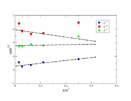
Figure 1: Masses of the lowest-lying glueballs for $N=2,3,4,6,8$, with their extrapolation to large $N$ [23].

We start from the computationally easier case of the pure Yang-Mills theory. Observables of interest in this case include masses of gauge-invariant states (glueballs). These are obtained from the large time behaviour of correlation functions of the form

$$C(t)=\langle O^{{\dagger}}(0)O(t)\rangle\mathop{\propto}^{t\to\infty}e^{-mt}\ ,$$ (12)

where $O$ is a traced product of links along a closed path ${\cal C}$ that transforms in an irreducible representation of angular momentum $J$ of the rotational group. For the definition of $C(t)$, the zero-momentum component (i.e. the spatial average) is taken. If the path is constructed in such a way that it has a definite parity $P$ and a charge conjugation eigenstate is constructed by taking either the real ($C=1$) or imaginary ($C=-1$) part of the trace, then $m$ is the lowest state in the $J^{PC}$ channel. In practice, after lattice discretisation, the group of rotations is broken to the dihedral group of rotations of the cube. Classifying the lattice states according to the irreducible representations of this group proves to give a cleaner signal in numerical simulations. The full rotational quantum numbers can be reconstructed by looking at the decomposition of the lattice rotational symmetry group under irreducible representations of $SO(3)$. Likewise, the signal over noise ratio is significantly improved if in any channel one measures more than one operator and for each operator its cross-correlations with all others at various $t$. This defines the correlation matrix

$$C_{lm}(t)=\langle O^{{\dagger}}_{l}(0)O_{m}(t)\rangle\ ,$$ (13)

where $l$ and $m$ label operators associated to two different paths. The eigenvalues of $C^{-1}(0)C(t)$ decay exponentially, with a rate controlled by the masses in the given channel. Hence, ordering the eigenvalues, it is possible to extract the mass of the groundstate and the mass of the first few excitations, in what can be regarded as a variational calculation, in which the eigenstates are found by minimising the hamiltonian over the variational basis provided by the paths. The number of excitations that one can extract and the accuracy of the masses crucially depend on the size of the variational basis and the choice of the operators. The procedure is described in more detail in [24, 25].

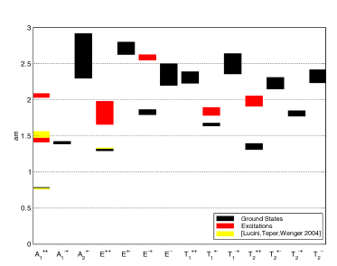
Figure 2: Large-$N$ extrapolation of the spectrum of glueballs at fixed lattice spacing corresponding to $aT_{c}=1/6$ (from [24]).

The continuum spectrum of the lowest-lying glueball was first extracted in [26]. In Fig. 1 we show the results of a more recent calculation [23]. The results for the $0^{++}$, its first excitation $0^{++*}$ and the $2^{++}$ glueballs can be summarised by the formulae

$$0^{++\phantom{*}}:\qquad\frac{m}{\sqrt{\sigma}} = 3.28(8)+\frac{2.1(1.1)}{N^{2}}\ ,$$

$$0^{++*}:\qquad\frac{m}{\sqrt{\sigma}} = 5.93(17)-\frac{2.7(2.0)}{N^{2}}\ ,$$ (14)

$$2^{++\phantom{*}}:\qquad\frac{m}{\sqrt{\sigma}} = 4.78(14)+\frac{0.3(1.7)}{N^{2}}\ .$$

Remarkably, only the leading correction in $1/N^{2}$ is needed to describe the data from $N=3$ to $N=8$, with a $\chi^{2}/\mathrm{dof}$ of order one, in a fit that gives coefficients of order one. This hints towards a well-behaved and convergent large-$N$ expansion. This result provides a quantification of the statement that $N=3$ is close to $N=\infty$: a correction $O(1/N^{2})$ accounts for the finite value of $N$ all the way down to $N=3$ with a level of precision of a few percents, which is the accuracy of our numerical data.

In order to gain more insight on the glueball spectrum, a more complete calculation exposing more excitations would be desirable. In order to eliminate possible sources of systematic effects, such a calculation should also be able to identify scattering states and contaminations from finite-size excitations related to loop wrapping around the periodic lattice (torelons). Although both effects disappear in the large-$N$ and large-volume limits, for a typical calculation their footprint can be non-negligible. A calculation of this type would require inserting in the variational basis operators corresponding to the unwanted states, which unavoidably increases the computational demands and the technical difficulties. A solution to the latter practical problems has been proposed in [24], where the construction of the basis operators has been fully automatised and hence it becomes easier to increase their number. The first results for the spectrum (this time at fixed lattice spacing) are reported in Fig. 2. An extrapolation to the continuum limit is currently being performed.

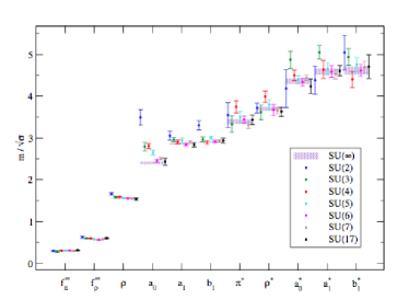
Figure 3: Mesonic observables at various values of $N$ and their large-$N$ extrapolation (from [27]).

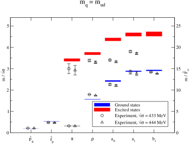
Figure 4: Comparison between lattice large-$N$ results and meson observables in QCD (from [30]).

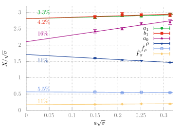
Figure 5: Estimate of lattice size corrections for various meson observables in SU(7) (from [30]).

For fermionic observables, all investigations performed so far are in the quenched approximation. Since this approximation is exact at $N=\infty$, it still allows us to obtain the correct values of observables in that limit. First results for the pseudoscalar and vector mesons at fixed lattice spacing were reported in [28, 29]. These studies were then extended to decay constants and other mesonic states in [27], with the continuum limit currently in progress (a status update is reported in [30]). A state of the art determination of the spectrum at various $N$ showing also the large-$N$ limit is given in Fig. 3.

In order to provide a qualitative picture of how close the large-$N$ limit is to real-world QCD, in Fig. 4 we show our numerical data together with experimental data at a quark mass set to its physical value by imposing that the ratio of the pion mass $m_{\pi}$ and of the pion decay constant $\hat{F}_{\pi}$ at $N=\infty$ is $m_{\pi}/\hat{F}_{\pi}=1.6$, i.e. compatible with the observed SU(3) value. In order to convert lattice units into MeV, a remaining ambiguity is the value of the string tension $\sqrt{\sigma}$ (for our calculation, $a\sqrt{\sigma}=0.095$). To give a handle on the connected systematics, two values of $\sqrt{\sigma}$ are reported in the figure. The lesson one learns is that the deviation of QCD from its large-$N$ limit is at most 5-7% for the lowest-lying meson spectrum and decay constants, while it can be larger (up to 20%) for excitations. However, concerning the latter remark, one has to consider that our lattice calculation has less control of systematic errors on excited states than it has on groundstates.

Another potential issue to consider are finite lattice spacing corrections. First results of a SU(7) study at various lattice spacings are shown in Fig. 5. For most of the states, corrections are of order 5% and below. However, it is interesting to note that the $\rho$ and the scalar meson $a_{0}$ have larger and opposite corrections that bring their masses close to each other. The degeneracy of the two states at large $N$ has been argued in [31]. This example shows that although in most of the cases we do not expect big surprises arising when taking the continuum limit, removing lattice spacing corrections in some few cases can prove to be crucial.

5 Conclusions and perspectives

The large-$N$ limit of SU($N$) gauge theories can help us to understand analytically non-perturbative results in QCD. In order to make progress with analytical calculations, lattice computations can be used as a reference. Two examples in different contexts on how lattice data can be used to inform analytical models are provided in [32, 6] (we refer to those works for further details). By now, there are various lattice calculations that provide increasingly solid results in the large-$N$ limit. In this short review, we have concentrated on the glueball and meson spectrum. For a wider overview of the field, we refer to [7, 8, 9].

References

- [1] G. ’t Hooft, A planar diagram theory for strong interactions, Nucl. Phys. B72 (1974) 461. doi:10.1016/0550-3213(74)90154-0.
- [2] J. M. Maldacena, The large N limit of superconformal field theories and supergravity, Adv. Theor. Math. Phys. 2 (1998) 231–252. arXiv:hep-th/9711200, doi:10.1023/A:1026654312961.
- [3] J. M. Maldacena, C. Núñez, Towards the large N limit of pure N=1 superYang-Mills, Phys.Rev.Lett. 86 (2001) 588–591. arXiv:hep-th/0008001, doi:10.1103/PhysRevLett.86.588.
- [4] I. R. Klebanov, M. J. Strassler, Supergravity and a confining gauge theory: Duality cascades and chi SB resolution of naked singularities, JHEP 0008 (2000) 052. arXiv:hep-th/0007191.
- [5] T. Sakai, S. Sugimoto, Low energy hadron physics in holographic QCD, Prog.Theor.Phys. 113 (2005) 843–882. arXiv:hep-th/0412141, doi:10.1143/PTP.113.843.
- [6] M. Bochicchio, Glueball and meson propagators of any spin in large-N QCD, Nucl.Phys. B875 (2013) 621–649. arXiv:1305.0273, doi:10.1016/j.nuclphysb.2013.07.023.
- [7] M. Panero, Recent results in large- lattice gauge theories, PoS Lattice 2012 (2012) 010. arXiv:1210.5510.
- [8] B. Lucini, M. Panero, SU(N) gauge theories at large N, Phys.Rept. 526 (2013) 93–163. arXiv:1210.4997, doi:10.1016/j.physrep.2013.01.001.
- [9] B. Lucini, M. Panero, Introductory lectures to large- QCD phenomenology and lattice results, Prog.Part.Nucl.Phys. 75 (2014) 1–40. arXiv:1309.3638, doi:10.1016/j.ppnp.2014.01.001.
- [10] S. R. Coleman, E. Witten, Chiral Symmetry Breakdown in Large N Chromodynamics, Phys.Rev.Lett. 45 (1980) 100. doi:10.1103/PhysRevLett.45.100.
- [11] A. V. Manohar, Large N QCD, (1998) 1091–1169arXiv:hep-ph/9802419.
- [12] R. F. Dashen, E. E. Jenkins, A. V. Manohar, The 1/N(c) expansion for baryons, Phys. Rev. D49 (1994) 4713. arXiv:hep-ph/9310379, doi:10.1103/PhysRevD.49.4713.
- [13] E. E. Jenkins, Baryon hyperfine mass splittings in large N QCD, Phys.Lett. B315 (1993) 441–446. arXiv:hep-ph/9307244, doi:10.1016/0370-2693(93)91638-4.
- [14] H. B. Nielsen, M. Ninomiya, Absence of Neutrinos on a Lattice. 1. Proof by Homotopy Theory, Nucl.Phys. B185 (1981) 20. doi:10.1016/0550-3213(81)90361-8.
- [15] G. ’t Hooft, Large N, arXiv:hep-th/0204069.
- [16] R. Narayanan, H. Neuberger, Chiral symmetry breaking at large N(c), Nucl.Phys. B696 (2004) 107–140. arXiv:hep-lat/0405025, doi:10.1016/j.nuclphysb.2004.07.002.
- [17] A. Hietanen, R. Narayanan, R. Patel, C. Prays, The vector meson mass in the large N limit of QCD, Phys. Lett. B674 (2009) 80–82. arXiv:0901.3752, doi:10.1016/j.physletb.2009.02.054.
- [18] A. González-Arroyo, M. Okawa, The string tension from smeared Wilson loops at large N, Phys.Lett. B718 (2012) 1524–1528. arXiv:1206.0049, doi:10.1016/j.physletb.2012.12.027.
- [19] T. Eguchi, H. Kawai, Reduction of Dynamical Degrees of Freedom in the Large N Gauge Theory, Phys.Rev.Lett. 48 (1982) 1063. doi:10.1103/PhysRevLett.48.1063.
- [20] G. Bhanot, U. M. Heller, H. Neuberger, The Quenched Eguchi-Kawai Model, Phys.Lett. B113 (1982) 47. doi:10.1016/0370-2693(82)90106-X.
- [21] A. González-Arroyo, M. Okawa, The Twisted Eguchi-Kawai Model: A Reduced Model for Large N Lattice Gauge Theory, Phys.Rev. D27 (1983) 2397. doi:10.1103/PhysRevD.27.2397.
- [22] R. Narayanan, H. Neuberger, Large N reduction in continuum, Phys.Rev.Lett. 91 (2003) 081601. arXiv:hep-lat/0303023, doi:10.1103/PhysRevLett.91.081601.
- [23] B. Lucini, M. Teper, U. Wenger, Glueballs and k-strings in SU(N) gauge theories: Calculations with improved operators, JHEP 0406 (2004) 012. arXiv:hep-lat/0404008, doi:10.1088/1126-6708/2004/06/012.
- [24] B. Lucini, A. Rago, E. Rinaldi, Glueball masses in the large N limit, JHEP 1008 (2010) 119. arXiv:1007.3879, doi:10.1007/JHEP08(2010)119.
- [25] B. Lucini, Glueballs from the Lattice, PoS QCD-TNT-III (2013) 023. arXiv:1401.1494.
- [26] B. Lucini, M. Teper, SU(N) gauge theories in four-dimensions: Exploring the approach to N = infinity, JHEP 0106 (2001) 050. arXiv:hep-lat/0103027.
- [27] G. S. Bali, F. Bursa, L. Castagnini, S. Collins, L. Del Debbio, et al., Mesons in large-N QCD, JHEP 1306 (2013) 071. arXiv:1304.4437, doi:10.1007/JHEP06(2013)071.
- [28] L. Del Debbio, B. Lucini, A. Patella, C. Pica, Quenched mesonic spectrum at large N, JHEP 0803 (2008) 062. arXiv:0712.3036, doi:10.1088/1126-6708/2008/03/062.
- [29] G. S. Bali, F. Bursa, Mesons at large N(c) from lattice QCD, JHEP 0809 (2008) 110. arXiv:0806.2278, doi:10.1088/1126-6708/2008/09/110.
- [30] G. S. Bali, L. Castagnini, B. Lucini, M. Panero, Large-N mesons, arXiv:1311.7559.
- [31] J. Nieves, E. Ruiz Arriola, Properties of the rho and sigma Mesons from Unitary Chiral Dynamics, Phys.Rev. D80 (2009) 045023. arXiv:0904.4344, doi:10.1103/PhysRevD.80.045023.
- [32] J. Erdmenger, N. Evans, I. Kirsch, E. Threlfall, Mesons in Gauge/Gravity Duals - A Review, Eur.Phys.J. A35 (2008) 81–133. arXiv:0711.4467, doi:10.1140/epja/i2007-10540-1.