Exploiting the Structure of Bipartite Graphs for Algebraic and Spectral Graph Theory Applications

Abstract

In this article, we extend several algebraic graph analysis methods to bipartite networks. In various areas of science, engineering and commerce, many types of information can be represented as networks, and thus the discipline of network analysis plays an important role in these domains. A powerful and widespread class of network analysis methods is based on algebraic graph theory, i.e., representing graphs as square adjacency matrices. However, many networks are of a very specific form that clashes with that representation: They are bipartite. That is, they consist of two node types, with each edge connecting a node of one type with a node of the other type. Examples of bipartite networks (also called two-mode networks) are persons and the social groups they belong to, musical artists and the musical genres they play, and text documents and the words they contain. In fact, any type of feature that can be represented by a categorical variable can be interpreted as a bipartite network. Although bipartite networks are widespread, most literature in the area of network analysis focuses on unipartite networks, i.e., those networks with only a single type of node. The purpose of this article is to extend a selection of important algebraic network analysis methods to bipartite networks, showing that many methods from algebraic graph theory can be applied to bipartite networks with only minor modifications. We show methods for clustering, visualization and link prediction. Additionally, we introduce new algebraic methods for measuring the bipartivity in near-bipartite graphs.

Introduction

The term network analysis refers to an area of research covering the social sciences, computer science, economy, and others. The analysis of networks is central to sociology, in which the relations between people are modeled as networks, as well as to recent studies of the World Wide Web, Web Science and others. The emerging field of Network Science is solely dedicated to the study of networks – owing its existence to the fact that a large number of diverse data can be modeled as networks: Not only ties between people, as in social networks, but also communication between people can be modeled as a network in which each act of communication is a link between two persons, transportation networks such as road, railroad and airport networks in which nodes are places and links represent transportation corridors, but also reference networks between publications or pages on the Web. Other examples are found in biology, where interactions between metabolites form a metabolic network, and in linguistics, where semantic relationships between words form a semantic network. Although they are taken from a highly diverse set of application areas, these examples all have in common the underlying model of a network: a set of nodes connected by links.

The advantages of network analysis become clear once we consider the breadth of mathematical tools available for analysing networks: From simple numerical characterizations of networks such as the clustering coefficient and the diameter to the analysis of distributions associated with a network such as the degree distribution, a single network analysis method can be applied to all types of networks, giving insight to any type of network, even those not envisioned by the developers of the original method. Another important class of network analysis methods is given by the specialized subfield of algebraic graph theory, in which graphs are analysed using algebraic methods. Its main tool consists in representing a graph by a matrix, and using matrix decompositions and other methods to derive properties of the network.

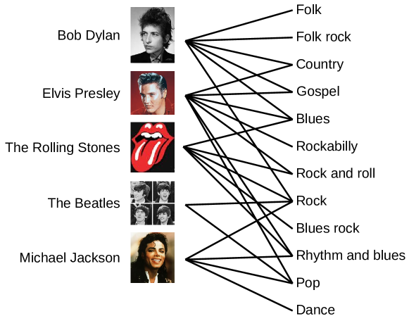
Although networks are ubiquitous in many areas, networks are not all similar: Many special types of networks exist, such as directed networks, signed networks, weighted networks, and so on. Although these networks have differing definitions, network analysis methods for simple networks can mostly be applied to them. For instance, instead of defining the adjacency matrix (which we will define in detail later) as a 0/1 matrix, it can be defined as an arbitrary matrix of reals, to which the same methods can be applied as in the simple case. One type of network however is more complex in its structure: bipartite networks. A bipartite network (also called two-mode network) is a network whose nodes can be partitioned into two sets, such that all links connect two nodes of different types. Ordinary networks such as social networks for instance are not bipartite, since they contain triangles. However, many other networks are bipartite. For instance, the well-know Southern Women dataset, consisting of information about women’s participation in social events in the Southern United States in the 1930s, is bipartite [14]. For another example, the set of connections between people and the things they like forms a bipartite network, consisting of person-nodes and thing-nodes, with each like connecting a person with a thing. Another example are the countries of origin of persons or things, the musical genres played by artists (as shown in Figure 1), the teams in which athletes have played, inclusion of people in social groups, tags assigned to documents (or any other kind of resource) and ratings given to movies (or other items). Other, less obvious examples are the words contained in text documents, in which the two node types are documents and words, and each link denotes the contains relationships. In fact, bipartite networks are a very important class of networks: Although the number cannot be taken as significant due to a clear sampling bias, the Koblenz Network Collection [33] contains, at the time of writing, 42% of bipartite networks (79 out of 189). A sample of bipartite network types is given in Table 1. A longer list is given in Table 5 in Appendix A.

The artist–genre network shown in Figure 1 is a subset of the actual Wikipedia genre information extracted by the DBpedia project [2], and will be used as a running example in the rest of this article. As a comparison, we will use a unipartite network containing tie of members of a karate club, taken from a well-known study by Wayne Zachary [55]. This small unipartite network contains 34 nodes and 78 edges.

A large part of the network analysis literature and methods only apply to unipartite networks, i.e., those networks having a single node type. Therefore, many studies project bipartite networks to unipartite networks, losing information in the process. To avoid this, unipartite algebraic graph analysis tools must be adapted, extended or completely redefined in the bipartite case. This has been done partially for some network analysis methods [8], although these methods do not exploit algebraic graph theory. This lack is the motivation of this article: to present a selection of the most important algebraic network analysis methods for bipartite networks.

Figure 1: An example of a bipartite graph: Musical artists and the genres they play. The network contains the two types of nodes artist and genre, and each edge connects a node of one type with a node of the other type.

Table 1: Examples of bipartite networks encountered in various areas.

Example	Node Types	References
Music genres	Artists + Genres	[2]
Starring	Actors + Movies	[22]
Sports	Players + Teams	[49]
Authorship	Authors + Works	[59]
Metabolism	Substances + Reactions	[28]
Ratings	Users + Items	[6, 10, 43]
Listening	Persons + Songs	[12]
Affiliation	Persons + Groups	[48]
Web analytics	Users + Web pages	[53]
Search engines	Queries + Clicked URLs	[47]
Economy	Producers + Consumers	[13]
Tag assignment	Items + Tags	[7]
Bag of words	Documents + Words	[30]
Taxonomy	Documents + Categories	[51]

The outline of the article is as follows:

• Section 1, Bipartite graphs: We give the definition of a bipartite network and review alternative representation of bipartite datasets other than through networks.

• Section 2, Algebraic graph theory: We review the usage of matrices to represent networks, requiring the replacement of the adjacency matrix with the biadjacency matrix. We show that paths between nodes in a bipartite network can be counted by computing alternating powers of the biadjacency matrix.

• Section 3, Measures of bipartivity: In the case where a network is not explicitly bipartite, it may be almost-bipartite. This section reviews algebraic measures of (non-)bipartivity, introducing several new ones.

• Section 4, Clustering analysis: This section describes spectral methods for detecting and measuring clustering in a network, i.e., the tendency of edges to form tight groups, as well as methods for finding such clusters.

• Section 5, Visualization: We describe methods for visualizing a bipartite network, showing that the bipartite structure is an additional type of information that can or cannot be visualized, reviewing advantages of both variants.

• Section 6, Link prediction: We treat the problem of link prediction, i.e., the prediction of links in evolving networks and show how common link prediction graph can be generalized to the bipartite case.

• Section 7, Other graph types: We review other graph types such as weighted and signed graphs, and their application to the bipartite case.

Throughout the paper, examples of bipartite networks will be taken from the Koblenz Network Collection [33], a collection of small and large networks of different types and from various application areas created by the authors. Section 6 (Link Prediction) is partly based on a previous paper of the author [35].

1 Bipartite Graphs

A network is an abstract structure consisting of nodes connected by links. Networks are modeled mathematically as graphs, which consist of a set of vertices (representing the nodes) connected by a set of edges (representing the links). A graph is usually denoted as

$$G=(V,E),$$

in which $G$ is the graph, $V$ is the set of vertices, and $E$ is the set of edges. An edge connecting the vertices $u,v\in V$ is denoted $\{u,v\}\in E$. The fact that two vertices $u$ and $v$ are connected will also be denoted $u\sim v$. The number of neighbors of a node $u$ is called the degree of $u$ and is denoted $d(u)=\{v\in V\mid u\sim v\}$.

Bipartite graphs are graphs in which the set of nodes can be partitioned into two disjoint sets such that each edge connects a vertex of one partition with a vertex of the other partition. A bipartite graph can be denoted as

$$G =(V_{1},V_{2},E),$$

in which $V_{1}$ and $V_{2}$ are the two disjoint vertex sets and $E$ is the set of vertices.

An equivalent characterization of bipartite graphs are the graphs that do not contain odd cycles, i.e., cycles consisting of an odd number of edges. In particular, it follows that a bipartite network does not contain triangles.

The term bipartite is sometimes employed in a slightly different way in mathematics and network science. Mathematically, any graph $G=(V,E)$ is by definition bipartite when a bipartition of $V$ exists, such that all edges in $E$ connect a vertex of one partition with a vertex of the other partition. In our notation however, a bipartition of the vertices will always be explicitly given by using the notation $G=(V_{1},V_{2},E)$. Thus, the term unipartite is not the exact opposite of bipartite: We call a network unipartite when it has a single node type, and links can connect any two nodes. This definition does not preclude a unipartite network from being bipartite in the mathematical sense. In the rest of the article, we will restrict usage of the term bipartite and unipartite to networks with two and one explicit node types. The two node sets $V_{1}$ and $V_{2}$ will be called the left and right edge sets.

Although bipartivity gives a special structure to a network, which can be exploited in various ways, we are not interested here in graphs that cannot be described as complex networks. For instance, a forest (i.e., a cycle-free graph) is bipartite in mathematical sense, but its structure is too trivial to be interesting in most cases.

1.1 Alternative Representations

An alternative representation of bipartite networks is as hypergraphs [58]. Let $G=(V_{1},V_{2},E)$ be a bipartite graph. Then we can construct its derived hypergraph $\mathrm{Hyp}(G)=(V_{1},F)$. As a reminder, the notion of hypergraph extends the notion of graph by allowing edges to connect any number of vertices, and are usually called hyperedges. By setting

$$F=(\{v\in V_{2}\mid\{u,v\}\in E\})_{u\in V_{1}},$$

we arrive at a hypergraph $H$ in which the left vertices of $G$ are the vertices, and the neighbors of each left node $u$ in $V_{1}$ make one hyperedge in $H$. In reverse, each hypergraph can be reduced to a bipartite graph in this way – another reason why bipartite graphs are important. As an example, a sets of groups formed by persons on a social networking site can be modeled as a hypergraph, in which the persons are the nodes, and each group gives one hyperedge making up all persons contained in that group. The equivalent bipartite graph has persons and groups as nodes, and an edge from a person to a group when the person is member of that group. Due to the symmetry between $V_{1}$ and $V_{2}$, we can build an analogous hypergraph representation $\mathrm{Hyp}(G)=(V_{2},F)$ in which $F$ contains one hyperedge for each node in $V_{1}$.

Another alternative way to model bipartite data is using the vector space model. This approach is very common in text mining, where documents containing words are modeled as word-vectors. Let $G=(V_{1},V_{2},E)$ be a bipartite document–word network, where $V_{1}$ are the documents and $V_{2}$ are the words. The vector space model then represents each document $u\in V_{1}$ as a vector $\mathbf{x}^{u}\in\mathbb{R}^{|V_{2}|}$ defined as

$$[\mathbf{x}^{u}]_{v} =\left\{\begin{array}[]{cc}1&\text{ when }\{u,v\}\in E\\ 0&\text{ when }\{u,v\}\notin E\end{array}\right.$$

In this representation, certain measures arise naturally, such as the cosine similarity. However, more complex methods are harder to recover. As an example, one may consider the cosine similarity, which measures the cosine of the angle between two vectors, or equivalently the dot product of two vectors, after a suitable normalization. By construction, the cosine similarity takes into account common words contained in two documents, but not more complex semantic relationships, such as synonyms. Instead, a graph-based similarity measure that considers paths in the bipartite document–word network will be able to find such relationships, as long as it is based on paths of length more than two between two documents.

Another common alternative representation of a bipartite network is by its projection to a unipartite network [50]. In the projection of a network onto the left nodes, only the left nodes are kept, and two nodes are connected when they have a common neighbor in the original bipartite graph. The projection onto the right nodes is defined analogously. Let $G=(V_{1},V_{2},E)$ be a bipartite graph. Then its projections to the left and right side can be defined as the graphs

$$G_{\mathrm{L}} =(V_{1},\{\{u,v\}\mid\exists w\in V_{2}:u\sim w,v\sim w\})$$

$$G_{\mathrm{R}} =(V_{1},\{\{u,v\}\mid\exists w\in V_{1}:u\sim w,v\sim w\})$$

The projections defined in this way are commonly used when unipartite network analysis methods are to be applied to bipartite networks. Among many examples, this is the case for edge types representing collaboration, whose name typically begin with co-, for instance, the co-authorship network of scientists or the co-starring network of actors. The projection networks however do not fully reflect the properties of the original bipartite networks. For instance, the left and right degree distributions in the original bipartite graph will by combined. However, the left and right degree distributions of bipartite networks are often very different, and this is lost in the projection.

1.2 Size, Volume and Fill

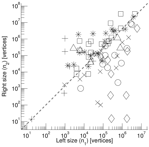
The size, volume and fill are three basic network characteristics that extend trivially to bipartite networks. The size denotes the number of nodes in a network. The size of a graph $G=(V,E)$ is $|V|$. For a bipartite graph $G=(V_{1},V_{2},E)$, the size is $|V_{1}|+|V_{2}|$, and we can distinguish between the left size $|V_{1}|$ and the right size $|V_{2}|$. The sizes of the left and right node sets can vary greatly. Figure 2 shows a scatter plot of the left and right node sets of all networks in the Koblenz Network Collection [33]. As an example for a very skewed bipartite network, the rating network of Netflix [6] contains 480,189 users but only 17,770 movies.

Figure 2: Comparison of the left and right network sizes (number of nodes) in bipartite networks of the Koblenz Network Collection [33]. Each letter code stands for one bipartite network.

The volume of a graph $G=(V,E)$ is its number of edges. For a bipartite graph $G=(V_{1},V_{2},E)$, no change in the definition is needed; the volume is simply $|E|$.

The fill of a network is the proportion of edges to the total amount of possible edges. In a unipartite graph $G=(V,E)$, the fill is given by $f=|E|/{|V|\choose 2}$. In a bipartite graph $G=(V_{1},V_{2},E)$, only edges between nodes in $V_{1}$ and nodes in $V_{2}$ are allowed, and thus the fill is given by $f=|E|/(|V_{1}||V_{2}|)$.

2 Algebraic Graph Theory

Algebraic graph theory is the branch of graph theory that represents graphs using algebraic structures in order to exploit the methods of algebra for graph theory. The main tool of algebraic graph theory is the representation of graphs as matrices, in particular the adjacency matrix and the Laplacian matrix. In the scope of this article, we will look at the adjacency matrix, since it has a special structure in the bipartite case, which can be exploited to give insights about path counts in the network. In the following, all matrices are real.

2.1 Adjacency Matrix

Given a unipartite graph $G=(V,E)$, its adjacency matrix $\mathbf{A}\in\mathbb{R}^{|V|\times|V|}$ is defined by

$$\mathbf{A}_{uv} =\left\{\begin{array}[]{lll}1&\text{when }\{u,v\}\in E\\ 0&\text{when }\{u,v\}\notin E\end{array}\right.$$

The adjacency matrix is square and symmetric, and has the useful property that it can be used to count paths in the network. It is easy to verify that the entry of the square of the adjacency matrix $[\mathbf{A}^{2}]_{uv}$ equals the number of common neighbors between the vertices $u$ and $v$, or equivalently the number of paths of length two between them. This result can be generalized to any power. For any $k\geq 0$, the number $[\mathbf{A}^{k}]_{uv}$ equals the number of paths of length $k$ between the nodes $u$ and $v$. Counting the number of paths between two nodes is a very useful tool in network analysis. For instance, it can be used to recommend new friends in a social network (the friend of a friend approach), or to compute the distances from one node to all other nodes.

Due to its structure, a bipartite graph $G=(V_{1},V_{2},E)$ has an adjacency matrix of the form

$$\mathbf{A} =\left[\begin{array}[]{cc}\mathbf{0}&\mathbf{B}\\ \mathbf{B}^{\mathrm{T}}&\mathbf{0}\end{array}\right],$$ (3)

in which $\mathbf{B}\in\mathbb{R}^{|V_{1}|\times|V_{2}|}$ is called the biadjacency matrix of $G$, and $\mathbf{0}$ are zero matrices of appropriate size. Because the biadjacency matrix is rectangular, we cannot simply take its powers to count paths in the network. However, we can derive a specific form of powers from its relation to the adjacency matrix, making a distinction between even and odd powers:

$$\mathbf{A}^{2k} =\left[\begin{array}[]{cc}(\mathbf{B}\mathbf{B}^{\mathrm{T}})^{k}&\mathbf{0}\\ \mathbf{0}&(\mathbf{B}^{\mathrm{T}}\mathbf{B})^{k}\end{array}\right],$$

$$\mathbf{A}^{2k+1} =\left[\begin{array}[]{cc}\mathbf{0}&(\mathbf{B}\mathbf{B}^{\mathrm{T}})^{k}\mathbf{B}\\ (\mathbf{B}^{\mathrm{T}}\mathbf{B})^{k}\mathbf{B}^{\mathrm{T}}&\mathbf{0}\end{array}\right].$$

From this we can derive expressions for path counts:

• The number of paths of length $2k$ between two nodes $u,v\in V_{1}$ equals $[(\mathbf{B}\mathbf{B}^{\mathrm{T}})^{k}]_{uv}$.

• The number of paths of length $2k$ between two nodes $u,v\in V_{2}$ equals $[(\mathbf{B}^{\mathrm{T}}\mathbf{B})^{k}]_{uv}$.

• The number of paths of length $2k+1$ between a node $u\in V_{1}$ and a node $v\in V_{2}$ is $[(\mathbf{B}\mathbf{B}^{\mathrm{T}})^{k}\mathbf{B}]_{uv}$.

All other path counts are zero due to the bipartite structure of the graph. Thus, all path counts in a bipartite graph can be computed using alternating powers of the biadjacency matrix, following the pattern $\mathbf{B}\mathbf{B}^{\mathrm{T}}\dotsm\mathbf{B}$.

2.2 Matrix Decompositions

A major advantage of representing networks as matrices is the possibility of exploiting matrix decompositions, which can be used to compute powers of matrices efficiently. In particular, two decompositions are used: the eigenvalue decomposition and the singular value decomposition.

Given a real symmetric matrix $\mathbf{X}\in\mathbb{R}^{n\times n}$, its eigenvalue decomposition is

$$\mathbf{X} =\mathbf{U}\mathbf{\Lambda}\mathbf{U}^{\mathrm{T}},$$

in which $\mathbf{U}$ is an orthogonal matrix of size $n\times n$ (meaning that $\mathbf{U}^{\mathrm{T}}\mathbf{U}=\mathbf{I}$) and $\mathbf{\Lambda}$ is a real diagonal matrix of size $n\times n$. The diagonal elements of $\mathbf{\Lambda}$ are called the eigenvalues of $\mathbf{X}$, and the columns of $\mathbf{U}$ are called its eigenvectors. The set of eigenvalues of a matrix are also called its spectrum. The multiplicity of an eigenvalue is defined as the number of times it occurs on the diagonal of $\mathbf{\Lambda}$.

Given any $m\times n$ real matrix $\mathbf{Y}$ (square or non-square, symmetric or asymmetric), its singular value decomposition is

$$\mathbf{Y} =\mathbf{U}\mathbf{\Sigma}\mathbf{V}^{\mathrm{T}},$$

in which $\mathbf{U}$ and $\mathbf{V}$ are orthogonal matrices of sizes $m\times m$ and $n\times n$, and $\mathbf{\Sigma}$ is a nonnegative diagonal $m\times n$ matrix. The diagonality of $\mathbf{\Sigma}$ is to be understood as all entries $\mathbf{\Sigma}_{ij}$ with $i\neq j$ are zero. The diagonal elements of $\mathbf{\Sigma}$ are called the singular values of $\mathbf{Y}$; the columns of $\mathbf{U}$ and $\mathbf{V}$ are called its left and right singular vectors.

The eigenvalue decomposition of a bipartite network’s adjacency matrix $\mathbf{A}$ is equivalent to the singular value decomposition of its biadjacency matrix $\mathbf{B}$. Given the singular value decomposition $\mathbf{B}=\mathbf{U}\mathbf{\Sigma}\mathbf{V}^{\mathrm{T}}$, the eigenvalue decomposition of $\mathbf{A}$ is given by

$$\mathbf{A} =\left[\begin{array}[]{cc}\mathbf{\bar{U}}&{\phantom{-}}\mathbf{\bar{U}}\\ \mathbf{\bar{V}}&-\mathbf{\bar{V}}\end{array}\right]\left[\begin{array}[]{cc}+\mathbf{\Sigma}&\\ &-\mathbf{\Sigma}\end{array}\right]\left[\begin{array}[]{cc}\mathbf{\bar{U}}&{\phantom{-}}\mathbf{\bar{U}}\\ \mathbf{\bar{V}}&-\mathbf{\bar{V}}\end{array}\right]^{\mathrm{T}},$$

with $\mathbf{\bar{U}}=\mathbf{U}/\sqrt{2}$ and $\mathbf{\bar{V}}=\mathbf{V}/\sqrt{2}$. In this decomposition, each singular value $\sigma$ corresponds to the eigenvalue pair $\{\pm\sigma\}$.

In order to compute powers of the adjacency matrix, a special property of the eigenvalue decomposition can be exploited. Using the eigenvalue decomposition $\mathbf{A}=\mathbf{U}\mathbf{\Lambda}\mathbf{U}^{\mathrm{T}}$, any power of the adjacency matrix can be computed as

$$\mathbf{A}^{k} =\mathbf{U}\mathbf{\Lambda}^{k}\mathbf{U}^{\mathrm{T}}.$$

This can be shown by using the fact the $\mathbf{U}$ is orthogonal, for instance, $\mathbf{A}^{2}=\mathbf{U}\mathbf{\Lambda}\mathbf{U}^{\mathrm{T}}\mathbf{U}\mathbf{\Lambda}\mathbf{U}^{\mathrm{T}}=\mathbf{U}\mathbf{\Lambda}\mathbf{\Lambda}\mathbf{U}^{\mathrm{T}}$. This form is convenient because powers of the diagonal matrix $\mathbf{\Lambda}$ can simply be computed by taking powers of its diagonal entries.

To compute alternating powers of the biadjacency matrix $\mathbf{B}$, its singular value decomposition can then be used in an analogous way. For instance,

$$\mathbf{B}\mathbf{B}^{\mathrm{T}}\mathbf{B} =\mathbf{U}\mathbf{\Sigma}\mathbf{V}^{\mathrm{T}}\mathbf{V}\mathbf{\Sigma}\mathbf{U}^{\mathrm{T}}\mathbf{U}\mathbf{\Sigma}\mathbf{V}^{\mathrm{T}}$$

$$=\mathbf{U}\mathbf{\Sigma}^{3}\mathbf{V}^{\mathrm{T}}.$$

This method can be used to compute any odd alternating power of $\mathbf{B}$.

2.3 Graph Laplacian

Beyond the adjacency matrix $\mathbf{A}$, another matrix is commonly used to analyse graphs algebraically: the Laplacian matrix $\mathbf{L}$. Let $G=(V,E)$ be a graph with adjacency matrix $\mathbf{A}$. Then, its degree matrix $\mathbf{D}$ is defined as the diagonal matrix containing the node degrees on the diagonal, i.e.

$$\mathbf{D}_{uu} =d(u).$$

The Laplacian matrix $\mathbf{L}$ is then the symmetric $|V|\times|V|$ matrix defined as $\mathbf{L}=\mathbf{D}-\mathbf{A}$. The Laplacian matrix has only nonnegative eigenvalues (it is positive-semidefinite), and its eigenvectors can be used for grouping the nodes of the graph into clusters, and also for graph drawing, as we will see in sections 4 and 5.

Unlike the adjacency matrix, the Laplacian matrix of a bipartite graph does not have a block structure akin to that given in Equation 3. Thus, we cannot define any corresponding rectangular bi-Laplacian matrix of which the singular value decomposition would give us information equivalent to the eigenvalue decomposition of the Laplacian $\mathbf{L}$ [23].

3 Measures of Bipartivity

Most bipartite networks are explicitly stored as such in information systems. For instance, any recommender system will have a clear distinction between users and items. In these cases, it is clear how to split the vertex set $V$ into $V_{1}$ and $V_{2}$. In other cases, the bipartition is not explicit, but implicit in the data. As an example, a dating website in which users can rate the profile of other users will have a majority of edges connecting men with women, and thus not be bipartite, but nearly so [37]. In this case, a bipartition would have to be inferred from the data. If the network is strictly bipartite, a bipartition can then be derived easily. If however, as is likely in the example of the dating website, the network is not quite bipartite, then that is not possible.

Almost-bipartite networks include networks of sexual contacts [42] and ratings on online dating sites [11, 37]. Other, more subtle cases, involve online social networks. For instance, the follower graph of the microblogging service Twitter is by construction unipartite, but has been observed to reflect, to a large extent, the usage of Twitter as a news service [40], as two types of users can be identified: those who primarily get followed (news sources) and those who primarily follow (readers). Thus, the Twitter follower graph is almost bipartite. Other social networks do not necessarily have a near-bipartite structure, but the question might be interesting to ask to what extent a network is bipartite. To answer this question, we need to define measures of bipartivity.

Instead of defining measures of bipartivity, we will instead consider measures of non-bipartivity, as these can be defined in a way that they equal zero when the graph is bipartite. Given an (a priori) unipartite graph $G=(V,E)$, a measure of non-bipartivity $b(G)$ characterizes the extent to which $G$ fails to be bipartite. In the following, we review four spectral measures of non-bipartivity, and compare them numerically on a large collection of example datasets. All four measures we present are nonnegative, and equal zero if and only if the graph is bipartite. The four measures are based on the three characteristic graph matrices $\mathbf{A}$, $\mathbf{N}$ and $\mathbf{K}$. Two of the measures are novel, and one is a novel algebraic relaxation of a known non-algebraic measure. All four measures are algebraic. Incidentally, we are not aware of a non-algebraic measure of (non-)bipartivity that is not covered by our four measures.

3.1 Frustration – Spectrum of $\mathbf{K}$

A first test of bipartivity consists in counting the minimum number of frustrated edges in a network [24, 56]. Given a bipartition $V=V_{1}\cup V_{2}$, a frustrated edge is an edge connecting two nodes in $V_{1}$, or two nodes in $V_{2}$. Let $f$ be the minimal number of frustrated edges in any bipartition of $V$. A measure of non-bipartivity is then given by the ratio of frustrated edges to total edges

$$b_{\mathrm{f}}(G) =\frac{f}{|E|}.$$

This measure is always in the range $[0,1/2]$. It attains the value zero if and only if $G$ is bipartite. The number of possible partitions $V=V_{1}\cup V_{2}$ in this minimization problem is exponential in the number of nodes, and thus the problem cannot be solved easily. Instead, it can be solved approximately using a Monte-Carlo algorithm. Alternatively, the minimal number of frustrated edges $f$ can be approximated by algebraic graph theory, in a way which we introduce below. First, we represent a bipartition $V=V_{1}\cup V_{2}$ by its characteristic node-vector $\mathbf{x}\in\mathbb{R}^{|V|}$ defined as

$$\mathbf{x}_{u} =\left\{\begin{array}[]{ll}+1/2&\text{when $u\in V_{1}$}\\ -1/2&\text{when $u\in V_{2}$}\end{array}\right.$$

Note that the frustration $f$, i.e., the number of edges within the sets $V_{1}$ and $V_{2}$ is then given by

$$f =\frac{1}{2}\sum_{(u,v)\in E}(\mathbf{x}_{u}+\mathbf{x}_{v})^{2}=\frac{1}{2}\mathbf{x}^{\mathrm{T}}\mathbf{K}\mathbf{x},$$

where $\mathbf{K}=\mathbf{D}+\mathbf{A}$ is the signless Laplacian matrix of the underlying unweighted graph. Thus, the minimal number of frustrated edges $f$ is given by

$$f =\min_{\mathbf{x}\in\{\pm 1/2\}^{|V|}}\frac{1}{2}\mathbf{x}^{\mathrm{T}}\mathbf{K}\mathbf{x}.$$

By relaxing the condition $\mathbf{x}\in\{\pm 1/2\}^{|V|}$, we can express $f$ in function of $\mathbf{K}$’s minimal eigenvalue, using the fact that the norm of all vectors $\mathbf{x}\in\{\pm 1/2\}^{|V|}$ equals $\sqrt{|V|/4}$, and the property that the minimal eigenvalue of a matrix equals its minimal Rayleigh quotient.

$$\frac{2f}{|V|/4} \approx\min_{\mathbf{x}\neq\mathbf{0}}\frac{\mathbf{x}^{\mathrm{T}}\mathbf{K}\mathbf{x}}{\left\|\mathbf{x}\right\|^{2}}=\lambda_{\min}[\mathbf{K}]$$

We can thus approximate the measure of non-bipartivity $b_{\mathrm{f}}$ by

$$b_{\mathrm{f}} \approx b_{\mathrm{K}}=\frac{|V|}{8|E|}\lambda_{\min}[\mathbf{K}]$$

Finally, we note that the eigenvalue $\lambda_{\min}[\mathbf{K}]$ can also be interpreted as the algebraic conflict in $G$ interpreted as a signed graph in which all edges have negative weight [34].

3.2 Spectrum of $\mathbf{A}$

The adjacency matrix $\mathbf{A}$ is symmetric and thus has real eigenvalues. In general, its eigenvalues are unbounded and can be positive and negative. When a network does not contain loops (edges from a node to itself), the trace of $\mathbf{A}$ and thus the sum of its eigenvalues is zero. However, the distribution of eigenvalues around zero is not symmetric in the general case. In fact, the eigenvalues are distributed in a symmetric way around zero if and only if the graph is bipartite. Thus, the eigenvalues of $\mathbf{A}$ can serve as a test of non-bipartivity in the following way: When a graph is bipartite, the smallest eigenvalue of the adjacency matrix equals the negative of the largest one, i.e., $\lambda_{\min}[\mathbf{A}]=-\lambda_{\max}[\mathbf{A}]$. If a graph is not bipartite, the smallest eigenvalue is nearer to zero, i.e., $\lambda_{\min}[\mathbf{A}]>-\lambda_{\max}[\mathbf{A}]$. Note that it is not possible that the smallest eigenvalue equals the largest in absolute value in a non-bipartite graph. Thus, the ratio of the smallest eigenvalue to its minimal value as a measure of non-bipartivity, which, when scaled accordingly, is zero if and only if the graph is bipartite.

$$b_{\mathrm{A}}(G) =1-\left|\frac{\lambda_{\min}[\mathbf{A}]}{\lambda_{\max}[\mathbf{A}]}\right|$$

This measure of non-bipartivity is always in the range $[0,1]$.

3.3 Spectrum of $\mathbf{N}$

Instead of measuring the non-bipartivity of a graph by the eigenvalues of its adjacency matrix $\mathbf{A}$, we can measure it by the eigenvalues of a normalized version of the adjacency matrix, the matrix $\mathbf{N}$. The normalized adjacency matrix $\mathbf{N}$ has the same structure as the adjacency matrix, but its entries are normalized by the node degrees. It is given by

$$\mathbf{N} =\mathbf{D}^{-1/2}\mathbf{A}\mathbf{D}^{-1/2}$$

or equivalently by

$$\mathbf{N}_{uv} =\left\{\begin{array}[]{ll}1/\sqrt{d(u)d(v)}&\text{ when $u$ and $v$ are connected}\\ 0&\text{ when $u$ and $v$ are not connected}\end{array}\right.$$

The normalized adjacency matrix $\mathbf{N}$ can replace the adjacency matrix $\mathbf{A}$ when a normalization of edge weights by degree is appropriate.

Due to the normalization, the eigenvalues of $\mathbf{N}$ have special properties. All eigenvalues of $\mathbf{N}$ are contained in the interval $[-1,+1]$, the maximum eigenvalue $\lambda_{\max}[\mathbf{N}]$ is always one, and the minimal eigenvalue $\lambda_{\min}[\mathbf{N}]$ equals negative one if and only if the network is bipartite. Thus, we propose as a measure of non-bipartivity

$$b_{\mathrm{N}}(G) =\lambda_{\min}[\mathbf{N}]+1.$$

This measure is always in the range $[0,1]$.

3.4 Odd Cycles

Another test for bipartivity consists in counting the cycles in the network. If a network is almost bipartite, there are much more cycles of even length than cycles of odd length. Thus, the proportion of odd cycles to the total number of cycles, appropriately weighted to avoid infinite cycle counts, can be used as a measure of non-bipartivity [18].

In this derivation, we consider cycles that may contain repeated nodes. A cycle of length $k$ is a sequence of $k$ nodes $(u_{1},u_{2},\ldots,u_{k})$ such that $u_{i}\sim u_{i+1}$ for $1\leq i<k$ and $u_{1}\sim u_{k}$. We thus consider cycles to have a distinct starting node and a direction. Given a graph $G$, let $P(k)$ be the number of cycles of length $k$ in $G$. Using the adjacency matrix $\mathbf{A}$ of $G$, we can express this as

$$P(k) =\mathrm{Tr}(\mathbf{A}^{k})$$

Then, a measure of non-bipartivity is given by the ratio of odd cycles to all cycles

$$b_{\mathrm{c}}(G) =\frac{\sum_{k=0}^{\infty}w(1+2k)P(1+2k)}{\sum_{k=0}^{\infty}w(k)P(k)}$$

$$=\frac{\sum_{k=0}^{\infty}w(1+2k)\mathrm{Tr}(\mathbf{A}^{1+2k})}{\sum_{k=0}^{\infty}w(k)\mathrm{Tr}(\mathbf{A}^{k})}$$

$$=\frac{\mathrm{Tr}(\sum_{k=0}^{\infty}w(1+2k)\mathbf{A}^{1+2k})}{\mathrm{Tr}(\sum_{k=0}^{\infty}w(k)\mathbf{A}^{k})}$$

This measure is dependent on a length-dependent cycle weight $w(k)$, without which both sums would diverge. Several choices for $w(k)$ are possible. We will consider here the weights $w(k)=1/k!$, resulting in the matrix exponential and hyperbolic sine:

$$b_{\mathrm{c}}(G) =\frac{\mathrm{Tr}(\sinh(\mathbf{A}))}{\mathrm{Tr}(\exp(\mathbf{A}))}$$

This can be expressed as a function of $\mathbf{A}$’s eigenvalues $\{\lambda_{k}\}$ as

$$b_{\mathrm{c}}(G) =\left(\sum_{k}\sinh(\lambda_{k})\right)/\left(\sum_{k}e^{\lambda_{k}}\right),$$

This measure is always in the range $[0,1/2]$, and attains the value of zero if and only if $G$ is bipartite.

3.5 Comparison

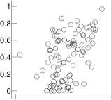
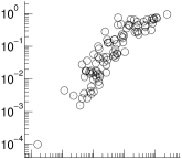
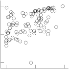
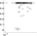
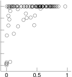
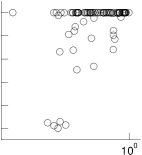
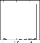
A comparison of the three measures of non-bipartivity is given in Table 2, and a numerical comparison of them is shown in Figure 3. A detailed comparison plot of the two measures $b_{\mathrm{A}}$ and $b_{\mathrm{N}}$ is shown in Figure 4. The numerical comparison shows that the values of $b_{\mathrm{c}}$ (the ratio of odd cycles) are in fact very near to $0.5$ for almost all networks, making the measure useless for characterizing large networks.

Figure 4 shows that bipartivity does not correlate with the type of network. While the most bipartite networks according to both measures are reference networks (the Notre Dame web (ND) and Baidu related pages (BAr)), other reference networks have very different non-bipartivity values. The same is also true for other network categories.

The runtimes needed to compute each of the four measures of non-bipartivity can be derived as follows. The fastest one to compute is the one based on the spectrum of the adjacency matrix $b_{\mathrm{A}}$, since we need only compute the maximum and minimum eigenvalues of $\mathbf{A}$, which can be done efficiently even for very large graphs. For $b_{\mathrm{N}}$, we must compute the minimum eigenvalue of the normalized adjacency matrix $\mathbf{N}$. Since $\mathbf{N}$’s eigenvalues are much less separated than $\mathbf{A}$’s, a power iteration on $\mathbf{N}$ takes longer than on $\mathbf{A}$. Computing the minimum eigenvalue of $\mathbf{K}$ is even slower, and needs more memory, as a sparse LU decomposition of $\mathbf{K}$ must be computed. Computing the measure $b_{\mathrm{c}}$ is high too, as it needs all eigenvalues of $\mathbf{A}$.

From the histograms shown in Figure 3, we can conclude that only $b_{\mathrm{A}}$ has an almost-uniform distribution, and thus we suppose it to be more informative. Since it also is the fastest of the measures to compute, we recommend to compute $b_{\mathrm{A}}$, i.e., $1-|\lambda_{\min}[\mathbf{A}]/\lambda_{\max}[\mathbf{A}]|$ as a measure of bipartivity for one-mode networks.

Table 2: Qualitative comparison of the four measures of non-bipartivity.

Measure	Measured feature	Range	Runtime
Frustration ($b_{\mathrm{K}}$)	Relaxed proportion of edges that must be removed to make the graph bipartite	$[0,1/2]$	Very high
Spectrum of $\mathbf{A}$ ($b_{\mathrm{A}}$)	Distance of smallest eigenvalue of the adjacency matrix to the opposite of the largest eigenvalue	$[0,1]$	Low
Spectrum of $\mathbf{N}$ ($b_{\mathrm{N}}$)	Distance of smallest eigenvalue of the normalized adjacency matrix to the opposite of the largest eigenvalue	$[0,1]$	Middle
Odd cycles ($b_{\mathrm{c}}$)	Proportion of odd cycles to total cycles, weighted by inverse factorial of cycle length	$[0,1/2]$	High

$b_{\mathrm{K}}$		$\rho=0.06$	$\rho=0.52^{***}$	$\rho=-0.08$
$b_{\mathrm{A}}$			$\rho=0.14$	$\rho=0.32^{**}$
$b_{\mathrm{N}}$				$\rho=0.11$
$b_{\mathrm{c}}$
	$b_{\mathrm{K}}$	$b_{\mathrm{A}}$	$b_{\mathrm{N}}$	$b_{\mathrm{c}}$

Figure 3: Quantitative comparison of the three measures of non-bipartivity. The diagonal subplots show histograms for each measure. The plots under the diagonal show scatter plots for each pair of measures. Over the diagonal, the Pearson correlation coefficients $\rho$ are shown, with $p$-values lower than 0.1, 0.01 and 0.001 shows as one, two and three stars.

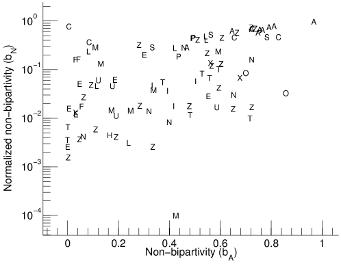
A Animal network C Human contact network E Metabolic network F Software network H Hyperlink network I Citation network L Lexical network M Communication network N Infrastructure network O Coauthorship network P Trophic network S Social network T Online contact network U Computer network X Miscellaneous network Z Online social network

Figure 4: All analysed networks plotted by the non-bipartivity measures $b_{\mathrm{A}}$ and $b_{\mathrm{N}}$. Each letter code stands for a single one-mode network. The individual letters correspond to the type of network.

4 Clustering Analysis

The term clustering refers to the observation that real-world networks, for instance social networks, tend to contain clusters, i.e., groups of nodes with a large number of edges among them, and few nodes connected to the outside of the group. A major problem class in machine learning, and indeed in unsupervised learning is the task of clustering. Given a set of data points and their attributes, the clustering problem asks to find subsets of these data points that are similar, in a way depending on the attributes. Examples of applications that can be reduced to clustering include community detection in social networks and the unsupervised determination of topics in a scientific collaboration graph.

The most general formulation of the clustering problem uses pairwise distances between the points. As an example, the $k$-means algorithm finds a partition of a set of points such that each point is nearest to the centroid of its assigned cluster.

If the points to be clustered are vertices in a graph, and the edges connecting the vertices are the only information available, then one speaks of graph clustering [44]. Of the many graph clustering methods in existence, we will review a spectral one that is both very general and which performs reasonably well in practice: ratio-cut spectral clustering. We will also restrict our treatment to the case of 2-clustering, i.e., finding a partition of the vertex set of a graph into two parts, such that each part contains as many edges as possible, and only few edges connect the two parts.

Let $G=(V,E)$ be a connected unipartite graph. Given any partition $V=X\cup Y$, the cut of the pair $(X,Y)$ is defined as the number of edges connecting $X$ and $Y$:

$$\mathrm{cut}(X,Y) =|\left\{u,v\in V\mid u\in X,v\in Y\right\}|$$

A good 2-clustering will thus give a low value of $\mathrm{cut}(X,Y)$. Using the cut as a minimization objective does not work however, since the result would be very skewed to partitions with one very small and one very large cluster. Thus, an suitable objective function for minimization is given by the ratio cut [44]

$$\mathrm{rcut}(X,Y) =\left(\frac{1}{|X|}+\frac{1}{|Y|}\right)\mathrm{cut}(X,Y).$$

The ratio cut can be minimized by expressing is in terms of the vector $\mathbf{x}\in\mathbb{R}^{|V|}$ defined by

$$\mathbf{x}_{u} =+\sqrt{|Y|/|X|}\text{ when }u\in X$$ (4)

$$\mathbf{x}_{u} =-\sqrt{|X|/|Y|}\text{ when }u\in Y.$$

Using the Laplacian matrix $\mathbf{L}\in\mathbb{R}^{|V|\times|V|}$ defined by $\mathbf{L}_{uu}=d(u)$, $\mathbf{L}_{uv}=-1$ when $u$ and $v$ are connected and $\mathbf{L}_{uv}=0$ otherwise, we can check that

$$\mathbf{x}\mathbf{L}\mathbf{x}^{\mathrm{T}} =2|V|\mathrm{rcut}(X,Y)$$

and that $\sum_{u}\mathbf{x}_{u}=0$, i.e., $\mathbf{x}$ is orthogonal to the constant vector. Denoting by $\mathcal{C}$ the vectors of the form given in Equation (4), the clustering problem becomes

$$\min_{\mathbf{x}\in\mathbb{R}^{|V|}} \quad\mathbf{x}\mathbf{L}\mathbf{x}^{\mathrm{T}}$$

$$\mathrm{s.t.} \quad\mathbf{x}\perp\mathbf{1},\mathbf{x}\in\mathcal{C}$$

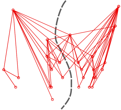
This can be relaxed by removing the constraint $\mathbf{x}\in\mathcal{C}$, giving as a solution the eigenvector of $\mathbf{L}$ having the smallest nonzero eigenvalue. The optimal $\mathbf{x}$ can then be used for 2-clustering, by defining the two clusters to comprise the nodes with positive and negative values in $\mathbf{x}$, respectively. Equivalently, the optimal $\mathbf{x}$ can be found by computing $\mathbf{x}=\mathbf{D}^{-1/2}\mathbf{y}$, where $\mathbf{D}$ is the diagonal degree matrix defined by $\mathbf{D}_{uu}=d(u)$, and $\mathbf{y}$ is the eigenvector corresponding to the second largest absolute eigenvalue of the matrix $\mathbf{D}_{1}^{-1/2}\mathbf{A}\mathbf{D}_{2}^{-1/2}$. Note that the largest eigenvalue of that matrix is one, and the corresponding eigenvector has entries inversely proportional to the vertex degrees. Here, $\mathbf{D}_{1}$ and $\mathbf{D}_{2}$ refer to the diagonal degree matrices computed from $\mathbf{D}$ by keeping all the left and right vertices, respectively. As an example, the resulting 2-clustering of Zachary’s unipartite karate club network is shown in Figure 5.

Figure 5: The optimal 2-clustering of Zachary’s unipartite karate club network, using the ratio cut criterion.

In the case of a bipartite graph $G(V_{1},V_{2},E)$, the problem of clustering is usually called biclustering or co-clustering [15]. These names refer to the fact that a good clustering of a bipartite graph must cluster both vertex sets in a way that is compatible with each other. In other words, the graph biclustering problem consists in finding the partitions

$$V_{1} =X_{1}\cup Y_{1},$$

$$V_{2} =X_{2}\cup Y_{2}.$$

In the case of the ratio cut, the objective is thus to minimize $\mathrm{rcut}(X_{1}\cup X_{2},Y_{1}\cup Y_{2})$. This can be realized by writing the network’s normalized adjacency matrix as

$$\mathbf{D}^{-1/2}\mathbf{A}\mathbf{D}^{-1/2} =\left[\begin{array}[]{cc}\mathbf{0}&\mathbf{D}_{1}^{-1/2}\mathbf{B}\mathbf{D}_{2}^{-1/2}\\ \mathbf{D}_{2}^{-1/2}\mathbf{B}^{\mathrm{T}}\mathbf{D}_{1}^{-1/2}&\mathbf{0}\\ \end{array}\right],$$

in which $\mathbf{B}$ is the biadjacency matrix of the network. It follows that a 2-clustering of a bipartite graph based on ratio cuts can be computed by finding the left and right singular vectors of the matrix $\mathbf{D}_{1}^{-1/2}\mathbf{B}\mathbf{D}_{2}^{-1/2}$ corresponding to the second-largest eigenvalue. As an example, the resulting 2-clustering of the bipartite artist–genre network is shown in Figure 6.

Figure 6: The optimal 2-clustering of the bipartite artist–genre network, using the ratio cut criterion.

4.1 Other Approaches

Another way to generalize the problem of graph clustering is by considering the concept of a clique. A clique in a graph is a set of nodes all of which are connected to each other. In other words, a clique is a complete graph $K_{n}$ that appears as a subgraph of another graph. In the bipartite case, the equivalent of a clique is a complete bipartite graph (or biclique) $K_{m,n}$ that appears as a subgraph. Now, a problem related to graph clustering is the problem of finding large cliques in a unipartite graph. Generalizing this to bipartite graphs results in the problem of finding large bicliques [32].

5 Visualization

Visualization is an important part of many exploratory sciences. Since so many different types of data can be modeled as networks, it is not surprising that network visualization constitutes a large topic. In fact, there are many different graph drawing algorithms, designed for many different types of networks, many of which can also be applied to bipartite networks. In this section, we describe one specific graph drawing algorithm that ties directly to our previous exposition about algebraic graph theory: spectral graph drawing, which consists in using the eigenvectors of characteristic graph matrices to draw a network. We note that other graph drawing algorithms exists, and also other settings in which they can be applied. However, we will restrict ourselves to the case of two-dimensional graph drawing, i.e., the embedding of the nodes of graph into a two-dimensional surface.

Let us begin by formalizing the graph drawing problem. Let $G=(V,E)$ be a graph. In order to draw $G$, we need to determine the coordinates of each node $u\in V$ in the drawing. The edges can then be drawn as lines from one node to another. For simplicity, we will restrict ourselves to graph drawing methods in which edges are drawn as straight lines. A graph drawing is by nature two-dimensional, and thus we must find a mapping of the nodes into the plane $\mathbb{R}^{2}$. We will represent this mapping by a matrix $\mathbf{X}\in\mathbb{R}^{|V|\times 2}$, in which each row $\mathbf{X}_{u:}$ represents the coordinates of node $u$.

A chosen graph drawing can be required to fulfill many aesthetic requirements, for instance that lines representing edges are not overlapping, that the drawing has constant density of nodes over the whole drawing, that cliques are apparent in the drawing, that nodes are not drawn too near to each other, etc. There are many such requirements, partially in conflict with each other. Any choice of such requirements (or rather, weighting of their importances), leads to a different graph drawing algorithm. The requirement chosen as an example in this section will be that of proximity: Nodes should be drawn near to their neighbors. We chose this requirement because it reflects the importance of the network structure over other aesthetic criteria, and because it leads to a closed-form solution with can be exploited in practice, in particular for very large networks.

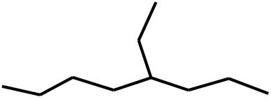
A second requirement which we will consider dictates that if a network has special structure, that structure should be reflected in the graph drawing. In the case of bipartite networks, this can for instance be achieved by placing all nodes on two parallel lines in the drawing, reflecting the two disjoint sets of nodes [20]. An illustration of such a drawing is shown in Figure 7, along with the example of a tree (a connected cycle-free graph) which is bipartite, but cannot be drawn in a nonintersecting manner when all nodes are placed on two lines. This example shows that aesthetic requirements can be in conflict with each other.

(a) Crossing-free drawing

(b) Highlighting the bipartite structure

Figure 7: An example of graph drawing that shows the conflict of aesthetic requirements: Drawing a tree (a connected cycle-free graph) can be done 7(a) without crossing edges but not showing the bipartite structure, or 7(b) showing the bipartite structure but including crossing edges. Note that it is impossible to fulfill both requirements at the same time for this graph, and therefore any bipartite graph drawing algorithm must choose which of these requirements will not be fulfilled in all cases.

In the rest of section, we first define the Laplacian-based graph drawing algorithm for unipartite graphs, and then show how it can be extended to the case of bipartite graphs, with and without the requirement to place the nodes on two parallel lines.

5.1 Spectral Drawing of Unipartite Graphs

We now describe the general method for generating an embedding of the nodes of a graph into the plane using the Laplacian matrix. Given a connected graph $G=(V,E)$, its adjacency matrix $(\mathbf{A}_{uv})$ gives the positive edge weights when the vertices $u$ and $v$ are connected, and is zero otherwise. We now want to find a two-dimensional drawing of the graph in which each vertex is drawn near to its neighbors. This requirement gives rise to the following vertex equation, which states that every vertex is placed at the mean of its neighbors’ coordinates, weighted by the weight of the connecting edges. For each node $u$, let $\mathbf{X}_{u:}\in\mathbb{R}^{2}$ be its coordinates in the drawing, then

$$\mathbf{X}_{u:} =\left(\sum_{v\sim u}\mathbf{A}_{uv}\right)^{-1}\sum_{v\sim u}\mathbf{A}_{uv}\mathbf{X}_{v:}.$$

Rearranging and aggregating the equation for all $u$ we arrive at

$$\mathbf{D}\mathbf{X} =\mathbf{A}\mathbf{X}$$

$$\mathbf{L}\mathbf{X} =\mathbf{0}$$

In other words, the columns of $\mathbf{X}$ should belong to the null space of the Laplacian matrix $\mathbf{L}$, which leads to the degenerate solution of $\mathbf{X}$ containing constant vectors, as the constant vector is an eigenvector of $\mathbf{L}$ with eigenvalue $0$. To exclude that solution, we require additionally that the column vectors of $\mathbf{X}$ are orthogonal to the constant vector and to each other, leading to the columns of $\mathbf{X}$ being the eigenvectors associated with the two smallest eigenvalues of $\mathbf{L}$ different from zero. This solution results in a well-known satisfactory embedding of positively weighted graphs:

$$\mathbf{X}_{:1} =\mathbf{x}_{2}[\mathbf{L}]$$

$$\mathbf{X}_{:2} =\mathbf{x}_{3}[\mathbf{L}]$$

where $\mathbf{x}_{k}[\mathbf{L}]$ denotes the eigenvector corresponding to the $k$’s smallest eigenvalue of $\mathbf{L}$. Such an embedding is related to the resistance distance (or commute time distance) between nodes of the graph [5].

As an example of this method, we show the spectral drawing of Zachary’s unipartite karate club network and of the United States power grid network [54] in Figure 8, showing that the method can be applied to both small and large networks.

(a) Zachary’s karate club

(b) U.S. power grid

Figure 8: Spectral graph drawings of two unipartite networks. 8(a) Zachary’s karate club, 8(b) the United States power grid (drawn without the edges for clarity). Both networks are drawn using the two eigenvectors of smallest nonzero eigenvalue of the Laplacian matrix $\mathbf{L}$.

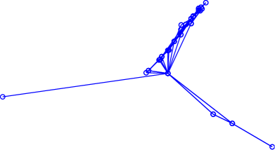
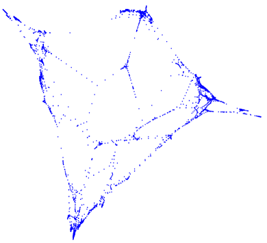
5.2 Spectral Drawing of Bipartite Graphs

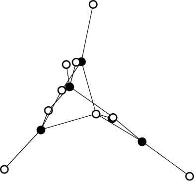
The spectral graph drawing method introduced previously can be applied to bipartite graphs, giving drawings where the nodes of the two types are mixed in the plane. An example for our small bipartite example subset of the artist–genre network, as well as for the full artist–genre network are shown in Figure 9.

(a) Subset of artist–genre network

(b) Full artist–genre network

Figure 9: Spectral graph drawings of the bipartite artist–genre network. 9(a) small example subset, 9(b) full network (drawn without the edges for clarity). Both networks are drawn using the two eigenvectors of smallest nonzero eigenvalue of the Laplacian matrix $\mathbf{L}$.

Alternatively, we may want to emphasize the bipartite structure in the network. Therefore, instead of using two eigenvectors of the Laplacian matrix $\mathbf{L}$, we only use one. The coordinates for the other dimension are then given by the bipartition:

$$\mathbf{X}_{:1} =\mathbf{x}_{2}[\mathbf{L}]$$

$$\mathbf{X}_{u2} =\left\{\begin{array}[]{ll}+1&\text{ when }u\in V_{1}\\ -1&\text{ when }u\in V_{2}\end{array}\right.$$

Note that this kind of bipartite graph drawing only makes sense when the edges are shown. If, as we did with the large artist–genre and power grid networks, edges are not shown, the drawing becomes uninformative since it only consist of two lines of points. The drawing is shown for the small bipartite artist–genre subset in Figure 10. As expected, the bipartivity of the network becomes apparent from the graph drawing, and the placement of the nodes on the two lines is such that clusters are apparent, for instance the seven nodes at the right of the drawing.

Figure 10: Drawing of the small bipartite artist–genre network that makes apparent the bipartite structure. Artists are shown as empty circles and genres as full circles.

In order to make apparent the bipartite structure of a network, other methods exist beyond the two-line model, for instance drawing vertices in two regions [57] or using a radial layout [17].

6 Link Prediction

The problem of link prediction covers a set of related problems that arise in various areas, which can all be formulated as the task of predicting links in a network. For instance, a social recommender system such as the You may know these persons feature on Facebook can be implemented by predicting new friendship ties in the Facebook social graph. Another application consists in finding researchers similar to a given one based on their collaboration graph. Yet another application consists in predict the sign of edges in a signed social network, i.e., a social network such as Slashdot [39] in which both friend and foe ties are allowed. All these applications are of the same form, in which a graph as well as two nodes are given, and a score must be computed for them.

The link prediction problem can be applied to bipartite networks, too. For instance, recommending items on Facebook based on the user–item like graph amounts to predicting links in that graph. A related task is collaborative filtering, i.e., the prediction of ratings in the bipartite user–item rating graph. This task differs from the pure link prediction task, because edges are weighted by ratings, and the goal is not to find edges, but to predict their weight. Nonetheless, the task can be implemented by the same methods used for link prediction.

The link prediction problem as defined here is very general, and plays a central role in the areas of information retrieval (mainly through word–document links), recommender systems (mainly through user–item links) and other domains. Thus, the number of previously described approaches is very large, and we only cover here a small representative subset of them which have algebraic formulations: preferential attachment, the common neighbors count, and various graph kernels.

A recommender can take several forms, not only by the type of network it operates on, but also with regard to whether it finds nodes, edges or computes probabilities. In our experiments, we will use the most general approach: returning a score when given a node pair. Thus, all link prediction algorithms for a graph $G=(V,E)$ will be formulated in terms of a score function $f:|V|^{2}\rightarrow\mathbb{R}$ that takes two vertices as input, and returns a real number. We do not pose any numerical constraint on the returned values; they could be probabilities, counts, or even negative values. The only rule is that a higher value denotes a higher probability of link formation.

6.1 Preferential Attachment

Preferential attachment refers to the idea that when a link is created in a network, it is more likely to attach to nodes that already have a high degree. More precisely, the probability that a new link attaches to a node $u$ can be modeled to be proportional to the degree $d(u)$. When taken as the only link formulation rule, this leads to the Barabási–Albert graph model. As a solution to the link prediction problem, preferential attachment can be used to derive the link prediction function [3]

$$f_{\mathrm{PA}}(u,v) =d(u)d(v).$$

This is arguably the simplest nontrivial link prediction function possible; it only takes vertex degrees into account, not the network structure. In fact, if we chose any vertex $u$, compute this function for the pairs $(u,v)$ for all $v\in|V|$, and then rank all vertices $v$ by score, the result will be independent of the initial vertex $u$. Thus, the preferential attachment link prediction function corresponds to the most popular recommender, i.e., a non-personalized recommender function. In the example of a friend recommender for a social network, the preferential attachment function always recommends the users with highest number of friends.

Even though it is rudimentary, the preferential attachment link prediction function can give reasonable results in many applications, and has the advantage to generalize trivially to bipartite networks: We can use its definition directly in a bipartite network without any modification. Other, more complex link prediction functions however are not that simple and will need adjustment for bipartite networks, since they are defined in terms of the underlying network structure.

6.2 Neighborhood-based Methods

Beyond preferential attachment, the simplest link prediction functions that are not independent on a source vertex are based on the principle of triangle closing [41]. For instance, the common neighbors count consists in counting the number of common neighbors between two given nodes, and is based on the observation that an edge joining two nodes with a high number of common neighbors will add many triangles to the graph. In the example of a friend recommender, this corresponds to the friend of a friend model, in which we recommend the users with which we have the highest number of common friends, but who are not our friends yet:

$$f_{\mathrm{CN}}(u,v) =|\{w\in V\mid u\sim w,v\sim w\}|$$

While this link prediction function takes into account the underlying network structure, it is useless for bipartite networks. In fact, new edges in a bipartite network always connect two vertices from different partitions, and cannot have common neighbors. In other words, triangle closing does not apply to bipartite networks, since bipartite networks do not contain triangles. However, since the common neighbor count is equal to the number of paths of length two between two nodes, we can switch to using the number of paths of length three as a bipartite link prediction function, which respects the bipartite network structure:

$$f_{\mathrm{P3}}(u,v) =|\{w,x\in V\mid u\sim w,w\sim x,x\sim v\}|$$

As shown in Section 2, this can be expressed using the biadjacency matrix as $f_{\mathrm{P3}}(u,v)=[\mathbf{B}\mathbf{B}^{\mathrm{T}}\mathbf{B}]_{uv}$.

A certain number of other link prediction functions are similar to the common neighbors count, but use normalization or multiplicative factors in various ways. These include the Jaccard index [41], the cosine similarity [45], and the measure of Adamic and Adar [1]. The extension of these measures to bipartite graphs can be done in various ways, depending on the generalization of the specific normalization method.

6.3 Graph Kernels

As an example of a class of more advanced link prediction functions, we review graph kernels. In a unipartite graph $G=(V,E)$, a graph kernel is a function of two vertices $k:|V|^{2}\rightarrow\mathbb{R}$ which is a kernel, i.e., the following properties hold:

• It is symmetric: $k(u,v)=k(v,u)$

• It is positive semidefinite: For any vector $\mathbf{x}\in\mathbb{R}^{|V|}$, $k$’s bilinear form is nonnegative, i.e., $\sum_{u,v\in V}\mathbf{x}_{u}k(u,v)\mathbf{x}_{v}\geq 0$.

A graph kernel thus has the same form as a link prediction function, but with the additional condition of being symmetric and positive-semidefinite. Graph kernels can be defined algebraically using the adjacency matrix and the Laplacian matrix, as in the examples given in Table 3.

Table 3: Examples of graph kernels that apply to unipartite networks.

Name	Expression
Neumann kernel [29]	$k_{\mathrm{NEU}}(u,v)=[(\mathbf{I}-\alpha\mathbf{A})^{-1}]_{uv}$
Exponential kernel [31]	$k_{\mathrm{EXP}}(u,v)=[e^{\alpha\mathbf{A}}]_{uv}$
Commute-time kernel [19]	$k_{\mathrm{COM}}(u,v)=[\mathbf{L}^{+}]_{uv}$
Heat diffusion kernel [27]	$k_{\mathrm{HEAT}}(u,v)=[e^{-\alpha\mathbf{L}}]_{uv}$

These graph kernels can be generalized to bipartite graphs. As an example, the exponential kernel can be generalized to the hyperbolic sine pseudokernel, and the special bipartite network structure can be exploited to compute it. The exponential kernel can be written as a power sum:

$$e^{\alpha\mathbf{A}} =\mathbf{I}+\alpha\mathbf{A}+\frac{\alpha^{2}}{2}\mathbf{A}^{2}+\frac{\alpha^{3}}{6}\mathbf{A}^{3}+\dotsb$$

In this form, it is clear that the exponential of the adjacency matrix equals a sum over all paths between two nodes, weighted by a decreasing function $\alpha^{k}/k!$ of the path length $k$. Thus, the exponential function enjoys two useful properties as a link prediction function:

• It is higher when there are more paths connecting two nodes.

• It is lower when the connecting paths are long.

These two properties are very useful for a unipartite link prediction function. For a bipartite link prediction function, the second property is counterproductive. Instead, only paths of odd length should be counted, and paths of even length have weighted zero. This is because a new edge in a bipartite network can only connect two nodes from different partitions in the network, and thus pre-existing paths connecting them must have odd length. Thus, the corresponding graph kernel for bipartite graphs is given by a reduction of the matrix exponential to only its odd terms; this is exactly the matrix hyperbolic sine [35]:

$$k_{\mathrm{SINH}} =\sinh(\alpha\mathbf{A})=\alpha\mathbf{A}+\frac{\alpha^{3}}{6}\mathbf{A}^{3}+\frac{\alpha^{5}}{120}\mathbf{A}^{5}+\dotsb$$

This function however is not a kernel, since it is not positive semidefinite – which is reflected by the fact the hyperbolic sine takes on negative values, unlike the exponential. Therefore, the resulting link prediction function is only a pseudokernel, i.e., a kernel without the positive-semidefinite property.

Both the exponential kernel and the hyperbolic sine pseudokernel can be computed efficiently using matrix decompositions. From its expression as a power sum, it can be seen that the matrix exponential can be written with help of the eigenvalue decomposition $\mathbf{A}=\mathbf{U}\mathbf{\Lambda}\mathbf{U}^{\mathrm{T}}$:

$$e^{\alpha\mathbf{A}} =\mathbf{U}e^{\alpha\mathbf{\Lambda}}\mathbf{U}^{\mathrm{T}}$$

Analogously, the hyperbolic sine can be written with help of the singular value decomposition of the biadjacency matrix $\mathbf{B}=\mathbf{U}\mathbf{\Sigma}\mathbf{V}^{\mathrm{T}}$:

$$\sinh(\alpha\mathbf{A}) =\left[\begin{array}[]{cc}\mathbf{0}&\mathbf{U}\sinh(\alpha\mathbf{\Sigma})\mathbf{V}^{\mathrm{T}}\\ \mathbf{V}\sinh(\alpha\mathbf{\Sigma})\mathbf{U}^{\mathrm{T}}&\mathbf{0}\end{array}\right]$$

Analogously, we can derive a bipartite version of the Neumann kernel. The Neumann kernel is defined as

$$(\mathbf{I}-\alpha\mathbf{A})^{-1} =\mathbf{I}+\alpha\mathbf{A}+\alpha^{2}\mathbf{A}^{2}+\dotsb$$

and, similarly to the exponential kernel, it assigns decreasing weights to increasing path lengths. By keeping only the odd terms we arrive at the odd Neumann kernel [29]:

$$k_{\mathrm{NEU}} =\alpha\mathbf{A}+\alpha^{3}\mathbf{A}^{3}+\alpha^{5}\mathbf{A}^{5}+\dotsb=\alpha\mathbf{A}(\mathbf{I}-\alpha^{2}\mathbf{A}^{2})^{-1}$$

The same strategy can be used for other graph kernels based on the adjacency matrix, for instance those learned from historical data [38]. These kernels can also be applied to the normalized adjacency matrix $\mathbf{N}$ and to the graph Laplacian $\mathbf{L}$ [4, 47, 52].

6.4 Evaluation

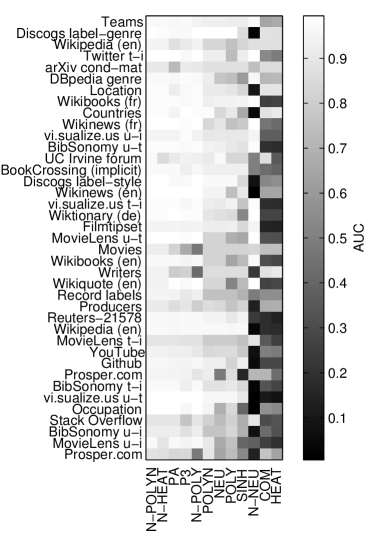
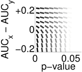
We perform an evaluation of the described link prediction algorithms on bipartite networks from the Koblenz Network Collection. The link prediction methods we used are summarized in Table 4, and the list of networks on which we make our experiments is given in Appendix A. We use the following methodology: For each network, we divide the set of edges into a training set (75% of edges) and a test set (25% of edges). Additionally, a zero test set of unconnected node pairs is created, having the same size as the test set. When edge arrival times are known for one network, the split is such that all training edges come before test edges. We then use the various methods shown in Table 4 to compute link prediction scores for all node pairs in the test set and zero test set. The scores are then used to compute the area under curve (AUC) as a measure of precision for each method [9]. AUC values range from zero to one, with higher values denoting better ranking. The results are shown in Figure 11.

Table 4: List of bipartite link prediction methods used in our experiments.

	Name	Expression
PA	Preferential attachment	$d(u)d(v)$
P3	Paths of length three	$|\{u\sim x\sim y\sim v\}|$
POLY	Odd polynomial of the adjacency matrix	$P_{\mathrm{o}}(\mathbf{A})$
POLYN	Odd nonnegative polynomial of the adjacency matrix	$P_{\mathrm{on}}(\mathbf{A})$
NEU	Odd Neumann kernel	$\alpha\mathbf{A}(\mathbf{I}-\alpha^{2}\mathbf{A}^{2})^{-1}$
SINH	Hyperbolic sine	$\sinh(\alpha\mathbf{A})$
N-POLY	Odd polynomial of the normalized adjacency matrix	$P_{\mathrm{o}}(\mathbf{N})$
N-POLYN	Odd nonnegative polynomial of the normalized adjacency matrix	$P_{\mathrm{on}}(\mathbf{N})$
N-NEU	Normalized odd Neumann kernel	$\alpha\mathbf{N}(\mathbf{I}-\alpha^{2}\mathbf{N}^{2})^{-1}$
N-HEAT	Normalized heat diffusion kernel	$\sinh(\alpha\mathbf{N})$
COM	Commute-time kernel	$\mathbf{L}^{+}$
HEAT	Heat diffusion kernel	$\exp(-\alpha\mathbf{L})$

Figure 11: Comparison of link prediction algorithms for bipartite networks. Left: the area under curve (AUC) for all methods and all networks. Right: pairwise comparison of performances, showing the p-value of the comparison as well as the average difference in AUC values.

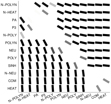Our experiments show that not all link prediction methods generalize well to bipartite networks. First, we see that the two methods based on the Laplacian matrix, the heat diffusion kernel and the commute-time kernel, perform very badly. The best results are in fact achieved by two functions of the normalized adjacency matrix: the polynomial and the normalized heat diffusion kernel. The normal Neumann kernel however does not perform well. In a similar vein to unipartite networks, we must conclude that there is no generally best method, and that the performance can vary from dataset to dataset as it does from method to method.

7 Other Graph Types

Graphs as defined in the previous sections of this article are generally called simple graphs, as they allow only single edges between two vertices. Their edges are undirected and unweighted. The archetypal example of a network modeled as a simple graph is a social network: persons connected by friendships. This definition can be extended to include multiple edges between a single vertex pair, weighted edges, signed edges, and directed edges. Of these extensions, all can be applied to bipartite graphs. In this section, we briefly review two of these extensions and their implications for algebraic graph theory: weighted graphs and directed graphs.

Edge Weights

A common feature of graphs are edge weights, which come in multiple forms. For one, edges can be directly weighted by a real number, such as in the trust network of the Advogato online community, in which three levels of trust exist, represented by the numbers 0.6, 0.8 and 1.0 [46]. Another type of weight is given by signed networks, in which positive and negative edges exist. An example is the Slashdot Zoo social network, in which people are related by friend and foe links [39]. Finally, networks may allow multiple parallel edges, in which case we may model the number of parallel edges as an integer weight. An example is an email network, with each edge representing an email between two persons. All these types of weightings can be applied to bipartite networks directly, giving a weighted biadjacency matrix $\mathbf{B}$. This matrix can then be used for any algebraic graph analysis method trivially.

Directed Graphs

In directed graphs, each edge has an orientation. Instead of being defined as the unordered set $\{u,v\}$, an edge in a directed network is defined as the ordered pair $(u,v)$. Edges in a directed graph are also called arcs. An example for a directed graph is the Twitter follower graph, consisting of Twitter users and their follow relationships [40]. The fact that user $u$ follows user $v$ can be represented by the directed edge $(u,v)\in E$. Arguably, more directed than undirected unipartite networks exist; in the Koblenz Network Collection for instance, 62% of all unipartite networks are directed [33]. On the other hand, directed bipartite graphs are very rare. They occur for instance in Petri nets, where the node types are places and transitions. Out of 189 networks in the Koblenz Network Collection as of 2014, not a single one is directed and bipartite.

Directed graphs can be transformed into bipartite graphs, using the bipartite double cover [16]. This gives a bipartite graph in which each edge corresponds to an original directed edge, and the set of vertices is doubled, as shown in Figure 12.

Figure 12: Illustration of the bipartite double cover, which generates an undirected bipartite graph from any directed unipartite graph.

Formally, the directed graph $G=(V,E)$ has the bipartite double cover

$$H =(V\times\{1,2\},\{\{(u,1),(v,2)\}\mid(u,v)\in E\}).$$

This mapping does not preserve the complete directed structure, because directed paths of the form $u\rightarrow v\rightarrow w$ are not reflected as paths in the bipartite double cover; only alternating paths are preserved, i.e., paths consisting of edges in alternating orientations relative to the path such as $u\rightarrow v\leftarrow w\rightarrow x$. If $\mathbf{B}$ is the adjacency matrix of a directed graph, then $\mathbf{B}$ is also the biadjacency matrix of its double cover, whose adjacency matrix is

$$\left[\begin{array}[]{cc}\mathbf{0}&\mathbf{B}\\ \mathbf{B}^{\mathrm{T}}&\mathbf{0}\end{array}\right].$$

An example in which these properties of the bipartite double cover are exploited are rating networks of online dating websites [37].

Conclusion

The topic of algebraic graph theory for bipartite networks is vast, and, as we have seen, specific analysis methods can be defined for many applications. In most cases, analysing a bipartite network does not just mean applying regular network analysis methods to a network that happens to the bipartite. Instead, specialized algebraic methods exist, that are both more efficient and better suited to the bipartite structure. A general pattern that we have exploited is the replacement of the square and symmetric adjacency matrix $\mathbf{A}$ with the rectangular biadjacency matrix $\mathbf{B}$. This construction leads to changes in its applications. For instance, the eigenvalue decomposition must be replaced by the singular value decomposition, which naturally maps to bipartite graphs, and the exponential kernel must be replaced by the hyperbolic sine pseudokernel. We also note that the existence of a match between the singular value decomposition and bipartite graphs is not trivial, in that there are examples of graphs with special structure that do not allow such a mapping: Directed networks for instance are represented naturally by asymmetric and square adjacency matrices, for which no extension of the eigenvalue decomposition is satisfactory, as shown in [36]: the asymmetric eigenvalue decomposition is not defined in the general case and discards information about when it is defined, the singular value decomposition of the asymmetric adjacency matrix implicitly applies to the bipartite double cover and thus loses information, and an alternative decomposition (DEDICOM) is computationally complex and non-unique.

The concept of bipartite networks itself can be generalized to $k$-partite networks. There are two different ways of achieving this: First, by letting each edge connect one vertex of every of the $k$ vertex sets, resulting in a $k$-regular hypergraph. This approach is taken for instance in the modeling of broad folksonomies, in which each tag assignment consists of a user–item–tag triple [26]. The second generalization of bipartite networks also allows any of $k$ different vertex types, and also $l$ different edge types, each edge type connecting two specific vertex types (which may be the same) [25]. This approach is taken in semantic networks, where each edge type then corresponds to one semantic predicate.

Appendix A Appendix: Networks

The list of networks used in the experiments in this paper is given in Table 5. All networks are available online with the Koblenz Network Collection [33].

Table 5: The bipartite networks used in this article.

Network $\boldsymbol{|V|}$ $\boldsymbol{|E|}$ Nodes Edges BibSonomy t-i $972{,}120$ $2{,}555{,}080$ Tag + Publication Assignment BibSonomy u-i $773{,}241$ $2{,}555{,}080$ User + Publication Tag assignment BibSonomy u-t $210{,}467$ $2{,}555{,}080$ User + Tag Assignment BookCrossing (implicit) $445{,}801$ $1{,}149{,}739$ User + Book Rating CiteULike u-t $175{,}992$ $2{,}411{,}819$ User + Tag Assignment Countries $592{,}414$ $637{,}134$ Entity + Country Affiliation DBpedia genre $266{,}836$ $470{,}223$ Work + Genre Style Location $225{,}498$ $296{,}475$ Entity + Place Location Occupation $230{,}167$ $253{,}199$ Person + Occupation Association Producers $187{,}721$ $208{,}999$ Producer + Work Association Record labels $186{,}971$ $236{,}766$ Artist + Record Membership Movies $157{,}199$ $281{,}905$ Movie + Actor Starring Teams $937{,}011$ $1{,}492{,}503$ Athlete + Team Membership Writers $135{,}575$ $147{,}512$ Writer + Work Authorship Discogs label–genre $270{,}786$ $4{,}147{,}665$ Label + Genre Feature Discogs label–style $244{,}147$ $5{,}255{,}950$ Label + Style Feature Wiktionary (de) $151{,}982$ $1{,}229{,}501$ User + Article Edit Wikibooks (en) $167{,}525$ $1{,}164{,}576$ User + Article Edit Wikinews (en) $173{,}772$ $901{,}416$ User + Article Edit Wikiquote (en) $116{,}363$ $549{,}210$ User + Article Edit Wikibooks (fr) $30{,}997$ $201{,}727$ User + Article Edit Wikinews (fr) $26{,}546$ $193{,}618$ User + Article Edit Filmtipset $75{,}360$ $1{,}266{,}753$ User + Movie Comment Github $177{,}386$ $440{,}237$ User + Project Membership Wikipedia (en) $276{,}739$ $2{,}941{,}902$ Article + Word Inclusion Reuters-21578 $60{,}234$ $978{,}446$ Article + Word Inclusion MovieLens t-i $24{,}129$ $95{,}580$ Tag + Movie Tag assignment MovieLens u-i $11{,}610$ $95{,}580$ User + Movie Tag assignment MovieLens u-t $20{,}537$ $95{,}580$ User + Tag Assignment Twitter t-i $1{,}502{,}611$ $2{,}635{,}885$ Hashtag + URL Co-occurrence arXiv cond-mat $38{,}741$ $58{,}595$ Author + Paper Authorship Southern women $32$ $89$ Woman + Event Participation UC Irvine forum $1{,}421$ $33{,}720$ User + Forum Post vi.sualize.us t-i $577{,}437$ $2{,}298{,}816$ Tag + Picture Assignment vi.sualize.us u-i $512{,}524$ $2{,}298{,}816$ User + Picture Tag assignment vi.sualize.us u-t $99{,}157$ $2{,}298{,}816$ User + Tag Assignment Prosper.com $7{,}595$ $21{,}017$ Member + Group Support Prosper.com $23{,}965$ $35{,}377$ Member + Listing Watch Stack Overflow $641{,}876$ $1{,}302{,}439$ User + Post Favorite Wikipedia (en) $2{,}036{,}440$ $3{,}795{,}796$ Article + Category Inclusion YouTube $124{,}325$ $293{,}360$ User + Group Membership

References

- [1] L. Adamic and E. Adar. Friends and neighbors on the Web. Social Networks, 25:211–230, 2001.
- [2] S. Auer, C. Bizer, G. Kobilarov, J. Lehmann, R. Cyganiak, and Z. Ives. DBpedia: A nucleus for a web of open data. In Proc. Int. Semantic Web Conf., pages 722–735, 2008.
- [3] A.-L. Barabási and R. Albert. Emergence of scaling in random networks. Science, 286(5439):509–512, 1999.
- [4] C. Bauckhage. Distance-free image retrieval based on stochastic diffusion over bipartite graphs. In British Machine Vision Conf., pages 1–10, 2007.
- [5] M. Belkin and P. Niyogi. Laplacian eigenmaps and spectral techniques for embedding and clustering. In Advances in Neural Information Processing Systems, pages 585–591, 2002.
- [6] J. Bennett and S. Lanning. The Netflix Prize. In Proc. KDD Cup, pages 3–6, 2007.
- [7] D. Benz, A. Hotho, R. Jäschke, B. Krause, F. Mitzlaff, C. Schmitz, and G. Stumme. The social bookmark and publication management system BibSonomy. The VLDB J., 19(6):849–875, dec 2010.
- [8] S. P. Borgatti and M. G. Everett. Network analysis of 2-mode data. Social Networks, 19:243–269, 1997.
- [9] A. P. Bradley. The use of the area under the ROC curve in the evaluation of machine learning algorithms. Pattern Recognition, 30:1145–1159, 1997.
- [10] J. S. Breese, D. Heckerman, and C. Kadie. Empirical analysis of predictive algorithms for collaborative filtering. In Proc. Conf. on Uncertainty in Artificial Intelligence, pages 43–52, 1998.
- [11] L. Brožovský and V. Petříček. Recommender system for online dating service. In Proc. Conf. Znalosti, pages 29–40, 2007.
- [12] Ò. Celma. Music Recommendation and Discovery in the Long Tail. Springer, 2010.
- [13] W. Dahui, Z. Li, and D. Zengru. Bipartite producer-consumer networks and the size distribution of firms. Physica A, 363(2):359–366, 2006.
- [14] A. Davis, B. B. Gardner, and M. R. Gardner. Deep South; a Social Anthropological Study of Caste and Class. The University of Chicago Press, Chicago, 1941.
- [15] I. S. Dhillon. Co-clustering documents and words using bipartite spectral graph partitioning. In Proc. Int. Conf. on Knowledge Discovery and Data Mining, pages 269–274, 2001.
- [16] A. Dulmage and N. Mendelsohn. Coverings of bipartite graphs. Canadian J. Math., 10:517–534, 1958.
- [17] M. Dumas, M. J. McGuffin, J.-M. Robert, and M.-C. Willig. Optimizing a radial layout of bipartite graphs for a tool visualizing security alerts. In Proc. Int. Conf. on Graph Drawing, pages 203–214, 2012.
- [18] E. Estrada and J. A. Rodríguez-Velázquez. Spectral measures of bipartivity in complex networks. Phys. Rev. E, 72(4):046105, 2005.
- [19] F. Fouss, A. Pirotte, and M. Saerens. A novel way of computing similarities between nodes of a graph, with application to collaborative recommendation. In Proc. Int. Conf. on Web Intelligence, pages 550–556, 2005.
- [20] U. Fößmeier and M. Kaufmann. Nice drawings for planar bipartite graphs. In Proc. Italian Conf. on Algorithms and Complexity, pages 122–134, 1997.
- [21] J.-L. Guillaume and M. Latapy. Bipartite structure of all complex networks. Inf. Process. Lett., 90(5):215–221, 2004.
- [22] B. W. Herr, W. Ke, E. Hardy, and K. Börner. Movies and actors: Mapping the Internet Movie Database. In Proc. Int. Conf. Information Visualization, pages 465–469, 2007.
- [23] N.-D. Ho and P. V. Dooren. On the pseudo-inverse of the Laplacian of a bipartite graph. Applied Math. Lett., 18(8):917–922, 2005.
- [24] P. Holme, F. Liljeros, C. R. Edling, and B. J. Kim. Network bipartivity. Phys. Rev. E, 68(5):056107, 2003.
- [25] B. Hoser, A. Hotho, R. Jäschke, C. Schmitz, and G. Stumme. Semantic network analysis of ontologies.
- [26] A. Hotho, R. Jäschke, C. Schmitz, and G. Stumme. Information retrieval in folksonomies: Search and ranking. In Proc. Eur. Conf. Semantic Web: Research and Applications, pages 411–426, 2006.
- [27] T. Ito, M. Shimbo, T. Kudo, and Y. Matsumoto. Application of kernels to link analysis. In Proc. Int. Conf. on Knowledge Discovery in Data Mining, pages 586–592, 2005.
- [28] H. Jeong, B. Tombor, R. Albert, Z. N. Oltvai, and A.-L. Barabási. The large-scale organization of metabolic networks. Nature, (407):651–654, October 2000.
- [29] J. Kandola, J. Shawe-Taylor, and N. Cristianini. Learning semantic similarity. In Advances in Neural Information Processing Systems, pages 657–664, 2002.
- [30] Y. Ko. A study of term weighting schemes using class information for text classification. In Proc. Int. Conf. on Research and Development in Information Retrieval, pages 1029–1030, 2012.
- [31] R. Kondor and J. Lafferty. Diffusion kernels on graphs and other discrete structures. In Proc. Int. Conf. on Machine Learning, pages 315–322, 2002.
- [32] R. Kumar, P. Raghavan, S. Rajagolapan, and A. Tomkins. Extracting large-scale knowledge bases from the Web. In Proc. Int. Conf. on Very Large Data Bases, pages 639–650, 1999.
- [33] J. Kunegis. KONECT – The Koblenz Network Collection. In Proc. Int. Conf. on World Wide Web Companion, pages 1343–1350, 2013.
- [34] J. Kunegis. Applications of structural balance in signed social networks, 2014. arXiv:1402.6865.
- [35] J. Kunegis, E. W. De Luca, and S. Albayrak. The link prediction problem in bipartite networks. In Proc. Int. Conf. in Information Processing and Management of Uncertainty in Knowledge-based Systems, pages 380–389, 2010.
- [36] J. Kunegis and J. Fliege. Predicting directed links using nondiagonal matrix decomposition. In Proc. Int. Conf. on Data Mining, pages 948–953, 2012.
- [37] J. Kunegis, G. Gröner, and T. Gottron. Online dating recommender systems: The split-complex number approach. In Proc. Workshop on Recommender Systems and the Social Web, pages 37–44, 2012.
- [38] J. Kunegis and A. Lommatzsch. Learning spectral graph transformations for link prediction. In Proc. Int. Conf. on Machine Learning, pages 561–568, 2009.
- [39] J. Kunegis, A. Lommatzsch, and C. Bauckhage. The Slashdot Zoo: Mining a social network with negative edges. In Proc. Int. World Wide Web Conf., pages 741–750, 2009.
- [40] H. Kwak, C. Lee, H. Park, and S. Moon. What is Twitter, a social network or a news media? In Proc. Int. World Wide Web Conf., pages 591–600, 2010.
- [41] D. Liben-Nowell and J. Kleinberg. The link prediction problem for social networks. In Proc. Int. Conf. on Information and Knowledge Management, pages 556–559, 2003.
- [42] F. Liljeros, C. R. Edling, L. A. N. Amaral, H. E. Stanley, and Y. Åberg. The web of Human sexual contact. Nature, 411:907–908, June 2001.
- [43] G. Linden, B. Smith, and J. York. Amazon.com recommendations: Item-to-item collaborative filtering. IEEE Internet Computing, 7(1):76–80, 2003.
- [44] U. v. Luxburg. A tutorial on spectral clustering. Statistics and Computing, 17(4):395–416, 2007.
- [45] L. Lü and T. Zhou. Link prediction in complex networks: A survey. Physica A, 390(6):1150–1170, 2011.
- [46] P. Massa, M. Salvetti, and D. Tomasoni. Bowling alone and trust decline in social network sites. In Proc. Int. Conf. Dependable, Autonomic and Secure Computing, pages 658–663, 2009.
- [47] Q. Mei, D. Zhou, and K. Church. Query suggestion using hitting time. In Proc. Int. Conf. on Information and Knowledge Management, pages 469–478, 2008.
- [48] A. Mislove, M. Marcon, K. P. Gummadi, P. Druschel, and B. Bhattacharjee. Measurement and analysis of online social networks. In Proc. Internet Measurement Conf., 2007.
- [49] R. N. Onody and P. A. de Castro. Complex network study of Brazilian soccer players. Phys. Rev. E, 70(3):037103, 2004.
- [50] T. Opsahl. Triadic closure in two-mode networks: Redefining the global and local clustering coefficients. Social Networks, 34, 2012.
- [51] P. Schönhofen. Identifying document topics using the Wikipedia category network. Web Intelligence and Agent Systems, 7(2):195–207, 2009.
- [52] M.-S. Shang, C.-H. Jin, T. Zhou, and Y.-C. Zhang. Collaborative filtering based on multi-channel diffusion. Physica A, 388(23):4867–4871, 2009.
- [53] M.-S. Shang, L. Lü, Y.-C. Zhang, and T. Zhou. Empirical analysis of Web-based user-object bipartite networks. Europhys. Lett., 90(4):48006, 2010.
- [54] D. J. Watts and S. H. Strogatz. Collective dynamics of ‘small-world’ networks. Nature, 393(1):440–442, 1998.
- [55] W. Zachary. An information flow model for conflict and fission in small groups. J. of Anthropological Research, 33:452–473, 1977.
- [56] T. Zaslavsky. Frustration vs. clusterability in two-mode signed networks (signed bipartite graphs), 2010. Under revision.
- [57] L. Zheng, L. Song, and P. Eades. Crossing minimization problems of drawing bipartite graphs in two clusters. In Proc. Asia-Pacific Symp. on Information Visualisation, pages 33–37, 2005.
- [58] D. Zhou, J. Huang, and B. Schölkopf. Learning with hypergraphs: Clustering, classification, and embedding. In Advances in Neural Information Processing Systems, pages 1601–1608, 2007.
- [59] D. Zhou, S. Orshanskiy, H. Zha, and C. Giles. Co-ranking authors and documents in a heterogeneous network. In Proc. Int. Conf. on Data Mining, pages 739–744, 2007.