Applications of the Generalised Langevin Equation:
towards a realistic description of the baths

Abstract

The Generalised Langevin Equation (GLE) method, as developed in Ref. [Phys. Rev. B 89, 134303 (2014)], is used to calculate the dissipative dynamics of systems described at the atomic level. The GLE scheme goes beyond the commonly used bilinear coupling between the central system and the bath, and permits us to have a realistic description of both the dissipative central system and its surrounding bath. We show how to obtain the vibrational properties of a realistic bath and how to convey such properties into an extended Langevin dynamics by the use of the mapping of the bath vibrational properties onto a set of auxiliary variables. Our calculations for a model of a Lennard-Jones solid show that our GLE scheme provides a stable dynamics, with the dissipative/relaxation processes properly described. The total kinetic energy of the central system always thermalises toward the expected bath temperature, with appropriate fluctuation around the mean value. More importantly, we obtain a velocity distribution for the individual atoms in the central system which follows the expected canonical distribution at the corresponding temperature. This confirms that both our GLE scheme and our mapping procedure onto an extended Langevin dynamics provide the correct thermostat. We also examined the velocity autocorrelation functions and compare our results with more conventional Langevin dynamics.

I Introduction

Being able to describe the dynamics and dissipation of atomic systems, modelled at the nanoscale, as correctly as possible is central for modern nanoscience. Nanoscale devices and materials are becoming increasingly important in the development of novel technologies. In most applications of these new nanotechnologies, the central system is part of a more complex set up where driving forces are present to establish heat and/or particle flows. The understanding of these corresponding nonequilibrium properties is of utmost importance. This is especially true when one considers potential applications based on the thermal conductivity of materials Berber2000 ; Kim2001 ; Shi2002 ; Padgett2004 ; Hu2008 ; Padgett2006 ; Yang2008 ; Estreicher2009 and the heat transport within nanodevices Segal2002 ; Mingo:2003 ; Yao:2005 ; Wang:2007 ; Dubi2011 ; Widawsky:2012 ; Cahill2002 ; Pop2010 ; Zebarjadi2012 . Other applications include the study of energy dissipation in solids, or at the interface between gas phase and a solid phase, and more generally in nanotribology.

In all the examples given above, one has to consider the central open system surrounded by a heat bath (an environment) which is in contact with the system and is kept at a given temperature. The general technique that is specifically appropriate for treating this kind of set up is based on the so-called Generalised Langevin Equation (GLE)Mori:1965 ; Adelman:1976 ; Adelman:1980 ; Ermak:1980 ; Carmeli:1983 ; Cortes:1985 ; Tsekov:1994a ; Tsekov:1994b ; Risken:1996 ; Hernandez:1999 ; Zwanzig:2001 ; Segal:2003 ; Kupferman:2004 ; Bao:2004 ; Izvekov:2006 ; Snook:2007 ; Kantorovich:2008 ; Ceriotti:2009 ; Siegle:2010 ; Kawai:2011 ; Pagel:2013 ; Leimkuhler:2013 ; Baczewski:2013 . The GLE is an equation of motion for the non-Markovian stochastic process where the particle (point particle with mass) has a memory effect to its velocity.

In the conventional Langevin equation, a particle is subjected to a viscous drag from the surrounding medium, characterised by some friction force, and to a stochastic force that arises because of the coupling of the particle to its surrounding. The friction constant determines how quickly the system exchanges energy with the environment. For a realistic description of the surrounding, it is difficult to choose an universal value of the friction constant. Indeed each of the vibrational modes in the system would require a different value of the friction to be sampled with optimal efficiency. Hence a generalization of the conventional Langevin equation is needed, thus leading to the so-called GLE.

Whenever we are interested in computing properties of materials at constant temperatures using classical molecular dynamics, it is possible to introduce the so-called thermostats, that introduce fluctuations in the total energy consistent with the canonical Gibbs sampling of the trajectories of the atoms of the considered system. The non-Markovian GLE represents a remarkably flexible framework which permits one to achieve a better control over the sampling properties of a molecular dynamics trajectory, to enhance its sampling efficiency for all the relevant time scales Ceriotti:2009 ; Ceriotti et al. (2010); Morrone et al. (2011); Ceriotti et al. (2011), to control in a precise manner the disturbance of the dynamics for different frequency ranges and to provide physical non-equilibrium trajectories for the study of non-equilibrium and/or relaxation processes.

The GLE has been derived, by one of us, for a realistic system of $N$ particles coupled with a realistic (harmonic) bath, i.e. a bath described at the atomic level Kantorovich:2008 . Non-Markovian dynamics is obtained for the central system with Gaussian distributed random forces and a memory kernel that is exactly proportional to the random force autocorrelation function Kantorovich:2008 .

Solving the GLE for complex heterogeneous and extended systems is still a challenge, even when it is known that the GLE dynamics is fully consistent in the sense that it fulfils the Chapmann-Kolmogorov equations Gillespie:1996 . A major step towards the solution of this problem for a realistic application has been recently given in Refs. [Ceriotti:2009, ; Ceriotti et al., 2010; Morrone et al., 2011; Ceriotti et al., 2011; Stella et al., 2014]. In particular, a very efficient algorithm has been developed in Ref. [Stella et al., 2014] to solve the GLE numerically while taking into account both fundamental features of the GLE, i.e. a time-dependent memory kernel and the presence of a coloured noise which are absolutely essential for a description of the bath at the atomic level.

Such a tool is crucial for the study of nonequilibrium processes in nanoscale systems by using molecular dynamics simulations. In the latter, the dissipative processes can be correctly described since the system can exchange energy (heat) with the environment. The environment is characterised by a bath (or several baths), its (their) own dynamical properties going beyond conventional thermostats used in classical molecular dynamics (MD) simulations Andersen:1980 ; Nose:1984a ; Nose:1984b ; Hoover:1985 ; Toton:2010 .

In this manuscript, we present further necessary developments and applications of the method given in Ref. [Stella et al., 2014]. Specifically, we develop a method and algorithm to calculate the non-Markovian memory kernel and to perform the mapping of such a kernel onto an extended Langevin dynamics which permits us to solve the GLE for realistic systems.

The present paper is a proof of principle of the general method described in Ref. [Stella et al., 2014]. As a first application of our method, we consider different model systems that are all based on a crystalline solid. For numerical convenience, we model the solid using pairwise Lennard-Jones potentials. The calculations should be considered as a robust test of the GLE and methodology rather than a purely realistic application.

However, in comparison with other GLE implementations, our method includes a realistic coupling between the central region and the bath which goes beyond the conventionally used bi-linear coupling. Hence the extended Langevin dynamics developed in Ref. [Stella et al., 2014] is described with a Verlet-like algorithm which takes full account of a functional of the atomic positions of the central system (which characterises the coupling with the bath). The presence of such a functional renders the extended Langevin dynamics equations highly non-linear in terms of the atomic positions of the central system.

The presented applications are obtained for a “simple” model system, but show that our scheme is stable and provide the proper description of the essential thermodynamical properties of the system, i.e. the proper thermalisation of the system, the proper temporal fluctuations of its energy, the proper canonical distributions of the velocities and the proper behaviour of the velocity autocorrelation functions.

The paper is organised as follows. In Sec. II, we recall the central results for the GLE and how the memory kernel is connected to the polarisation matrix $\bm{\Pi}(\omega)$ which characterises the vibrational properties of the bath. Sec. III is devoted to the scheme we have developed to calculate the polarisation matrix $\bm{\Pi}(\omega)$ and to map such a central quantity onto a specific analytical form which permits us to develop an extended Langevin dynamics from the original GLE. In Sec. IV, we provide examples of the calculation and mapping of the matrix $\bm{\Pi}(\omega)$ for a model of a Lennard-Jones (LJ) solid. We then use such results to calculate the dynamics of the LJ solid using our extended phase space GLE dynamics (Sec. V). We provide results for the thermalisation of the system and analyse in detail the corresponding velocity distributions and velocity autocorrelation functions. We also show how our extended GLE dynamics is useful in extracting effective friction coefficients for more conventional Langevin dynamics. Finally, we discuss further developments and conclude our work in Sec. VI.

II Generalisation and compact form

II.1 Heuristic GLE and generalisation

We first start to recall the physical form and contents of the GLE. For clarity, we consider here a single degree of freedom (DOF) $q(t)$ with mass $m$ and momentum $p(t)=m\dot{q}(t)$. The corresponding GLE is given by Mori:1965 ; Lindenberg:1990

$$m\ddot{q}(t)=-\partial_{q}V(q)-\int_{-\infty}^{t}{\rm d}t^{\prime}K(t-t^{\prime})p(t^{\prime})+\eta(t),$$ (1)

where $V(q)$ is the potential energy, dependent only on the DOF $q$. The memory Kernel $K(t-t^{\prime})$ is a characteristic of the bath and the random variable $\eta(t)$ represents a stochastic process. The latter is described by a coloured noise and the autocorrelation function of the stochastic variable is directly related to the memory kernel, i.e. $\langle\eta(t)\eta(t^{\prime})\rangle=k_{B}TK(t-t^{\prime})$, where $k_{B}$ is the Boltzmann constant, and $T$ the temperature of the system.

In general, it is difficult to solve the integro-differential equation (1), not only because the atomic momentum needs to be known for all times in the past ($t^{\prime}<t$), but also because one has to generate a coloured noise $\eta(t)$ that satisfies the fluctuation-dissipation relation given above, i.e. the relation linking the noise autocorrelation function with the memory kernel.

For some specific analytic forms of the memory kernel, it is possible to solve exactly the GLE by introducing extra virtual DOF and working with an extended Langevin dynamics (for all the DOF) involving new stochastic variables which are then characterised by a white noise distribution Risken:1996 ; Zwanzig:2001 .

For example, this can be done with the memory kernel expressed as a sum of decaying exponentials $K(t-t^{\prime})=\sum_{k}e^{-|t-t^{\prime}|/\tau_{k}}c_{k}/\tau_{k}$ [Uhlenbeck:1930, ]. Such a Prony series form of the memory kernel has been used to enable an extended variable formalism in Ref. [Baczewski:2013, ]. In this case, different characteristic times for relaxation and dissipation of energy into the bath are used. A more evolved model can be obtained by taking not only different relaxation processes but also some proper internal dynamics of the bath, i.e. the bath is also characterised by some oscillations of frequency $\omega_{k}$. In this case the memory kernel has the following form

$$K(t-t^{\prime})=g^{2}\sum_{k}c^{(k)2}\ e^{-|t-t^{\prime}|/\tau_{k}}\cos(\omega_{k}|t-t^{\prime}|),$$ (2)

with the constant $g$ representing the strength of the coupling between the system DOF and the bath.

It can be shown Ferrario:1979 ; Marchesoni:1983 ; Kupferman:2004 ; Bao:2004 ; Luczka:2005 ; Ceriotti:2009 that the Generalised Langevin Equation given in Eq. (1) can be conveniently approximated (for a certain kind of memory kernel) by a Markovian Langevin dynamics (with white noise) by introducing a set of auxiliary DOFs. This approximated equivalence becomes exact in the limit of infinitely many auxiliary DOFs. For a memory kernel of the type given in Eq. (2), solving the GLE is equivalent to solving the following extended variable dynamics Stella et al. (2014):

$$\begin{split}m\ddot{q}(t)&=-\partial_{q}V(q)+g\sum_{k}c^{(k)}s^{(k)}_{1}\\ \dot{s}^{(k)}_{1}&=-\frac{s^{(k)}_{1}}{\tau_{k}}+\omega_{k}s^{(k)}_{2}-gc^{(k)}m\dot{q}+\sqrt{\frac{2k_{B}Tm}{\tau_{k}}}\xi^{(k)}_{1}\\ \dot{s}^{(k)}_{2}&=-\frac{s^{(k)}_{2}}{\tau_{k}}-\omega_{k}s^{(k)}_{1}+\sqrt{\frac{2k_{B}Tm}{\tau_{k}}}\xi^{(k)}_{2},\end{split}$$ (3)

where the set ${s}^{(k)}_{u}$ are auxiliary DOF (virtual DOF - vDOF, with ${u=1,2}$) and now the stochastic variables are of the white noise type

$$\langle\xi^{(k)}_{u}(t)\xi^{(k^{\prime})}_{v}(t^{\prime})\rangle=\delta_{uv}\delta_{kk^{\prime}}\delta(t-t^{\prime}).$$ (4)

In Ref. [Stella et al., 2014], we show how to solve Eq. (3) with the white noise by using a Fokker-Planck (FP) approach. The problem is solved in a multivariate form Gillespie:1996 and the corresponding probability density function is explicitly dependent on the position $q$, momentum $m\dot{q}$ and auxiliary DOF $s^{(k)}_{u}$. A splitting approach for the corresponding FP propagator is then used to obtain a (velocity) Verlet-like algorithm to solve the problem. The dissipative dynamics hence obtained is strictly equivalent to the GLE.

A rigorous derivation of the GLE for a complex system made of $N$ atoms (with positions $r_{i\alpha}$ for atom $i$ and Cartesian coordinate $\alpha=x,y$, or $z$) coupled to a realistic bath has been given by one of us in Ref. [Kantorovich:2008, ]. Under rather general assumptions concerning the classical Hamiltonian of the system, Equation (1) can be generalised to many DOF to mimic the bath. Two important assumptions are used in Ref. [Kantorovich:2008, ]: the fluctuations of the bath atom positions $u_{l\gamma}$ (for bath atom $l$ Cartesian coordinate $\gamma$) are taken to be harmonic around their equilibrium values, and the coupling between the system and the bath is linear in the bath coordinates. The corresponding Lagrangian for the interaction between the system and bath regions is given by

$$\mathcal{L}_{\rm int}(\mathbf{r},\mathbf{u})=-\sum_{l\gamma}\mu_{l}f_{l\gamma}(\{r_{i\alpha}(t)\})\ u_{l\gamma}(t)$$ (5)

with $\mu_{l}$ being the mass of the bath atom $l$. Hence, for an arbitrary configuration of the atoms within the system, there is a force $F_{l\gamma}=\mu_{l}f_{l\gamma}(\{r_{i\alpha}(t)\})$ acting, at time $t$, on the bath DOF $l\gamma$ due to the system-bath coupling.

Under these assumptions, Eq. (1) is generalised for each $r_{i\alpha}$ and one obtains a general kernel $K_{i\alpha,i^{\prime}\alpha^{\prime}}(t,t^{\prime})$ which is still related to the noise autocorrelation function as

$$\langle\eta_{i\alpha}(t)\eta_{i^{\prime}\alpha^{\prime}}(t^{\prime})\rangle=k_{B}TK_{i\alpha,i^{\prime}\alpha^{\prime}}(t,t^{\prime}),$$ (6)

for each noise proces $\eta_{i\alpha}$ associated with the DOF $r_{i\alpha}$. One should note that now the memory kernel has a full $(t,t^{\prime})$ time dependence, and not a dependence on the time difference $t-t^{\prime}$. This is due to the fact that the system is coupled to the bath via the function $f_{l\gamma}(\mathbf{r}(t))$ which is implicitly dependent on time.

The memory kernel is expressed in the following manner

$$\begin{split}&K_{i\alpha,i^{\prime}\alpha^{\prime}}(t,t^{\prime})=\\ &\sum_{b,b^{\prime}}\ {g}_{i\alpha,b}\left(\mathbf{r}(t)\right)\sqrt{\mu_{l}}\ \Pi_{b,b^{\prime}}(t-t^{\prime})\sqrt{\mu_{l^{\prime}}}\ {g}_{i^{\prime}\alpha^{\prime},b^{\prime}}\left(\mathbf{r}(t^{\prime})\right),\end{split}$$ (7)

where the quantity $\Pi_{b,b^{\prime}}(t-t^{\prime})$ represents the full dynamics of the bath (with indices $b=l\gamma$ and $b^{\prime}=l^{\prime}\gamma^{\prime}$). The quantities ${g}_{i\alpha,b}(\mathbf{r}(t))$ are obtained the forces $f_{b}(\mathbf{r}(t))$ such as ${g}_{i\alpha,b}=\partial f_{b}(\mathbf{r})/\partial r_{i\alpha}$.

Interestingly, the matrix $\bm{\Pi}(t-t^{\prime})$ follows the time translation invariance. If this matrix could be mapped onto an analytical form of the type given in Eq. (2), one could develop a corresponding extended Langevin dynamics for the full GLE. Such a mapping has been done and derived rigorously in Ref. [Stella et al., 2014] by using

$$\begin{split}\Pi_{b,b^{\prime}}(t-t^{\prime})\rightarrow\sum_{k=1}^{N_{\rm vDOF}}c_{b}^{(k)}c_{b^{\prime}}^{(k)}e^{-|t-t^{\prime}|/\tau_{k}}\cos(\omega_{k}|t-t^{\prime}|),\end{split}$$ (8)

and introducing an extra set of $N_{\rm vDOF}$ auxilliary DOF $s^{(k)}_{u}$ to solve the GLE in an extended phase space.

Now a few comments are in order. On the one hand, it was shown in Ref. [Kantorovich:2008, ] that the matrix $\bm{\Pi}(t-t^{\prime})$ is related to the dynamical matrix of the bath. The solution of the eigenvalue problem for the dynamical matrix generates the eigenmodes of vibration of the system, with frequency $\omega_{q}$ and a corresponding time dependence in $\cos(\omega_{q}|t-t^{\prime}|)$. Such a result partially justifies the mapping of $\bm{\Pi}(t-t^{\prime})$ as given in Eq. (8) as far as the oscillatory behaviour in time is concerned. Note that the mapping in Eq. (8) is used to transform the Langevin dynamics into an extended phase space where the solution of such a dynamics is more readily accessible. The mapping in Eq. (8) does not necessarily imply that all the $\omega_{k}$ parameters associated with the virtual DOF are all equal to the eigenvalues $\omega_{q}$ of the vibrational modes of the infinite bath region. Crudely speaking, we can consider the $\omega_{k}$ as being the frequencies of “collective” or “coarse-grained” excitations of the bath. These excitations reduce to the normal modes of the bath when one considers as many vDOF as there are DOF in the (actual infinite) bath.

On the other hand, a perturbation introduced in an isolated, finite size, harmonic system cannot dissipate and the corresponding induced oscillations will survive for ever. However for an infinite system in the thermodynamic limit, such perturbation will fade away in the long time limit as the system will equilibrate and return to its thermal equilibrium. In reality, such a dampening is due to anharmonic effects (phonon-phonon interaction). Therefore, the exponential decay of the $\bm{\Pi}(t-t^{\prime})$ matrix is entirely justified in the thermodynamic limit. Note that the relaxation times $\tau_{k}$ are not directly related to the eigenvalues $\omega_{k}$ (e.g. like $\omega_{k}\propto 1/\tau_{k}$) since they correspond to completely different physical processes.

II.2 Compact matrix form of the GLE

Using the notation of Ref. [Stella et al., 2014] and the mapping given by Eq. (8), one can generalise the extended Langevin dynamics for one DOF given by Eq. (1) to the case of several DOF in the central system. In a compact matrix form, the corresponding extended Langevin dynamics is given by

$$\begin{split}&\mathbf{M}\ddot{\mathbf{r}}=-\mathbf{\nabla}_{\mathbf{r}}\bar{V}(\mathbf{r})+\bar{\mathbf{m}}_{B}\mathbf{g}(\mathbf{r})\ \mathbf{c}\ \mathbf{s}_{1}\\ &\dot{\mathbf{s}}_{1}=-\bm{\tau}^{-1}\mathbf{s}_{1}+\bm{\omega}\mathbf{s}_{2}-\mathbf{m}_{B}\mathbf{g}(\mathbf{r})\ \mathbf{c}\ \dot{\mathbf{r}}+\sqrt{2k_{B}T\bar{\mu}}\ \bm{\tau}^{-\frac{1}{2}}\bm{\xi}_{1}\\ &\dot{\mathbf{s}}_{2}=-\bm{\tau}^{-1}\mathbf{s}_{2}-\bm{\omega}\mathbf{s}_{1}+\sqrt{2k_{B}T\bar{\mu}}\ \bm{\tau}^{-\frac{1}{2}}\bm{\xi}_{2},\end{split}$$ (9)

where we recall that $\mathbf{r}$ is a vector of components $r_{i\alpha}$ for all DOF of the system (atom $i$, Cartesian coordinate $\alpha=x,y,z$), $\mathbf{s}_{u}$ are vectors with components $s^{(k)}_{u}$ corresponding to the extra virtual DOF for the extended Langevin dynamics, with corresponding stochastic vectors $\bm{\xi}_{u}$. Their components $\xi^{(k)}_{u}$ obey the Gaussian (white noise) correlation relation:

$$\langle\xi^{(k)}_{u}(t)\xi^{(k^{\prime})}_{v}(t^{\prime})\rangle=\delta_{uv}\delta_{kk^{\prime}}\delta(t-t^{\prime}),\hskip 14.22636pt\langle\xi^{(k)}_{u}(t)\rangle=0.$$ (10)

The quantities $\mathbf{M},\bar{\mathbf{m}}_{B},\mathbf{m}_{B}$ are diagonal mass matrices with elements $m_{i}\delta_{ij}$ (for the system atom $i$), $\delta_{ll^{\prime}}\sqrt{\mu_{l}/\bar{\mu}}$ and $\delta_{ll^{\prime}}\sqrt{\mu_{l}\bar{\mu}}$ respectively, where $\bar{\mu}$ is an effective mass associated with the virtual DOF $s^{(k)}_{u}$. The matrix $\bm{\tau}$ is diagonal, with relaxation time elements $\tau_{k}$ associated with each vDOF $k$.

The potential energy $\bar{V}$ is given by the nominal potential energy $V$ inside the system and the potential energy between the system region and the frozen bath region. There is also a “polaronic” correction energy due to the coupling between the system atoms and the harmonic displacements of the bath atoms around their equilibrium positions:

$$\begin{split}\bar{V}(\mathbf{r})&=V(\mathbf{r})-\frac{1}{2}\sum_{bb^{\prime}}\sqrt{\mu_{l}\mu_{l^{\prime}}}f_{b}(\mathbf{r})\Pi_{bb^{\prime}}(0)f_{b^{\prime}}(\mathbf{r})\\ &=V(\mathbf{r})-\frac{1}{2}\mathbf{f}(\mathbf{r}){\mathbf{M}_{B}}^{-\frac{1}{2}}\bm{\Pi}(0){\mathbf{M}_{B}}^{-\frac{1}{2}}\mathbf{f}(\mathbf{r}),\end{split}$$ (11)

where we use the indices $b,b^{\prime}$ for the bath DOF ($b=l\gamma$ for bath atom $l$ and Cartesian coordinate $\gamma$), and $\mathbf{M}_{B}$ is a diagonal matrix of the masses of the bath atoms $\mu_{l}$. The matrix $\bm{\Pi}(t-t^{\prime})$ contains all the information about the dynamics of the bath region and is related to dynamical matrix of the bath itself. We provide more detail about $\bm{\Pi}$ in the following section.

The coupling matrix $\mathbf{g}(\mathbf{r})$ with matrix elements ${g}_{i\alpha,b}(\mathbf{r})$ can be interpreted as a dynamical matrix between the DOF of the system and the DOF of the bath. As mentioned in the previous section, these matrix elements are obtained from the derivative of the forces acting on the bath DOF with respect to the position of the system DOF, i.e. ${g}_{i\alpha,b}=\partial_{i\alpha}f_{b}(\mathbf{r})$.

Note that, in our notations, the memory kernel $K_{i\alpha,i^{\prime}\alpha^{\prime}}(t,t^{\prime};\mathbf{r})$ entering the definition of the GLE is given by

$$\begin{split}\mathbf{K}(t,t^{\prime};\mathbf{r})=\mathbf{g}\left(\mathbf{r}(t)\right){\mathbf{M}_{B}}^{\frac{1}{2}}\bm{\Pi}(t-t^{\prime}){\mathbf{M}_{B}}^{\frac{1}{2}}\mathbf{g}\left(\mathbf{r}(t^{\prime})\right).\end{split}$$ (12)

Finally, the properties of the bath are characterised by the matrices $\bm{\tau}$, $\bm{\omega}$ and $\mathbf{c}$. They are related to the mapping performed on $\bm{\Pi}$, see Eq. (8), to get the extended Langevin dynamics, introduced to solve the GLE. Since the $\bm{\Pi}$ depends only on the time difference $\tau=t-t^{\prime}$, it can be Fourier transformed. The mapping of $\bm{\Pi}(\omega)$ is then performed using the following generalised expression Stella et al. (2014)

$$\begin{split}\Pi_{b,b^{\prime}}(\omega)=\sum_{k}c_{b}^{(k)}c_{b^{\prime}}^{(k)}\left[\frac{\tau_{k}}{1+(\omega-\omega_{k})^{2}\tau_{k}^{2}}\right.\\ \left.+\frac{\tau_{k}}{1+(\omega+\omega_{k})^{2}\tau_{k}^{2}}\right].\end{split}$$ (13)

which is the Fourier transform of $\Pi_{l\gamma,l^{\prime}\gamma^{\prime}}(\tau)$.

Once more the GLE is solved by considering a multivariate FP problem. The corresponding probability density function is now dependent on all positions ${\mathbf{r}}$, momenta $\mathbf{M}\dot{\mathbf{r}}$ and auxiliary DOFs ${\mathbf{s}}_{1}$ and ${\mathbf{s}}_{2}$ [Stella et al., 2014]. By using different splitting for the FP propagator, we obtain Stella et al. (2014) the algorithm detailed in Appendix B.

III Calculations of the matrix $\mathbf{\Pi(\omega)}$

As shown in Appendix A, the matrix $\bf\Pi(\omega)$ is related to the phonon bath propagator $\bm{\mathcal{D}}(\omega)$ as follows:

$$\begin{split}\Pi_{b,b^{\prime}}(\omega)=-\frac{2}{|\omega|}{\rm Im}\mathcal{D}_{b,b^{\prime}}(\omega),\end{split}$$ (14)

where the propagator $\bm{\mathcal{D}}(\omega)$ is obtained from the dynamical matrix of the bath $\bm{D}$ as

$$\begin{split}\mathcal{D}_{b,b^{\prime}}(\omega)=\left[\omega^{2}\bm{1-D}+i\varepsilon\right]^{-1}_{b,b^{\prime}},\end{split}$$ (15)

with $\varepsilon\rightarrow 0^{+}$.

The aim of the paper is to develop a robust and efficient numerical scheme to calculate the inverse of the matrix $\left[\omega^{2}\bm{1-D}+i\varepsilon\right]$ for an infinite bath region, or at least for a very large bath region. It is clear that direct inversion or diagonalisation of the matrix will be very time/resource consuming.

Furthermore, since the bath region will not generally be a fully three-dimensional periodic system, a reciprocal $k$-space approach is not necessarily best suited for the problem at hand. Hence, we have chosen a more physically intuitive real-space approach based on tridiagonalisation scheme for inverting the matrix $[\omega^{2}\bm{1-D}]$.

III.1 Real space tridiagonalisation approach

We use the Lanczos algorithm,

$$\begin{split}\bm{x}_{n+1}=\bm{D}\bm{x}_{n}-a_{n}\bm{x}_{n}-b_{n}\bm{x}_{n-1},\end{split}$$ (16)

where the set of coefficients $(a_{n},b_{n})$ are constructed from the iterative Lanczos vectors as follows: $a_{n}=\bm{x}^{\dagger}_{n}\bm{D}\bm{x}_{n}$ and $b_{n+1}=||\bm{x}_{n+1}||$ (with $b_{0}=0$, and before each iteration $\bm{x}_{n+1}$ is renormalised by $1/b_{n+1}$).

The Lanczos algorithm generates the following property: the $m$-th step of the algorithm transforms the matrix $\bm{D}$ into a tridiagonal matrix $\bm{T}^{(m)}=\bm{X}^{(m){\dagger}}\bm{D}\bm{X}^{(m)}$ where $\bm{X}_{m}$ is the transformation matrix whose column vectors are $\bm{x}_{0},\bm{x}_{1},\bm{x}_{2},\cdots,\bm{x}_{m}$. The tridiagonal matrix has diagonal elements $[\bm{T}^{(m)}]_{n,n}=a_{n}$ and off-diagonal elements $[\bm{T}^{(m)}]_{n+1,n}=[\bm{T}^{(m)}]_{n,n+1}=b_{n+1}$. It is then easier to calculate the inverse of a matrix when it is given in a tridiagonal form since it can be expressed as a continued fraction.

In order to obtain the diagonal elements of $[\omega^{2}\bm{1-D}]^{-1}_{b,b}$, one starts the Lanczos algorithm with an initial Lanczos vector $\bm{x}_{0}=\bm{u}_{b}$. The vector $\bm{u}_{b}$ is a unit vector in the corresponding vector-space. The vector has a length of $3\times(N_{B}+N_{\rm at})$ where $N_{B}$ is the number of atoms in the bath region and $N_{\rm at}$ the number of atoms in the central system. The vector $\bm{u}_{b}$ has all elements $u_{b}[j]=0$ apart from the component $i$ of interest for which $u_{b}[i]=1$ and which corresponds to the $l$-th bath atom with Cartesian coordinate $\gamma$ ($b=l\gamma$).

After tridiagonalisation, we then obtain the element $[\omega^{2}\bm{1-D}]^{-1}_{b,b}$ as a continued fraction:

$$\begin{split}\bm{x}^{\dagger}_{0}[\omega^{2}\bm{1-D}]^{-1}\bm{x}_{0}&=\\ [\omega^{2}\bm{1-D}]^{-1}_{b,b}&=\cfrac{1}{\omega^{2}-a_{0}-\cfrac{b_{1}^{2}}{\omega^{2}-a_{1}-\cfrac{b_{2}^{2}}{\omega^{2}-a_{2}-\dots}}}\end{split}$$ (17)

In order to calculate the off-diagonal elements $[\omega^{2}\bm{1-D}]^{-1}_{b,b^{\prime}}$, one performs two Lanczos iterations starting with two different initial Lanczos vectors $\bm{x}^{\pm}_{0}=(\bm{u}_{b}\pm\bm{u}_{b^{\prime}})/\sqrt{2}$. The off-diagonal elements are extracted from the difference of two continued fractions obtained since

$$\begin{split}&[\omega^{2}\bm{1-D}]^{-1}_{b,b^{\prime}}=\\ &\frac{1}{2}\left(\bm{x}^{+{\dagger}}_{0}[\omega^{2}\bm{1-D}]^{-1}\bm{x}^{+}_{0}-\bm{x}^{-{\dagger}}_{0}[\omega^{2}\bm{1-D}]^{-1}\bm{x}^{-}_{0}\right),\end{split}$$ (18)

and the dynamical matrix is symmetric $[\bm{D}]_{b,b^{\prime}}=[\bm{D}]_{b^{\prime},b}$.

With this procedure we can calculate all matrix elements $\Pi_{b,b^{\prime}}$ from Eq. (14). Another advantage of using the Lanczos iterative scheme in comparison with exact diagonalisation or inversion comes from the following fact: the correct results are obtained once the coefficients of the continued fraction have converged towards an asymptotic value. For the system we have considered (see the next section), the convergence is always reached for a level $M$ of the continued fraction much smaller than the dimension of the dynamical matrix $N_{D}=3\times(N_{B}+N_{\rm at})$. One of the reasons for that is that the range of the inter-atomic interaction is finite and therefore the off-diagonal elements of the dynamical matrix decrease with the inter-atomic distance between the bath DOF $b$ and $b^{\prime}$ quite rapidly (at least for a non-ionic system). In terms of scaling, the Lanczos scheme appears more efficient since exact diagonalisation or inversion scales as $N_{D}^{3}$ while the Lanczos iterations involve only matrix-vector multiplication, scaling as $N_{D}^{2}$.

III.2 Mapping the $\Pi_{bb^{\prime}}(\omega)$ matrix

Once a model atomic configuration for the bath region is chosen, the corresponding dynamical matrix can be calculated numerically. Note that in calculating the dynamical matrix of the bath region which is surrounding the central region (the system), we have to consider the interactions between the bath atoms and the central region as well. In doing so, the atoms in the central system can be placed at their equilibrium positions.

From the knowledge of the dynamical matrix, we can calculate all the matrix elements $\Pi_{b,b^{\prime}}$ using the Lanczos scheme and then perform the mapping expressed by Eq. (13). We perform this mapping by fitting the calculated $\Pi_{b,b^{\prime}}(\omega)$ functions onto the sums of Lorentzian functions given by Eq. (13).

Once the mapping is performed, the set of parameters $c_{b}^{(k)},\omega_{k}$ and $\tau_{k}$ characterising the vibrational properties of the bath region can be used for any extended GLE dynamics of the central system region. The calculations outlined here for the virtual DOF associated with the bath are done before performing any extended GLE dynamics for various systems coupled to this bath and for different bath temperatures.

There are different ways to perform the fit needed for the mapping. One could perform a direct brute-force fit of the $\Pi_{b,b^{\prime}}(\omega)$ functions ($N_{B}(N_{B}+1)/2$ functions) altogether onto the analytical expression used for the mapping and extracting the relevant parameters $c_{b}^{(k)},\omega_{k}$ and $\tau_{k}$. This is however a highly complex task as we have found that reaching local minima on generalised trajectories in the corresponding phase-space may be impossible to achieve without knowing more about the location of the expected target in the corresponding phase-space.

The mapping procedure given below is one of many possible approaches, including conjugated gradient or the Levenberg-Marquardt algorithm for damped least-square minimization which are under consideration SummerStudents:2014 or “compressed sensing” fitting algorithms Andrade:2012 .

In this manuscript, we use a different method based on a more intuitive physical approach which can be summarised as follows. For a finite size bath, the exact $\Pi_{b,b^{\prime}}(\omega)$ is given by a series of peaks whose positions/amplitudes are related to the eigenvalues/vectors of the dynamical matrix. By introducing a Lorentzian broadening of these peaks, the mapping shown in Eq. (13) is exact when the $\omega_{k}$ parameters are taken to be the eigenvalues of the dynamical matrix, the $c_{b}^{(k)}$ parameters are the components of the eigenvectors on the basis of the bath DOF $b$, while the $\tau_{k}$ parameters are related to the width of these peaks. For an infinite system characterising a realistic bath in the thermodynamic limit, one would get an infinite number of eigenvalues/vectors, and the mapping in Eq. (13) becomes approximate since we consider only a finite number of virtual DOF. In this case, the mapping corresponds to a “coarse-grained” description of the bath.

Hence we have devised the following fitting procedure of the $\Pi_{b,b^{\prime}}(\omega)$ functions (examples of the corresponding mapping are given in the next section).

• Find, numerically, the position of all peaks in all diagonal elements $\Pi_{b,b}(\omega)$.

• Conserve the most relevant peaks $\omega_{k}$ and eventually add extra peaks, on a denser mesh, around $\omega\rightarrow 0$ if necessary. This is a user-dependent choice, the only one in the mapping procedure. It is very important as it determines the number of virtual DOF $N_{\rm vDOF}$.

• For all the diagonal elements $\Pi_{b,b}(\omega)$, use a least-square fit to determine the amplitude $A_{b}^{(k)}=|c_{b}^{(k)}|^{2}$ and width $1/\tau_{b}^{(k)}$ of each peak corresponding to the virtual DOF $k=1,2,\dots,N_{\rm vDOF}$.

• From the mapping Eq. (13), the $\tau_{k}$ is independent of the bath DOF index, hence take $\tau_{k}=\text{min}_{b}\{\tau_{b}^{(k)}\}$.

• Determine the sign of the coefficient $\pm|c_{b}^{(k)}|$ from a best fit on all the $N_{B}(N_{B}-1)/2$ off-diagonal elements $\Pi_{b,b^{\prime}}(\omega)$.

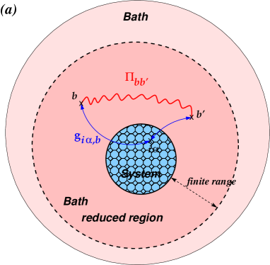
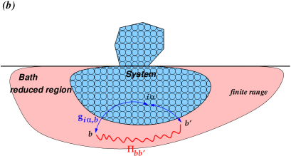
Figure 1: (Colour online) Schematic representation of total systems under consideration. This includes the finite size central system (blue) where the GLE dynamics is performed, and the bath region (pink). Because the forces $f_{b}$ and the quantities $g_{i\alpha,b}$ are of finite range (not necessarily short ranged), one can perform the mapping of $\Pi_{bb^{\prime}}(\omega)$ on a finite region of space (the bath reduced region). Furthermore, the matrix elements $\Pi_{bb^{\prime}}(\omega)$ go to zero when the distances between the two bath DOF $b$ and $b^{\prime}$ become large. The central system contains $N_{\rm at}$ atoms, the bath region $N_{B}$ atoms and the reduced bath region $N_{B}^{\rm red}$ atoms respectively.

The algorithm devised above is just one of the many possible ways of performing the mapping. Our choice clearly emphasizes a better fit for the diagonal elements $\Pi_{b,b}(\omega)$ for the mapping Eq. (13). The choice of determining the sign $\pm|c_{b}^{(k)}|$ is reminiscent of the results obtained for a finite size system, where the $c_{b}^{(k)}$ parameters would be equivalent to the components of the corresponding eigenvectors of the dynamical matrix.

Finally, one should note that since the forces $f_{b}$ and the quantities $g_{i\alpha,b}$ are of finite range (not necessarily short ranged), the Kernel built on the quantities $g_{i\alpha,b}$ and $\Pi_{b,b^{\prime}}$, see Eqs. (7) and (12), does not need to be computed by means of infinite sums on the bath indices $b$ and $b^{\prime}$. Therefore we can reduce the number of $\Pi_{b,b^{\prime}}$ components to be calculated. We perform the mapping of $\Pi_{b,b^{\prime}}(\omega)$ on a finite region of space which we call the bath reduced region as shown in Figure 1. Although this was the strategy adopted in the present study, the bath region used for the mapping and the summation in Eq. (7) with respect to the bath sites may not necessarily be the same, e.g. one may use a larger bath region for the mapping to have a better representation for the bath when fitting the parameters (and the number) of the vDOF.

IV Results for the $\bm{\Pi}(\omega)$ matrix

IV.1 Calculation of the polarisation matrix $\bm{\Pi}$

As a first step in the application of our method, we have implemented the procedure described above in the classical MD code LAMMPS Plimpton:1995 . Such a procedure is best suited to study the dissipative dynamics of the systems schematically depicted in Figure 1. These systems are typically either a bulk-like cluster (containing defects or not) coupled to its three dimensional surrounding as shown in panel (a) of Fig. 1, or any kind of structures deposited on a surface as shown in panel (b).

Once the total system is built with a clear distinction between the central system region and the bath region, we calculate the dynamical matrix using numerical differentiation of the forces acting on bath atoms obtained from LAMMPS. Note that, as mentioned previously, we consider for such calculations the whole system made of the central system and the bath region. The dynamical matrix is obtained from the conventional expression:

$$\begin{split}D_{b,b^{\prime}}=\frac{1}{\sqrt{\mu_{l}\mu_{l^{\prime}}}}\frac{\partial^{2}E_{\rm tot}}{\partial{r_{l\gamma}}\partial{r_{l^{\prime}\gamma^{\prime}}}}=\frac{1}{\sqrt{\mu_{l}\mu_{l^{\prime}}}}\frac{\partial f_{b^{\prime}}}{\partial{r_{l\gamma}}}\end{split}$$ (19)

In all our calculations, we have verified that the acoustic sum rule is fulfilled, i.e. $\sum_{b}D_{b,b^{\prime}}=\sum_{b^{\prime}}D_{b,b^{\prime}}=0$.

To validate our methodology, we show, in this paper, results for the mapping of the $\Pi_{bb^{\prime}}$ matrix and for the corresponding GLE dynamics for a simple model of a Lennard-Jones (LJ) solid. The interaction between every pair of atoms $(i,j)$ at the distance $r_{ij}$ is given by the conventional LJ potential $V(r_{ij})=4\epsilon\left[(\sigma/r_{ij})^{12}-(\sigma/r_{ij})^{6}\right]$. For convenience, we take the LJ parameters ($\epsilon=0.583$ eV and $\sigma=2.77$ Å) for a solid built as a fcc lattice with the lattice parameter $a_{0}=4.025$ Å (i.e. the nearest neighbour distance $d_{\rm NN}=\sqrt{2}/2a_{0}=2.85$ Å) [note:1, ]. In the following, we show results obtained from the dynamical matrix of the cluster made of 135 atoms (left panel in Fig. 2).

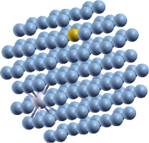
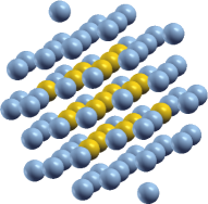
Figure 2: (Colour online) Model system of a LJ solid, fcc lattice. (Left) System for the calculation of the dynamical matrix and for the mapping. It contains the central system (made of $N_{\rm at}$ atoms) and the entire bath region (made of $N_{B}$ atoms). It has a corresponding radius of $R=7.5$ Å and $N_{B}+N_{\rm at}=135$. The bath atom labelled $l$ is coloured in yellow, and the bath atom $l^{\prime}$ is in light-grey (surrounded by interatomic bonds for clarity). (Right) System for the GLE calculations. It consists of the system region containing $N_{\rm at}=19$ atoms (yellow), and of the bath reduced region containing $N_{B}^{\rm red}=68$ atoms (grey-blue).

First we test the convergence of the calculation of $\Pi_{b,b^{\prime}}$ with respect to the number of Lanczos iterations. Figure 3 shows typical results for the diagonal matrix element $\Pi_{b,b}$ (here $b\equiv lx$ with atom $l$ shown in the left panel of Fig. 2). As expected, increasing the number of Lanczos iterations allows us to convergence towards the exact result for $\Pi_{b,b^{\prime}}$ obtained from direct diagonalisation. What is very interesting and useful for numerical applications, is that $\Pi_{b,b^{\prime}}$ can be obtained with a good level of accuracy from a number of iterations much smaller than the actual dimension $N_{\rm dim}$ of the dynamical matrix. We suspect that such a behaviour arises from the structure of the dynamical matrix, which presents the form of a sparse matrix. This is typical for a system with interaction of a finite range; however, a similar result may not hold for a system in which the interaction between atoms is dominated by long-range Coulomb interactions.

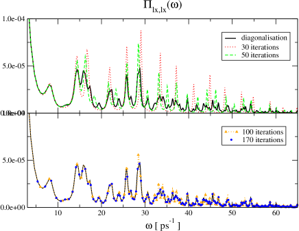
Figure 3: (Colour online) Diagonal matrix element $\Pi_{b,b}(\omega)$ for $b=lx$, with atom $l$, shown in the left panel of Fig. 2, calculated from exact diagonalisation of the dynamical matrix, and from the Lanczos iterative scheme using a different number of iterations. For this example, one gets good results after 100 iterations which is still much smaller than $N_{\rm dim}$. Calculations are performed with a small imaginary part $\varepsilon=3$. Note that, from the definition given in Eq. (30), the value of $\varepsilon$ has to be compared with the typical $\omega_{\lambda}^{2}$ values. Only the $\omega\geq 0$ part of the functions is shown here and below, since $\Pi_{b,b^{\prime}}(\omega)$ is an even function.

Figure 4 shows some typical examples for the off-diagonal matrix elements $\Pi_{b,b^{\prime}}$ obtained from converged Lanczos iterations. As expected, the off-diagonal elements have both positive and negative contributions, only the diagonal matrix elements are positive functions of $\omega$. Furthermore, each peak in the $\Pi_{b,b^{\prime}}(\omega)$ functions (as well as for the diagonal $\Pi_{b,b}(\omega)$ functions) corresponds to an eigenvalue of the dynamical matrix. Note that it does not imply that all eigenvalues are necessarily represented by peaks in any $\Pi_{b,b^{\prime}}(\omega)$ functions.

Another important point concerns the amplitude of the $\Pi_{b,b^{\prime}}(\omega)$ functions: the amplitude of the off-diagonal elements is much smaller than the amplitude of the diagonal ones (at least one order of magnitude smaller for the examples shown in Fig. 3 and Fig. 4). This is even more true when the spatial separation $d_{ll^{\prime}}$ between the two bath DOF $b$ and $b^{\prime}$ becomes larger ($d_{ll^{\prime}}\gg a_{0}$). Such a behaviour justifies a posteriori the fact that one does not need to consider all the matrix elements of an infinite bath to be able to describe properly its intrinsic vibrational properties.

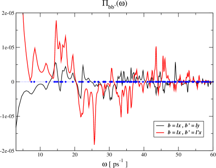
Figure 4: (Colour online) Examples of two off-diagonal matrix elements $\Pi_{b,b^{\prime}}(\omega)$ corresponding to a local (in space) matrix element $b=lx$, $b=ly$ , and a non-local matrix element $b=lx$, $b=l^{\prime}x$ where the distance between the two atoms $l$ and $l^{\prime}$ is $d_{ll^{\prime}}=2.12a_{0}=8.54$ Å. The diamond symbols represent the exact eigenvalues of the corresponding dynamical matrix. Calculations are performed with a small imaginary part $\varepsilon=3$. The two atoms corresponding to the DOF $b$ and $b^{\prime}$ are shown in the left panel of Fig. 2.

We now study the convergence properties of the $\Pi_{b,b^{\prime}}(\omega)$ versus the size of the considered bath region. This is important as increasing the size of the cluster considered in the Lanczos procedure makes more remote atoms of the bath to be available to the Lanczos iterations. For that, we consider one $\Pi_{b,b}(\omega)$ for one fixed bath index $b$ located inside the bath reduced region (see the yellow atom in the 135 atoms cluster with a radius of $R=7.5$ Å shown in the left panel of Fig. 2). We then add extra layers of atoms to this cluster to simulate a larger bath region. The convergence of the $\Pi_{b,b}(\omega)$ function is shown in Figure 5. The convergence in the lineshape of the matrix element $\Pi_{b,b}(\omega)$ is achieved for a bath region of radius $R\geq 12$ Å, which corresponds to $R\sim 3a_{0}$. These results show that the vibrational properties of the bath are more long-ranged than initially expected. We believe that the convergence does depend on the range of the pair-wise potential, which in our case is modelled with a cut-off of $R_{\rm cutoff}=6.5\sim 1.6a_{0}$.

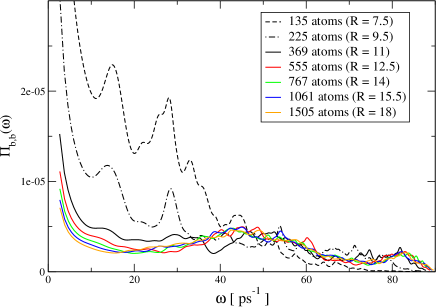
Figure 5: (Colour online) Convergence of the diagonal matrix element $\Pi_{b,b}(\omega)$ with respect to the size of the bath region. The bath DOF $b=lx$ is the yellow atom in the cluster made of 135 atoms (radius $R=7.5$ Å) as shown in the left panel of Figure 2. By adding extra layers of bath atoms, the size of the cluster increases further from 225 atoms (radius $R=9.5$ Å), 369 atoms ($R=11$ Å), 555 atoms ($R=12.5$ Å), 767 atoms ($R=14$ Å), 1061 atoms ($R=15.5$ Å) to 1505 atoms ($R=18$ Å). The convergence of the lineshape of the matrix element $\Pi_{b,b}(\omega)$ is achieved for a bath region of radius $R\geq 12$ Å. Calculations are performed with an imaginary part $\varepsilon=9$ to obtain smooth curves.

Finally, we would like to comment on the behaviour of the $\Pi_{b,b^{\prime}}(\omega)$ functions in the limit of $\omega\rightarrow 0$. The lowest frequency behaviour seems to be like $\pm 1/\omega^{a}$ (with $a\sim 1.0$). In principle, one would expect a finite value for $\Pi_{b,b}(\omega\rightarrow 0)$ as was shown analytically in Ref. [Stella et al., 2014] for a simple one-dimensional model. We argue that the behaviour at small $\omega$ we observe in our numerical simulations is due to a finite-size effect. The acoustic long-ranged vibrational properties of a solid are not appropriately well described using finite-size cluster dynamical matrix calculations. This is clear from Fig. 5 that such a behaviour becomes less and less dominant in the lineshape of $\Pi_{b,b}(\omega)$ function when the size of the system increases. The larger systems are considered, the better the description of the low-frequency, long wavelength vibrations will be.

However, we want to stress that such low frequency acoustic modes are not the vibrational modes which will be dominant in the dissipation processes between the system and the bath regions. In the following sections, we show that an approximate description of the low frequency range of the $\Pi_{b,b^{\prime}}(\omega)$ functions does not lead to the wrong physical behaviour of the dynamics of the systems obtained from the GLE, at least for not too long MD runs.

IV.2 Fitting the diagonal elements of $\Pi_{b,b}(\omega)$

Once, we have chosen the number of vDOF we want to work with, the fitting procedure described in Sec. III.2 is used to map the diagonal elements $\Pi_{b,b}(\omega)$ according to the expression given in Eq. (13).

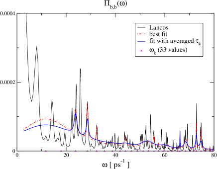
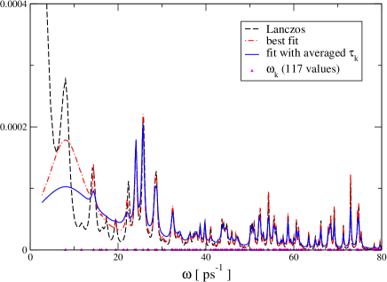
Figure 6: (Colour online) Typical example for the fit of a diagonal element of $\Pi_{b,b}(\omega)$ performed by using 33 different values for the vDOF peak positions $\omega_{k}$ (top panel) and 117 values for $\omega_{k}$ (bottom panel). As one would expect for any fitting procedure, the more elementary functions are put in the fit, here Lorentzian of width $1/\tau_{k}$ and position $\omega_{k}$, the better the fit is.

We chose to consider below the $\Pi_{b,b}(\omega)$ functions which present a lot of peaks, as opposed to low features functions obtained with a large bath region (see Fig. 5). We do this in order to test the robustness of our fitting procedure.

Figure 6 shows a typical example of our mapping procedure for a diagonal element of $\Pi_{b,b}(\omega)$. The best fit is given by the red curves. After fitting all the diagonal elements $\Pi_{b,b}(\omega)$, we calculated (as explained in Sec. III.2) an effective $\tau_{k}$ value associated with each peak at $\omega_{k}$, as the extended Langevin dynamics deals with $\{\tau_{k},\omega_{k}\}$ parameters independent of the bath index $b$. Using the smallest of all $\tau_{k}$ (for each peak at $\omega_{k}$), we still obtain a good fit (blue curves) of the original $\Pi_{b,b}(\omega)$ result.

Note that as expected for any fitting procedure, the more elementary functions (Lorentzian of width $1/\tau_{k}$ and position $\omega_{k}$) are used for the mapping, the better the fit is. However, we show below that both sets of fitting parameters will lead to a proper physical behaviour of the system, i.e. as far as the thermalisation of the kinetic energy and velocity distributions are concerned.

IV.3 Fitting the off-diagonal elements of $\Pi_{b,b^{\prime}}(\omega)$

As explained in Sec. III.2, once the parameters $\tau_{k}$ and $|c_{b}^{(k)}|$ are obtained from the fits of the diagonal elements $\Pi_{b,b}(\omega)$, the proper sign of all the coefficients $c_{b}^{(k)}$ is determined from the best fit of the off-diagonal elements $\Pi_{b,b^{\prime}}(\omega)$. A typical best fit result is shown in Figure 7.

With such a procedure, we obtain an approximate fit of the $\Pi_{b,b^{\prime}}(\omega)$ function, which is not as good as for the diagonal elements. However, in some ranges of frequency, the off-diagonal matrix elements are very well reproduced by our mapping scheme as shown in Figure 7.

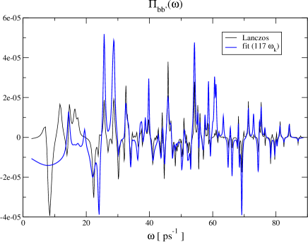
Figure 7: (Colour online) Typical example for the fit of an off-diagonal element of $\Pi_{b,b^{\prime}}(\omega)$. Fit is performed by using 117 different values for the vDOF peak position $\omega_{k}$.

We would like to stress again that the fitting scheme of all $\Pi_{b,b^{\prime}}(\omega)$ functions is a highly non-trivial multi-variable optimisation problem, which includes strong constraints (i.e. the parameters $\{\tau_{k},\omega_{k}\}$ are independent of the bath indexes $b,b^{\prime}$). In this paper, we have provided one possible scheme to perform such a mapping, but many more are available. We are currently investigating other routes SummerStudents:2014 .

V Results for the GLE in the extended phase space

V.1 Thermalisation of the system

First of all, we study how the system thermalises in our model of a realistic bath characterised by a set of parameters $\{\tau_{k},\omega_{k},c_{b}^{(k)}\}$. Initially, the atomic positions in the central system are at equilibrium and all velocities are set to zero. We then run different extended GLE dynamics simulations using the algorithm described in detail in Appendix B.

We want to stress that all the dynamics we have obtained, for the different sets of parameters $\{\tau_{k},\omega_{k},c_{b}^{(k)}\}$, are stable. We do not obtain any pathological behaviour in the calculations of the atomic positions and velocities over thousands of time steps (runs of up to 80 ps using a time step of $\Delta t=1$ fs). In the following, we present a few selected results from all the calculations we have performed.

Figures 8 and 9 represent the evolution of the total kinetic energy for the system shown in the right panel of Fig. 2. The system on which the GLE is performed contains $N_{\rm at}=19$ atoms, and the bath reduced region contains 68 atoms. The mapping of the $\Pi_{bb^{\prime}}(\omega)$ functions is performed by using 33 vDOF (see Fig. 8) and 117 vDOF (see Fig. 9). We recall that during the mapping procedure, the dynamical matrix is obtained for a bath region of radius $R=7.5$ Å which contains 135 atoms (see left panel of Fig. 2).

The results of our GLE calculations show that the system thermalises towards the proper equilibrium temperature as expected, since the averaged total kinetic energy follows the equipartition principle and oscillates around the expected value of $E_{\rm kin}^{\rm TOT}=3/2N_{\rm at}k_{B}T$. Such a behaviour is obtained for all the temperatures $T=100,300,600,800$ K we have considered and for different sets of fitting parameters. The time taken by the system to reach the thermal equilibrium depends strongly on the values of the fitting parameters, more specifically on the relaxation times $\{\tau_{k}\}$ associated with the vDOF.

Further examples for the thermalisation of the system are provided in Appendix C.

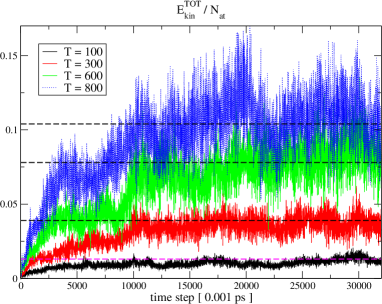
Figure 8: (Colour online) Total kinetic energy of the system region containing 19 atoms shown in the right panel of Fig. 2. The GLE calculations are performed for different bath temperatures $T$ (in K) and for a set of fitting parameters obtained with 33 vDOF, and for the bath region of radius $R=7.5$ Å (135 atoms), see Fig. 6. The system thermalises to the proper equilibrium temperature after $t\sim 15-18$ ps. The horizontal lines correspond to the different values of $3/2k_{B}T$ and show that the GLE dynamics properly equilibrates the system region according to the equipartition principle. The energies are given in [eV].

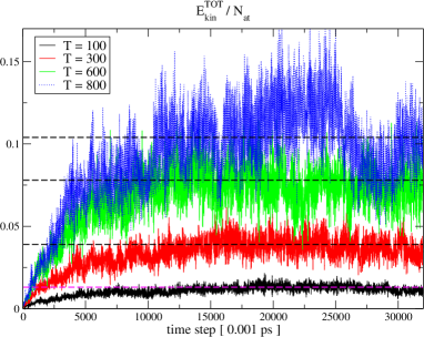
Figure 9: (Colour online) Total kinetic energy of the system region containing 19 atoms shown in the right panel of Fig. 2. The GLE calculations are performed for different bath temperatures $T$ (in K) and for the set of fitting parameters obtained with 117 vDOF (see Fig. 6 and Fig. 7). The results are quantitatively different from the calculations performed with 33 vDOF (Fig. 8), but are qualitatively similar. The system thermalises, as expected, to the proper equilibrium temperature after a shorter time $t\sim 12-15$ ps in comparison with Fig. 8.

V.2 Velocity distributions

From the time evolution of the total kinetic energy, we can extract an effective velocity $v_{\rm eff}$ from the relation $1/2mv_{\rm eff}^{2}=E_{\rm kin}^{\rm TOT}/N_{\rm at}$. Using the time series of such a velocity, we can build up a histogram of the velocity in a range of the time span $[t_{1},t_{2}]$ for which the system is thermalised. Figure 10 represents such a histogram for different temperatures, using the values of the total kinetic energy shown in Fig. 9 and for the range $[t_{1},t_{2}]=[20,32]$ ps.

We have checked that the full width at half maximum (FWHM) follows the behaviour of a Gaussian distribution in $e^{-\beta mv_{\rm eff}^{2}/2}$, i.e. the ratio between two FWHMs for two different temperatures is like $\Delta v_{\rm eff}(T_{1})/\Delta v_{\rm eff}(T_{2})=\sqrt{T_{1}/T_{2}}$. In other words, such a result can be understood as follows: the system thermalises to the expected bath temperature, and the corresponding effective temperature fluctuates around the mean value according to a Gaussian distribution.

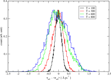
Figure 10: (Colour online) Histograms of the effective velocity built from the time series of the kinetic energy shown in Fig. 9. The histograms are centred around the corresponding mean effective velocity $\langle v_{\rm eff}\rangle$. The widths of the distributions follow a Gaussian distribution in $\exp(-\beta mv_{\rm eff}^{2}/2)$.

More importantly, we can also study the statistics of the velocity of individual atoms in the central region. For that, we build the velocity distribution $P_{v}(t_{i})$ of the velocities $v_{i}=(\sum_{\alpha=x,y,z}v_{i\alpha}^{2})^{1/2}$ of each individual atom $i$ in the central region for the set of velocities obtained at time $t_{i}$ when the system is thermalised. In order to obtain a better statistical representation of such a distribution, we calculate an averaged distribution

$$\bar{P}_{v}=\sum_{i=1}^{N_{\rm ts}}P_{v}(t_{i})/N_{\rm ts}$$ (20)

over a set of $N_{\rm ts}$ different times $t_{i}$ in the time range $[t_{1},t_{2}]$ for which the system is thermalised.

An example of the velocity distribution $\bar{P}_{v}$ is shown in Figure 11. The GLE calculations were performed by using the set of parameters $\{\tau_{k},\omega_{k},c_{b}^{(k)}\}$ based on 117 vDOF. In the calculation of $\bar{P}_{v}$, we used $N_{\rm ts}$=220 different time steps $t_{i}$ equally spaced in the time range $t=[30,52]$ ps. We also compared the calculated distribution $\bar{P}_{v}$ with the corresponding Maxwell-Boltzmann distribution defined as

$$f_{v}=\sqrt{\left(\frac{m\beta}{2\pi}\right)^{3}}4\pi v^{2}e^{-mv^{2}/2\beta}.$$ (21)

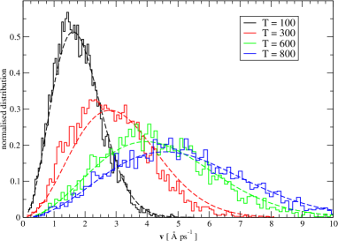
Figure 11: (Colour online) Histograms of the velocity distribution $\bar{P}_{v}$ calculated from a GLE dynamics based on the use of 117 vDOF. $\bar{P}_{v}$ is obtained from $N_{\rm ts}$=220 different timesteps $t_{i}$ taken in the range $t=[30,52]$ ps. The broken curves correspond to the Maxwell-Botzmann distribution $f_{v}$ and represent an almost perfect fit between the two velocity distributions.

From Figure 11, we can see an almost perfect match between the two distributions $\bar{P}_{v}$ and $f_{v}$.

To conclude this section, we can confidently say that our extended GLE calculations provide a good thermostat model, in the sense that the central system thermalises towards the expected temperature, with expected Gaussian fluctuations around the mean value of the effective temperature. More importantly, the thermostat provides the correct canonical distribution of the velocities in the central region once the system is thermalised.

V.3 Velocity autocorrelation functions

One last dynamical quantity that we need to examine is the velocity autocorrelation functions of the central system. The velocity autocorrelation functions (VACF) are calculated from

$$\langle v(t_{0})v(t+t_{0})\rangle=\sum_{i\alpha}v_{i\alpha}(t_{0})v_{i\alpha}(t+t_{0})/(3N_{\rm at})$$ (22)

for all atoms $i$ of the central region and with $t>t_{0}$.

For the two times $t_{0}$ and $t$ being within the time range where the system is thermalised, the VACF should be dependent only on the time argument difference $\Delta t=(t+t_{0})-t_{0}$, i.e. independent of the initial time $t_{0}$. In order to obtain a better statistical representation of the VACF, we also calculate an averaged VACF from different $N_{\rm samp}$ samplings of the initial time $t_{0}$ in a time range where the system is thermalised:

$$\overline{\langle v(0)v(t)\rangle}=\sum_{\{t_{0}\}}^{N_{\rm samp}}\langle v(t_{0})v(t+t_{0})\rangle/N_{\rm samp}.$$ (23)

Figure 12 represents the corresponding averaged velocity autocorrelation functions $\overline{\langle v(0)v(t)\rangle}$ for the central system containing 19 atoms shown in Fig. 2 and for the temperature $T=100$ K. The GLE calculations were performed with the set of fitting parameters based on 117 vDOF. The averaged VACF was calculated for $t_{0}\sim 40$ ps and $t\sim 40.5$ ps and using 300 different samplings of the initial time $t_{0}$ over the time range $\sim[40,41.5]$ ps. Our GLE results show the proper decaying behaviour of the VACF with the time difference $\Delta t$. It is interesting to note that the loss of the velocity correlation occurs on a much shorter time scale than the time scale corresponding to the thermalisation of the system (starting from zero velocities).

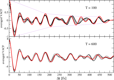
Figure 12: (Colour online) Velocity autocorrelation functions for the central system region containing 19 atoms. Calculations for the averaged VACF $\overline{\langle v(0)v(t)\rangle}$ are obtained with the set of fitting parameters corresponding to Fig. 9 and for two temperatures $T=100$ K (top panel) and $T=600$ K (bottom panel). The average is obtained from 300 different samplings of the initial time $t_{0}$ over the time range $[40,41.5]$ ps. The different thin lines correspond to different sets of sampling. The dotted lines in the upper panel are a guide for the eye to show the decaying of the VACF with the time difference $\Delta t$.

V.4 Simplified Langevin dynamics with a single friction coefficient

To further confirm the validity of our approach, we now compare our GLE results with the more conventional approach of the Langevin dynamics, using a more heuristic description of the dissipation in the system:

$$\begin{split}\dot{\mathbf{p}}=-\mathbf{\nabla}_{\mathbf{r}}\bar{V}(\mathbf{r})-\gamma\mathbf{p}+\bm{\xi}_{G}\end{split}$$ (24)

with the momentum vector $\mathbf{p}=\mathbf{M}\dot{\mathbf{r}}$ and the random noise vector $\bm{\xi}_{G}$. The latter follows a Gaussian distribution Uhlenbeck:1930 ; Gillespie:1996 . The random noise has the dispersion which is related directly to the friction coefficient via the well-known expression $\sigma_{i}^{2}=2M_{i}\gamma k_{B}T/\Delta t$, where $\Delta t$ is the time step of the dynamics. Note that the friction and random forces are applied here to all the atoms of the central system. The Gaussian Langevin dynamics has already been implemented in the code LAMMPS Toton:2010 ; Plimpton:1995 .

Figure 13 shows the time evolution of the total kinetic energy of the system region containing 19 atoms (right panel of Fig. 2). Both GLE and conventional Langevin dynamics provide a total kinetic energy that converges towards the expected thermodynamical equilibrium value of $3/2N_{\rm at}k_{B}T$ (with $T=100$ K). One can see that the conventional Langevin dynamics results can fit fairly well the results obtained from the GLE calculations by adjusting the friction coefficient $\gamma$. For the target temperature of the bath $T=100$ K and the initial temperature $T_{\rm init}=0$ (initially, all velocities are set to zero), we obtain the best correspondence between the conventional Langevin dynamics and the GLE dynamics for the friction constant value $\gamma=1/\tau_{\rm damp}$ with $\tau_{\rm damp}\sim 9.0-9.5$ ps.

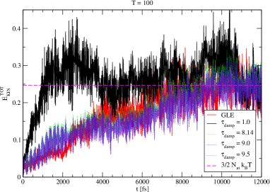
Figure 13: (Colour online) Total kinetic energy of the system region containing 19 atoms shown in the right panel of Fig. 2. The plots show a comparison between GLE calculations and conventional Langevin dynamics with a simple friction constant $\gamma$ for bath temperature of $T=100$ K. All total kinetic energies converge towards the expected thermodynamical equilibrium value. One obtains a good correspondence between the conventional Langevin dynamics and the GLE dynamics for a friction constant $\gamma=1/\tau_{\rm damp}$, with $\tau_{\rm damp}\sim 9.0-9.5$ ps. Initially, all velocities are set to zero.

Such a range of values for the friction constant of the conventional Langevin dynamics seems to provide the appropriate behaviour of the total kinetic energy for the model bath we have used. We have checked that the range $\tau_{\rm damp}\sim 9.0-9.5$ ps provides the appropriate behaviour of $E_{\rm kin}^{\rm TOT}$ when the dynamics are started with initial velocities different from zero. Furthermore, we have also checked that such a range of $\tau_{\rm damp}$ is appropriate for a range of temperatures going from $T=100$ to $T=600$ K.

Finally we can compare the VACF obtained from the conventional Langevin dynamics with our GLE calculations. Figure 14 shows the averaged VACF for one temperature. The averages of the VACF are performed in exactly the same way for all the calculations. We can observe a good correspondence between the GLE and conventional Langevin calculations. The loss of correlation in the velocities appears slightly earlier for the GLE calculations. The dependence of the VACF upon the friction constant seems weaker than for the kinetic energy, however the best correspondences are obtained for the range of damping $\tau_{\rm damp}\sim 9.0-9.5$ ps.

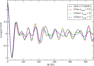
Figure 14: (Colour online) Velocity autocorrelation functions for the central system region containing 19 atoms. The plots show the averaged VACF $\overline{\langle v(0)v(t)\rangle}$ for a temperature $T=100$ K for the GLE runs based on 117 vDOF and for the conventional Langevin dynamics (LGauss) with different friction constants $\gamma=1/\tau_{\rm damp}$. The average is obtained from 600 different samplings of the initial time $t_{0}$ over the time range $[48.5,49.0]$ ps. All averaged VACF are performed in exactly the same manner.

It should be noted that, for the present model of a homogeneous LJ solid used in our calculations, the results obtained with the conventional Langevin dynamics are indeed very similar to the results obtained with our more general and complex GLE method. However, there is one fundamental difference between the two approaches: the conventional Langevin dynamics requires an a priori unknown input parameter, i.e. the friction constant $\gamma$, which is not the case for our GLE approach. As shown above, our GLE approach can be used to extract such an input parameter for the heuristic Langevin equation.

VI Summary and Discussion

In this paper, we have implemented the GLE scheme developed in Refs. [Kantorovich:2008, ] and [Stella et al., 2014] and have shown several applications for systems described at the atomic level. We recall that this GLE scheme goes beyond a bi-linear coupling between the central system and the bath, and permits us to have a realistic description (i.e. at the atomic level) of both the dissipative central system and its surrounding bath. This implementation of the GLE scheme is done in the classical MD code LAMMPS.

We have shown how to obtain the vibrational properties of a realistic bath and how to convey such properties into an extended Langevin dynamics by the use of the mapping of the bath vibrational properties onto a set of auxiliary DOF, see Eq. (13).

Different applications of such a mapping scheme and of the corresponding extended Langevin dynamics were given for different models of a LJ solid. In this manuscript, the implementation of our GLE method is done for pair-wise interatomic potential. The use of such potentials makes the calculations of the different quantities, such as $f_{b}(\{r_{i\alpha}\})$ and $g_{i\alpha,b}(\{r_{i\alpha}\})$ to be evaluated twice at each time step, much faster. Implementation for any type of N-body potential is under consideration.

All our calculations show that our GLE scheme provide a stable Langevin dynamics, with the dissipative/relaxation processes properly described. The total kinetic energy of the central system always thermalises toward the expected bath temperature, with appropriate fluctuation around the mean value. More importantly, we obtain a velocity distribution for the individual atoms in the central system which follows the expected canonical distribution at the corresponding temperature. This confirms that both our GLE scheme and our mapping procedure onto an extended Langevin dynamics provide the correct thermostat. We have also examined the corresponding VACF and found that the velocities lose correlations as expected, however the corresponding time scale is much shorter than the time taken by the system to reach thermalization.

We have also compared our GLE results with respect to more conventional Langevin dynamics based on a single relaxation time (i.e. single friction coefficient). Our calculations have shown the possibility of extracting an effective friction coefficient from our realistic bath model, which then could be used a posteriori in a much less expensive Langevin dynamics. Our calcutations have shown that the obtained effective friction coefficient is independent on the initial distribution of the velocities and on the temperature of the system (at least for the range 100—600 K we have considered).

One has to have in mind, however, that it is only for the rather simple model system considered here that the friction coefficient of the heuristic Langevin dynamics was found to be temperature independent. There is no reason to believe that this is a general rule and that for other systems, e.g. highly inhomogeneous, it will still be the case. Furthermore, in the cases of heterogeneous systems different values of the friction coefficient for different species need to be found. It is not clear a priori what value is to be used, and also how the right value can be chosen in practice. Indeed, as was shown in Ref.[Kantorovich:2008b, ], any value of the friction coefficient, even if applied not to all atoms of the system, would always bring the system to the equilibrium state described by the corresponding canonical distribution. Hence the value of the friction parameter(s) can only be obtained by running genuinely non-equilibrium simulations, e.g. on heat transport, rate of equilibration and so on. It seems that using GLE eliminates all these problems by providing a clear and fundamentally sound platform for either running (more expensive) GLE type calculations or using GLE for fitting the value(s) of the friction coefficient(s). If necessary, temperature dependent friction is also within reach.

Finally, we would like to comment on two different points. First, the results presented in this paper were obtained for a homogeneous “rather simple” system (i.e. made of only one chemical species), furthermore the system does not have a complicated geometry. Our GLE scheme is however applicable to much more complex systems (i.e. highly heterogeneous, and with complex structures like bio-like molecules deposited on rough surfaces). The results presented in this paper should be mostly understood as a proof of principle of our methodology.

For complex systems, we expect that the bath vibrational properties will present more specific features which will lead to more specific properties of the memory kernel. In turn, the properties of such a kernel will strongly affect, by some kind of selective processes, the efficiency of some vibrational modes of the central region to exchange energy with the surrounding bath. We expect that such specific bath properties will be central in the thermalization and relaxation processes of (small to large) molecules grafted onto surfaces or clusters (and into the presence or not of solvents).

Second, a large number of equilibrium thermostats has been designed up to date (see Refs. [Toton:2010, ] and references therein). The GLE can be used to provide exactly the same results as obtained from these equilibrium thermostates, albeit with a higher computational cost. However, the main advantage of the GLE, as compared with the other available equilibrium thermostats, is that it is also applicable to the study of nonequilibrium processes. For instance, the GLE technique is, by essence, naturally applicable for studying the phonon contribution to thermal transport through bulk materials or nano-junctions. Such nonequilibrium processes can be treated by coupling the central system to more than one bath. Each bath would be at its own equilibrium, and one cannot define a single temperature for the whole system. In that case, the central system does not evolve towards an equilibrium state, but will eventually reach a steady state regime characterised by heat flows between the central system and the baths. To study such processes, the GLE equation (9) can be generalised to include the nonequilibrium conditions when the different baths are independent (i.e. not coupled to each other in any way). For that we simply need to extend the number of virtual DOF to obtain a set of parameters $\{\tau_{k},\omega_{k},c_{b}^{(k)}\}_{\nu}$ for each bath $\nu$ at temperature $T_{\nu}$. Each bath $\nu$ will also be characterised by its own dynamical matrix and matrix elements ${\Pi}_{b,b^{\prime}}^{\nu}$. The implementation of such nonequilibrium extended Langevin dynamics is currently under development.

Appendix A Bath vibration propagator and $\bm{\Pi}$ matrix

In Ref. [Kantorovich:2008, ] it is shown that, in the time representation, the matrix $\bm{\Pi}(t-t^{\prime})$ is related to the bath propagator $\bm{\mathcal{D}}(t-t^{\prime})$ via $\partial_{\tau}\bm{\Pi}(\tau)=-\bm{\mathcal{D}}(\tau)$.

The bath propagator $\bm{\mathcal{D}}(t-t^{\prime})$ is the solution of the harmonic dynamics of the bath DOF

$$\sum_{b_{1}}\left[\partial_{t}^{2}+D_{b,b_{1}}\right]\mathcal{D}_{b_{1},b^{\prime}}(t-t^{\prime})=\delta(t-t^{\prime})\delta_{b,b^{\prime}},$$ (25)

where $[\bm{D}]_{b,b^{\prime}}$ are the elements of the dynamical matrix of the bath region.

The elements of the matrix $\bm{\Pi}$ are given by Kantorovich:2008

$${\Pi}_{b,b^{\prime}}(t-t^{\prime})=\sum_{\lambda}e_{\lambda}^{b{\dagger}}e_{\lambda}^{b^{\prime}}\ \frac{\cos\omega_{\lambda}(t-t^{\prime})}{\omega_{\lambda}^{2}}$$ (26)

where $\lambda$ labels the eigenstates of the dynamical matrix $\bm{D}$ with eigenvalues $\omega_{\lambda}^{2}$ and eigenvectors $\bm{e}_{\lambda}$ with component $e_{\lambda}^{b}$ in the bath region.

As all quantities depend only on a single time argument, one can pass into the energy representation after using the Fourier transform.

The bath propagator $\mathcal{D}(\omega)$ is then the solution of

$$\sum_{b_{1}}[(i\omega)^{2}\bm{1}+\bm{D}]_{b,b_{1}}\mathcal{D}_{b_{1},b^{\prime}}(\omega)=\delta_{b,b^{\prime}}$$ (27)

and

$$\begin{split}{\Pi}_{b,b^{\prime}}(\omega)&=\sum_{\lambda}e_{\lambda}^{b{\dagger}}e_{\lambda}^{b^{\prime}}\ \frac{1}{\omega_{\lambda}^{2}}\left(\delta(\omega-\omega_{\lambda})+\delta(\omega+\omega_{\lambda})\right)\frac{2\pi}{2}\\ &=\sum_{\lambda}e_{\lambda}^{b{\dagger}}e_{\lambda}^{b^{\prime}}\ \frac{2\pi}{|\omega_{\lambda}|}\delta(\omega^{2}-\omega_{\lambda}^{2})\\ &=\frac{2\pi}{|\omega|}\sum_{\lambda}e_{\lambda}^{b{\dagger}}e_{\lambda}^{b^{\prime}}\ \delta(\omega^{2}-\omega_{\lambda}^{2}).\end{split}$$ (28)

It is now easy to find the relationship between $\bm{\Pi}(\omega)$ and $\bm{\mathcal{D}}(\omega)$:

$${\Pi}_{b,b^{\prime}}(\omega)=-\frac{2}{|\omega|}{\rm Im}\left[\omega^{2}\bm{1}-\bm{D}+i\varepsilon\right]^{-1}_{b,b^{\prime}},$$ (29)

by introducing a small imaginary part in

$$\mathcal{D}_{b,b^{\prime}}(\omega)=-\sum_{\lambda}e_{\lambda}^{b{\dagger}}e_{\lambda}^{b^{\prime}}\ (\omega^{2}-\omega_{\lambda}^{2}+i\varepsilon)^{-1}$$ (30)

and using the fact that $i\omega\bm{\Pi}(\omega)=-\bm{\mathcal{D}}(\omega)$.

Appendix B Verlet-type algorithm for the extended Langevin dynamics

Following the prescriptions given in Ref. [Stella et al., 2014], we use the following algorithm for a single time-step $\Delta t$. The algorithm is derived, in a Verlet-style, from a different splitting and a Trotter-like decomposition of the total Liouvillian for the extended Langevin dynamics of the system DOF, $r_{i\alpha}$, and the virtual DOF $s_{1,2}^{(k)}$. Such a decomposition has been shown to provide a more appropriate description of the velocity correlation functions Leimkuhler:2013 .

Algorithm:

$$\begin{split}&\text{(A) Randomise and propagate the vDOF}\\ &s_{x}^{(k)}\leftarrow a_{k}s_{x}^{(k)}+b_{k}\xi_{x}^{(k)}\\ &\text{(B) Calculate all $f_{b}(\{r_{i\alpha}\})$ and $g_{i\alpha,b}(\{r_{i\alpha}\})$}\\ &\text{(C) Propagate the DOF and vDOF}\\ &v_{i\alpha}\leftarrow v_{i\alpha}+\left(f_{i\alpha}+f_{i\alpha}^{\rm pol}+f_{i\alpha}^{p{\rm GLE}}\right)\frac{\Delta t}{2m_{i}}\\ &s_{2}^{(k)}\leftarrow s_{2}^{(k)}-\omega_{k}s_{1}^{(k)}\frac{\Delta t}{2}\\ &r_{i\alpha}\leftarrow r_{i\alpha}+v_{i\alpha}\Delta t\\ &\text{(D) Recalculate all $f_{b}(\{r_{i\alpha}\})$ and $g_{i\alpha,b}(\{r_{i\alpha}\})$}\\ &\text{(E) Propagate the DOF and vDOF}\\ &s_{1}^{(k)}\leftarrow s_{1}^{(k)}+\left(\omega_{k}s_{2}^{(k)}+f_{k}^{s{\rm GLE}}\right)\Delta t\\ &v_{i\alpha}\leftarrow v_{i\alpha}+\left(f_{i\alpha}+f_{i\alpha}^{\rm pol}+f_{i\alpha}^{p{\rm GLE}}\right)\frac{\Delta t}{2m_{i}}\\ &s_{2}^{(k)}\leftarrow s_{2}^{(k)}-\omega_{k}s_{1}^{(k)}\frac{\Delta t}{2}\\ &\text{(F) Randomise and propagate the vDOF}\\ &s_{x}^{(k)}\leftarrow a_{k}s_{x}^{(k)}+b_{k}\xi_{x}^{(k)}\end{split}$$ (31)

where the different forces, $f_{i\alpha},f_{i\alpha}^{\rm pol},f_{i\alpha}^{p{\rm GLE}},f_{k}^{s{\rm GLE}}$ are explained below. The force

$$f_{i\alpha}=-\frac{\partial{V}(\mathbf{r})}{\partial r_{i\alpha}}$$ (32)

is the force acting on the system DOF ${i\alpha}$ due to the interaction between the atoms in the system and in the bath region(s); the “polaronic” force $f_{i\alpha}^{\rm pol}$

$$\begin{split}f_{i\alpha}^{\rm pol}&=\sum_{b,b^{\prime}}\sqrt{\mu_{l}\mu_{l^{\prime}}}\ g_{i\alpha,b}\ \Pi_{bb^{\prime}}(0)f_{b^{\prime}}\\ &=\sum_{b,b^{\prime},k}\sqrt{\mu_{l}\mu_{l^{\prime}}}\ g_{i\alpha,b}(\{r_{i\alpha}\})\ c_{b}^{(k)}c_{b^{\prime}}^{(k)}\ f_{b^{\prime}}(\{r_{i\alpha}\})\end{split}$$ (33)

(with $b\equiv l\gamma$ for the bath DOF) is the force acting on the system DOF ${i\alpha}$ due to the interaction between the system and bath regions which induces a displacement of the positions of the harmonic oscillators characterising the bath. In Eq. (33), we used the fact that $\Pi_{bb^{\prime}}(0)$ is the inverse Fourier transform (evaluated at $\tau=0$) of $\Pi_{bb^{\prime}}(\omega)$ given by Eq. (13).

The force $f_{i\alpha}^{p{\rm GLE}}$ acts on the system DOF ${i\alpha}$ and arises from the generalised Langevin equations:

$$f_{i\alpha}^{p{\rm GLE}}=\sum_{b,k}\sqrt{\frac{\mu_{l}}{\bar{\mu}}}\ g_{i\alpha,b}(\{r_{i\alpha}\})\ c_{b}^{(k)}s_{1}^{(k)}$$ (34)

and the force $f^{s{\rm GLE}}$ acts on the vDOF $s_{1}^{(k)}$ and also arises from the generalised Langevin equations

$$f_{k}^{s{\rm GLE}}=-\sum_{i\alpha,b}\sqrt{\mu_{l}\bar{\mu}}\ g_{i\alpha,b}(\{r_{i\alpha}\})\ c_{b}^{(k)}v_{i\alpha}$$ (35)

The integration of the dissipative part of the dynamics of the vDOF (see steps (A) and (F) in the algorithm) includes the coefficients $a_{k}={\rm exp}(-\Delta t/2\tau_{k})$ and $b_{k}=[k_{B}T\bar{\mu}(1-a_{k}^{2})]^{1/2}$ and the uncorrelated random variable $\xi_{1,2}^{(k)}$ corresponding to the white noise.

Appendix C Further examples for the system thermalisation

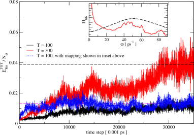
Figure 15: (Colour online) Total kinetic energy of the system region containing 19 atoms shown in the right panel of Fig. 2. The GLE calculations are performed for different bath temperatures $T$ (in K) and for the set of fitting parameters obtained with 48 vDOF, and for a larger bath region of radius $R=12.5$ Å (555 atoms) (see a corresponding $\Pi_{b,b}$ function given by the red curve in Fig. 5). The system thermalises, as expected, to the proper equilibrium temperature after a time $t\sim 30$ ps. The inset represents a poor fitting of the $\Pi_{bb^{\prime}}$ functions with 27 vDOF, with the dashed curve representing the fit and the red curve the exact result. The corresponding GLE calculations for the total kinetic energy (blue broken line) are shown for $T=100$. The system thermalises much faster because the corresponding values of the $\tau_{k}$ parameters are much smaller than for the fit using 48 vDOF.

Figure 15 shows another example of the time evolution of the total kinetic energy of the central system. For these calculations, the set of parameters $\{\tau_{k},\omega_{k},c_{b}^{(k)}\}$ corresponds to 48 vDOF, and the mapping is performed for the larger bath region of radius $R=12.5$ Å (555 atoms) (for an example of the corresponding $\Pi_{bb}$ functions see the red curve in Fig. 5). Once more, we can observe the thermalization of the system towards the expected equilibrium thermodynamical values for the two different temperatures. However the overall dynamics is slower than in the previous two cases. Such a behaviour depends on the values of the parameters $\{\tau_{k},\omega_{k},c_{b}^{(k)}\}$ obtained from the mapping.

We would like to mention that we can perform an analysis of the temporal evolution of kinetic energy in terms of the values of the relaxation times. Such an analysis is approximate, but still good enough when the spreading of the different values of the parameters $\tau_{k}$, for a given fit, is not too large. In such a case, all $\tau_{k}$ values are almost the same. For the example of a poor fit shown in the inset of Fig. 15, we have $\tau_{k}\sim 0.05$ ps for all the 27 vDOF. The corresponding total kinetic energy (blue curve in Fig. 15) approaches the thermal equilibrium value more quickly than for the mapping obtained with 48 vDOF. Indeed, for the mapping done with 48 vDOF, we have $\tau_{k}$ parameters with more spread values and an averaged relaxation time is around 2-3 ps which is much larger than $\sim 0.05$ ps and explains why the system (described with the 48 vDOF) thermalises on a longer time-scale than the system described by a poor fit with 27 DOF.

For the results presented in Fig. 8 and Fig. 9, the distribution of the values of the parameters $\tau_{k}$ is substantially broader with values ranging from $\tau_{k}\sim 0.06$ to $\sim 6$ ps for the mapping made with 117 vDOF, and from $\sim 0.06$ to $\sim 14$ ps for the mapping made with 33 vDOF. Correspondingly, the time taken by the system to thermalize is intermediate between the thermalization times shown in Figure 15.

References

- (1)
- (2) S. Berber, Y.-K. Kwon, and D. Tománek, Phys. Rev. Lett. 84, 4613 (2000)
- (3) P. Kim, L. Shi, A. Majumdar, and P. L. McEuen, Phys. Rev. Lett. 87, 215502 (2001)
- (4) L. Shi and A. Majumdar, J. Heat Trans. - T. ASME 124, 329 (2002)
- (5) C. W. Padgett and D. W. Brenner, Nano Letters 4, 1051 (2004)
- (6) M. Hu, P. Keblinski, J.-S. Wang, and N. Raravikar, Journal of Applied Physics 104, 083503 (2008)
- (7) C. W. Padgett, O. Shenderova, and D. W. Brenner, Nano Lett. 6, 1827 (2006).
- (8) N. Yang, G. Zhang, and B. Li, Nano Lett. 8, 276 (2008).
- (9) S. K. Estreicher and T. M. Gibbons, Physica B 404, 4509 (2009).
- (10) D. Segal and A. Nitzan, J. Chem. Phys. 117, 3915 (2002).
- (11) N. Mingo and Liu Yang, Phys. Rev. B 68, 245406 (2003).
- (12) Z. Yao, J.-S. Wang, B. Li and G.-R. Liu, Phys. Rev. B 71, 085417 (2005).
- (13) J.-S. Wang, Phys. Rev. Lett. 99, 160601 (2007).
- (14) Y. Dubi and M. Di Ventra, Rev. Mod. Phys. 83, 131 (2011).
- (15) J. R. Widawsky, P. Darancet, J. B. Neaton, and L. Venkataraman, Nano Lett. 12, 354 (2012).
- (16) D. G. Cahill, K. Goodson, and A. Majumdar, J. Heat Trans. - T. ASME 124, 223 (2002)
- (17) E. Pop, Nano. Res. 3, 147 (2010)
- (18) M. Zebarjadi, K. Esfarjani, M. S. Dresselhaus, Z. F. Ren, and G. Chen, Energy Environ. Sci. 5, 5147 (2012)
- (19) H. Mori, Prog. Theor. Phys. 33, 423 (1965).
- (20) S. A. Adelman and J. Doll, J. Chem. Phys. 64, 2375 (1976).
- (21) S. A. Adelman, J. Chem. Phys. 73, 3145 (1980).
- (22) D. L. Ermak and H. Buckholz, J. Comp. Phys. 35, 169 (1980).
- (23) B. Carmeli and A. Nitzan, Chem. Phys. Lett. 102, 517 (1983).
- (24) E. Cortés, B. J. West and K. Lindenberg, J. Chem. Phys. 82, 2708 (1985).
- (25) R. Tsekov and E. Ruckenstein, J. Chem. Phys. 100, 1450 (1994).
- (26) R. Tsekov and E. Ruckenstein, J. Chem. Phys. 101, 7844 (1994).
- (27) H. Risken, The Fokker-Planck Equation: Methods of Solutions and Applications, 2nd ed. (Springer, Berlin, 1996).
- (28) R. Hernandez, J. Chem. Phys. 111, 7701 (1999).
- (29) R. Zwanzig, Nonequilibrium Statistical Mechanics (Oxford University Press, 2001)
- (30) D. Segal, A. Nitzan and P. Hänggi, J. Chem. Phys. 119, 6840 (2003).
- (31) R. Kupferman, J. Stat. Phys. 114, 291 (2004).
- (32) J.-D. Bao, J. Stat. Phys. 114, 503 (2004).
- (33) S. Izvekov and G. A. Voth, J. Chem. Phys. 125, 151101 (2006).
- (34) I. Snook, The Langevin and Generalised Langevin Approach to the Dynamics of Atomic, Polymeric and Colloidal Systems (Elsevier, Amsterdam, 2007).
- (35) L. Kantorovich, Phys. Rev. B 78 094304 (2008).
- (36) M. Ceriotti, G. Bussi and M. Parrinello, Phys. Rev. Lett. 102, 020601 (2009).
- (37) P. Siegle, I. Goychuk, P. Talkner and Peter Hänggi, Phys. Rev. E 81, 011136 (2010).
- (38) S. Kawai and T. Komatsuzaki, J. Chem. Phys. 134, 114523 (2011).
- (39) D. Pagel, A. Alvermann and H. Fehske, Phys. Rev. E 87, 012127 (2013).
- (40) B. Leimkuhler and C. Matthews, J. Chem. Phys. 138, 174102 (2013).
- (41) A. D. Baczewski and S. D. Bond, J. Chem. Phys. 139, 044107 (2013).
- Ceriotti et al. (2010) M. Ceriotti, G. Bussi, and M. Parrinello, J. Chem. Theory Comput. 6, 1170 (2010).
- Morrone et al. (2011) J. A. Morrone, T. E. Markland, M. Ceriotti, and B. J. Berne, J. Chem. Phys. 134, 014103 (2011).
- Ceriotti et al. (2011) M. Ceriotti, D. E. Manolopoulos, and M. Parrinello, J. Chem. Phys. 134, 084104 (2011).
- (45) D. T. Gillespie, Am. J. Phys. 64, 225 (1996).
- Stella et al. (2014) L. Stella, C. D. Lorenz, and L. Kantorovich, Physical Review B 89, 134303 (2014).
- (47) M. Ferrario and P. Grigolini, J. Math. Phys. 20, 2567 (1979).
- (48) F. Marchesoni and P. Grigolini, J. Chem. Phys. 78, 6287 (1983).
- (49) J. Łuczka, Chaos 15, 026107 (2005).
- (50) H. C. Andersen, J. Chem. Phys. 72, 2384 (1980).
- (51) S. Nosé, Mol. Phys. 52, 255 (1984).
- (52) S. Nosé, J. Chem. Phys. 81, 511 (1984).
- (53) W. G. Hoover, Phys. Rev. A 31, 1695 (1985).
- (54) D. Toton, C. D. Lorenz, N. Rompotis, N. Martsinovich, and L. Kantorovich, J. Phys.: Condens. Matter 22, 074205 (2010).
- (55) K. Lindenberg and B. J. West, The Nonequilibrium Statistical Mechanics of Open and Closed Systems (Wiley-VCH, New York, 1990).
- (56) G. Uhlenbeck and L. Ornstein, Phys. Rev. 36, 823 (1930).
- (57) S. J. Plimpton, J. Comput. Phys. 117, 1 (1995)
- (58) These parameters are taken from the literature to mimic copper. We are well aware that the LJ potential is not fully appropriate to describe metallic systems, however, as we have mentioned in different places within the paper, the calculations presented here serve as a proof of principle.
- (59) W. Brennan, P. Borisova, H. Ness, C. D. Lorenz and L. Kantorovich (unpublished).
- (60) X. Andrade, J. N. Sanders and A. Aspuru-Guzik, PNAS 109, 13928 (2012).
- (61) L. Kantorovich and N. Rompotis, Phys. Rev. B 78, 094305 (2008).