Pareto efficiency in synthesizing shared autonomy policies with temporal logic constraints

Abstract

In systems in which control authority is shared by an autonomous controller and a human operator, it is important to find solutions that achieve a desirable system performance with a reasonable workload for the human operator. We formulate a shared autonomy system capable of capturing the interaction and switching control between an autonomous controller and a human operator, as well as the evolution of the operator’s cognitive state during control execution. To trade-off human’s effort and the performance level, e.g., measured by the probability of satisfying the underlying temporal logic specification, a two-stage policy synthesis algorithm is proposed for generating Pareto efficient coordination and control policies with respect to user specified weights. We integrate the Tchebychev scalarization method for multi-objective optimization methods to obtain a better coverage of the set of Pareto efficient solutions than linear scalarization methods.

I Introduction

Despite the rapid progress in designing fully autonomous systems, many systems still require human’s expertise to handle tasks which autonomous controllers cannot handle or which they have poor performance. Therefore, shared autonomy systems have been developed to bridge the gap between fully autonomous and fully human operated systems. In this paper, we examine a class of shared autonomy systems, featured by switching control between a human operator and an autonomous controller to collectively achieve a given control objective. Examples of such shared autonomy systems include robotic mobile manipulation [1], remote tele-operated mobile robots [2], human-in-the-loop autonomous driving vehicle [3, 4]. In particular, we consider control under temporal logic specifications.

One major challenge for designing shared autonomy policies under temporal logic specifications is making trade-offs between two possibly competing objectives: Achieving the optimal performance for satisfying temporal logic constraints and minimizing human’s effort. Moreover, human’s cognition is an inseparable factor in synthesizing shared autonomy systems since it directly influences human’s performance, for example, a human may have limited time span of attention and possible delays in response to a request. Although finding an accurate model of human cognition is an ongoing challenging topic within cognitive science, Markov models have been proposed to model and predict human behaviors in various decision making tasks [5, 6, 7]. Adopting this modeling paradigm for human’s cognition, we propose a formalism for shared autonomy systems capturing three important components: The operator, the autonomous controller and the cognitive model of the human operator, into a stochastic shared-autonomy system. Precisely, the three components includes a Markov model representing the fully-autonomous system, a Markov model for the fully human-operated system, and a Markov model representing the evolution of human’s cognitive states under requests from autonomous controller to human, or other external events. The uncertainty in the composed system comes from the stochastic nature of the underlying dynamical system and its environment as well as the inherent uncertainty in the operator’s cognition. Switching from the autonomous controller to the operator can occur only at a particular set of human’s cognitive states, influenced by requests from the autonomous controller to the operator, such as, pay more attention, be prepared for a possible future control action.

Under this mathematical formulation, we transform the problem of synthesizing a shared autonomy policy that coordinates the operator and the autonomous controller into solving a multi-objective Markov decision process (multi-objective MDP) with temporal logic constraints: One objective is to optimize the probability of satisfying the given temporal logic formula, and another objective is to minimize the human’s effort over an infinite horizon, measured by a given cost function. The trade-off between multiple objectives is then made through computing the Pareto optimal set. Given a policy in this set, there is no other policy that can make it better for one objective than this policy without making it worse for another objective. In literature, Pareto optimal policies for multi-objective MDPs have been studied for the cases of long-run discounted and average rewards [8, 9]. The authors in [10] proposed the weighted-sum method for multi-objective MDPs with multiple temporal logic constraints by solving Pareto optimal policies for undiscounted time-bounded reachability or accumulated rewards. These aforementioned methods are not directly applicable in our problem due to the time unboundness in both satisfying these temporal logic constraints and the accumulated cost/reward. To this end, we develop a novel two-stage optimization method to handle the multiple objectives and adopt the so-called Tchebychev scalarization method [11] for finding a uniform coverage of all Pareto optimal points in the policy space, which cannot be computed via weighted-sum (linear scalarization) methods [12] as the latter only allows Pareto optimal solutions to be found amongst the convex area of the Pareto front. Finally, we conclude the paper with an algorithm that generates a Pareto-optimal policy achieving the desired trade-off from user-defined weights for coordinating the switching control between an operator and an autonomous controller for a stochastic system with temporal logic constraints.

II Preliminaries

We provide necessary background for presenting the results in this paper.

A vector in $\mathbb{R}^{n}$ is denoted $\vec{v}=(v_{1},v_{2},\ldots,v_{n})$ where $v_{i},1\leq i\leq n$ are the components of $\vec{v}$. We denote the set of probability distributions on a set $S$ by $\mathcal{D}(S)$. Given a probability distribution $D:S\rightarrow[0,1]$, let $\mathsf{Support}(D(s))=\{s\in S\mid D(s)\neq 0\}$ be the set of elements with non-zero probabilities in $D$.

II-A Markov decision processes and control policies

Definition 1

A labeled Markov decision process (MDP) is a tuple $M=\langle S,\Sigma,D_{0},T,\mathcal{AP},L,r,\gamma\rangle$ where $S$ and $\Sigma$ are finite state and action sets. $D_{0}:S\rightarrow\mathbb{R}$ is the initial probability distribution over states. The transition probability function $T:S\times\Sigma\times S\rightarrow[0,1]$ is defined such that given a state $s\in S$ and an action $\sigma\in\Sigma$, $T(s,\sigma,s^{\prime})$ gives the probability of reaching the next state $s^{\prime}$. $\mathcal{AP}$ is a finite set of atomic propositions and $L:S\rightarrow 2^{\mathcal{AP}}$ is a labeling function which assigns to each state $s\in S$ a set of atomic propositions $L(s)\subseteq\mathcal{AP}$ that are valid at the state $s$. $r:S\times\Sigma\times S\rightarrow\mathbb{R}$ is a reward function giving the immediate reward $r(s,a,s^{\prime})$ for reaching the state $s^{\prime}$ after taking action $a$ at the state $s$ and $\gamma\in(0,1)$ is the reward discount factor. $\blacksquare$

In this context, $T(s,a)$ gives a probability distribution over the set of states. $T(s,a)(s^{\prime})$ and $T(s,a,s^{\prime})$ both express the transition probability from state $s$ to state $s^{\prime}$ under action $a$ in $M$. A path is an infinite sequence $s_{0}s_{1}\ldots$ of states such that for all $i\geq 0$, there exists $a\in\Sigma$, $T(s_{i},a,s_{j})\neq 0$. We denote $\Gamma(s)\subseteq\Sigma$ to be a set of actions enabled at the state $s$. That is, for each $a\in\Gamma(s)$, $\mathsf{Support}(T(s,a))\neq\emptyset$.

A randomized policy in $M$ is a function $f:S^{\ast}\rightarrow\mathcal{D}(\Sigma)$ that maps a finite path into a probability distribution over actions. A deterministic policy is a special case of randomized policies that maps a path into a single action. Given a policy $f$, for a measurable function $\phi$ that maps paths into reals, we write $\mathbb{E}_{s}^{f}[\phi]$ (resp. $\mathbb{E}_{D_{0}}^{f}[\phi]$) for the expected value of $\phi$ when the MDP starts in state $s$ (resp. an initial distribution of states $D_{0}$) and the policy $f$ is used. A policy $f$ induces a probability distribution over paths in $M$. The state reached at step $t$ is a random variable $X_{t}$ and the action being taken at state $X_{t}$ is also a random variable, denoted $A_{t}$.

II-B Synthesis for MDPs with temporal logic constraints

We use linear temporal logic (LTL) [13] to specify a set of desired system properties such as safety, liveness, persistence and stability. In the following, we present some basic preliminaries for LTL specifications and introduce a product operation for synthesizing policies in MDPs under LTL constraints.

A formula in LTL is built from a finite set of atomic propositions $\mathcal{AP}$, $\mathsf{true}$, $\mathsf{false}$ and the Boolean and temporal connectives $\land,\lor,\neg,\Rightarrow,\Leftrightarrow$ and $\square$ (always), $\mathcal{U}$ (until), $\lozenge$ (eventually), $\bigcirc$ (next). Given an LTL formula $\varphi$ as the system specification, one can always represent it by a deterministic Rabin automaton (DRA) $\mathcal{A}_{\varphi}=\langle Q,2^{\mathcal{AP}},\delta,I,\mathsf{Acc}\rangle$ where $Q$ is a finite state set, $2^{\mathcal{AP}}$ is the alphabet, $I\in Q$ is the initial state, and $\delta:Q\times 2^{\mathcal{AP}}\rightarrow Q$ is the transition function. The acceptance condition $\mathsf{Acc}$ is a set of tuples $\{(J_{i},K_{i})\in 2^{Q}\times 2^{Q}\mid i=0,1,\ldots,m\}$. The run for an infinite word $w=w[0]w[1]\ldots\in(2^{\mathcal{AP}})^{\omega}$ is an infinite sequence of states $q_{0}q_{1}\ldots\in Q^{\omega}$ where $q_{0}=I$ and $q_{i+1}=\delta(q_{i},w[i])$. A run $\rho=q_{0}q_{1}\ldots$ is accepted in $\mathcal{A}_{\varphi}$ if there exists at least one pair $(J_{i},K_{i})\in\mathsf{Acc}$ such that $\mathsf{Inf}(\rho)\cap J_{i}=\emptyset$ and $\mathsf{Inf}(\rho)\cap K_{i}\neq\emptyset$ where $\mathsf{Inf}(\rho)$ is the set of states that appear infinitely often in $\rho$.

We define a product operation between a labeled MDP and a DRA.

Definition 2

Given a labeled MDP $M=\langle S,\Sigma,D_{0},T,\mathcal{AP},L,r,\gamma\rangle$ and the DRA $\mathcal{A}_{\varphi}=\langle Q,2^{\mathcal{AP}},\delta,I,\{(J_{i},K_{i})\mid i=1,\ldots,m\}\rangle$, the product MDP is $\mathcal{M}=M\ltimes\mathcal{A}_{\varphi}=\langle V,\Sigma,\Delta,\bm{D}_{0},\bm{r},\gamma,\mathsf{Acc}\rangle$, with components defined as follows: $V=S\times Q$ is the set of states. $\Sigma$ is the set of actions. $\bm{D}_{0}:V\rightarrow[0,1]$ is the initial distribution, defined by $\bm{D}_{0}((s,q))=D_{0}(s)$ where $q=\delta(I,L(s))$. $\Delta:V\times\Sigma\times V\rightarrow[0,1]$ is the transition probability function. Given $v=(s,q)$, $\sigma$, $v^{\prime}=(s^{\prime},q^{\prime})$ and $q^{\prime}=\delta(q,L(s^{\prime}))$, let $\Delta(v,\sigma,v^{\prime})=P(s,\sigma,s^{\prime})$. The reward function is defined as $\bm{r}:V\times\Sigma\times V\rightarrow\mathbb{R}$ where given $v=(s,q)$, $v^{\prime}=(s^{\prime},q^{\prime})$, $a\in\Sigma$, $\bm{r}(v,a,v^{\prime})=r(s,a,s^{\prime})$ for $a\in\Sigma$. The acceptance condition is $\mathsf{Acc}=\{(\hat{J_{i}},\hat{K_{i}})\mid\hat{J_{i}}=S\times J_{i},\hat{K_{i}}=S\times K_{i},i=1,\ldots,m\}$. $\blacksquare$

The problem of maximizing the probability of satisfying the LTL formula $\varphi$ in $M$ is transformed into a problem of maximizing the probability of reaching a particular set in the product MDP $\mathcal{M}$, which is defined next.

Definition 3

[14] The end component for the product MDP $\mathcal{M}$ is a pair $(W,f)$ where $W\subseteq V$ is a non-empty set of states and $f:W\rightarrow\mathcal{D}(\Sigma)$ is a randomized policy. Moreover, the policy $f$ is defined such that for any $v\in W$, for any $a\in\mathsf{Support}(f(v))$, $\sum_{v^{\prime}\in W}\Delta(v,a,v^{\prime})=1$; and the induced directed graph $(W,\rightarrow_{f})$ is strongly connected. Here, $v\rightarrow_{f}v^{\prime}$ is an edge in the directed graph if $\Delta(v,a,v^{\prime})>0$ for some $a\in\mathsf{Support}(f(v))$. An accepting end component (AEC) is an end component such that $W\cap\hat{J_{i}}=\emptyset$ and $W\cap\hat{K_{i}}\neq\emptyset$ for some $i\in\{1,\ldots,m\}$. $\blacksquare$

Let the set of AECs in $\mathcal{M}$ be denoted $\mathsf{AEC}(\mathcal{M})$ and the set of accepting end states be denoted by $\mathcal{W}=\{v\mid\exists(W,f)\in\mathsf{AEC}(\mathcal{M}),v\in W\}$. Note that, by definition, for each AEC $(W,f)$, by exercising the associated policy $f$, the probability of reaching any state in $W$ is 1. Due to this property, once we enter some state $v\in\mathcal{W}$, we can find at least one accepting end component $(W,f)$ such that $v\in W$, and initiate the policy $f$ such that for some $i\in\{1,\ldots,m\}$, all states in $\hat{J_{i}}$ will be visited only a finite number of times and some state in $\hat{K_{i}}$ will be visited infinitely often. The set $\mathsf{AEC}(\mathcal{M})$ can be computed by algorithms [14, 15] in polynomial time in the size of $\mathcal{M}$.

III Modeling Human-in-the-loop stochastic system

We aim to synthesize a shared autonomy policy that switches control between an operator and an autonomous controller. The stochastic system controlled by the human operator and the autonomous controller, gives rise to two different MDPs with the same set of states $S$, the same set $\mathcal{AP}$ of atomic propositions and the same labeling function $L:S\rightarrow 2^{\mathcal{AP}}$, but possibly different sets of actions and transition probability functions.

• Autonomous controller: $M_{A}=\langle S,\Sigma_{A},T_{A},\mathcal{AP},L\rangle$ where $T_{A}:S\times\Sigma_{A}\times S\rightarrow[0,1]$ is the transition probability function under autonomous controller.

• Human operator: $M_{H}=\langle S,\Sigma_{H},T_{H},\mathcal{AP},L\rangle$ where $T_{H}:S\times\Sigma_{H}\times S\rightarrow[0,1]$ is the transition probability function under human operator.

Let $D^{M}_{0}:S\rightarrow[0,1]$ be the initial distribution of states, same for both $M_{A}$ and $M_{H}$. For the same system, the set of physical actions can be the same for both the autonomous controller and the human. We can add subscript to distinguish whose action it is. The models $M_{A}$ and $M_{H}$ can be constructed either from prior knowledge or from experiments by applying a policy that samples each action from each state a sufficient amount of times [16].

In the shared autonomy system, the interaction between the autonomous controller and the operator is often made through a dialogue system [17]. The controller may send a request of attention, or some other signal to the operator. The operator may grant the request, or respond to signals, depending on his current workload, level of attention. Admitting that it is not possible to capture all aspects of an operator’s cognitive states, we have the following model to capture the evolution of the modeled cognitive state.

Definition 4

The operator’s cognition in the shared autonomy system is modeled as an MDP

$$M_{C}=\langle H,E,D_{0}^{H},T_{C},\mathsf{Cost},\gamma,H_{s}\rangle$$

where $H$ represents a finite set of cognitive states. $E$ is a finite set of events that trigger changes in cognitive state. $D_{0}^{H}:H\rightarrow[0,1]$ is the initial distribution. $T_{C}:H\times E\times H\rightarrow[0,1]$ is the transition probability function. $\mathsf{Cost}:H\times E\times H\rightarrow\mathbb{R}$ is the cost function. $\mathsf{Cost}(h,e,h^{\prime})$ is the cost of human effort for the transition from $h$ to $h^{\prime}$ under event $e$. $\gamma\in(0,1)$ is the discount factor. $H_{s}\subseteq H$ is a subset of states at which the operator can take over control. $\blacksquare$

This cognitive model can be generalized to accomodate different model of operator’s interaction with the autonomous controller. The set $E$ of events can be requests sent by the autonomous controller to the operator, a workload that the operator assigns to himself, or any other external event that influences the operator’s cognitive state. This model generalizes the model of operator’s cognition in [18], in which an event is a request to increase, decrease, or maintain the operator’s attention in the control task. In particular, it is assumed that in a particular set of states, transitions from the autonomous controller to the operator can happen. For instance, for tele-operated robotic arm or semi-autonomous vehicle, operator may take over control only when he is aware of the system’s state and not occupied by other tasks [17]. The model is flexible and can be extended to other cognitive models in shared autonomy. In this paper, we assume the model of operator for the given task is given. One can obtain such a model by statistical learning [6].

We illustrate the concepts using the robotic arm example.

Example 1

Consider a robot manipulator having to pick up the objects on a table and place it into a box. There are two types of objects, small and large. For small and large objects, the probabilities of a successful pick-and-place maneuver performed by the autonomous controller is $85\%$ and $50\%$ respectively. The MDP for the controller is shown in Figure 1a. With an operator tele-operating the robot, the probabilities of a successful pick-and-place maneuver is $95\%$ and $75\%$ respectively. The operator’s cognitive model includes two cognitive states: $0$ represents the state when the human does not pay any attention to the system (at the attention level $0$), and $1$ represents the state when he pays full attention (at the attention level $1$). The set of events in $M_{C}$ is the requests of human attention to the task, $E=\{0,1\}$ where $e\in E$ represents the current requested attention level is $e$. For any $h\in\{0,1\}$, $e\in E$, let $\mathsf{Cost}(h,e,h^{\prime})=10$ for $h^{\prime}=1$, otherwise $5$. The transition probability function of $M_{C}$ is shown in Figure 1b.

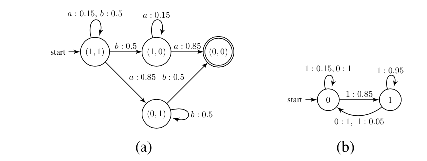
Figure 1: (a) The MDP for the robotic arm controlled by the autonomous controller. A state $(n,m)$ represents there are $n$ small objects and $m$ large objects remaining to be picked. The available actions are $a$ and $b$ for picking up small and large objects, respectively. The MDP for the robotic arm tele-operated by the human can be obtained by changing the probabilities on the transitions. (b) The MDP $M_{C}$ for modeling the dynamics of human’s attention changes.

Given two MDPs, $M_{A}$ for the controller and $M_{H}$ for the operator, and a cognitive model for the operator $M_{C}$, we construct a shared autonomy stochastic systems as an MDP as follows.

$$M_{SA}=\langle\bm{S},\Sigma,\bm{T},D_{0},\mathcal{AP},L,\mathsf{Cost},\gamma\rangle$$

where $\bm{S}=S\times H$ is the set of states. A state $(s,h)$ includes a state $s$ of the system and a cognitive state $h$ of human. $\Sigma=(\Sigma_{A}\cup\Sigma_{H})\times E$ is the set of actions. If $(a,e)\in\Sigma_{A}\times E$, the system is controlled by the autonomous controller and the event affecting human’s cognition is $e$. If $(a,e)\in\Sigma_{H}\times E$, the system is controlled by human operator and the event affecting human’s cognition is $e$. $\bm{T}:\bm{S}\times\Sigma\times\bm{S}\rightarrow[0,1]$ is the transition probability function, defined as follows. Given a state $(s,h)$ and action $(a,e)\in\Sigma_{A}\times E$, $\bm{T}((s,h),(a,e),(s^{\prime},h^{\prime}))=T_{A}(s,a,s^{\prime})T_{C}(h,e,h^{\prime})$, which expresses that the controller acts and triggers an event that affects the operator’s cognitive state. Given a state $(s,h)$ for $h\in H_{s}$, and action $(a,e)\in\Sigma_{H}\times E$, $\bm{T}((s,h),(a,e),(s^{\prime},h^{\prime}))=T_{H}(q,a,q^{\prime})T_{C}(h,e,h^{\prime})$, which expresses that the operator controls the system and an event $e$ happens and may affect the cognitive state. $D_{0}:S\times H\rightarrow[0,1]$ is the initial distribution. $D_{0}(s,h)=D^{M}_{0}(s)\times D^{H}_{0}(h)$, for all $s\in S$, $h\in H$. $L:\bm{S}\rightarrow 2^{\mathcal{AP}}$ is the labeling function such that $L((s,h))=L(s)$. $\mathsf{Cost}:\bm{S}\times\Sigma\times\bm{S}\rightarrow R$ is a cost function for human effort defined over the state and action spaces and $\mathsf{Cost}((s,h),(a,e),(s^{\prime},h^{\prime}))=\mathsf{Cost}(h,e,h^{\prime})$. $\gamma\in(0,1)$ is the discount factor, the same in $M_{C}$. Slightly abusing the notation, we denote the cost function in $M_{SA}$ the same as the cost function in $M_{C}$ and the labeling function in $M_{SA}$ the same as the labeling function in $M$.

Note that, although the cost of human effort only contains the cost in his cognitive model, it is straightforward to incorporate the cost of human’s actions into the cost function.

Example 1

(Cont.) We construct MDP $M_{SA}$ in Figure 2 for the robotic arm example. For example, $\bm{T}((1,1),0),(a_{A},1),((0,1),1))=T((1,1),a_{A},(0,1))\cdot T_{C}(0,1,1)=0.75\cdot 0.85=0.7225$, which means the probability of the robot successfully picking up a small object and placing it into the box while the human changes his cognitive state to 1 (fully focused) upon the robot’s request is $0.7225$. Also it is noted that from the states $((0,1),0)$ and $((1,1),0)$, no human’s action is enabled. The cost function is defined such that $\mathsf{Cost}((q,h),a,(q,h^{\prime}))=10$ if $h^{\prime}=1$, otherwise $5$.

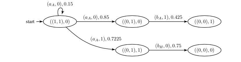
Figure 2: A fragment of MDP $M_{SA}$ for robotic arm example (note only a subset of states and transitions are shown). Subscripts $A$ and $H$ distinguish actions performed by the autonomous controller ($A$) and the human ($H$), respectively.

The main problem we solve is the following.

Problem 1

Given a stochastic system under shared autonomy control between an operator and an autonomous controller, modeled as MDPs $M_{H}$ and $M_{A}$, a model of human’s cognition $M_{C}$, and an LTL specification $\varphi$, compute a policy that is Pareto optimal with respect to two objectives: 1) Maximizing the discounted probability of satisfying the LTL specification $\varphi$ and 2) minimizing the discounted total cost of human effort over an infinite horizon.

The definition of Pareto optimality in this context is given formally at the beginning of section IV-A. By following a Pareto optimal policy, we achieve a balance between two objectives: It is impossible to make one better off without making the other one worse off.

IV Synthesis for shared autonomy policy

Given an MDP $M_{SA}=\langle\bm{S},\Sigma,\bm{T},D_{0},\mathcal{AP},L,\mathsf{Cost},\gamma\rangle$ and a DRA $\mathcal{A}_{\varphi}=\langle Q,2^{\mathcal{AP}},\delta,I,\{(J_{i},K_{i})\mid i=1,\ldots,m\}\rangle$, the product MDP following Definition 2 is $\mathcal{M}=M_{SA}\ltimes\mathcal{A}_{\varphi}=\langle V,\Sigma,\Delta,\bm{D}_{0},\mathsf{Cost}^{\mathcal{M}},\gamma,\mathsf{Acc}\rangle$. Recall that the policy maximizing the probability of satisfying the LTL specification is obtained by first computing the set of AECs in $\mathcal{M}$ and then finding a policy that maximizing the probability of hitting the set $\mathcal{W}$ of states contained in AECs (see Section II-B).

For quantitative LTL objectives, for example, maximizing the probability of satisfying an LTL formula, or a discounted reward objective over an infinite horizon, a memoryless policy in the product MDP suffices for optimality [19, 20]. In the following, by policies, we mean memoryless ones in the product MDP.

Problem 1 is in fact a multi-objective optimization problem for which we need to balance the cost of human’s effort and satisfaction for LTL constraints. However, the solutions for multi-objective MDPs cannot be directly applied due to the constraint that once the system runs into an AEC of $\mathcal{M}$, the policy should be constrained such that all states in that AEC are visited infinitely often. Based on the particular constraint, we divide the original problem into a two-stage optimization problem: The policy synthesis for AECs is separated from solving a multi-objective MDP formulated before reaching a state in an AEC.

IV-A Pareto efficiency before reaching the AECs

The first stage is to balance between a quantitative criterion for a temporal logic objective and a criterion with respect to the cost of human effort before a state in the set $\mathcal{W}$ is reached. Remind that $\mathcal{W}$ is the union of states in the accepting end components of $\mathcal{M}$. We formulate it as an multi-objective MDP. However, for objectives of different types, such as, discounted, undiscounted, and limit-average. the scalarization method for solving multi-objective MDPs does not apply. Thus, we consider to use the discounted reachability property [21] for the given LTL specification, as well as discounted costs for the human attention, with the same discount factor $\gamma\in(0,1)$ specifying the relative importance of immediate rewards.

For an LTL specification, discounting in the state sequence before reaching the set $\mathcal{W}$ means that the number of steps for reaching $\mathcal{W}$ is concerned [21]. Without discounting, as long as two policies have the same probability of reaching the set $\mathcal{W}$, they are equivalent regardless of their expected numbers of steps to reach $\mathcal{W}$. With discounting though, a policy has smaller expected number of steps in reaching $\mathcal{W}$ is considered to be better than the other.

Definition 5

Given the product MDP $\mathcal{M}$, for a state $v$ in $\mathcal{M}$, the discounted probability for reaching the set $\mathcal{W}$ under policy $f:V\setminus\mathcal{W}\rightarrow\mathcal{D}(\Sigma)$ is

$$U_{1}(v,f)=\mathbb{E}^{f}_{v}\left[\sum_{t=0}^{\infty}\gamma^{t}\cdot r_{1}(X_{t},A_{t},X_{t+1})\right]$$

where the reward function $r_{1}:V\times\Sigma\times V\rightarrow\{0,1\}$ is defined such that $r_{1}(v,a,v^{\prime})=1$ if and only if $v\notin\mathcal{W}$ and $v^{\prime}\in\mathcal{W}$, otherwise $r_{1}(v,a,v^{\prime})=0$. The discounted total reward with respect to human attention for a policy $f:V\setminus\mathcal{W}\rightarrow\mathcal{D}(\Sigma)$ and a state $v$ is

$$U_{2}(v,f)=\mathbb{E}^{f}_{v}\left[\sum_{t=0}^{\infty}\gamma^{t}\cdot r_{2}(X_{t},A_{t},X_{t+1})\right],$$

where the reward function $r_{2}:V\times\Sigma\times V\rightarrow\mathbb{R}$ is defined such that $r_{2}(v,a,v^{\prime})=-\mathsf{Cost}^{\mathcal{M}}(v,a,v^{\prime})$ if and only if $v\notin\mathcal{W}$ and $v^{\prime}\notin\mathcal{W}$, $r_{2}(v,a,v^{\prime})=-U_{\mathsf{AEC}}^{\ast}(v^{\prime})$ if $v\notin\mathcal{W}$ and $v^{\prime}\in\mathcal{W}$, and $r_{2}(v,a,v^{\prime})=0$ otherwise. Here, $U_{\mathsf{AEC}}^{\ast}:\mathcal{W}\rightarrow\mathbb{R}$ is the discounted cost of human attention for remaining in an accepting end components under the optimal policy for the second stage. $\blacksquare$

The discounted value profile, at $v$ for policy $f$, is defined as $\vec{U}(v,f)=(U_{1}(v,f),U_{2}(v,f))$. We denote $\vec{r}=(r_{1},r_{2})$ as the vector of reward functions. The function $U_{\mathsf{AEC}}^{\ast}:\mathcal{W}\rightarrow\mathbb{R}$ is computed in the next section.

Definition 6

[8] Given an MDP $\mathcal{M}=\langle V,\Sigma,\Delta\rangle$ and a vector of reward functions $\vec{r}=(r_{1},r_{2},\ldots,r_{n})$, for a given state $v\in V$, policy $f$ Pareto-dominates policy $f^{\prime}$ at state $v$ if and only if $\vec{U}(v,f)=(U_{1}(v,f),\ldots,U_{n}(v,f))\neq\vec{U}(v,f^{\prime})=(U_{1}(v,f^{\prime}),\ldots,U_{n}(v,f^{\prime}))$ and for all $i=1,\ldots,n,U_{i}(v,f)\geq U_{i}(v,f^{\prime})$. A policy $f$ is Pareto optimal in a state $v\in V$ if there is no other policy $f^{\prime}$ Pareto-dominating $f$. For a Pareto-optimal policy $f$ at state $v$, the corresponding value profile $\vec{U}(v,f)$ is referred to as a Pareto-optimal point (or an efficient point). The set of Pareto-optimal point are called the Pareto set. $\blacksquare$

A Pareto optimal policy $f$ for a given initial distribution is defined analogously by comparing the expectations of value functions under the initial distribution.

We employ Tchebycheff scalarization method [22, 11] to find Pareto optimal policies for user specified weights. First, we solve a set of single objective MDPs, one for each reward function. Let $U_{i}(\cdot,f_{i}^{\ast}):V\rightarrow\mathbb{R}$ be the value function of the optimal policy $f_{i}^{\ast}$ with respect to the $i$-th reward function. The ideal point $U^{I}=(U_{1}^{I},U_{2}^{I})$ is then computed as follows: for $i=1,2$, $U_{i}^{I}=\sum_{v\in V}\bm{D}_{0}(v)U_{i}(v,f_{i}^{\ast})$. Given a weight vector $\vec{w}=(w_{1},w_{2})$ where $w_{i}$ is the weight for the $i$-th criterion such that $w_{1}+w_{2}=1$, a Pareto optimal policy associated with the weight vector $\vec{w}$ can be found with the following nonlinear program:

$$\small\begin{split}&\min_{x}\max_{i=1,2}(\lambda_{i}\cdot(U^{I}_{i}-R_{i}\cdot x))+\epsilon\sum_{i=1,2}\lambda_{i}\cdot\left(U^{I}_{i}-R_{i}\cdot x\right)\\ &\text{subject to: }\forall v\in V\setminus\mathcal{W},\\ &\sum_{a\in\Gamma(v)}x(v,a)=\bm{D}_{0}(v)+\gamma\sum_{v^{\prime}\in V}\sum_{a^{\prime}\in\Gamma(v^{\prime})}\Delta(v^{\prime},a^{\prime},v)\cdot x(v^{\prime},a^{\prime}),\\ &\text{and }\forall v\in V\setminus\mathcal{W},\forall a\in\Sigma,\quad x(v,a)\geq 0,\quad\end{split}$$ (1)

where $\epsilon$ is a small positive real that can be chosen arbitrarily, $x(v,a)$ is interpreted as the expected discounted frequency of reaching the state $v$ and then choosing action $a$, $R_{i}\cdot x=\sum_{v\in V}\sum_{a\in\Gamma(v)}\sum_{v^{\prime}\in V}r_{i}(v,a,v^{\prime})\Delta(v,a,v^{\prime})x(v,a)$, and $\vec{\lambda}$ is a positive weighting vector computed from a weight $\vec{w}$, the ideal points and the Nadir points [22] for all reward functions (detailed in Appendix). The nonlinear programming problem can then be formulated into a linear programming problem in the standard way by setting a new variable $z=\max_{i=1,2}(\lambda_{i}\cdot(U^{I}_{i}-R_{i}\cdot x))$. The Pareto optimal policy $f:V\rightarrow\mathcal{D}(\Sigma)$ is defined such that

$$f(v)(a)=\frac{x(v,a)}{\sum_{a\in\Gamma(v)}x(v)},$$ (2)

which selects action $a$ with probability $f(v)(a)$ from the state $v$, for all $v\in V$, $a\in\Gamma(v)$.

Example 2

Continue with the robot arm example. Given the discount factor $\gamma=0.98$, for the simple objective ($1$st objective) as quickly as possible of reaching a state at which all objects are in the box, the optimal strategy $f_{1}^{\ast}$ is shown in the first row of Table I. Intuitively, the robot starts by requesting the operator to increase his level of attention and wants to switch control to human as soon as possible as the latter has higher probability of success for a pick-and-place maneuver. Alternatively, the optimal policy with respect to minimizing the cost of human effort ($2$nd objective), is to let the robot pick up all the objects since by doing so, eventually all the objects will be collected into the box. The strategy $f_{2}^{\ast}$ is shown in the second row of Table I.

Now suppose that a user gives a weight $0.8$ for the first objective and $0.2$ for the second objective, through normalization, the new weight vector $\vec{\lambda}=(11.93,0.02)$, is obtained with the method in Appendix. By solving the linear programming problem in (1), we obtain a Pareto-optimal policy $f_{P}^{\ast}$ shown in the third row of Table I. Noting that the difference of $f_{P}^{\ast}$ and $f_{1}^{\ast}$ is that when it comes to the small object, if the current human attention is high, the robot will request the human to decrease his attention level and therefore, if the object fails to be picked up through tele-operation, the autonomous controller will take over for picking up the small object. Whileas in $f_{1}^{\ast}$, the robot prefers the human operator to pick up all objects, no matter it is a big one or a small one.

Figure 3 shows the state value for the initial state $v_{0}=((1,1),0)$ with respect to reward functions $r_{1},r_{2}$, under the policies $f_{1}^{\ast}$, $f_{2}^{\ast}$ and a subset of Pareto optimal policies, one for each weight vector $\vec{w}$ in the set $\{(\beta,1-\beta)\mid\beta=\frac{k}{10},k=1,2,\ldots,9\}$.

TABLE I: Policies for pick-and-place task

States:	$((1,1),0)$	$((1,1),1)$	$((1,0),0)$	$((1,0),1)$	$((0,1),1)$	$((0,1),0)$
$f_{1}^{\ast}$:	$(a_{A},1)$	$(b_{H},1)$	$(a_{A},1)$	$(a_{H},1)$	$(b_{H},1)$	$(b_{A},1)$
$f_{2}^{\ast}$ :	$(a_{A},0)$	NA	$(a_{A},0)$	NA	NA	$(b_{A},0)$
$f_{P}^{\ast}$	$(a_{A},1)$	$(b_{H},1)$	$(a_{A},0)$	$(a_{H},0)$	$(b_{H},1)$	$(b_{A},1)$

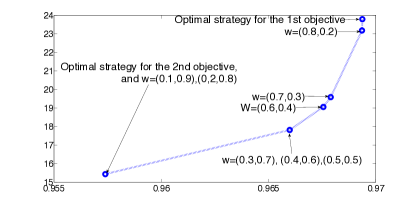
Figure 3: The state values of the initial state with respect to reward functions $r_{1},r_{2}$, under policies $f_{1}^{\ast}$, $f_{2}^{\ast}$ and a set of Pareto optimal policies $f_{P}^{\ast}$, one for each weight vectors in the set $\{(\beta,1-\beta)\mid\beta=\frac{k}{10},k=1,2,\ldots,9\}$. The $x$-axis and $y$-axis represent the values of the initial state under the 1st and 2nd criteria, respectively.

Though the Pareto optimal policy for $\vec{w}=(0.8,0.2)$ is deterministic in this example. It may generally need to be randomized for a given weight vector.

So far we have introduced a method for synthesizing Pareto optimal policies before reaching a state in one of the accepting end components. Next, we introduce a constrained optimization for synthesizing a policy that minimize the expected discounted cost of staying in an AEC and visiting all the states in that AEC infinitely often.

IV-B A constrained optimization for accepting end components

For a state $v$ in $\mathcal{W}$, one can identify at least one AEC $(W,f)$ such that $v\in W$. It is noted that the policy $f:V\rightarrow\mathcal{D}(\Sigma)$ is a randomized policy that ensures every state in $W$ is visited infinitely often with probability 1 [15]. However, there might be more than one AEC that contains a state $v$, and we need to decide which AEC to stay in such that the expected discounted cost of human effort for the control execution over an infinite horizon is minimized.

We consider a constrained optimization problem: For each AEC $(W,f)$ where $W\subseteq V$ and $f:W\rightarrow\mathcal{D}(\Sigma)$, solve for a policy $g:W\rightarrow\mathcal{D}(\Sigma)$ such that the cost of human effort for staying in that AEC is minimized. The constrained optimization problem is formulated as follows.

$$\small\begin{split}&\min_{g}U_{\mathsf{AEC}}(v,g,W)=\sum_{k=0}^{\infty}\gamma^{k}\cdot\mathbb{E}_{v}^{g}[\mathsf{Cost}^{\mathcal{M}}(X_{t},A_{t},X_{t+1})]\\ &\text{subject to: }\forall v\in W,\mathrm{Pr}^{g}(\forall t,\exists t^{\prime}>t,X_{t^{\prime}}=v)=1,\text{ and }\\ &\forall v\in W,\forall a\notin\Gamma(v),g(v)(a)=0,\end{split}$$ (3)

where the term $\mathrm{Pr}^{g}(\forall t,\exists t^{\prime}>t,X_{t^{\prime}}=v)$ measures the probability of infinitely revisiting state $v$ under policy $g$.

The linear program formulated for solving (3) can be obtained as follows:

$$\small\begin{split}&\min\sum_{v\in V}\sum_{a\in\Gamma(v)}\left[x(v,a)\cdot\left(\sum_{v^{\prime}\in V}\mathsf{Cost}^{\mathcal{M}}(v,a,v^{\prime})\Delta(v,a,v^{\prime})\right)\right]\\ &\text{subject to: for }v\in W,\\ &\sum_{a\in\Gamma(v)}x(v,a)=\eta(v)+\gamma\sum_{v^{\prime}\in V}\sum_{a^{\prime}\in\Gamma(v^{\prime})}\Delta(v^{\prime},a^{\prime},v)\cdot x(v^{\prime},a^{\prime}),\\ &\forall v\in W,\forall a\in\Sigma,x(v,a)\geq 0,\\ &\forall v\in W,\sum_{a\in\Gamma(v)}x(v,a)>=\varepsilon,\text{ and }\\ &\forall v\in W,\forall a\notin\Gamma(v),x(v,a)=0,\end{split}$$ (4)

where $\varepsilon$ is an arbitrarily small positive real. $\eta:W\rightarrow[0,1]$ is the initial distribution of states when entering the set $W$. Because for single objective optimization the optimal state value does not depend on the initial distribution [23], $\eta$ can be chosen arbitrarily from the set of distributions over $W$. The physical meaning of $\sum_{a\in\Gamma(v)}x(v,a)$ is the discounted frequency of visiting the state $v$, which is strictly smaller than the frequency of visiting the state $v$ as long as $\gamma\neq 1$. By enforcing the constraints $\sum_{a\in\Gamma(v)}x(v,a)>=\varepsilon$, we ensure that the frequency of visiting every state in $W$ is non-zero, i.e., all states in $W$ will be visited infinitely often.

The solution to (4) produces a memoryless policy $g^{\ast}:W\rightarrow\mathcal{D}(\Sigma)$ that chooses action $a$ at a state $v$ with probability $g^{\ast}(v)(a)=\frac{x(v,a)}{\sum_{a\in\Gamma(v)}x(v,a)}$. Using policy evaluation [24], the state value $U_{\mathsf{AEC}}^{\ast}(v,W)$ for each $v\in W$ under the optimal policy $g^{\ast}$ can be computed. Then, the terminal cost $U_{\mathsf{AEC}}^{\ast}:\mathcal{W}\rightarrow\mathbb{R}$ is defined as follows.

$$U_{\mathsf{AEC}}^{\ast}(v)=\min_{(W,f)\in\mathsf{AEC}}U_{\mathsf{AEC}}^{\ast}(v,W)$$

and the policy after hitting the state $v$ is $g$ such that $U_{\mathsf{AEC}}^{g}(v,W)=U_{\mathsf{AEC}}^{\ast}(v,W)=U_{\mathsf{AEC}}^{\ast}(v)$.

We now present Algorithm 1 to conclude the two-state optimization procedure.

Input: The MDP $M_{A},M_{H}$ and $M_{C}$, a specification automaton DRA $\mathcal{A}_{\varphi}$, and a weight $\vec{w}$.

Output: A pareto policy $f$ for the discounted reachability and a partial function $\mathsf{Policy}:V\rightarrow\mathcal{F}$, where $\mathcal{F}$ is the set of randomized policies. $\mathsf{Policy}(v)$ is the policy to follow after state $v$ is reached.

begin

       $\mathcal{M}=$ GetProductMDP $(M_{A},M_{H},M_{C},\mathcal{A}_{\varphi})$;

       $\mathsf{AEC}(\mathcal{M})=$ GetAEC $(\mathcal{M})$ ;

        /* Compute the accepting end components. */

       for $(W,f)\in\mathsf{AEC}$ do

            $g^{\ast}_{W}=$ConstrainedOptAEC $(W,\mathsf{Cost}^{\mathcal{M}})$;

             /* Solve (4). */

             $U_{\mathsf{AEC}}^{\ast}(v,W)=$PolicyEvaluate $(W,\mathsf{Cost}^{\mathcal{M}},g^{\ast}_{W})$;

            

      $\mathcal{W}=\cup_{(W,f)\in\mathsf{AEC}}W$;

       for $v\in\mathcal{W}$ do

            $U_{\mathsf{AEC}}^{\ast}(v)=\min_{(W,f)\in\mathsf{AEC}}U_{\mathsf{AEC}}^{\ast}(v,W)$;

             $\mathsf{Policy}(v)=g^{\ast}_{W}$ for which $W$ such that $U_{\mathsf{AEC}}^{\ast}(v,W)=U_{\mathsf{AEC}}^{\ast}(v)$.

      $\vec{r}=$ GetRewardVec $(\mathcal{M},\{U_{\mathsf{AEC}}^{\ast}(v)\mid v\in\mathcal{W}\},\mathcal{W})$;

       /* Formulate the reward vector according to Definition 5. */

       $f=$GetParetoOptimal $(\vec{r},\mathcal{M},\vec{w})$ /* Solve (1) and obtain the Pareto optimal policy $f$ as in (2). */

       return $f,\mathsf{Policy}$.

Algorithm 1 TwoStageOptimization

Remark

Although in this paper we only considered two objectives, the methods can be easily extended to more than two objectives for handling LTL specifications and different reward/cost structures in synthesis for stochastic systems, for example, the objective of balancing between the probability of satisfying an LTL formula, the discounted total cost of human effort, and the discounted total cost of energy consumption.

V An example on shared autonomy

We apply Algorithm 1 to a robotic motion planning problem in a stochastic environment. The implementations are in Python and Matlab on a desktop with Intel(R) Core(TM) processor and 16 GB of memory.

Figure 4a shows a gridworld environment of four different terrains: Pavement, grass, gravel and sand. In each terrain, the mobile robot can move in four directions (heading north ‘N’, south ‘S’, east ‘E’, and west ‘W’). There is onboard feedback controller that implements these four maneuver, which are motion primitives. Using the onboard controller, the probability of arriving at the correct cell is $95\%$ for pavement, $80\%$ for grass, $75\%$ for gravel and $65\%$ for sand. Alternatively, if the robot is operated a human, it can implement the four actions with a better performance for terrains grass, sand and gravel. The probability of arriving at the correct cell under human’s operation is $95\%$ for pavement, $90\%$ for grass, $85\%$ for gravel and $80\%$ for sand. The objective is that either the robot has to visit region $R_{1}$ and then $R_{2}$, in this order, or it needs to visit region $R_{3}$ infinitely often, while avoiding all the obstacles. Formally, the specification is expressed with an LTL formula $\varphi=\left(\lozenge(R_{1}\land\lozenge R_{2})\lor\square\lozenge R_{3}\right)\land\square\lozenge\neg\text{Unsafe}$.

Figure 4b is the cognitive model of the operator, including three states : $L$, $M$ and $H$ represent that human pays low, moderate, and high attention to the system respectively. The costs of paying low, moderate and high attention to the system are $1$, $5$, and $10$, respectively. Action ‘$+$’ (resp. ’$-$’) means a request to increase (resp. decrease) the attention and action $\lambda$ means a request to maintain the current attention. The operator takes over control at state $H$.

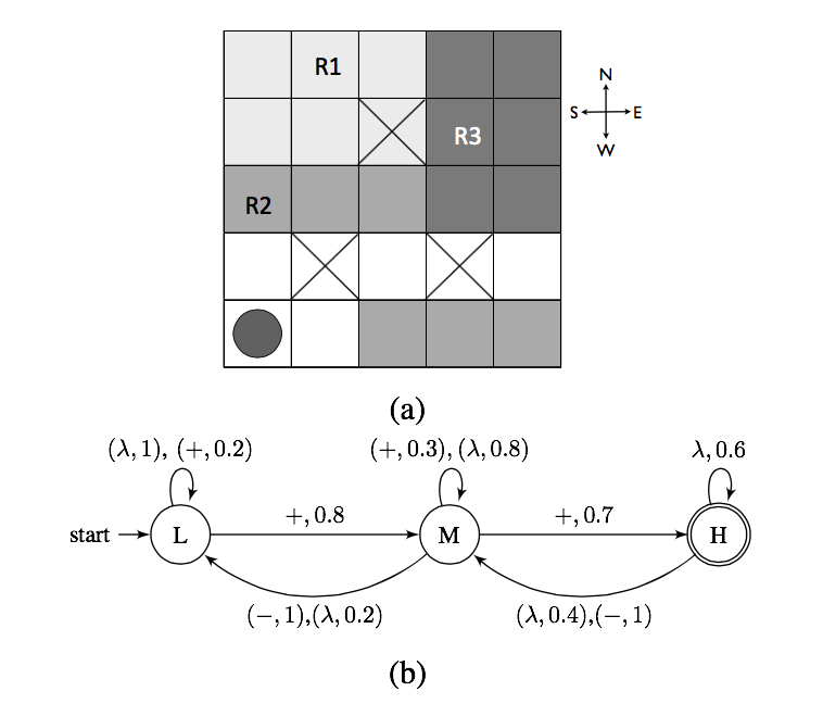
Figure 4: (a) A $5\times 5$ gridworld, where the disk represents the robot, the cells $R_{1}$, $R_{2}$, and $R_{3}$ are the interested regions, the crossed cells are obstacles. We assume that if the robot hits the wall (edges), it will be bounced back to the previous cell. Different grey scales represents different terrains: From the darkest to the lightest, these are “sand,” “grass,” “pavement” and “gravel.” (b) The MDP $M_{C}$ of the human operator.

During control execution, we aim to design a policy that coordinates the switching of control between the operator and the autonomous controller, i.e., onboard software controller. The policy should be Pareto optimal in order to balance between maximizing the expected discounted probability of satisfying the LTL formula $\varphi$, and minimizing the expected discounted total cost of human efforts. Figure 5 shows the state value for the initial state with respect to reward functions $r_{1}$ for the LTL formula and $r_{2}$ for the cost of human effort, under the single objective optimal policy $f_{1}^{\ast}$ and $f_{2}^{\ast}$, and a subset of Pareto optimal policies, one for each weight vectors $\vec{w}$ in the set $\{(\beta,1-\beta)\mid\beta=\frac{k}{10},k=1,2,\ldots,9\}$. For the LTL specification, all policies are randomized.

Figure 5: The state values of the initial state given reward functions $r_{1},r_{2}$, under policies $f_{1}^{\ast}$, $f_{2}^{\ast}$ and a set of Pareto optimal policies $f_{P}^{\ast}$, for each $\vec{w}\in\{(\beta,1-\beta)\mid\beta=\frac{k}{10},k=1,2,\ldots,9\}$. The $x$-axis represents the values of the initial state for discounted probability of satisfying the LTL specification. The $y$-axis represents the values of the initial state with respect to the cost of human effort.

VI Concluding remarks and critiques

We developed a synthesis method for a class of shared autonomy systems featured by switching control between a human operator and an autonomous controller. In the presence of inherent uncertainties in the systems’ dynamics and the evolution of humans’ cognitive states, we proposed a two-stage optimization method to trade-off the human effort for the system’s performance in satisfying a given temporal logic specification. Moreover, the solution method can also be extended for solving multi-objective MDPs with temporal logic constraints. In the following, we discuss some of the limitations in both modeling and solution approach in this paper and possible directions for future work.

We employed two MDPs for modeling the system operated by the human and for representing the evolution of cognitive states triggered by external events such as workload, fatigue and requests for attention. We assumed that these models are given. However, in practice, we might need to learn such models through experiments and then design adaptive shared autonomy policies based on the knowledge accumulated over the learning phase. In this respect, a possible solution is to incorporate joint learning and control policy synthesis, for instance, PAC-MDP methods [25], into multi-objective MDPs with temporal logic constraints.

Another limitation in modeling is that the current cognitive model cannot capture all possible influences of human’s cognition on his performance. Consider, for instance, when the operator is bored or tired, his performance in some tasks can be degraded, and therefore the transition probabilities in $M_{H}$ are dependent on the operator’s cognitive states. In this case, we will need to develop a different product operation for combining the three factors: $M_{A}$, a set of $M_{H}$’s for different cognitive states, and $M_{C}$, into the shared autonomy system. Despite the change in modeling the shared autonomy system, the method for solving Pareto optimal policies developed in this paper can be easily extended.

Appendix A Weight normalization for multi-objective criteria

Consider a multiobjective MDP $\mathcal{M}=\langle V,\Sigma,\Delta,\bm{D}_{0},\vec{r},\gamma\rangle$ where $\vec{r}=(r_{1},r_{2},\ldots,r_{n})$ is a vector of reward functions and $\gamma$ is the discount factor, let $U_{i}(\cdot,f_{i}^{\ast})$ be the vectorial value function optimal for the $i$-th criterion, specified with the reward function $r_{i}$. An approximation of the Nadir point for the $i$-th criterion is computed as follows, $U_{i}^{N}=\sum_{v\in V}\bm{D}_{0}(v)\min_{j=1,\ldots,n}U_{i}(v,f_{j}^{\ast})$ where $U_{i}(\cdot,f_{j}^{\ast})$ is a vector value function obtained by evaluating the optimal policy for the $j$-th criterion with respect to the $i$-th reward function. The weight vector after normalization is defined as $\lambda_{i}=\frac{w_{i}}{\left|U_{i}^{I}-U_{i}^{N}\right|}\enspace.$

References

- [1] B. Pitzer, M. Styer, C. Bersch, C. DuHadway, and J. Becker, “Towards perceptual shared autonomy for robotic mobile manipulation,” in IEEE International Conference on Robotics and Automation, May 2011, pp. 6245–6251.
- [2] K. Kinugawa and H. Noborio, “A shared autonomy of multiple mobile robots in teleoperation,” in Proceedings of IEEE International Workshop on Robot and Human Interactive Communication, 2001, pp. 319–325.
- [3] S. Gnatzig, F. Schuller, and M. Lienkamp, “Human-machine interaction as key technology for driverless driving - a trajectory-based shared autonomy control approach,” in IEEE International Symposium on Robot and Human Interactive Communication, Sept 2012, pp. 913–918.
- [4] W. Li, D. Sadigh, S. Sastry, and S. Seshia, “Synthesis for human-in-the-loop control systems,” in Tools and Algorithms for the Construction and Analysis of Systems, ser. Lecture Notes in Computer Science, E. Ábrahám and K. Havelund, Eds. Springer Berlin Heidelberg, 2014, vol. 8413, pp. 470–484.
- [5] A. Pentland and A. Liu, “Modeling and prediction of human behavior,” Neural Computation, vol. 11, no. 1, pp. 229–242, 1999.
- [6] C. A. Rothkopf and D. H. Ballard, “Modular inverse reinforcement learning for visuomotor behavior,” Biological cybernetics, vol. 107, no. 4, pp. 477–490, 2013.
- [7] C. L. McGhan, A. Nasir, and E. Atkins, “Human intent prediction using markov decision processes,” in Proceedings of Infotech Aerospace Conference, 2012.
- [8] K. Chatterjee, R. Majumdar, and T. A. Henzinger, “Markov decision processes with multiple objectives,” in Symposium on Theoretical Aspects of Computer Science. Springer, 2006, pp. 325–336.
- [9] K. Chatterjee, “Markov decision processes with multiple long-run average objectives,” in FSTTCS 2007: Foundations of Software Technology and Theoretical Computer Science, ser. Lecture Notes in Computer Science, V. Arvind and S. Prasad, Eds. Springer Berlin Heidelberg, 2007, vol. 4855, pp. 473–484.
- [10] V. Forejt, M. Kwiatkowska, and D. Parker, “Pareto curves for probabilistic model checking,” in Proceedings of 10th International Symposium on Automated Technology for Verification and Analysis, ser. LNCS, S. Chakraborty and M. Mukund, Eds., vol. 7561. Springer, 2012, pp. 317–332.
- [11] P. Perny and P. Weng, “On finding compromise solutions in multiobjective markov decision processes,” in Proceedings of the 19th European Conference on Artificial Intelligence. IOS Press, 2010, pp. 969–970.
- [12] I. Das and J. E. Dennis, “A closer look at drawbacks of minimizing weighted sums of objectives for pareto set generation in multicriteria optimization problems,” Structural optimization, vol. 14, no. 1, pp. 63–69, 1997.
- [13] E. A. Emerson, “Temporal and modal logic,” Handbook of Theoretical Computer Science, Volume B: Formal Models and Sematics (B), vol. 995, p. 1072, 1990.
- [14] L. De Alfaro, “Formal verification of probabilistic systems,” Ph.D. dissertation, Stanford University, 1997.
- [15] K. Chatterjee, M. Henzinger, M. Joglekar, and N. Shah, “Symbolic algorithms for qualitative analysis of markov decision processes with büchi objectives,” Formal Methods in System Design, vol. 42, no. 3, pp. 301–327, 2013.
- [16] D. Henriques, J. G. Martins, P. Zuliani, A. Platzer, and E. M. Clarke, “Statistical model checking for markov decision processes,” in 9th International Conference on Quantitative Evaluation of Systems, 2012, pp. 84–93.
- [17] M. A. Goodrich and A. C. Schultz, “Human-robot interaction: a survey,” Foundations and trends in human-computer interaction, vol. 1, no. 3, pp. 203–275, 2007.
- [18] A.-I. Mouaddib, S. Zilberstein, A. Beynier, L. Jeanpierre, et al., “A decision-theoretic approach to cooperative control and adjustable autonomy.” in European Conference on Artificial Intelligence, 2010, pp. 971–972.
- [19] C. Baier, J.-P. Katoen, et al., Principles of model checking. MIT press Cambridge, 2008, vol. 26202649.
- [20] J. Filar and K. Vrieze, Competitive Markov Decision Processes. New York, NY, USA: Springer-Verlag New York, Inc., 1996.
- [21] L. de Alfaro, M. Faella, T. A. Henzinger, R. Majumdar, and M. Stoelinga, “Model checking discounted temporal properties,” Theoretical Computer Science, vol. 345, no. 1, pp. 139–170, 2005.
- [22] R. E. Steuer, Multiple Criteria Optimization: Theory, Computation and Application. Radio e Svyaz, Moscow, 504 pp., 1992, (in Russian).
- [23] M. L. Puterman, Markov decision processes: discrete stochastic dynamic programming. John Wiley & Sons, 2009, vol. 414.
- [24] A. G. Barto, Reinforcement learning: An introduction. MIT press, 1998.
- [25] J. Fu and U. Topcu, “Probably approximately correct mdp learning and control with temporal logic constraints,” in Proceedings of Robotics: Science and Systems, Berkeley, USA, July 2014.