Transcriptional leakage versus noise: A simple mechanism of conversion between binary and graded response in autoregulated genes

Abstract

We study the response of an autoregulated gene to a range of concentrations of signal molecules. We show that transcriptional leakage and noise due to translational bursting have the opposite effects. In a positively autoregulated gene, increasing the noise converts the response from graded to binary, while increasing the leakage converts the response from binary to graded. Our findings support the hypothesis that, being a common phenomenon, leaky expression may be a relatively easy way for evolutionary tuning of the type of gene response without changing the type of regulation from positive to negative.

I Introduction

Leaky transcription (also called basal transcription) occurs when there is no tight control over the promoter and some level of transcription is maintained even when the promoter is in the off state. To date, the role of transcriptional leakage has been underappreciated. Leaky expression is most often described as unfavorable from the point of view of an experimenter Weber and Fussenegger (2007); Minaba and Kato (2014); Guo and Jia (2014), while little is known about its evolutionary benefit for cells. An obvious fact is that some basal transcription is necessary to initiate the positive feedback Avery (2005). Yanai et al. Yanai et al. (2006) note that, in general, the selection against “unnecessary” transcription is low and hypothesize that leakiness of the promoters may be evolutionarily neutral  Dekel and Alon (2005); Shachrai et al. (2010); Szekely et al. (2013). On the other hand, Ingolia et al. Ingolia and Murray (2007) put forward a hypothesis that, being a common phenomenon, leaky expression may be a relatively easy way for an evolutionary conversion of gene expression from binary to graded and vice versa. They qualitatively demonstrated in the experiments on yeast and in simulations that mutations in the $P_{FUS1}$ promoter sequence entail changes in the basal level of expression of the autoregulated gene, which produces different expression patterns: unimodal or bimodal.

The effectors (signaling molecules) bind or cause phosphorylation of the transcription factors (TFs) thus changing the strength of gene repression or activation  Rosenfeld et al. (2005); Tabaka et al. (2008); Carey et al. (2013). We define the response to the increasing effector concentration as graded when the stationary distribution of responses of individual cells is unimodal for any effector concentration. If bimodal distribution occurs for any range of those concentrations, then the response is binary Kringstein et al. (1998); Becskei et al. (2001). It became a common knowledge that positive autoregulation serves as a mechanism of differentiation of the cell population into phenotypically distinct groups Alon (2007) (which may increase the chances of survival in a changing environment through the bet-hedging strategy  Fraser and Kærn (2009); Beaumont et al. (2009)), while negative autoregulation may be preferred when a precise response is needed Nevozhay et al. (2009); Little et al. (2013).

Let us consider, however, an evolutionary adaptation from the conditions where binary response was favorable to the conditions where graded response is more preferred Ingolia and Murray (2007). The evolutionary change of the nature of gene regulation from positive to negative may be more difficult than fine-tuning of the parameters of positive regulation, such as transcriptional leakage, e.g. due to point mutations in the promoter sequence Ingolia and Murray (2007); Mitrophanov et al. (2010).

Self-regulated genes often occur in two-component signaling systems (TCS) Bijlsma and Groisman (2003); Goulian (2010). These systems respond to external stimuli: Signal molecules bind to the membrane-bound receptors that phosphorylate the TFs, which enables the TFs to bind to the promoter of the target gene. TCS occur mostly in prokaryotes, and are less common in eukaryotes. The majority of TCS are positively autoregulated, but not all of them display bimodal expression Goulian (2010). Known are the TCS with positive feedback and a significant basal transcription, e.g.: $hrpXY$ in E. amylovora Wei et al. (2000), $CpxR$ in E. coli DiGiuseppe and Silhavy (2003), $VirG$ in Agrobacterium tumefaciens Stachel and Zambryski (1986); Yamamoto et al. (1987).

Becskei et al. Becskei et al. (2001) first used the term “conversion from graded to binary response”, but the conversion in their engineered $tetR$ gene circuit was obtained by artificially introducing a feedback loop into an otherwise open-loop system. Mitrophanov et al. Mitrophanov et al. (2010) studied numerically and experimentally the positively autoregulated TCS $PhoP/PhoQ$ in Salmonella enterica with promoter mutations resulting in different basal expression levels. They did not test a wide range of stimulus concentrations but only examined two cases of a low and high stimulus, and the binary response was not found. It is possible that these two stimulus levels represented the extreme cases (near-maximum and near-zero regulation) where the distributions are unimodal, and one should seek for the bimodal response by scanning the intermediate stimulus levels. Mitrophanov et al. Mitrophanov et al. (2010) hypothesized that different evolutionary niches may favor higher or lower levels of basal expression and, consequently, different response levels.

We propose a simple quantitative model (Fig. 1) of an autoregulated gene that allows one to calculate the conditions for conversion between binary and graded response without changing the type of feedback. We show the key role of intrinsic noise and leakage in this “binary-graded” conversion.

II Model of an autoregulated gene

We start from the kinetic scheme shown in Table 1 and make the simplifying assumptions, following Friedman et al.  Friedman et al. (2006): (i) mRNA is short-lived compared to proteins. This means that our simplified model may be suitable for average prokaryotic genes but also for a subset of eukaryotic genes. The Escherichia coli proteome shows insignificant degradation Koch and Levy (1955) with a protein lifetime longer than the duration of a cell cycle but mRNA molecules are short-lived on the time scale of a cell cycle Taniguchi et al. (2010). In yeast, there is a certain percentage of genes that produce unstable mRNAs Geisberg et al. (2014), and the mRNA stability in general depends on environmental conditions Munchel et al. (2011). At the same time, a substantial percentage of yeast proteins are long-lived Belle et al. (2006). For example, the mean ratio $k_{dm}/k_{dp}$ in budding yeast is $>10$ (the median $\approx 3$) for the set of $\sim 2000$ genes Shahrezaei and Swain (2008), showing that the model assumptions are widely met in this eukaryotic organism. (ii) The kinetics of TF binding and unbinding is fast enough to be compressed to the form of the Hill function

$$H(P)=\frac{1}{1+cP^{n}},$$ (1)

Transcription factor binding:
Repressor	Activator
O + nP <=>[c] OP_n	O + nP <=>[1/c] OP_n
mRNA synthesis and degradation:
Repressor	Activator
O ->[k_m] M + O	O ->[k_ml] M + O
OP_n ->[k_ml] M + OP_n	OP_n ->[k_m] M + OP_n
M ->[k_dm] ∅
Transcription factor synthesis and degradation:
M ->[k_p] P + M
P ->[k_dp] ∅

Table 1: Model kinetics. $\mathrm{M}$, mRNA; P, protein; O, operator; n, number of TFs that bind cooperatively to the operator; $c$, signal parameter; $k_{m}$, rate of mRNA synthesis from the operator in the active state; $k_{ml}$, rate of mRNA synthesis from the operator in the inactive state (leakage); $k_{dm}$, rate of mRNA degradation ; $k_{p}$, rate of protein synthesis; $k_{dp}$, rate of protein degradation.

where $P$ is the total number of TFs, $n$ is the cooperativity index, $n>0$ for repression and $n<0$ for activation. (iii) The cooperativity is very strong, such that only the $n$th power of $P$ is present in Eq. (1). The signal of a certain strength activates a certain fraction of TFs (due to phosphorylation, as in TCS, or due to binding of signal molecules). The signal parameter $c$ depends on the fractions of active and inactive TFs as well as on their binding and unbinding rates to the operator (see Appendix A). The assumptions (i–iii) are necessary to make the model analytically tractable.

The operator effectively switches at a high frequency between the two states, O and OP_n, one of which is inactive and the other is active. The operator is active with the probability $H(P)$, and then the mRNA is synthesized at the rate $k_{m}$. Alternatively, the operator is inactive with the probability $1-H(P)$, and then the leaky transcription proceeds at the rate $k_{ml}<k_{m}$. Therefore, at the steady state, $k_{m}H(P)+k_{ml}(1-H(P))=k_{dm}M$. We write the left-hand side divided by $k_{m}$ as

$$h(P)=H(P)(1-\epsilon)+\epsilon,$$ (2)

where $\epsilon=k_{ml}/k_{m}$. The function $h(P)$, which describes the deviation from the maximum possible transcription rate due to regulation and leakage, will be called the transfer function Ochab-Marcinek and Tabaka (2010). The deterministic equation for protein synthesis gives $k_{p}M=k_{dp}P$ at the steady state, where $k_{p}$ is the protein transcription rate and $k_{dp}$ is the protein degradation rate. The deterministic stationary numbers of proteins can be then found by a geometric construction Ochab-Marcinek and Tabaka (2010), as the points of intersections between the transfer function $h(P)$ and a straight line, $H(P)(1-\epsilon)+\epsilon=\frac{1}{\alpha\beta}P$, with $\alpha=k_{m}/k_{dp}$ and $\beta=k_{p}/k_{dm}$. If the straight line intersects the transfer function more than once, then the deterministic model is bistable.

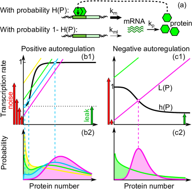
Figure 1: (Color online) The model of an autoregulated gene with leaky transcription [(a), positive regulation]. The intersections of the straight line $L(P)$ and the transfer function $h(P)$ (b1) and (c1) indicate the extrema of the protein distributions (b2) and (c2).

III Extrema of the protein distribution

Based on the work of Friedman et al. Friedman et al. (2006) we calculate the stochastic distribution of $P$ in the autoregulated gene with exponentially distributed translational bursts. We note that in  Friedman et al. (2006) the description of leakage in their transfer function, $\tilde{h}(P)=H(P)+\epsilon$, is only correct when $\epsilon\approx 0$, or if the parameters are reinterpreted ($\tilde{k}_{m}\equiv k_{m}-k_{ml}$, $\tilde{\epsilon}\equiv k_{ml}/(k_{m}-k_{ml})$, $\tilde{\alpha}\equiv(k_{m}-k_{ml})/k_{dp}$; see Appendix C), since otherwise the probabilities of the active and inactive states of the operator would not sum up to 1. Our description is the most natural, as the parameters are simply the reaction rates that follow directly from the kinetics (Table 1). Therefore, the protein distribution in our model differs from that in Friedman et al. (2006):

$$p(P) =AP^{-1}e^{-P/\beta}e^{\alpha\int dP\ h(P)/P}$$ (3)

$$=AP^{\alpha-1}e^{-P/\beta}H(P)^{\alpha(1-\epsilon)/n}.$$

Here $\alpha=k_{m}/k_{dp}$, $\beta=k_{p}/k_{dm}$ is interpreted as the mean burst size, and $A$ is a normalization constant. Note also that $\alpha$ should be interpreted as the maximum mean frequency of translational bursts that can be achieved by the system in the theoretical limit of $c=0$ (see Appendix D). In a certain range of the regulation strength $c$, the distribution $p(P)$ can be bimodal. The conditions for bimodality can be determined by calculation of the extrema of the distribution: $\frac{dp(P)}{dP}=0$  Ochab-Marcinek and Tabaka (2010); Mackey et al. (2010); Aquino et al. (2012). In the present stochastic model, the extrema of $p(P)$ are again given by the points of intersections between the transfer function $h(P)$ and a straight line (which we will denote by $L(P)$):

$$H(P)(1-\epsilon)+\epsilon=\frac{1}{\alpha\beta}P+\frac{1}{\alpha}$$ (4)

The geometric construction is almost the same as in the deterministic case but there appears the noise term $1/\alpha$. It shifts the positions of the extrema with respect to the deterministic stationary states. Therefore, the noise may induce a bifurcation in the parameter range in which the deterministic model does not predict bistability Horsthemke and Lefever (1984). Interestingly, this noise-induced shift depends on the maximum burst frequency $\alpha$ only, and not on the burst size $\beta$. In the limit of infinitely frequent bursting, the stochastic term $1/\alpha$ disappears and the extrema of the protein distribution overlap with the deterministic stationary states. Therefore, we will use $1/\alpha$ as a measure of the minimum noise that can be achieved by the system at the theoretical limit of $c=0$.

IV Binary and graded response to a signal

Using the geometric construction (4), we examine how the protein distributions behave when the regulation strength $c$ is varied. The change in $c$ corresponds to the change in the effector concentration which controls the strength of gene regulation. To obtain precise regulation, the gene response should be graded for the whole possible range of $c$. The following conclusions follow from the geometric construction (see Appendix E for a detailed analysis): Transcriptional leakage narrows the range of regulation. Negative feedback allows for a graded response only, because at most one intersection of $L(P)$ and $h(P)$ is possible due to their different monotonicity. When the feedback is positive, binary response is possible. For $\epsilon<1/\alpha<1$, the response is always binary (also for $n=-1$, consistently with the results of Friedman et al. (2006), the case not predicted by the deterministic model).

Our central result is that transcriptional leakage counteracts the stochastic effect of bursting, by converting binary response into graded response. This is because $\epsilon>0$ shifts the base of the transfer function upwards, in such a way that, if the leakage is sufficiently large, it may enable only one intersection of $h(P)$ and $L(P)$.

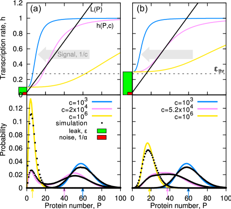
Figure 2: (Color online) Transcriptional leakage converts binary response into graded response and counteracts the effect of noise. Binary response occurs for the leakage below the threshold $\epsilon_{thr}$, when $1/\alpha<1$ (dashed line). Otherwise, graded response occurs. (Dots) Mesoscopic simulations of the gene regulation kinetics using the Gillespie algorithm Gibson and Bruck (2000)). (a) $\epsilon=0.1$. (b) $\epsilon=0.3$. Parameters are as follows: $n=-3$, $\alpha=30$, $\beta=2$, $\epsilon_{thr}=0.275$. (Arrows) Mean values of the distributions.

Below, we calculate the condition for the graded response in the general case of $n<0$, when $1/\alpha<1$. We note that for given $\alpha$ and $\beta$ there exists a value $c=c^{*}$ for which $L(P)$ intersects $h(P,c^{*})$ in its inflection point. The inflection point is the point in which $h(P)$ has the greatest slope, and this slope increases monotonically as $c$ decreases. Therefore, if the slope of $L(P)$ intersecting $h(P,c^{*})$ in its inflection point is greater than the slope of $h(P,c^{*})$, then $L(P)$ will intersect $h(P,c)$ only once for any $c$. We write this condition as:

$$h(P_{p},c^{*})=\frac{1}{\alpha\beta}P_{p}+\frac{1}{\alpha} \ \mathrm{and} \frac{d}{dP_{p}}h(P_{p},c^{*})<\frac{1}{\alpha\beta},$$ (5)

where $P_{p}=\left[(n-1)/\left(c^{*}(n+1)\right)\right]^{1/n}$ is the value of $P$ in the inflection point. Knowing that $H(P_{p})=(n+1)/(2n)$ for any $c$, and $H^{\prime}(P_{p})=-(n^{2}-1)/(4nP_{p})$, we get:

$$\epsilon>\frac{1}{\alpha}\frac{(-4n)}{(n-1)^{2}}+\frac{(n+1)^{2}}{(n-1)^{2}}\equiv\epsilon_{thr}$$ (6)

The above condition says that if the transcriptional leakage $\epsilon$ is greater than the threshold $\epsilon_{thr}$, then the positively autoregulated gene will produce a graded response. For the leakage below that threshold, the response will be binary (Fig. 2). The condition (6) depends only on the cooperativity $n$ and the maximum burst frequency $\alpha$, but not on the burst size $\beta$. Since $n<0$ for activation, both the noise and the cooperativity increase $\epsilon_{thr}$, which makes the graded response more difficult to obtain. This finding is consistent with the experimental observation of Ingolia et al. Ingolia and Murray (2007) that bimodal distributions are found for low basal expression and high induced expression (which corresponds to a steeper transfer function).

V Conclusions

The above calculation based on a geometric construction reveals the constructive role of transcriptional leakage in gene regulation: The leakage in a positively autoregulated gene acts against the translational noise as a factor that controls the conversion between binary and graded response. While increasing the noise induces binary response, increasing the leakage recovers graded response. However, this conversion is obtained at the cost of narrowing the range of regulation. Therefore, the leakage can be disadvantageous in the case of negative autoregulation (because the response is anyway graded), but it can be beneficial in the case of positive autoregulation, when it is needed to prevent the binary response. Leakage strength can be tuned by single mutations in the promoter Ingolia and Murray (2007), whereas keeping the same direction of the response after the positive to negative feedback conversion would also require the reversal of the signal effect on the TF (if a high concentration of signal molecules strengthened the binding of the activator to the promoter, now it should cause a weaker binding of the repressor). The conversion of the feedback type is thus a much less probable evolutionary scenario because it would require multiple mutations (within the TF’s effector binding site and its DNA-binding domain) while simultaneously keeping the TF function. Our findings may therefore provide a quantitative support for the experimentally based hypothesis Ingolia and Murray (2007); Mitrophanov et al. (2010) that, being a common phenomenon, leaky expression can be an easier way of adaptation of the gene response type to different evolutionary niches than the change of the feedback type from positive to negative.

Appendix A Signal parameter $c$

Below, we show how the coefficient $c$ in the Hill function $H(P)$ contains the information about the signal strength. For simplicity, we take the example of $n=1$. $P=P_{a}+P_{i}$ denotes the total number of transcription factors (TFs), both active and inactive. $k_{on}^{a}$, $k_{off}^{a}$ denote the binding and unbinding rates of the active TF to the operator. $k_{on}^{i}$, $k_{off}^{i}$ are the binding and unbinding rates for the inactive TF. Then,

$$H(P)= \frac{1}{1+\frac{k_{on}^{a}}{k_{off}^{a}}P_{a}+\frac{k_{on}^{i}}{k_{off}^{i}}P_{i}}$$ (7)

$$= \frac{1}{1+P\left[\frac{k_{on}^{a}}{k_{off}^{a}}f_{a}+\frac{k_{on}^{i}}{k_{off}^{i}}(1-f_{a})\right]}$$

$$= \frac{1}{1+cP}.$$

$f_{a}$ denotes the active fraction of all TFs, e.g. the fraction of phosphorylated TFs in the case of a two-component system (assuming that phosphorylation and dephosphorylation rates are such that this fraction remains constant on the time scales of other reactions). In the case of binding of a signal molecule (effector) E, $f_{a}=g(E)$ is a Hill function describing the effector binding to the TF (under the assumption that $E\gg P$ and that the effector-TF binding and unbinding rates are much faster than the time scales of other reactions in the system).

For $n>1$, $H(P)$ is constructed in an analogous way under the assumption of very strong cooperativity. Although mixed terms may appear [e.g. for $n=2$, $P_{a}P_{i}(k_{on,1}^{a}k_{on,2}^{i})/(k_{off,1}^{a}k_{off,2}^{i})$ etc., where the number in the subscript denotes binding of the first or the second TF], they can still be written in the form of $P^{n}\cdot const$. And therefore, the coefficient $c$ will still contain the particular binding/unbinding rates and the details of the TF-effector interactions.

Appendix B Limiting cases

Note that $c=c(f_{a})$ varies between finite values as the fraction $f_{a}$ varies from 0 to 1. In the case of $n=1$, as in the example (7), $c(f_{a}=0)=k_{on}^{i}/k_{off}^{i}$ and $c(f_{a}=1)=k_{on}^{a}/k_{off}^{a}$. This means that $H(P)=0$ and $H(P)=1$ are the theoretical limits for an extremely strong or weak signal when the binding of active TFs is infinitely fast and the binding of inactive TFs is infinitely slow compared to unbinding. These two limits correspond to non-regulated genes Friedman et al. (2006); Shahrezaei and Swain (2008), i.e. Gamma distributions with the means $\alpha\beta$ and $\alpha\beta\epsilon$.

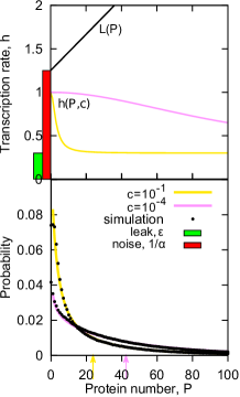
Figure 3: (Color online) When bursts are rare, $\alpha<1$, then the maximum of the protein distribution $p(P)$ is always at $P_{max}=0$ independently of the leakage rate $\epsilon$ and the regulation strength $c$. This is because there is no intersections between the straight line $L(P)$ and the transfer function $h(P)$. Parameter values are as follows: $n=2$, $\alpha=0.8$, $\beta=60$, $\epsilon=0.3$. Arrows mark the mean values of the shown distributions.

Appendix C Reinterpretation of the parameters of the formula used in Friedman et al. (2006)

The formula proposed by Friedman et al. Friedman et al. (2006) to describe the protein distribution produced by an autoregulated gene,

$$p(P)=AP^{\tilde{\alpha}(1+\tilde{\epsilon})-1}e^{-P/\beta}H(P)^{\tilde{\alpha}/n},$$ (8)

can be made formally equivalent to our formula (3), if the parameters of (8) are reinterpreted.

In our model, the total transcription rate is:

$$k_{m}H(P)+k_{ml}(1-H(P))=$$ (9)

$$= H(P)(k_{m}-k_{ml})+k_{ml}$$

$$\equiv k_{m}[H(P)(1-\epsilon)+\epsilon]$$

$$\equiv k_{m}h(P)$$

where $k_{m}$ is the transcription rate in the case when the operator is in the active state. This is the maximum possible transcription rate, which can be achieved if the operator is on all the time. $k_{ml}$ is the transcription rate in the case when the operator is in the inactive state (leaky transcription). $\epsilon=k_{ml}/k_{m}$ measures the ratio of the transcription rate in the inactive state to the transcription rate in the active state. The transfer function $h(P)$ measures the deviation from the maximum possible transcription rate due to regulation and leakage.

Friedman et al. use a different transfer function: $\tilde{h}(P)=H(P)+\tilde{\epsilon}$. The total transcription rate is then

$$\tilde{k}_{m}[H(P)+\tilde{\epsilon}]\equiv\tilde{k}_{m}\tilde{h}(P).$$ (10)

In order to make it equivalent to (9), one must assume $\tilde{k}_{m}=k_{m}-k_{ml}$ and $\tilde{\epsilon}=k_{ml}/\tilde{k}_{m}$. With this interpretation of the parameters, the formulas (8) and (3) for the protein distributions will be equivalent, provided that $\tilde{\alpha}=\tilde{k}_{m}/k_{dp}$, whereas in our model $\alpha=k_{m}/k_{dp}$.

It should be noted that $\tilde{k}_{m}$ is not the transcription rate $k_{m}$ shown in the kinetic scheme (Table I in the main manuscript). Therefore, our notation (without tilde) is more natural because it follows directly from the kinetics.

At this point, we note that neither the interpretation of $\tilde{\alpha}$ nor $\alpha$ as “the mean number of bursts per cell cycle” (as in Friedman et al. (2006)) is fully accurate. We clarify the interpretation of $\alpha$ in the next section.

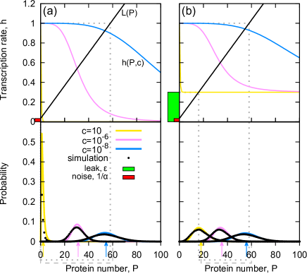
Figure 4: (Color online) Transcriptional leakage $\epsilon>1/\alpha$ narrows the range of maxima and mean values of protein distributions. (a) No leakage, $\epsilon=0$. (b) Leakage $\epsilon=0.3$. (Dotted lines) Range of maxima. (Dashed lines) Range of mean values. (Arrows) Mean values of the shown distributions. Parameters are as follows: $n=4$, $\alpha=30$, $\beta=2$.

Appendix D Mean burst frequency

Our model assumes that the promoter effectively switches between the states O and OP_n, and the switching is very fast. Transcription occurs as one of the two alternative processes (here shown for the case of repression):

$$\begin{cases}\ce{O->[k_{\mathrm{m}}]M+O}\ \ \mathrm{(with\ the\ probability\ }H(P)\mathrm{)}\\ \ce{OP_{n}->[k_{\mathrm{ml}}]M+OP_{n}}\ \ \mathrm{(with\ the\ probability\ }1-H(P)\mathrm{)}\end{cases}$$ (11)

The mean burst frequency $\nu$ for an autoregulated gene in a stationary state yields then

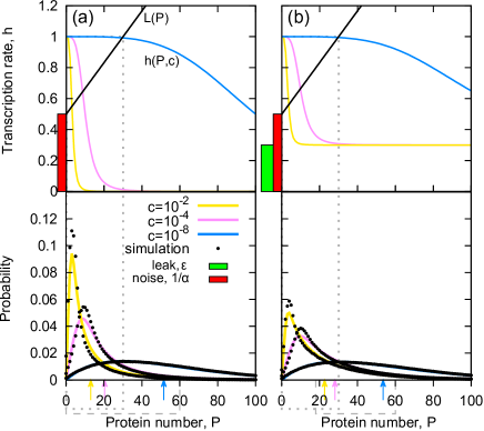
Figure 5: (Color online) When the transcriptional noise is sufficiently high, $1/\alpha>\epsilon$, the leakage does not narrow the range of maxima (dotted lines). However, the range of mean values (dashed lines) is narrower for nonzero leakage. Arrows: mean values of the shown distributions. (a) No leakage, $\epsilon=0$. (b) Leakage $\epsilon=0.3$. Parameters: $n=4$, $\alpha=2$, $\beta=30$.

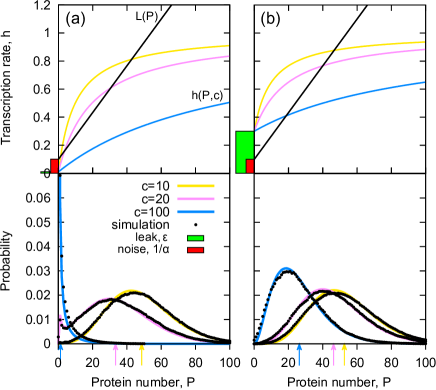
Figure 6: (Color online) (a) On the contrary to the deterministic model, binary response is possible in the stochastic model due to transcriptional bursting, even when there is just one transcription factor binding site. Here, only a very small leakage is present ($\epsilon=0.01$). (b) Transcriptional leakage ($\epsilon=0.3$) counteracts the stochastic effect of bursting by converting binary response into graded response. Parameters: $n=-1$, $\alpha=10$, $\beta=6$. Arrows: mean values of the shown distributions.

$$\nu =\frac{1}{k_{dp}}\left(k_{m}\left\langle H(P)\right\rangle_{p(P)}+k_{ml}\left\langle 1-H(P)\right\rangle_{p(P)}\right)$$ (12)

$$=\left\langle H(P)\right\rangle_{p(P)}\frac{k_{m}-k_{ml}}{k_{dp}}+\frac{k_{ml}}{k_{dp}},$$ (13)

where $p(P)$ is the protein number distribution (3), and the average

$$\left\langle H(P)\right\rangle_{p(P)}=\int_{0}^{\infty}H(P)p(P)dP$$ (14)

is used because of the assumption of a rapid switching of the promoter state. The value of (14) for a given $c$ lies between 0 and 1. Consequently, the mean burst frequency $\nu$ depends on the signal level $c$ and it lies between $k_{m}/k_{dp}$ and $k_{ml}/k_{dp}$.

We therefore interpret $\alpha=k_{m}/k_{dp}$ as the maximum mean frequency of translational bursts that can be achieved by the system. This occurs in the theoretical limit of $c=0$, i.e. when $H(P)=1$ (see Appendix B above). The parameter $1/\alpha$ is then interpreted as a measure of the minimum noise that can be achieved by the system.

Appendix E Detailed analysis of the geometric construction

(1) When the bursts are rare, $\alpha<1$, then, for both negative and positive feedback, the maximum of the protein distribution is always at $P_{max}=0$ independently of the leakage rate $\epsilon$ and the regulation strength $c$. In the deterministic model there always exist values of $c$ at which a peak occurs at $P_{max}\neq 0$. But the presence of the stochastic term $1/\alpha>1$ makes it impossible for the straight line $L(P)$ to intersect $h(P)$ for any value of $c$ (Fig. 3). Varying $c$ makes the distributions only narrower or wider, which varies the mean protein number in the range ($\alpha\beta\epsilon$, $\alpha\beta$).

(2) Negative feedback allows for graded response only. When the bursts are frequent, $\alpha>1$, there always is one intersection of $L(P)$ and $h(P)$ because of their different monotonicity. Transcriptional leakage narrows the range of regulation (Fig. 4): the maximum of $p(P)$ has the range $P_{max}\in[\max(0,\epsilon\alpha\beta-\beta);\alpha\beta-\beta]$, and the mean has the range $\langle P\rangle\in[\alpha\beta\epsilon;\alpha\beta]$. However, when the noise term $1/\alpha>\epsilon$, then the range of $P_{max}$ does not depend on $\epsilon$ (Fig. 5). Therefore, a sufficiently strong noise (long mean time between random bursts) counteracts the negative effect of leakage on the range of maxima at the cost of wider distributions (at a given $\alpha\beta$), but not on the range of mean values.

(3) When the feedback is positive and $\epsilon<1/\alpha<1$, binary response is always present because there always is a range of the signal levels in which the protein distribution is bimodal [Fig. 6A]. Note that, consistently with the results of Friedman et al. (2006), the bursting term $1/\alpha$ makes it possible to obtain binary response also for $n=-1$ [Fig. 6A], the case not predicted by the deterministic model.

(4) Transcriptional leakage counteracts the stochastic effect of bursting, by converting binary response into graded response. This is because $\epsilon>0$ shifts the base of the transfer function upwards, in such a way that, if the leakage is sufficiently large, it may enable only one intersection of $h(P)$ and $L(P)$. When the regulation is positive with $n=-1$, it suffices that the transcriptional leakage $\epsilon>1/\alpha$ to obtain graded response [Fig. 6B]. This condition is insufficient when $n<-1$. In the main text (Sec. IV), we calculated the condition for graded response in the general case of $n<0$, when $1/\alpha<1$.

Appendix F Simulation parameters

Reaction rate constants used in the mesoscopic simulations (Gillespie algorithm Gibson and Bruck (2000)) of the gene regulation kinetics have been shown in Table 2. We model the signal parameter $c$ as the ratio of effective rate constants $(k_{on,1}...k_{on,n})/(k_{off,1}...k_{off,n})$ for TF association and dissociation to the binding sites $1..n$ on the operator. The effective rates mimic the influence of the effectors or phosphorylation on the ratio of active TFs.

Figure	$k_{\mathrm{m}}$	$k_{\mathrm{ml}}$	$k_{\mathrm{dm}}$	$k_{\mathrm{p}}$	$k_{\mathrm{dp}}$	$k_{\mathrm{on}}$	$k_{\mathrm{off}}$
2.A	$3\cdot 10^{-3}$	$3\cdot 10^{-4}$	$10^{-3}$	$2\cdot 10^{-3}$	$10^{-4}$	$c=10^{3}$: {$10^{-2},5\cdot 10^{-1}$,1}; $c=2\cdot 10^{4}$: $\{10^{-3},5\cdot 10^{-2},5\}$	$\{1,5,1\}$
						$c=10^{6}$: $\{10^{-4},5\cdot 10^{-2},1\}$
2.B	$3\cdot 10^{-3}$	$9\cdot 10^{-4}$	$10^{-3}$	$2\cdot 10^{-3}$	$10^{-4}$	$c=10^{3}$: {$10^{-2},5\cdot 10^{-1}$,1}; $c=5.2\cdot 10^{4}$: $\{10^{-3},5\cdot 10^{-2},10\}$	$\{1,5,1\}$;
						$c=10^{6}$: $\{10^{-4},5\cdot 10^{-2},1\}$	$c=5.2\cdot 10^{4}$: $\{1,5,5.2\}$
S1	$0.8\cdot 10^{-4}$	$2.4\cdot 10^{-5}$	$10^{-3}$	$6\cdot 10^{-2}$	$10^{-4}$	$c=10^{-1}$: {$10^{-2},10^{-1}$}; $c=10^{-4}$: $\{10^{-2},10^{-1}\}$	$\{10^{-1},10^{-1}\}$; $\{1,10\}$
S2.A	$3\cdot 10^{-3}$	0	$10^{-3}$	$2\cdot 10^{-3}$	$10^{-4}$	$c=10$: $\{0.1,1,4,25\}$; $c=10^{-6}$: $\{0.1,1,4,25\}$$\times 10^{-7/4}$;	$\{1,1,1,1\}$
S2.B	$3\cdot 10^{-3}$	$9\cdot 10^{-4}$	$10^{-3}$	$2\cdot 10^{-3}$	$10^{-4}$	$c=10^{-8}$: $\{0.1,1,4,25\}$$\times 10^{-9/4}$
S3.A	$2\cdot 10^{-4}$	0	$10^{-3}$	$3\cdot 10^{-2}$	$10^{-4}$	$c=10^{-2}$: $\{0.01,0.1,1,10\}$; $c=10^{-4}$:	$\{1,1,1,1\}$
S3.B	$2\cdot 10^{-4}$	$6\cdot 10^{-5}$	$10^{-3}$	$3\cdot 10^{-2}$	$10^{-4}$	$\{0.1,1,10,100\}$$\times 10^{-1/2}$; $c=10^{-8}$: $\{0.1,1,10,100\}$$\times 10^{-3/2}$
S4.A	$10^{-3}$	$10^{-5}$	$10^{-3}$	$6\cdot 10^{-3}$	$10^{-4}$	10	$c=10$: 100; $c=20$: 200;
S4.B	$10^{-3}$	$0.3\cdot 10^{-3}$	$10^{-3}$	$6\cdot 10^{-3}$	$10^{-4}$		$c=100$: 1000

Table 2: Reaction rate constants used in the mesoscopic simulations of the gene regulation kinetics. Values in the curly brackets correspond to the effective rate constants of binding (or unbinding) to the consecutive binding sites.

References

- Weber and Fussenegger (2007) W. Weber and M. Fussenegger, Curr. Opin. Biotech. 18, 399 (2007).
- Minaba and Kato (2014) M. Minaba and Y. Kato, Appl. Environ. Microbiol. 80, 1718 (2014).
- Guo and Jia (2014) J. Guo and R. Jia, World J. Microbiol. and Biotechnol. 30, 1527 (2014).
- Avery (2005) S. V. Avery, Trends Microbiol. 13, 459 (2005).
- Yanai et al. (2006) I. Yanai, J. O. Korbel, S. Boue, S. K. McWeeney, P. Bork, and M. J. Lercher, Trends Genet. 22, 132 (2006).
- Dekel and Alon (2005) E. Dekel and U. Alon, Nature 436, 588 (2005).
- Shachrai et al. (2010) I. Shachrai, A. Zaslaver, U. Alon, and E. Dekel, Mol. Cell. 38, 758 (2010).
- Szekely et al. (2013) P. Szekely, H. Sheftel, A. Mayo, and U. Alon, PLoS Comput. Biol. 9, e1003163 (2013).
- Ingolia and Murray (2007) N. T. Ingolia and A. W. Murray, Curr. Biol. 17, 668 (2007).
- Rosenfeld et al. (2005) N. Rosenfeld, J. W. Young, U. Alon, P. S. Swain, and M. B. Elowitz, Science 307, 1962 (2005).
- Tabaka et al. (2008) M. Tabaka, O. Cybulski, and R. Hołyst, J. Mol. Biol. 377, 1002 (2008).
- Carey et al. (2013) L. B. Carey, D. Van Dijk, P. M. Sloot, J. A. Kaandorp, and E. Segal, PLoS Biol. 11, e1001528 (2013).
- Kringstein et al. (1998) A. M. Kringstein, F. M. Rossi, A. Hofmann, and H. M. Blau, Proc. Natl. Acad. Sci. USA 95, 13670 (1998).
- Becskei et al. (2001) A. Becskei, B. Séraphin, and L. Serrano, EMBO J 20, 2528 (2001).
- Alon (2007) U. Alon, Nat. Rev. Genet. 8, 450 (2007).
- Fraser and Kærn (2009) D. Fraser and M. Kærn, Mol. Microbiol. 71, 1333 (2009).
- Beaumont et al. (2009) H. J. Beaumont, J. Gallie, C. Kost, G. C. Ferguson, and P. B. Rainey, Nature 462, 90 (2009).
- Nevozhay et al. (2009) D. Nevozhay, R. M. Adams, K. F. Murphy, K. Josic, G. Balázsi, and K. Josić, Proc. Natl. Acad. Sci. USA 106, 5123 (2009).
- Little et al. (2013) S. C. Little, M. Tikhonov, and T. Gregor, Cell 154, 789 (2013).
- Mitrophanov et al. (2010) A. Y. Mitrophanov, T. J. Hadley, and E. a. Groisman, J. Mol. Biol. 401, 671 (2010).
- Bijlsma and Groisman (2003) J. J. Bijlsma and E. A. Groisman, Trends in microbiology 11, 359 (2003).
- Goulian (2010) M. Goulian, Curr. Opin. Microbiol. 13, 184 (2010).
- Wei et al. (2000) Z. Wei, J. F. Kim, and S. V. Beer, Mol. Plant Microbe Interact. 13, 1251 (2000).
- DiGiuseppe and Silhavy (2003) P. A. DiGiuseppe and T. J. Silhavy, J. Bacteriol. 185, 2432 (2003).
- Stachel and Zambryski (1986) S. E. Stachel and P. C. Zambryski, Cell 46, 325 (1986).
- Yamamoto et al. (1987) A. Yamamoto, M. Iwahashi, M. F. Yanofsky, E. W. Nester, I. Takebe, and Y. Machida, Mol. Gen. Genet. 206, 174 (1987).
- Friedman et al. (2006) N. Friedman, L. Cai, and X. Xie, Phys. Rev. Lett. 97, 168302 (2006).
- Koch and Levy (1955) A. L. Koch and H. R. Levy, J. of Biol. Chem. 217, 947 (1955).
- Taniguchi et al. (2010) Y. Taniguchi, P. J. Choi, G.-W. Li, H. Chen, M. Babu, J. Hearn, A. Emili, and X. S. Xie, Science 329, 533 (2010).
- Geisberg et al. (2014) J. V. Geisberg, Z. Moqtaderi, X. Fan, F. Ozsolak, and K. Struhl, Cell 156, 812 (2014).
- Munchel et al. (2011) S. E. Munchel, R. K. Shultzaberger, N. Takizawa, and K. Weis, Molecular biology of the cell 22, 2787 (2011).
- Belle et al. (2006) A. Belle, A. Tanay, L. Bitincka, R. Shamir, and E. K. O’Shea, Proceedings of the National Academy of Sciences 103, 13004 (2006).
- Shahrezaei and Swain (2008) V. Shahrezaei and P. Swain, Proc. Natl. Acad. Sci. USA 105, 17256 (2008).
- Ochab-Marcinek and Tabaka (2010) A. Ochab-Marcinek and M. Tabaka, Proc. Natl. Acad. Sci. USA 107, 22096 (2010).
- Mackey et al. (2010) M. C. Mackey, M. Tyran-Kamińska, and R. Yvinec, J. Theor. Biol. 274, 84 (2010).
- Aquino et al. (2012) T. Aquino, E. Abranches, and A. Nunes, Phys. Rev. E 85, 061913 (2012).
- Horsthemke and Lefever (1984) W. Horsthemke and R. Lefever, Noise-induced transitions: theory and applications in physics, chemistry, and biology (Springer Verlag, 1984).
- Gibson and Bruck (2000) M. A. Gibson and J. Bruck, J. Phys. Chem. A 104, 1876 (2000).