Gravitational waves in bigravity cosmology
Abstract
In this paper we study gravitational wave perturbations in a cosmological setting of bigravity which can reproduce the CDM background and large scale structure. We show that in general gravitational wave perturbations are unstable and only for very fine tuned initial conditions such a cosmology is viable. We quantify this fine tuning. We argue that similar fine tuning is also required in the scalar sector in order to prevent the tensor instability to be induced by second order scalar perturbations. Finally, we show that due to this power law instability, models of bigravity can lead to a large tensor to scalar ratio even for low scale inflation.
pacs:
04.50.Kd, 11.10.EfI Introduction
The problem of dark energy is one of the fundamental problems not only of cosmology but of theoretical physics. How can vacuum energy, or equivalently a cosmological constant, be as small as the measured density of dark energy? (Fine tuning problem.) And why should it be of the same order of magnitude as the present mean density of matter in the Universe? (Coincidence problem.) These questions have led cosmologists to search for alternative explanations of the accelerated expansion of the Universe.
The possibility of giving the graviton a mass has attracted considerable attention. Such a mass leads to ‘degravitation’ which can solve the cosmological constant problem Dvali:2007kt ; deRham:2007rw ; deRham:2009rm . If the graviton is massive, the range of gravity is finite and a cosmological constant does not gravitate. Furthermore, if one fine tunes the graviton mass to , where GeV is the value of the Hubble constant and km/sec/Mpc, gravity weakens around this scale, which might lead to accelerated expansion.
Adding a mass term to gravity is a non-trivial problem. It removes diffeomorphism invariance and hence the metric has six degrees of freedom (four being absorbed by the Bianchi identities). Five of these are the massive graviton while the sixth is usually a ghost, the so-called Boulware-Deser ghost Boulware:1973my . To remove this ghost one has to make sure to obtain an additional constraint. This was shown to be possible with a very specific form of the potential for the gravitational field, the dRGT (de Rham, Gabadadze, Tolley) potential deRham:2010ik ; deRham:2010kj ; Hassan:2011hr , which has been the basis for a large amount of work on this topic (see, e.g., Hassan:2011vm ; Hassan:2011tf ; Koyama:2011yg ; Guarato:2013gba and refs. therein). Applications to cosmology, however, have shown that it is not possible to find homogeneous and isotropic solutions of massive gravity which resemble our Universe. In massive gravity, a fixed reference metric has to be chosen with respect to which the mass term is defined. The possible solutions of course strongly depend on this reference metric, but even when choosing the reference metric to be Friedmann, the resulting solutions either do not show the well known cosmological behavior going from a radiation dominated to a matter dominated Universe followed by a late dark energy dominated phase, or they are unstable Gumrukcuoglu:2011zh ; Langlois:2012hk ; Fasiello:2012rw , see deRham:2014zqa for a review and Comelli:2013tja ; deRham:2014gla for the study of the cosmology in the contest of the so-called generalized massive gravity models.
Apart from these problems, it is somewhat disappointing to introduce the reference metric as an ‘absolute element’, i.e., a non-dynamical field in the theory. From this point of view, bimetric (or more general multi-metric) theories, where also the reference metric is dynamical are better motivated Hassan:2011zd ; Hassan:2011ea ; Hassan:2012wr . Interesting discussions about theoretical aspects of bimetric massive gravity can be found in Akrami:2014lja ; Hassan:2014vja ; deRham:2014fha ; Cusin:2014zoa ; Noller:2014sta ; Akrami:2013ffa .
It has been shown that bigravity theories can by stable and well behaved Fasiello:2013woa , and that cosmological solutions of bimetric theories can actually fit the expansion history of the accelerating Universe Volkov:2011an ; Comelli:2011zm ; Konnig:2014dna ; Tamanini:2013xia . Observational tests of various models of bigravity are discussed in Solomon:2014dua ; vonStrauss:2011mq ; Berg:2012kn ; 2013JHEP…03..099A ; Konnig:2013gxa . The study of the cosmology of models of bigravity where matter is coupled to a combination of the two metrics is addressed in a series of recent papers Gumrukcuoglu:2015nua ; Comelli:2015pua ; Enander:2014xga . The analysis of cosmological perturbations have been studied in different settings and different models of bigravity in Comelli:2012db ; Comelli:2014bqa ; DeFelice . Recently, scalar perturbations of these models have been investigated and it has been shown that there exists a sub-class of models of bigravity that admit solutions with well behaved scalar perturbations of the physical metric, while other sub-classes of models are unstable Amendola_pert .
In this paper we want to study the behavior of tensor perturbations, i.e., gravitational waves in bimetric gravity theories which fit the expansion history of the Universe and which lead to physically acceptable scalar perturbations, i.e., scalar perturbations which just exhibit the usual Jeans instability of Newtonian gravity which leads to cosmological structure formation but no significant additional instability. A more generic study of instabilities in bimetric theories can be found in Ref. Kuhnel:2012gh .
Examining cosmological tensor perturbations, we show that gravitational waves are unstable in this theory. We study this instability in detail. We find that it changes the spectrum and strongly boosts the amplitude of gravitational waves. In order to prevent conflict with observations we have to fine tune the initial conditions for tensor perturbations.
While we were working on this, a preliminary study of gravitational waves in this model has appeared Lagos:2014lca . In Ref. Lagos:2014lca the authors investigate all perturbation modes, scalar, vector and tensor for two cosmological solutions, namely the expanding branch and the bouncing branch, called infinite-branch bigravity (IBB) in Ref. Amendola_pert . This latter has cosmologically acceptable scalar perturbations and is therefore of particular interest.
Our analysis goes beyond the results presented in Lagos:2014lca . We numerically solve the gravitational wave equations and study the resulting gravitational wave spectrum for different initial conditions for the perturbations. We finally argue that even if we would initially set gravitational wave perturbations to zero, non-linearities which induce small tensor perturbations are sufficient to trigger the instability and the model can only be saved if we also fine tune the initial conditions of scalar perturbations.
The rest of the paper is organised as follows. In the next section we write the Lagrangian and the equations of motion of bimetric gravity in general and for cosmological (i.e. homogeneous and isotropic) spacetimes. We then specialise to the physically viable model which gives an acceptable expansion history. In Section III we comment on the scalar sector of perturbations and in Section IV we study tensor perturbations and compute the gravitational wave spectrum for different initial conditions. In Section V we discuss our results and conclude.
Notation: We set . GeV is the reduced Planck mass.
II Cosmological solutions of massive bigravity
II.1 The Lagrangian
We start from a massive bigravity theory defined by the action
| (1) |
Here and are the two metrics while and are the respective Planck masses with dimensionless ratio . We assume the matter fields to be coupled to only. We use the notation of vonStrauss:2011mq . The potential is a function of the tensor field given by
| (2) |
where the polynomials are
| (3) | |||||
| (4) | |||||
| (5) | |||||
| (6) |
The square bracket denotes the trace. The equations of motion of this theory are
| (7) | |||||
| (8) |
where the superscript indicates the curvature of the metric . The definition of the matrices and is as follows
As a consequence of the Bianchi identities and of the covariant conservation of , we obtain the following Bianchi constraints for each of the two metrics
| (9) |
| (10) |
where we raise and lower indices of and with the metrics and respectively and the relevant metric is indicated in the covariant derivatives and . Both these constraints follow from the invariance of the interaction term under the diagonal subgroup of the general coordinate transformations of both metrics. Both constraints are equivalent and we will use only the first one.
II.2 Cosmological equations of motion
We now consider solutions which are spatially homogeneous and isotropic. For simplicity we neglect spatial curvature. If curvature is included, it is easy to see that it has to be the same for both metrics. The metrics can be written in the form
| (11) |
| (12) |
where is conformal time for the -metric and is a lapse function which parametrizes the difference between the conformal time for the -metric and , .
It is convenient to define the conformal Hubble parameter () and the standard one () for the two metrics
| (13) |
where with ′ we denote the derivative with respect to the conformal time . We also introduce the ratio between the two scale factors
| (14) |
For symmetry reasons, the energy-momentum tensor has the form of a perfect fluid with equation of state . Explicitly
| (15) | |||||
| (16) | |||||
| (17) |
Introducing a ‘gravity fluid’ which represents the mass term in the Einstein equations, we define
| (18) | |||||
| (19) |
Note that the gravity fluid becomes like a cosmological constant when .
The Bianchi constraint in the cosmological ansatz can then be written as
| (20) |
This constraint is equivalent to
| (21) |
The full set of equations of motion is given by the time-time and the space-space components of the modified Einstein equations. For the metric they are
| (22) |
| (23) |
The modified Friedmann equations for the metric become
| (24) | |||||
| (25) |
We consider the first Friedmann equation for both metrics, the Bianchi constraint, and in the matter sector, the ‘energy conservation’ equation and the equation of state as independent equations which determine the 5 functions , , , and ,
| (26) |
| (27) |
| (28) |
| (29) |
Eq. (28) allows for two branches of solutions. Either is constant given by the solution of the quadratic equation
| (30) |
or the second factor of eq. (28) vanishes implying
| (31) |
According to vonStrauss:2011mq ; DeFelice the first branch is equivalent to general relativity with an effective cosmological constant. Therefore we expect the usual CDM phenomenology for this branch. We now concentrate on the second branch which is more interesting, hence we request . Inserting this in (27) yields
| (32) |
With this, the Friedmann equation for can be written as
| (33) |
This is a polynomial equation which can be solved for in terms of the energy density and the constants , , and . The detailed evolution depends on the parameters but we can already observe that at late time, when , const so that also const. Therefore we have a late-time de Sitter phase, independent of the choice of parameters, as long as these admit a real and positive solution of the fourth order equation given by (33) with .
A detailed study of the background cosmology in this cosmological setting can be found in Comelli:2011zm ; Konnig:2013gxa . Several possible branches of the solutions are possible, depending on the initial values for . In Konnig:2013gxa , a series of conditions defining a viable cosmological evolution are elaborated. Violations of these conditions do not necessarily imply contradiction with observations if they occur outside the observable range, hence in principle they can be relaxed or lifted. However, when these conditions are satisfied, the cosmological evolution requires no special tuning and it is much safer.
In order not to mimic a cosmological constant we set . We now study in detail the case (we call it the ‘- model’) which has been identified as the only one which gives both, an acceptable background solution and viable scalar perturbations Konnig:2013gxa ; Arkami:2013a1 ; Amendola_pert .
We consider a Universe containing matter and radiation with densities and and pressure and which we assume to be separately conserved such that and . Here we have normalized the scale factor to unity today, . The Bianchi constraint can be rewritten as
| (34) |
Furthermore, under the rescaling and the equations become independent of so that we can simply set , see Berg:2012kn for a more detailed discussion. With this, the background equations can be written as
| (35) |
| (36) |
| (37) |
We solve the first three equations for , and ,
| (38) |
| (39) |
| (40) |
We want to solve eq. (40) numerically for a given present value of . Let us divide eq. (38) by so that
| (41) |
We now evaluate eq. (41) at and we solve the resulting equation expressing as a function of the constants . This equation has three real solutions. We choose the only one that, when used as ‘final’ condition in eq. (40), gives an evolution for starting at very large values and decreasing to a finite value at late times. In Konnig:2013gxa and Amendola_pert , it has been shown that this solution is the only one able to give rise to both a viable background cosmology and viable scalar perturbations in the - model.
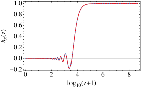
We choose the best-fit values and obtained in Konnig:2013gxa and Amendola_pert fitting measured growth data and type Ia supernovae (see also Arkami:2013a1 for an explanation of the procedure used to obtain these values from fits). We can then solve eq. (40) numerically. The evolution of is shown in Fig. 1.
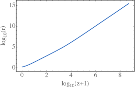
We observe that is very large at early times (the vertical axis is not but ), at the present time while the value is a future attractor.
The lapse of the -metric is given by the Bianchi constraint (34). Its time evolution is presented in Fig. 2.
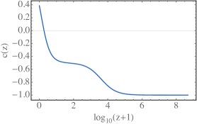
The lapse function is constant in the radiation dominated phase, so that , hence , see Eq. (34). It grows to a new plateau at the matter-radiation transition and stays during the matter dominated phase. Then again at the transition to the gravity-dominated phase in the future, the lapse grows to which is reached in the future de Sitter phase. Interestingly, the lapse function changes sign roughly at redshift . This in principle signals a singularity in the -metric where, for example, its determinant vanishes. However, since the Bianchi constraint requires that also when and , remains finite and no physical observable diverges111This would be different if we would couple matter to the -metric since e.g. its Ricci scalar which might then become observable diverges..
At this point we want to direct the attention of the reader to the fact that even though in the Langrangian the lapse function only appears as which one naively might replace by , this cannot lead to the background phenomenology needed to mimic dark energy. At early times, when and the Universe is radiation dominated, Eq. (40) becomes
| (42) |
For the second equal sign we have used Eq. (38) in the limit of large . In order to satisfy both, Eq. (34) and Eq. (40), we therefore need in the radiation dominated era and we cannot replace by in Eq. (34). We can also not replace it by since we need the factor when the Universe becomes dark energy dominated. With our choice of the parameters , a radiation dominated Universe at early time and a dark energy like solution at late time, requires that passes through zero, which cannot.
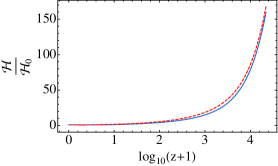
Substituting the numerical solution for in eq. (41), we obtain the evolution of . In Fig. 3 we have plotted as a function of redshift in - bigravity and in standard .222We have considered a scenario with radiation, matter and a cosmological constant with .

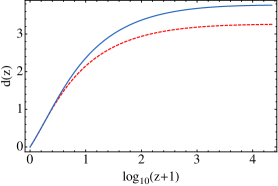
In Fig. 4 we compare the background evolution of the comoving distance for the - model with the best fit parameters , (which we shall also consider in the perturbation analysis) and for a CDM model with .
III Comments on scalar perturbations
Let us now consider perturbations of this cosmology around the homogeneous and isotropic background
| (43) |
| (44) |
From now on, the use of an overbar indicates background quantities. We parametrize the perturbations as follows
| (45) |
| (46) |
with
| (47) |
Spatial indices are raised and lowered using the flat spatial metric, . There are eight scalar perturbations, and , eight vector perturbations, and and four tensor perturbations . Here ∙ denotes g or f. Two scalar and two vector modes can be removed by coordinate transformations, leaving six scalar, six vector and four tensor degrees of freedom.
In Ref. Amendola_pert scalar perturbations of the viable - model have been analysed for perfect fluid matter (i.e. matter without anisotropic stress and with adiabatic perturbations) and it has been found that they can fit the growth rate of the observed perturbations during the matter and dark energy dominated eras333One of the main conclusions of Ref. Amendola_pert is that during matter domination scalar perturbations do not exhibit exponential instabilities. In that context, however, the stability of scalar perturbations at early times and the absence of power-low instabilities during matter is not analysed.. In Ref. Lagos:2014lca a preliminary analysis of all, scalar, vector and tensor perturbations is presented and analytic solutions in limiting regimes are found, which all do not show exponential instabilities.
In this section we discuss briefly scalar perturbations while the rest of this work is devoted to a detailed study of tensor perturbations. For the scalar sector, we derive analytic solutions for the propagating degrees of freedom valid in the radiation era and we compare them with the results of the numerical integration of the perturbation equations in radiation. The result of this analysis differs from the one of Ref. Lagos:2014lca and we find that an instability in the scalar sector of the metric shows up at early times and, if sufficiently large, it is transferred to the physical sector of the metric through the coupling between the two sectors.
The equations for the two propagating scalar degrees of freedom in the radiation dominated era can be approximated by 444We adopt here the gauge choice of Ref. Lagos:2014lca to eliminate the redundant degrees of freedom in the scalar sector.
| (48) |
| (49) |
For super-Hubble modes, , we can neglect terms proportional to . Furthermore, in the background branch under study, in the radiation era we have , and constant. Hence, in this regime, the last three terms in (48) and (49) can be dropped and the two equations decouple.
The solutions of the resulting approximated equations can be written as 555More precisely, the exact solution of the decoupled eq. (49) has a constant mode and a growing one proportional to . This function is growing roughly like as long as the argument is smaller than , hence during the entire radiation dominated epoch. It can therefore be approximated with the growing mode in (50) to good precision.
| (50) |

In the physical sector we recover the usual behavior of super-Hubble scalar perturbation in the radiation dominated era, while the perturbations of grow linearly. Neglecting the constant mode for and the subdominant decaying mode for , we have
| (51) |
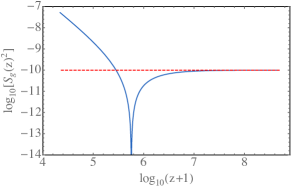
We solve Eqs. (48) and (49) numerically with initial conditions (51) and we compare the result with the analytical solution valid in the radiation era, see Fig. 5. The analytical and numerical solutions for are in very good agreement. The solution for , however is soon affected by the coupling term in (48) which can be large for small values of .
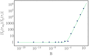
We then choose the initial condition for scalar perturbations in the physical sector compatible with the observational constraints from structure formation, , and we explore how the evolution changes varying , i.e., the initial condition for , see Fig. 6. If the ratio between the initial condition of and is big, i.e. , the solution for develops a growing mode in the radiation dominated epoch. In Fig. 7 we plot the amplification of at the end of the radiation era () as a function of . We see that the amplification is roughly proportional to the initial condition of for . The amplification during the radiation era is absent for .
Comparing the order of magnitude of the terms in eq. (48) we find in order for the instability to develop during the radiation dominated era we need
| (52) |
For a realistic value of and our example plotted in Fig. 6, i.e., , this requires . For an early inflationary phase with reheat temperature GeV we obtain , hence in order to avoid this mild instability we need to require that
| (53) |
Hence for early inflation, only very fine tuned initial condition can avoid to be affected by this instability in the scalar sector.
IV Gravitational waves in massive bigravity cosmology
Tensor perturbations of a given -mode can be written as
| (54) |
where and denote the two helicity-2 modes of the gravitational wave. For an orthonormal system we have
| (55) |
For parity invariant perturbations
and . This is what we shall assume in the following and we shall consider just one mode, say and . Here is a Gaussian random variable with vanishing mean and with variance , so that is the square root of the power spectrum. All what follows is also valid for the modes which are not correlated with in the parity symmetric situation which we consider.
For the first order modified Einstein equation with a perfect fluid source term, i.e. no anisotropic stress, we obtain the following tensor perturbation equations for our bimetric cosmology
| (56) |
| (57) |
At very early times, in the radiation dominated Universe where we want to define our initial conditions, is very large and constant. Furthermore, constant. This implies that in this limit the square bracket of eq. (57) becomes and the coupling term is suppressed by a factor with respect to the coupling term in eq. (56) and can be neglected. Choosing a super Hubble mode, and recalling that in the radiation era , we can neglect the term proportional to in both the equations. To be consistent, in eq. (56), we then have to neglect also the coupling term, since for the best fit parameters with . On super Hubble scales in the radiation era we then obtain the solutions
| (58) | |||||
| (59) |
The solution for differs from the one found in Ref. Lagos:2014lca : in this work when deriving the approximated equation valid in the radiation era for super Hubble modes, the term proportional to in eq. (58) is not neglected. As explained above, this approximation is not completely consistent.666This can be checked substituting the solutions found in Ref. Lagos:2014lca with coefficients expressed as functions of the initial conditions after inflation in the full equations for perturbations: the terms which do not cancel are negligible only in the specific case in which the initial condition for after inflation is fine-tuned to be very small, .
Interestingly, when neglecting the coupling term which for is never relevant, the first expression for the solution (59) is valid both in the radiation and matter era on all scales as long as constant. Actually, in the matter dominated era the anti-damping term in eq. (57) becomes and with , the equation remains unchanged. The functions and denote the spherical Bessel functions Abramo and in the radiation era while in the matter era. Considering the growing mode proportional to we find that grows like on super Hubble scales and like on sub Hubble scales.
However, in general we can no longer neglect the coupling term in the solution for since, depending on the initial condition may have grown too large to be neglected in its coupling to . In contrary, since cannot grow more than and since the pre factor of the coupling term remains small, the coupling can be neglected in the equation and (59) remains a good approximation on super Hubble scales.
The solution for in the radiation dominated era agrees with the well know GR solution, but has a growing mode which indicates the presence of an instability. Neglecting the decaying modes we choose the initial conditions
| (60) |
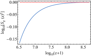
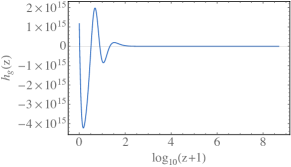
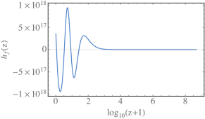
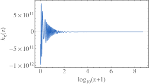
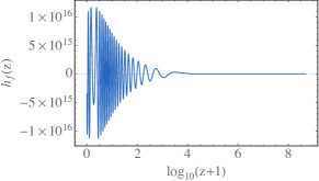
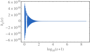
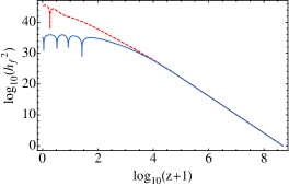
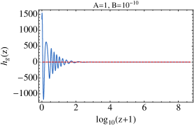
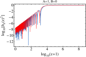
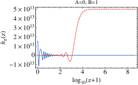
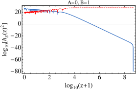
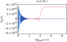
The behaviour of the solution depends very sensitively on the initial condition, in the following we explore different possibilities. Naively, we might argue that initially, e.g., after inflation, both and are of the same order of magnitude, . The gravitational waves and for these initial conditions found by solving numerically Eqs. (56) and (57) for the wave numbers are shown in Fig. 8. In a linear plot it looks as if and would be nearly constant during radiation, then starts oscillating with frequency and with increasing amplitude at redshift corresponding to the horizon crossing for the mode chosen. The instability is transferred to the mode trough the coupling. In Fig. 9 we present a log-plot for the same modes together with the analytic solutions (58,59). The analytic solution for is a very good approximation on super-Hubble scales. There one sees that the growth on super Hubble scales turns into the milder growth after Hubble entry.

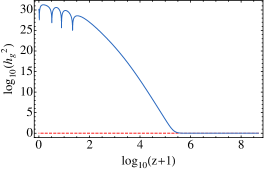

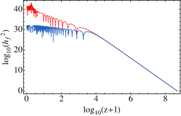
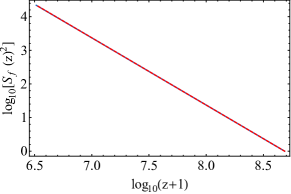
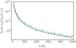
When , the gravitational wave amplitude today is amplified tremendously, for a mode with wavenumber , roughly by a factor , as shown in Fig. 10. Therefore, in any case, if the initial amplitudes are not very small, gravitational wave perturbations will grow very large at late time.
.
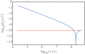
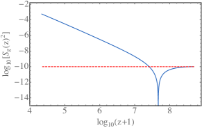
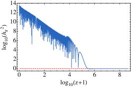
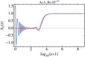
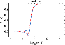
We want to check whether there exists a choice of the initial conditions such that we recover an evolution of tensor perturbations similar to the one of and an amplitude of tensor perturbations today which is of order of the one of . We find that if we tune the initial conditions for to be very small, i.e. , the instability can be avoided and we can recover an evolution of tensor perturbations at late times (i.e. during the matter era and later) that is similar to the standard gravitational wave evolution of General Relativity. In Fig. 11 we show how the evolution of tensor perturbations is affected by decreasing . The evolution of tensor perturbation in the bigravity model for different initial values at fixed is superimposed to the result with initial condition , .
The amplitude of at late times is proportional to for values of . For smaller values of it converges to the GR result and becomes independent of . In other words, if is not about 16 orders of magnitude smaller than initially, the value of the latter at late times is entirely determined by .
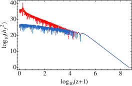
The small shift in redshift of the bimetric spectrum for with respect to the one of is due to the presence of a slight difference between the evolution of the scale factor in the - bigravity model compared to (see Fig. 3), while the coupling of the tensor mode with in the perturbation equation (56) is effectively negligible. This can be checked easily comparing the spectrum of tensor perturbations of the bigravity model with the one of , calculated on a bigravity background: the two spectra overlap with a very good precision777In other words, if we choose fine-tuned initial conditions for tensor perturbations, , the coupling between the two tensor modes in (56) is effectively negligible and the fact that the evolution of tensor perturbations of the physical metric differs form the one in can be simply ascribed to a slightly different background evolution. , as shown in Fig. 13.


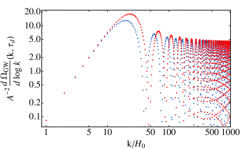
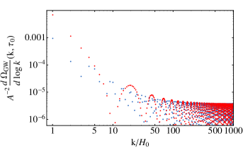
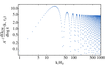
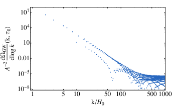
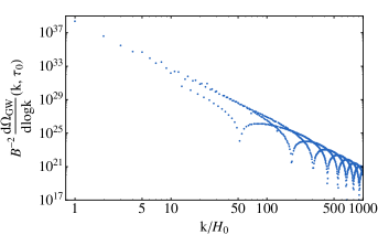
In Fig. 14 we show the energy spectrum of the gravitational waves in units of the critical density
| (61) |
for the cases and and at the redshift of decoupling and today.

Let us also make the following remark: one might worry about the singularity of the term in eq. (28) when the lapse function of the metric, , passes through zero (see Fig. 2). It can actually be shown by a simple analytic argument that this singularity is just an apparent one. First, by using eq. (34), we find that eq. (57) can also be written as
| (62) |
When , eq. (62) can be approximated by
| (63) |
which is solved by . Therefore the singularity in the term in eq. (63) when is cancelled by the factor and the differential equation for is regular for all values of . The fact that passes through zero when at is well visible in Fig. 15.

V Discussion and conclusions
V.1 Higuchi bounds
In cosmology and in particular in theories of modified gravity, it is important to check whether the theory may contain ’ghosts’. In this context a ghost is a degree of freedom with a kinetic term of the wrong sign. The energy of such a degree of freedom is not bounded from below and via its coupling to other degrees of freedom it can pass to them unlimited amounts of energy, rendering the theory unstable and therefore unphysical. In a static spacetime this instability is exponential. In an expanding spacetime it is typically a milder power law instability.
As pointed out for the first time by Higuchi Higuchi:1986py , even though the sixth degree of freedom of generic massive gravity, which is always a ghost, is absent, in the dRGT theory of massive gravity the helicity-0 mode of the massive graviton can behave like a ghost for particular values of the theory on a de Sitter background, leading to instabilities of the theory beyond the classical linear regime. The condition for having the kinetic term positive definite is known as Higuchi bound. The study of the stability of massive gravity linearized around a de Sitter background (with flat reference metric) was continued in Woodard where it has been shown that the helicities ( and ) of the massive graviton are stable and unitary since they are immune to the helicity-0 constraint.
The requirement that the helicity-0 mode on a FRW background has a positive-definite kinetic term is referred to as the generalized Higuchi bound. This has been studied for the first time in the bigravity theory in Fasiello:2012rw and in Fasiello:2013woa (see also DeFelice for an alternative analysis of the scalar sector).
In the background branch with , the generalised Higuchi bound for the helicity-0 mode can be written as
| (64) |
where
| (65) |
For the vector modes we find instead the condition
| (66) |
which is always satisfied in the - model. This is not the case for the Higuchi bound for the helicity-0 mode as has been noted also in Ref. Lagos:2014lca . Indeed, using the background constraints, eqs. (35-37), the bound (64) can be written as
| (67) |
For the best-fit values with , this constraint is satisfied only in the asymptotically de Sitter phase of the cosmological expansion, where so that the bound is saturated. Hence, the scalar sector is affected by a ghost instability. In an expanding Universe with time dependent Hubble parameter, this instability is not exponential like in the de Sitter case but it manifests itself by the presence of a power law growing mode in the scalar sector of perturbations, as found in Sec. III.
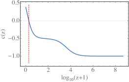
In the context of bigravity, the Higuchi bound in the tensor sector has not been properly addressed in the literature. If we write the quadratic kinetic part of the action for the tensor modes from eq. (1), we find
| (68) |
where comes from the square root of the determinant of the -metric. Here we can choose either or for , but we are not allowed to choose in order to have a differentiable action 888For a detailed discussion of this point, see also Refs. Gratia:2013gka ; Gratia:2013uza .. To reproduce the phenomenology discussed in this paper we have to choose the positive square root999We could also choose , but then we would have to change the sign of to reproduce the CDM phenomenology, so that in the end it does not change our finding that there is a ghost in the tensor sector.. Only with this we obtain the correct equations of motion, e.g. eq. (34). Therefore the correct action is
| (69) |
and the kinetic term for the tensor mode of the metric is positive definite only if .
In the background branch that we consider, is negative and crosses zero at recent time, . This means that along the entire cosmological evolution, the helicity-2 sector is affected by a ghost instability. This instability is connected with the one we have observed in the study of perturbations. Actually, writing the -equation in the form (62) shows that in the epochs of constant, the sign of indicates whether we have a damped () or anti-damped () evolution. At late time, the lapse function changes sign and the tensor sector becomes healthy. This is clearly visible in the numerical solutions shown in Fig. 8 where one sees a decay of the amplitude of at very late times.
The physical interpretation to the negative sign of the lapse is that the time for the -metric sector goes in the opposite direction with respect to the time for the physical sector. The scale factor is decreasing when is increasing since . As a consequence, instead of decreasing, the amplitude of tensor perturbations for the -metric are growing in time.
We have chosen the lapse negative at early times and crossing zero going to positive value only at very recent times. We observe that we could have done the opposite choice, taking at early times. This choice however does not give rise to a viable cosmological evolution.
Finally, we stress that a violation of the generalized Higuchi bound in a Friedmann universe is not as devastating as it is in a de Sitter universe since the instability it gives rise to is power law and not exponential. Nevertheless, in order to agree with observations which are well reproduced with the GR behaviour, we need to fine tune these unstable modes so that their initial conditions are significantly suppressed compared to the usual GR modes.
V.2 Non-linearities
There is an additional subtlety which becomes relevant as soon as there are unstable modes in a theory which is intrinsically non-linear. It is a simple choice of initial conditions to set the unstable modes to zero initially and within linear perturbation theory we have found that their coupling to the other modes is sufficiently suppressed so that they are not generated significantly.
However, once we go beyond linear perturbation theory it is to be expected that the unstabler modes should acquire amplitudes of the order of where is a typical linear mode which we expect to couple to all other modes at the next order. Therefore, even if a given inflationary model does not generate any tensor perturbations we expect tensor perturbations induced from scalar perturbations on the level of . For the case of general relativity these induced perturbations have been calculated in 2nd order perturbation theory and numerically Ananda:2006af ; Adamek:2014xba .
However, the coupling of the -metric to the -metric is suppressed by a factor which makes it very small. As we have seen, at least at linear order the coupling of the -metric to -perturbations is nearly always negligible. Therefore, an inflationary model with nearly vanishing initial conditions for the -metric may actually remain viable.
V.3 Conclusions
We have found that in bimetric cosmology the tensor perturbations of the second metric, the one that does not couple to matter, exhibits a power law instability, on super Hubble scales and on sub Hubble scales. For ‘natural’ initial conditions with , the time evolution of is very different from the behavior in CDM cosmology. Due to its coupling to it grows rapidly and the final gravitational wave spectrum is determined entirely by the initial amplitude of . Only if the initial amplitude of is suppressed by a factor of about w.r.t we can recover the standard behavior of gravitational waves. This opens up new possibilities to test bimetric cosmology via the gravitational wave sector. Not only the final gravitational wave spectrum shown in Figs. 14(a) to 14(f) can be very different from the standard GR result, but also its time evolution differs leading to a different signature in the CMB.
To determine the initial conditions and we would have to specify an inflationary phase which generates them. Assuming an agnostic point of view as we have done in this work, no firm predictions can be made. Nevertheless, if inflation reheats to about GeV, the gravitational wave amplitude on very large scales at late times is of the order of unless . In other words, unless there is a very significant suppression of gravitational waves of the -metric, their amplitude and time evolution will completely dominate the gravitational wave signal and show up in the CMB.
This finding has yet another consequence: we may obtain a significant gravitational wave signal even from low energy inflation. For an inflationary Hubble parameter , the gravitational wave amplitude is typically , leading to a tensor to scalar ratio . Assuming a bimetric theory with we now obtain a scalar to tensor ratio from inflation given by
| (70) |
Since the scalar perturbation amplitude is
this requires
For standard inflation requires for a tensor to scalar ratio of .
Setting we obtain for our bimetric cosmology
| (71) |
For arbitrary values of we obtain correspondingly
| (72) |
This rules out all simple well motivated inflationary models which cannot provide a mechanism to suppress the generation of -perturbations during inflation.
To conclude, we have found that both, the scalar and the tensor sectors of - bimetric theories, exhibit a power law instability which is related to the Higuchi ghost. Depending on the inflationary model, this instability can render the theory in serious conflict with observation. On the other hand, it may also open a new possibility to obtain significant tensor perturbations from low scale inflation.
Acknowledgments
We thank Julian Adamek, Jens Chluba, Yves Dirian, Stefano Foffa, Michele Maggiore and Ignacy Sawicki for interesting discussions and suggestions. This work is supported by the Swiss National Science Foundation.
References
- (1) G. Dvali, S. Hofmann, and J. Khoury, “Degravitation of the cosmological constant and graviton width,” Phys.Rev. D76 (2007) 084006, arXiv:hep-th/0703027.
- (2) C. de Rham, S. Hofmann, J. Khoury, and A. J. Tolley, “Cascading Gravity and Degravitation,” JCAP 0802 (2008) 011, arXiv:0712.2821.
- (3) C. de Rham, “Massive gravity from Dirichlet boundary conditions,” Phys.Lett. B688 (2010) 137–141, arXiv:0910.5474.
- (4) D. Boulware and S. Deser, “Can gravitation have a finite range?,” Phys.Rev. D6 (1972) 3368–3382.
- (5) C. de Rham and G. Gabadadze, “Generalization of the Fierz-Pauli Action,” Phys.Rev. D82 (2010) 044020, arXiv:1007.0443.
- (6) C. de Rham, G. Gabadadze, and A. J. Tolley, “Resummation of Massive Gravity,” Phys.Rev.Lett. 106 (2011) 231101, 1011.1232.
- (7) S. Hassan and R. A. Rosen, “Resolving the Ghost Problem in non-Linear Massive Gravity,” Phys.Rev.Lett. 108 (2012) 041101, 1106.3344.
- (8) S. Hassan and R. A. Rosen, “On Non-Linear Actions for Massive Gravity,” JHEP 1107 (2011) 009, 1103.6055.
- (9) S. Hassan, R. A. Rosen, and A. Schmidt-May, “Ghost-free Massive Gravity with a General Reference Metric,” JHEP 1202 (2012) 026, 1109.3230.
- (10) K. Koyama, G. Niz, and G. Tasinato, “Strong interactions and exact solutions in non-linear massive gravity,” Phys.Rev. D84 (2011) 064033, 1104.2143.
- (11) P. Guarato and R. Durrer, “Perturbations for massive gravity theories,” Phys.Rev. D89 (2014) 084016, 1309.2245.
- (12) A. E. Gumrukcuoglu, C. Lin, and S. Mukohyama, “Cosmological perturbations of self-accelerating universe in nonlinear massive gravity,” JCAP 1203 (2012) 006, 1111.4107.
- (13) D. Langlois and A. Naruko, “Cosmological solutions of massive gravity on de Sitter,” Class.Quant.Grav. 29 (2012) 202001, arXiv:1206.6810.
- (14) M. Fasiello and A. J. Tolley, “Cosmological perturbations in Massive Gravity and the Higuchi bound,” JCAP 1211 (2012) 035, arXiv:1206.3852.
- (15) C. de Rham, “Massive Gravity,” 1401.4173.
- (16) D. Comelli, F. Nesti, and L. Pilo, “Cosmology in General Massive Gravity Theories,” JCAP 1405 (2014) 036, 1307.8329.
- (17) C. de Rham, M. Fasiello, and A. J. Tolley, “Stable FLRW solutions in Generalized Massive Gravity,” 1410.0960.
- (18) S. Hassan and R. A. Rosen, “Bimetric Gravity from Ghost-free Massive Gravity,” JHEP 1202 (2012) 126, 1109.3515.
- (19) S. Hassan and R. A. Rosen, “Confirmation of the Secondary Constraint and Absence of Ghost in Massive Gravity and Bimetric Gravity,” JHEP 1204 (2012) 123, 1111.2070.
- (20) S. Hassan, A. Schmidt-May, and M. von Strauss, “On Consistent Theories of Massive Spin-2 Fields Coupled to Gravity,” JHEP 1305 (2013) 086, 1208.1515.
- (21) Y. Akrami, T. S. Koivisto, and A. R. Solomon, “The nature of spacetime in bigravity: two metrics or none?,” Gen.Rel.Grav. 47 (2015), no. 1 1838, 1404.0006.
- (22) S. Hassan, A. Schmidt-May, and M. von Strauss, “Particular Solutions in Bimetric Theory and Their Implications,” 1407.2772.
- (23) C. de Rham, L. Heisenberg, and R. H. Ribeiro, “Ghosts and matter couplings in massive gravity, bigravity and multigravity,” Phys.Rev. D90 (2014), no. 12 124042, 1409.3834.
- (24) G. Cusin, J. Fumagalli, and M. Maggiore, “Non-local formulation of ghost-free bigravity theory,” JHEP 1409 (2014) 181, 1407.5580.
- (25) J. Noller and S. Melville, “The coupling to matter in Massive, Bi- and Multi-Gravity,” 1408.5131.
- (26) Y. Akrami, T. S. Koivisto, D. F. Mota, and M. Sandstad, “Bimetric gravity doubly coupled to matter: theory and cosmological implications,” JCAP 1310 (2013) 046, 1306.0004.
- (27) M. Fasiello and A. J. Tolley, “Cosmological Stability Bound in Massive Gravity and Bigravity,” JCAP 1312 (2013) 002, 1308.1647.
- (28) M. S. Volkov, “Cosmological solutions with massive gravitons in the bigravity theory,” JHEP 1201 (2012) 035, 1110.6153.
- (29) D. Comelli, M. Crisostomi, F. Nesti, and L. Pilo, “FRW Cosmology in Ghost Free Massive Gravity,” JHEP 1203 (2012) 067, 1111.1983.
- (30) F. Koennig and L. Amendola, “A minimal bimetric gravity model that fits cosmological observations,” 1402.1988.
- (31) N. Tamanini, E. N. Saridakis, and T. S. Koivisto, “The Cosmology of Interacting Spin-2 Fields,” JCAP 1402 (2014) 015, 1307.5984.
- (32) A. R. Solomon, Y. Akrami, and T. S. Koivisto, “Cosmological perturbations in massive bigravity: I. Linear growth of structures,” 1404.4061.
- (33) M. von Strauss, A. Schmidt-May, J. Enander, E. Mortsell, and S. Hassan, “Cosmological Solutions in Bimetric Gravity and their Observational Tests,” JCAP 1203 (2012) 042, 1111.1655.
- (34) M. Berg, I. Buchberger, J. Enander, E. Mortsell, and S. Sjors, “Growth Histories in Bimetric Massive Gravity,” 1206.3496.
- (35) Y. Akrami, T. S. Koivisto, and M. Sandstad, “Accelerated expansion from ghost-free bigravity: a statistical analysis with improved generality,” Journal of High Energy Physics 3 (Mar., 2013) 99, 1209.0457.
- (36) F. Koennig, A. Patil, and L. Amendola, “Viable cosmological solutions in massive bimetric gravity,” JCAP 1403 (2014) 029, 1312.3208.
- (37) A. E. Gumrukcuoglu, L. Heisenberg, S. Mukohyama, and N. Tanahashi, “Cosmology in bimetric theory with an effective composite coupling to matter,” 1501.02790.
- (38) D. Comelli, M. Crisostomi, K. Koyama, L. Pilo, and G. Tasinato, “Cosmology of bigravity with doubly coupled matter,” 1501.00864.
- (39) J. Enander, A. R. Solomon, Y. Akrami, and E. Mortsell, “Cosmic expansion histories in massive bigravity with symmetric matter coupling,” JCAP 01 (2015) 006, 1409.2860.
- (40) D. Comelli, M. Crisostomi, and L. Pilo, “Perturbations in Massive Gravity Cosmology,” JHEP 1206 (2012) 085, 1202.1986.
- (41) D. Comelli, M. Crisostomi, and L. Pilo, “FRW Cosmological Perturbations in Massive Bigravity,” Phys.Rev. D90 (2014), no. 8 084003, 1403.5679.
- (42) A. De Felice, A. E. Gumrukçuoglu, S. Mukohyama, N. Tanahashi, and T. Tanaka JCAP 1406 (2014) 037.
- (43) F. Koennig, Y. Akrami, L. Amendola, M. Motta, and A. R. Solomon, “Stable and unstable cosmological models in bimetric massive gravity,” 1407.4331.
- (44) F. Kuhnel, “Instability of certain bimetric and massive-gravity theories,” Phys.Rev. D88 (2013), no. 6 064024, 1208.1764.
- (45) M. Lagos and P. G. Ferreira, “Cosmological perturbations in massive bigravity,” 1410.0207.
- (46) Y. Akrami, T. S. Koivisto, D. F. Mota, and M. Sandstad, “Bimetric gravity doubly coupled to matter: a statistical analysis with improved generality,” JHEP 03 (2013) 099.
- (47) M. Abramowitz and I. Stegun, Handbook of Mathematical Functions. Dover Publications, New York, 1972.
- (48) A. Higuchi, “Forbidden mass range for spin-2 field theory in De Sitter space-time,” Nucl.Phys. B282 (1987) 397.
- (49) S. Deser and A. Waldron Phys. Lett. B508 (2001) 347.
- (50) P. Gratia, W. Hu, and M. Wyman, “Self-accelerating Massive Gravity: How Zweibeins Walk through Determinant Singularities,” Class.Quant.Grav. 30 (2013) 184007, 1305.2916.
- (51) P. Gratia, W. Hu, and M. Wyman, “Self-accelerating Massive Gravity: Bimetric Determinant Singularities,” Phys.Rev. D89 (2014), no. 2 027502, 1309.5947.
- (52) K. N. Ananda, C. Clarkson, and D. Wands, “The Cosmological gravitational wave background from primordial density perturbations,” Phys.Rev. D75 (2007) 123518, gr-qc/0612013.
- (53) J. Adamek, R. Durrer, and M. Kunz, “N-body methods for relativistic cosmology,” Class.Quant.Grav. 31 (2014) 234006, 1408.3352.