Extended Convergence of the Extremal Process of Branching Brownian Motion

Abstract

We extend the results of Arguin et al [4] and Aïdékon et al [1] on the convergence of the extremal process of branching Brownian motion by adding an extra dimension that encodes the ”location” of the particle in the underlying Galton-Watson tree. We show that the limit is a cluster point process on ${\mathbb{R}}_{+}\times{\mathbb{R}}$ where each cluster is the atom of a Poisson point process on ${\mathbb{R}}_{+}\times{\mathbb{R}}$ with a random intensity measure $Z(dz)\times C\mathrm{e}^{-\sqrt{2}x}dx$, where the random measure is explicitly constructed from the derivative martingale. This work is motivated by an analogous result for the Gaussian free field by Biskup and Louidor [10].

arXiv:1412.5975

and

t1Partially supported through the German Research Foundation in the Collaborative Research Center 1060 The Mathematics of Emergent Effects, the Priority Programme 1590 Probabilistic Structures in Evolution, the Hausdorff Center for Mathematics (HCM), and the Cluster of Excellence ImmunoSensation at Bonn University. t2Supported by the German Research Foundation in the Bonn International Graduate School in Mathematics (BIGS) and the Collaborative Research Center 1060 The Mathematics of Emergent Effects.

1 Introduction

Over the last years, the analysis of the extremal process of so-called log-correlated processes has been studied intensively. One prime example was the construction of the extremal process of branching Brownian motion [4, 1] and branching random walks [23]. For recent reviews see, e.g. [11, 25]. The processes appearing here, Poisson point processes with random intensity (Cox processes, see [14]) decorated by a cluster process representing clusters of particles that have rather recent common ancestors, are widely believed to be universal for a wide class of log-correlated processes. In particular, it is expected for the discrete Gaussian free field, and results in this direction have been proven by Bramson, Ding, and Zeitouni [12] and Biskup and Louidor [9, 10]. These results describe the statistics of the positions ($=$ values) of the extremal points of these processes. In extreme value theory (see e.g. [22]) it is customary to give an even more complete description of extremal processes that also encode the locations of the extreme points (“complete Poisson convergence”). In the case of the two-dimensional Gaussian free field, Biskup and Louidor [9] conjectured and recently proved [10] the following result. For $(i,j)\in(1,\dots,n)^{2}$, let $X^{n}$ be the centred Gaussian process indexed by $(1,\dots,n)^{2}$ with covariance

$${\mathbb{E}}\left(X_{(i,j)}^{n}X_{(k,l)}^{n}\right)=\pi G^{n}((i,j),(k,l)),$$ (1.1)

where $G^{n}$ is the Green function of simple random walk on $(1,\dots,n)^{2}$, killed upon exiting this domain. It is now proven that, with $m_{n}(u)\equiv\sqrt{2}\ln n^{2}-\frac{3}{2\sqrt{2}}\ln\ln n^{2}$, the family of point processes on ${\mathbb{R}}$

$$\sum_{1\leq i,j\leq n}{\delta}_{X_{(i,j)}-m_{n}}$$ (1.2)

converges to a process of the form

$$\sum_{i\in{\mathbb{N}}}\sum_{j\in{\mathbb{N}}}{\delta}_{p_{i}+{\Delta}^{(i)}_{j}},$$ (1.3)

where the $p_{i}$ are the atoms of a Poisson point process with random intensity measure $Z\mathrm{e}^{-\sqrt{2}u}du$, for a random variable $Z$, and ${\Delta}_{j}^{(i)}$ are the atoms of iid copies ${\Delta}^{(i)}$ of a certain point process ${\Delta}$ on $[0,-\infty)$. The extended version of this result reads as follows. Define the point processes,

$${\mathcal{P}}_{n}\equiv\sum_{1\leq i,j\leq n}{\delta}_{(i/n,j/n),X_{(i,j)}-m_{n}},$$ (1.4)

on $(0,1]^{2}\times{\mathbb{R}}$. Then, ${\mathcal{P}}_{n}$ converges to a point process ${\mathcal{P}}$ on $(0,1]^{2}\times{\mathbb{R}}$ of the form

$$\sum_{i\in{\mathbb{N}}}\sum_{j\in{\mathbb{N}}}{\delta}_{x_{i},p_{i}+{\Delta}^{(i)}_{j}},$$ (1.5)

where $(x_{i},p_{i})$ are the atoms of a Poisson point process on $(0,1]^{2}\times{\mathbb{R}}$ with random intensity measure $Z(dx)\times\mathrm{e}^{-\sqrt{2}u}du$, where $Z(dx)$ is some random measure on $(0,1]^{2}$. Biskup and Louidor first proved in [9] a slightly weaker result for the point process of local extremes: Let $r_{n}$ be a sequence such that $r_{n}\uparrow\infty$ and $r_{n}/n\downarrow 0$, and define

$$\eta_{n}\equiv\sum_{1\leq i,j\leq n}{\delta}_{\left((i/n,j/n),X_{(i,j)}-m_{n}\right)}\mathbbm{1}_{\left\{X_{(i,j)}=\max\left(X_{(k,\ell)}:|k-i|<r_{n},|\ell-j|<r_{n}\right)\right\}}.$$ (1.6)

Then $\eta_{n}$ converges to the Poisson point process on $(0,1]^{2}\times{\mathbb{R}}$ with random intensity measure $Z(dx)\times\mathrm{e}^{-\sqrt{2}u}du$,

The purpose of this article is to prove the analog of the full result for branching Brownian motion. To do so, we need to decide on what should replace the square $(0,1]^{2}$ in that case. Before we do this, let us briefly recall the construction of branching Brownian motion. We start with a continuous time Galton-Watson process [5] with branching mechanism $p_{k},k\geq 1$, normalised such that $\sum_{i=1}^{\infty}p_{k}=1$, $\sum_{k=1}^{\infty}kp_{k}=2$ and $K=\sum_{k=1}^{\infty}k(k-1)p_{k}<\infty$. At any time $t$ we may label the endpoints of the process $i_{1}(t),\dots,i_{n(t)}(t)$, where $n(t)$ is the number of branches at time $t$. Note that, with this choice of normalisation, we have that ${\mathbb{E}}n(t)=\mathrm{e}^{t}$. Branching Brownian motion is then constructed by starting a Brownian motion at the origin at time zero, running it until the first time the GW process branches, and then starting independent Brownian motions for each branch of the GW process starting at the position of the original BM at the branching time. Each of these runs again until the next branching time of the GW occurs, and so on.

We denote the positions of the $n(t)$ particles at time $t$ by $x_{1}(t),\dots,x_{n(t)}(t)$. Note that, of course, the positions of these particles do not reflect the position of the particles “in the tree”.

We now want to embed the leaves of a Galton-Watson process into some finite dimensional space (we choose ${\mathbb{R}}_{+}$) in a consistent way that respects the natural tree distance. Since we already know from [2] that the (normalised) genealogical distance of extreme particles is asymptotically either zero or one, one should expect that the resulting process should again be Poisson in this space. In the case of deterministic binary branching at integer times, the leaves of the tree at time $n$ are naturally labelled by sequences ${\sigma}^{n}\equiv({\sigma}_{1}{\sigma}_{2}\dots\sigma_{n})$, with ${\sigma}_{\ell}\in\{0,1\}$. These sequences can be naturally mapped into $[0,1]$ via

$${\sigma}^{n}\mapsto\sum_{\ell=1}^{n}{\sigma}_{\ell}2^{-\ell-1}\in[0,1].$$ (1.7)

Moreover, the limit, as $n\uparrow\infty$ of the image of this map is $[0,1]$. In the next section we construct an analogous map for the Galton-Watson process.

The remainder of this paper is organised as follows. In Section 2 we construct an embedding of the Galton-Watson tree into ${\mathbb{R}}_{+}$ that allows to locate particles ”in the tree”. In Section 3 we state our main results on the convergence of the two-dimensional extremal process of BBM. In Section 4 we analyse the geometric properties of the embedding constructed in Section 2. In Section 5 we recall the $q$-thinning from Arguin et al. [3]. In Section 6 we give the proofs of the main convergence results announced in Section 3.

Acknowledgements. We thank an anonymous referee for a very careful reading of our paper and for numerous valuable suggestions.

2 The embedding

Our goal is to define a map ${\gamma}:\{1,\dots,n(t)\}\to{\mathbb{R}}_{+}$ in such a way that it encodes the genealogical structure of the underlying supercritical Galton-Watson process.

Let us define the set of (infinite) multi-indices

$$\mathbf{I}\equiv{\mathbb{Z}}_{+}^{\mathbb{N}},$$ (2.1)

and let $\mathbf{F}\subset\mathbf{I}$ denote the subset of multi-indices that contain only a finitely many entries that are different from zero. Ignoring leading zeros, we see that

$$\mathbf{F}=\cup_{k=0}^{\infty}{\mathbb{Z}}_{+}^{k},$$ (2.2)

where ${\mathbb{Z}}_{+}^{0}$ is either the empty multi-index or the multi-index containing only zeros.

A continuous-time Galton-Watson process will be encoded by the set of branching times, $\{t_{1}<t_{2}<\dots<t_{W(t)}<\dots\}$ (where $W(t)$ denotes the number of branching times up to time $t$) and by a consistently assigned set of multi-indices for all times $t\geq 0$. To do so, we construct, for a given tree, the sets of multi-indices, ${\tau}(t)$ at time $t$ as follows.

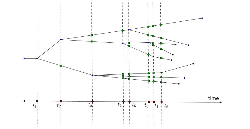
Figure 1: Construction of $\widetilde{T}$: The green nodes were introduced into the tree ‘by hand’.

• $\{(0,0,\dots)\}=\{u(0)\}={\tau}(0)$.

• for all $j\geq 0$, for all $t\in[t_{j},t_{j+1})$, ${\tau}(t)={\tau}(t_{j})$.

• If $u\in{\tau}(t_{j})$ then $u+(\underbrace{0,\dots,0}_{W(t_{j})\times 0},k,0,\dots)\in{\tau}(t_{j+1})$ if $0\leq k\leq l^{u}(t_{j+1})-1$, where

  $$l^{u}(t_{j})=\#\{\mbox{ offsprings of the particle corresponding to }u\,\mbox{at time}\,t_{j}\}.$$ (2.3)

Note that we use the convention that, if a given branch of the tree does not ”branch” at time $t_{j}$, we add to the underlying Galton-Watson at this time an extra vertex where $l^{u}(t_{j})=1$. (see Figure 1. The new vertices are the thick dots). We call the resulting tree $\widetilde{T}_{t}$.

We can relate the assignment of labels in a backwards consistent fashion as follows. For $u\equiv(u_{1},u_{2},u_{3},\dots)\in{\mathbb{Z}}_{+}^{\mathbb{N}}$, we define the function $u(r),r\in{\mathbb{R}}_{+}$, through

$$u_{\ell}(r)\equiv\begin{cases}u_{\ell},&\,\,\hbox{\rm if}\,\,t_{\ell}\leq r,\\ 0,&\,\,\hbox{\rm if}\,\,t_{\ell}>r.\end{cases}$$ (2.4)

Clearly, if $u(t)\in{\tau}(t)$ and $r\leq t$, then $u(r)\in{\tau}(r)$. This allows to define the boundary of the tree at infinity as follows:

$${\partial}\mathbf{T}\equiv\left\{u\in\mathbf{I}:\forall t<\infty,u(t)\in{\tau}(t)\right\}.$$ (2.5)

Note that ${\partial}\mathbf{T}$ is an ultrametric space equipped with the ultrametric $m(u,v)\equiv\mathrm{e}^{-d(u,v)}$, where $d(u,v)=\sup\{t\geq 0:u(t)=v(t)\}$ is the time of their most recent common ancestor.

In this way each leave of the Galton-Watson tree at time $t$, $i_{k}(t)$ with $k\in\{1,\dots,n(t)\}$ is identified with some multi-label $u^{k}(t)\in{\tau}(t)$. Then define

$$\gamma(u(t))\equiv\sum_{j=1}^{W(t)}{u_{j}(t)}\mathrm{e}^{-t_{j}}.$$ (2.6)

For a given $u$, the function $({\gamma}(u(t)),t\in{\mathbb{R}}_{+})$ describes a trajectory of a particle in ${\mathbb{R}}_{+}$. The important point is that, for a fixed particle, this trajectory converges to some point ${\gamma}(u)\in{\mathbb{R}}_{+}$, as $t\uparrow\infty$, almost surely. Hence also the sets ${\gamma}({\tau}(t))$ converge, for any realisation of the tree, to some (random) set ${\gamma}({\tau}(\infty))$.

Remark.

The labelling of the GW-tree is a slight variant of the familiar Ulam-Neveu-Harris labelling (see e.g. [18]). In our labelling the added zeros keep track of the order in which branching occurred in continuous time. We believe that this or an equivalent construction must be standard, but we have not been able to find it for continuous time trees in the literature.

In addition, in branching Brownian motion, there is also the position of the Brownian motion $x_{k}(t)$ of the $k$-th particle at time $t$. Hoping that there will not be too much confusion, we will often write ${\gamma}(x_{k}(t))\equiv{\gamma}(u^{k}(t))$. Thus to any ”particle” at time $t$ we can now associate the position on ${\mathbb{R}}\times{\mathbb{R}}_{+}$, $(x_{k}(t),{\gamma}(u^{k}(t)))$.

3 The extended convergence result

In this section we state the analog to (1.5) for branching Brownian motion. First let us recall the limit of the extremal process. Bramson [13] and Lalley and Sellke [21] show that, with $m(t)=\sqrt{2}t-\frac{3}{2\sqrt{2}}\ln t$,

$$\lim_{t\uparrow\infty}{\mathbb{P}}\left(\max_{k\leq n(t)}x_{k}(t)-m(t)\leq x\right)=\omega(x)={\mathbb{E}}\left[\mathrm{e}^{-CZ\mathrm{e}^{-\sqrt{2}x}}\right],$$ (3.1)

for some constant $C$, and where $Z\equiv\lim_{t\uparrow\infty}Z_{t}$ is the limit of the derivative martingale

$$Z_{t}\equiv\sum_{j\leq n(t)}(\sqrt{2}t-x_{j}(t))\mathrm{e}^{\sqrt{2}(x_{j}(t)-\sqrt{2}t)}.$$ (3.2)

In [4] and [1] it was shown that the process,

$${\mathcal{E}}_{t}\equiv\sum_{k=1}^{n(t)}{\delta}_{x_{k}(t)-m(t)}$$ (3.3)

converges, as $t\uparrow\infty$, in law to the process

$${\mathcal{E}}=\sum_{k,j}{\delta}_{\eta_{k}+{\Delta}^{(k)}_{j}},$$ (3.4)

where $\eta_{k}$ is the $k$-th atom of a Cox process with random intensity measure $CZ\mathrm{e}^{-\sqrt{2}y}dy$. The ${\Delta}^{(k)}_{i}$ are the atoms of independent and identically distributed point processes ${\Delta}^{(k)}$, which are copies of the limiting process

$${\Delta}\stackrel{{\scriptstyle D}}{{=}}\lim_{t\uparrow\infty}\sum_{i=1}^{n(t)}{\delta}_{\tilde{x}_{i}(t)-\max_{j\leq n(t)}\tilde{x}_{j}(t)},$$ (3.5)

where $\tilde{x}(t)$ is a BBM conditioned on $\max_{j\leq n(t)}\tilde{x}_{j}(t)\geq\sqrt{2}t$.

Using the embedding ${\gamma}$ defined in the previous section, we now state the following theorem, that exhibits more precisely the nature of the Poisson points and the genealogical structure of the extremal particles.

Theorem 3.1.

The point process $\widetilde{\mathcal{E}}_{t}\equiv\sum_{k=1}^{n(t)}{\delta}_{({\gamma}(u^{k}(t)),x_{k}(t)-m(t))}\rightarrow\widetilde{\mathcal{E}}$ on ${\mathbb{R}}_{+}\times{\mathbb{R}}$, as $t\uparrow\infty$, where

$$\widetilde{\mathcal{E}}\equiv\sum_{i,j}{\delta}_{(q_{i},p_{i})+(0,{\Delta}^{(i)}_{j})},$$ (3.6)

where $(q_{i},p_{i})_{i\in{\mathbb{N}}}$ are the atoms of a Cox process on ${\mathbb{R}}_{+}\times{\mathbb{R}}$ with intensity measure $Z(dv)\times C\mathrm{e}^{-\sqrt{2}x}dx$, where $Z(dv)$ is a random measure on ${\mathbb{R}}_{+}$, characterised in Proposition 3.2, and ${\Delta}_{j}^{(i)}$ are the atoms of independent and identically distributed point processes ${\Delta}^{(i)}$ as in (3.4) .

Remark.

The nice feature of the process $\widetilde{\mathcal{E}}_{t}$ is that it allows to visualise the different clusters ${\Delta}^{(i)}$ corresponding to the different point of the Poisson process of cluster extremes. In the process $\sum_{k=1}^{n(t)}{\delta}_{x_{k}(t)-m(t)}$ considered in earlier work, all these points get superimposed and cannot be disentangled. In other words, the process $\widetilde{\mathcal{E}}$ encodes both the values and the (rough) genealogical structure of the extremes of BBM.

The measure $Z(dv)$ in an interesting object in itself. For $v,r\in{\mathbb{R}}_{+}$ and $t>r$, we define

$$Z(v,r,t)=\sum_{j\leq n(t)}(\sqrt{2}t-x_{j}(t))\mathrm{e}^{\sqrt{2}(x_{j}(t)-\sqrt{2}t)}\mathbbm{1}_{{\gamma}(x_{j}(r))\leq v},$$ (3.7)

which is a truncated version of the usual derivative martingale $Z_{t}$. In particular, observe that $Z(\infty,r,t)=Z_{t}$.

Proposition 3.2.

For each $v\in{\mathbb{R}}_{+}$ the limit $\lim_{r\uparrow\infty}\lim_{t\uparrow\infty}Z(v,r,t)$ exists almost surely. Set

$$Z(v)\equiv\lim_{r\uparrow\infty}\lim_{t\uparrow\infty}Z(v,r,t).$$ (3.8)

Then $0\leq Z(v)\leq Z$, where $Z$ is the limit of the derivative martingale. Moreover, $Z(v)$ is monotone increasing in $v$ and the corresponding measure $Z(dv)$ is a.s. non-atomic.

The measure $Z(v)$ is the analogue of the corresponding ”derivative martingale measure” studied in Duplantier et al [15, 16] and Biskup and Louidor [9, 8] in the context of the Gaussian free field and in [7, 6] for the critical Mandelbrot multiplicative cascade. For a review, see Rhodes and Vargas [24]. The objects are examples of what is known as multiplicative chaos that was introduced by Kahane [19].

4 Properties of the embedding

We need the three basic properties of ${\gamma}$. Lemma 4.1 states that the map ${\gamma}(x_{k}(t))$ converges for all extremal particles, as $t\uparrow\infty$, and is well approximated by the information on the tree up to a fixed time $r$.

Lemma 4.1.

Let $D\subset{\mathbb{R}}$ be a compact set. Define, for $0\leq r<t<\infty$, the events

$$\mathcal{A}_{r,t}^{{\gamma}}(D)=\left\{\forall k\mbox{ with }x_{k}(t)-m(t)\in D\mbox{ : }{\gamma}(x_{k}(t))-{\gamma}(x_{k}(r))\leq\mathrm{e}^{-r/2}\right\}.$$ (4.1)

For any $\epsilon>0$ there exists $0\leq r(D,\epsilon)<\infty$ such that, for any $r>r(D,\epsilon)$ and $t>3r$

$${\mathbb{P}}\left(\left(\mathcal{A}_{r,t}^{{\gamma}}(D)\right)^{c}\right)<\epsilon.$$ (4.2)

Proof.

Set $\overline{D}\equiv\sup\{x\in D\}$ and $\underline{D}\equiv\inf\{x\in D\}$. Let $\epsilon>0$. Then, by Theorem 2.3 of [2], for each $\epsilon>0$ there exists $r_{1}<\infty$ such that, for all $t>3r_{1}$,

$${\mathbb{P}}\left(\left(\mathcal{A}_{r,t}^{{\gamma}}(D)\right)^{c}\right) \leq {\mathbb{P}}\big{(}\exists k:x_{k}(t)-m(t)\in D,\forall_{s\in[r_{1},t-r_{1}]}:x_{k}(s)\leq\overline{D}+E_{t,{\alpha}}(s)$$ (4.3)

$$\qquad\mbox{ but }{\gamma}(x_{k}(t))-{\gamma}(x_{k}(r))>\mathrm{e}^{-r/2}\big{)}+\epsilon/2,$$

where $0<{\alpha}<\frac{1}{2}$ and $E_{t,{\alpha}}(s)=\frac{s}{t}m(t)-f_{t,{\alpha}}(s)$ and $f_{t,{\alpha}}=(s\wedge(t-s))^{{\alpha}}$. Using the ”many-to-one lemma” (see Theorem 8.5 of [17])), the probability in (4.3) is bounded from above by

$$\mathrm{e}^{t}{\mathbb{P}}\left(x(t)\in m(t)+D,\forall_{s\in[r_{1},t-r_{1}]}:x(s)\leq\overline{D}+E_{t,{\alpha}}(s)\mbox{ but }\textstyle\sum_{j}m_{j}\mathrm{e}^{-\tilde{t}_{j}}\mathbbm{1}_{\tilde{t}_{j}\in[r,t]}>\mathrm{e}^{-r/2}\right),$$ (4.4)

where $x$ is a standard Brownian motion and $(\tilde{t}_{j},j\in{\mathbb{N}})$ are the points of a size-biased Poisson point process with intensity measure $2dx$ independent of $x$, $m_{j}$ are independent random variables uniformly distributed on $\{0,\dots,\tilde{l}_{j}-1\}$, where finally $\tilde{l}_{j}$ are i.i.d. according to the size-biased offspring distribution, ${\mathbb{P}}(\tilde{l}_{j}=k)=\frac{kp_{k}}{2}$. Due to independence, and since $m_{j}\leq\tilde{l}_{j}$, the expression (4.4) is bounded from above by

$$\mathrm{e}^{t}{\mathbb{P}}\left(x(t)\in m(t)+D,\forall_{s\in[r_{1},t-r_{1}]}:x(s)\leq\overline{D}+E_{t,{\alpha}}(s)\right)$$

$$\quad\times{\mathbb{P}}\left(\textstyle\sum_{j}(\tilde{l}_{j}-1)\mathrm{e}^{-\tilde{t}_{j}}\mathbbm{1}_{\tilde{t}_{j}\in[r,t]}>\mathrm{e}^{-r/2}\right).$$ (4.5)

The first probability in (4) is bounded by

$${\mathbb{P}}\left(x(t)\in m(t)+D,\forall_{s\in[r_{1},t-r_{1}]}:x(s)-\frac{s}{t}x(t)\leq\overline{D}-\underline{D}-f_{t,{\alpha}}(s)\right).$$ (4.6)

Using that $\xi(s)\equiv x(s)-\frac{s}{t}x(t)$ is a Brownian bridge from $0$ to $0$ in time $t$ that is independent of $x(t)$, (4.6) equals

$${\mathbb{P}}\left(x(t)\in m(t)+D\right){\mathbb{P}}\left(\forall_{s\in[r_{1},t-r_{1}]}:\xi(s)\leq\overline{D}-\underline{D}-f_{t,{\alpha}}(s)\right)$$

$$\leq{\mathbb{P}}\left(x(t)\in m(t)+D\right){\mathbb{P}}\left(\forall_{s\in[r_{1},t-r_{1}]}:\xi(s)\leq\overline{D}-\underline{D}\right).$$ (4.7)

Using now Lemma 3.4 of [2] to bound the last factor of (4) we obtain that (4) is bounded from above by

$${\kappa}\frac{r_{1}}{t-2r_{1}}{\mathbb{P}}\left(x(t)\in m(t)+D\right),$$ (4.8)

where ${\kappa}<\infty$ is a positive constant. Using this as an upper bound for the first probability in (4) we can bound (4) from above by

$$\mathrm{e}^{t}{\kappa}\frac{r_{1}}{t-2r_{1}}{\mathbb{P}}\left(x(t)\in m(t)+D\right){\mathbb{P}}\left(\textstyle\sum_{j}(\tilde{l}_{j}-1)\mathrm{e}^{-\tilde{t}_{j}}\mathbbm{1}_{\tilde{t}_{j}\in[r,t]}>\mathrm{e}^{-r/2}\right).$$ (4.9)

By (5.25) of [2](or an easy Gaussian computation) this is bounded from above by

$$C{\kappa}\frac{r_{1}t}{t-2r_{1}}{\mathbb{P}}\left(\textstyle\sum_{j}(\tilde{l}_{j}-1)\mathrm{e}^{-\tilde{t}_{j}}\mathbbm{1}_{\tilde{t}_{j}\in[r,t]}>\mathrm{e}^{-r/2}\right),$$ (4.10)

for some positive constant $C<\infty$. Using the Markov inequality, (4.10) is bounded from above by

$$C{\kappa}\frac{tr_{1}}{t-2r_{1}}\mathrm{e}^{r/2}{\mathbb{E}}\left(\textstyle\sum_{j}(\tilde{l}_{j}-1)\mathrm{e}^{-\tilde{t}_{j}}\mathbbm{1}_{\tilde{t}_{j}\in[r,t]}\right),$$ (4.11)

We condition on the ${\sigma}$-algebra $\mathcal{F}$ generated by the Poisson points. Using that $\tilde{l}_{j}$ is independent of the Poisson point process $(\tilde{t}_{j})_{j}$ and $\sum_{j}\mathrm{e}^{-\tilde{t}_{j}}\mathbbm{1}_{\tilde{t}_{j}\in[r,t]}$ is measurable with respect to $\mathcal{F}$ we obtain that (4.11) is equal to

$$C{\kappa}\frac{tr_{1}}{t-2r_{1}}\mathrm{e}^{r/2}{\mathbb{E}}\left({\mathbb{E}}\left(\textstyle\sum_{j}(\tilde{l}_{j}-1)\mathrm{e}^{-\tilde{t}_{j}}\mathbbm{1}_{\tilde{t}_{j}\in[r,t]}|\mathcal{F}\right)\right)$$ (4.12)

$$=C{\kappa}\frac{tr_{1}}{t-2r_{1}}\mathrm{e}^{r/2}{\mathbb{E}}\left(\textstyle\sum_{j}\mathrm{e}^{-\tilde{t}_{j}}\mathbbm{1}_{\tilde{t}_{j}\in[r,t]}{\mathbb{E}}\left((\tilde{l}_{j}-1)|\mathcal{F}\right)\right).$$

Since ${\mathbb{E}}(l_{j}-1)=\sum_{k}\frac{1}{2}(k-1)kp_{k}=K/2<\infty$ we have that (4.12) is equal to

$$C{\kappa}K/2\frac{tr_{1}}{t-2r_{1}}\mathrm{e}^{r/2}{\mathbb{E}}\left(\textstyle\sum_{j}\mathrm{e}^{-\tilde{t}_{j}}\mathbbm{1}_{\tilde{t}_{j}\in[r,t]}\right).$$ (4.13)

By Campbell’s theorem (see e.g [20] ), (4.13) is equal to

$$C{\kappa}K/2\frac{tr_{1}}{t-2r_{1}}\mathrm{e}^{r/2}\int_{r}^{t}\mathrm{e}^{-x}2dx\leq C{\kappa}K\frac{tr_{1}}{t-2r_{1}}\mathrm{e}^{-r/2},$$ (4.14)

which is smaller than $\epsilon/2$, for all $r$ sufficiently large and $t>3r$.

∎

The second lemma now ensures that ${\gamma}$ maps particles, that are extremal, with low probability to a very small neighbourhood of a fixed $a\in{\mathbb{R}}$.

Lemma 4.2.

Let $a\in{\mathbb{R}}_{+}$ and $D\subset{\mathbb{R}}$ be a compact set. Define the event

$$\mathcal{B}^{{\gamma}}_{r,t}(D,a,{\delta})=\left\{\forall k\mbox{ with }x_{k}(t)-m(t)\in D\mbox{: }{\gamma}(x_{k}(r))\not\in[a-{\delta},a]\right\}.$$ (4.15)

For any $\epsilon>0$ there exists ${\delta}>0$ and $r(a,D,{\delta},\epsilon)$ such that, for any $r>r(a,D,{\delta},\epsilon)$ and $t>3r$

$${\mathbb{P}}\left(\left(\mathcal{B}^{{\gamma}}_{r,t}(D,a,{\delta})\right)^{c}\right)<\epsilon.$$ (4.16)

Proof.

Following the proof of Lemma 4.1 step by step we arrive at the bound

$${\mathbb{P}}\left(\left(\mathcal{B}^{{\gamma}}_{r,t}(D,a,{\delta})\right)^{c}\right)\leq C{\kappa}\frac{tr_{1}}{t-2r_{1}}{\mathbb{P}}\left(\textstyle\sum_{j}m_{j}\mathrm{e}^{-\tilde{t}_{j}}\mathbbm{1}_{\tilde{t}_{j}\in[0,r]}\in[a-{\delta},a]\right).$$ (4.17)

We rewrite the probability in (4.17) in the form

$$\sum_{i^{*}=1}^{\infty}{\mathbb{P}}\left(i^{*}=\inf\{i:m_{i}\neq 0\},\textstyle\sum_{j\geq i^{*}}m_{j}\mathrm{e}^{-\tilde{t}_{j}}\mathbbm{1}_{\tilde{t}_{j}\in[0,r]}\in[a-{\delta},a]\right).$$ (4.18)

Consider first ${\mathbb{P}}\left(i^{*}=\inf\{i:m_{i}\neq 0\}\right)$. This probability is equal to

$${\mathbb{P}}\left(\forall_{i\leq i^{*}}:m_{i}=0\mbox{ and }m_{i^{*}}\neq 0\right)={\mathbb{E}}\left[\left(1-\frac{1}{l_{i^{*}}}\right)\prod_{j=1}^{i^{*}-1}\frac{1}{l_{j}}\right].$$ (4.19)

Using that the $l_{j}$ are iid together with the simple bound ${\mathbb{E}}\left(l_{j}^{-1}\right)\leq\frac{1+p_{1}}{2}$, we see that (4.19) is bounded from above by

$$\left(\frac{1+p_{1}}{2}\right)^{i^{*}-1}.$$ (4.20)

Since $\frac{1+p_{1}}{2}<1$ by assumption on $p_{1}$ we can choose, for each $\epsilon^{\prime}>0$ $K(\epsilon^{\prime})<\infty$ such that

$$\sum_{i^{*}=K(\epsilon^{\prime})+1}^{\infty}\left(\frac{1+p_{1}}{2}\right)^{i^{*}-1}<\epsilon^{\prime}.$$ (4.21)

Hence we bound (4.18) by

$$\sum_{i^{*}=1}^{K(\epsilon^{\prime})}{\mathbb{P}}\left(i^{*}=\inf\{i:m_{i}\neq 0\},\textstyle\sum_{j\geq i^{*}}m_{j}\mathrm{e}^{-\tilde{t}_{j}}\mathbbm{1}_{\tilde{t}_{j}\in[0,r]}\in[a-{\delta},a]\right)+\epsilon^{\prime}.$$ (4.22)

We rewrite

$$\textstyle\sum_{j\geq i^{*}}m_{j}\mathrm{e}^{-\tilde{t}_{j}}\mathbbm{1}_{\tilde{t}_{j}\in[0,r]}=m_{i^{*}}\mathrm{e}^{-\tilde{t}_{i^{*}}}\mathbbm{1}_{\tilde{t}_{i^{*}}\in[0,r]}\left(1+m_{i^{*}}^{-1}\sum_{j>i^{*}}m_{j}\mathrm{e}^{-(\tilde{t}_{j}-\tilde{t}_{i^{*}})}\mathbbm{1}_{\tilde{t}_{j}-t_{i}^{*}\in[0,r-t_{i^{*}}]}\right)$$ (4.23)

Next, we estimate the probability that $\tilde{t}_{i^{*}}$ is large. Observe that $\tilde{t}_{i^{*}}=\sum_{i=1}^{i^{*}}s_{i}$ where $s_{i}$ are iid exponentially distributed random variables with parameter $2$. This implies that $\tilde{t}_{i^{*}}$ is Erlang$(2,i^{*})$. Thus

$${\mathbb{P}}\left(\tilde{t}_{i^{*}}>r^{\alpha}\right)=\mathrm{e}^{-2r^{\alpha}}\textstyle\sum_{i=0}^{i^{*}}\frac{(2r^{{\alpha}})^{i}}{i!}\leq\mathrm{e}(2r^{\alpha})^{K(\epsilon^{\prime})}\mathrm{e}^{-2r^{\alpha}},\mbox{ for all }i^{*}\leq K(\epsilon^{\prime}).$$ (4.24)

Next we want to replace $\tilde{t}_{i^{*}}$ in the indicator function in (4.23) by a non-random quantity $r^{\alpha}$, for some $0<{\alpha}<1$, in order to have a bound that depends only on the differences $\tilde{t}_{j}-\tilde{t}_{i^{*}}$. Note first that

$$\sum_{j>i^{*}}m_{j}\mathrm{e}^{-(\tilde{t}_{j}-\tilde{t}_{i^{*}})}\mathbbm{1}_{\tilde{t}_{j}-t_{i}^{*}\in[0,r-t_{i^{*}}]}-\sum_{j>i^{*}}m_{j}\mathrm{e}^{-(\tilde{t}_{j}-\tilde{t}_{i^{*}})}\mathbbm{1}_{\tilde{t}_{j}-t_{i}^{*}\in[0,r-r^{\alpha}]}$$ (4.25)

$$=\sum_{j>i^{*}}m_{j}\mathrm{e}^{-(\tilde{t}_{j}-\tilde{t}_{i^{*}})}\mathbbm{1}_{\tilde{t}_{j}-t_{i}^{*}\in[r-r^{\alpha},r-t_{i^{*}}]}\leq\sum_{j>i^{*}}m_{j}\mathrm{e}^{-(\tilde{t}_{j}-\tilde{t}_{i^{*}})}\mathbbm{1}_{\tilde{t}_{j}-t_{i}^{*}\in[r-r^{\alpha},r]}.$$

Using the fact that $m_{j}\leq\tilde{l}_{j}-1$, for all $j$ and the Markov inequality, we get that

$${\mathbb{P}}\left(\textstyle\sum_{j>i^{*}}m_{j}\mathrm{e}^{-(\tilde{t}_{j}-\tilde{t}_{i^{*}})}\mathbbm{1}_{\tilde{t}_{j}-\tilde{t}_{i^{*}}\in[r-r^{\alpha},r]}>\mathrm{e}^{-r/2}\right)$$

$$\leq\mathrm{e}^{r/2}{\mathbb{E}}\left(\textstyle\sum_{j>i^{*}}(\tilde{l}_{j}-1)\mathrm{e}^{-(\tilde{t}_{j}-\tilde{t}_{i^{*}})}\mathbbm{1}_{\tilde{t}_{j}-\tilde{t}_{i^{*}}\in[r-r^{\alpha},r]}\right).$$ (4.26)

Using Campbell’s theorem as in (4.12), we see that the second line in (4) is equal to

$$\mathrm{e}^{r/2}K/2\int_{r-r^{\alpha}}^{r}\mathrm{e}^{-x}2dx=K\left(\mathrm{e}^{-r/2+r^{\alpha}}-\mathrm{e}^{-r/2}\right).$$ (4.27)

For any $\epsilon^{\prime}>0$, there exists $r_{0}<\infty$, such that, for all $r>r_{0}$, the probabilities in (4.24) and (4) are smaller than $\epsilon^{\prime}$. On the the event

$$\mathcal{D}=\{t_{i^{*}}\leq r^{\alpha}\}\cap\left\{\sum_{j>i^{*}}m_{j}\mathrm{e}^{-(\tilde{t}_{j}-\tilde{t}_{i^{*}})}\mathbbm{1}_{\tilde{t}_{j}-t_{i}^{*}\in[r-r^{\alpha},r]}\leq\mathrm{e}^{-r/2}\right\},$$ (4.28)

which has probability at least $1-2\epsilon^{\prime}$, we can bound (4.22) in a nice way. Namely, since $m_{i^{*}}\geq 1$ by definition and $m_{j}$ are chosen uniformly from $(0,\dots,l_{j}-1)$ and independent of $\{t_{j}\}_{j\geq 1}$. Moreover, $\sum_{j>i^{*}}m_{j}\mathrm{e}^{-(\tilde{t}_{j}-\tilde{t}_{i^{*}})}\mathbbm{1}_{\tilde{t}_{j}-t_{i^{*}}\in[0,r-r^{\alpha}]}\geq 0$ is also independent of $t_{i*}$. It follows that (4.22) is bounded from above by

$$\sum_{i^{*}=1}^{K(\epsilon^{\prime})}{\mathbb{P}}\left(i^{*}=\inf\{i:m_{i}\neq 0\}\right)\max_{b\in[0,1]}{\mathbb{P}}\left(\{\mathrm{e}^{-\tilde{t}_{i^{*}}}\in[b-{\delta}-\mathrm{e}^{-r/2},b]\}\land\{t_{i^{*}}\leq r^{\alpha}\}\right)+3\epsilon^{\prime}.$$ (4.29)

Using the bound on the first probability in (4.29) given in (4.20), one sees that (4.29) is bounded from above by

$$\sum_{i^{*}=1}^{K(\epsilon^{\prime})}\left(\frac{1+p_{1}}{2}\right)^{i^{*}-1}\max_{b\in[{\delta}+\mathrm{e}^{-r^{\alpha}}+\mathrm{e}^{-r/2},1]}{\mathbb{P}}\left(t_{i^{*}}\in\left[-\log b,-\log\left(b-{\delta}-\mathrm{e}^{-r/2}\right)\right]\right)+3\epsilon^{\prime}$$ (4.30)

Recalling that $t_{i^{*}}$ is Erlang$(2,i^{*})$ distributed, we have that

$${\mathbb{P}}\left(t_{i^{*}}\in\left[-\log b,-\log\left(b-{\delta}-\mathrm{e}^{-r/2}\right)\right]\right)$$

$$=\sum_{i=0}^{i^{*}-1}\frac{1}{i!}\left(f_{i}(b-{\delta}-\mathrm{e}^{r/2})-f_{i}(b)\right),$$ (4.31)

where we have set $f_{i}(x)=x^{2}\left(-2\log(x)\right)^{i}$. By the mean value theorem, uniformly on $b\in[{\delta}+\mathrm{e}^{-r^{\alpha}}+\mathrm{e}^{-r/2},1]$,

$$0\leq f_{i}(b)-f_{i}(b-{\delta}-\mathrm{e}^{-r/2})\leq 2(2{r^{\alpha}}))^{i}(i+2r^{\alpha})\left({\delta}+\mathrm{e}^{-r/2}\right).$$ (4.32)

Inserting this bound into (4), we get that, for $i^{*}\leq K(\epsilon^{\prime})$,

$$\max_{b\in[{\delta}+\mathrm{e}^{-r^{\alpha}}+\mathrm{e}^{-r/2},1]}{\mathbb{P}}\left(t_{i^{*}}\in\left[-\log b,-\log\left(b-{\delta}-\mathrm{e}^{-r/2}\right)\right]\right)$$ (4.33)

$$\leq 4({\delta}+\mathrm{e}^{-r/2})\sum_{i=0}^{i^{*}}\frac{1}{i!}(2r^{\alpha})^{i}\leq 4\mathrm{e}({\delta}+\mathrm{e}^{-r/2})\mathrm{e}^{2r^{\alpha}}.$$

Now we choose $r$ so big that $4\mathrm{e}^{-r/2+2r^{\alpha}+1}\leq\epsilon^{\prime}/2$ and then ${\delta}$ so small that ${\delta}4\mathrm{e}^{2r^{\alpha}+1}\leq\epsilon^{\prime}/2$, so that the entire expression on the right is bounded by $\epsilon^{\prime}$. Collecting the bounds in (4.24), (4) and (4) implies (4.16) if $\epsilon^{\prime}=\epsilon/4$ ∎

The following lemma asserts that any two points that get close to the maximum of BBM, have distinct images under the map ${\gamma}$, unless the time of the most recent common ancestor is large. This implies in particular that the positions of the cluster extremes all differ in the second coordinate. This lemma is not strictly needed in the proof of our main theorem, but we find it nice to make this point explicit. The proof uses largely the same arguments that were used in the proofs of Lemmas 4.1 and 4.2.

Lemma 4.3.

Let $D\subset{\mathbb{R}}$ be a compact set. For any $\epsilon>0$ there exists $\delta>0$ and $r({\delta},\epsilon)$ such that, for any $r>r({\delta},\epsilon)$ and $t>3r$

$${\mathbb{P}}\left(\exists_{i,j\leq n(t):d(x_{i}(t),x_{j}(t))\leq r}:x_{i}(t),x_{j}(t)\in m(t)+D,|{\gamma}(x_{i}(t))-{\gamma}(x_{j}(t))|\leq{\delta}\right)<\epsilon.$$ (4.34)

Proof.

To control (4.34), we first use that, by Theorem 2.1 in [2], for any $\epsilon^{\prime}$, there is $r_{1}<\infty$, such that, for all $t\geq 3r_{1}$, and $r\leq t/3$, the event

$$\{\exists_{i,j\leq n(t):d(x_{i}(t),x_{j}(t))\in(r_{1},r)},x_{i}(t),x_{j}(t)\in m(t)+D\}$$ (4.35)

has probability smaller than $\epsilon^{\prime}$. Therefore,

$${\mathbb{P}}\left(\exists_{i,j\leq n(t):d(x_{i}(t),x_{j}(t))\leq r}:x_{i}(t),x_{j}(t)\in m(t)+D,|{\gamma}(x_{i}(t))-{\gamma}(x_{j}(t))|\leq{\delta}\right)$$ (4.36)

$$\leq{\mathbb{P}}\left(\exists_{i,j\leq n(t):d(x_{i}(t),x_{j}(t))\leq r_{1}}:x_{i}(t),x_{j}(t)\in m(t)+D,|{\gamma}(x_{i}(t))-{\gamma}(x_{j}(t))|\leq{\delta}\right)+\epsilon^{\prime}.$$

The nice feature of the probability in the last line is that $r_{1}$ is now independent of $r$.

To bound the probability in the last line, we proceed as follows: at time $r_{1}$, there are $n(r_{1})$ particles alive. From these we select the ancestors of the particles $i$ and $j$. This gives at most $n(r_{1})^{2}$ choices. The offspring of these particle are then independent, conditional on what happened up to time $r_{1}$, i.e. the ${\sigma}$-algebra ${\mathcal{F}}_{r_{1}}$. We denote the offspring of these two particles starting from time $r_{1}$ by $\tilde{x}^{(1)}$ and $\tilde{x}^{(2)}$. In this way, we write this probability in the form

$${\mathbb{E}}\left[\sum_{\ell\neq\ell^{\prime}=1}^{n(r_{1})}{\mathbb{P}}\left(\dots\big{|}{\mathcal{F}}_{r_{1}}\right)\right],$$ (4.37)

where

$${\mathbb{P}}\left(\dots\big{|}{\mathcal{F}}_{r_{1}}\right)$$

$$={\mathbb{P}}\Bigl{(}\exists_{i\leq n^{(1)}(t-r_{1}),j\leq n^{(2)}(t-r_{1})}:x_{\ell}(r_{1})+\tilde{x}^{(1)}_{i}(t-r_{1}),x_{\ell^{\prime}}(r_{1})+x^{(2)}_{j}(t-r_{1})\in m(t)+D,$$

$$\quad|{\gamma}(x_{\ell}(r_{1})+x^{(1)}_{i}(t-r_{1}))-{\gamma}(x_{\ell^{\prime}}(r_{1})+x^{(2)}_{j}(t-r_{1}))|\leq{\delta}\Big{|}{\mathcal{F}}_{r_{1}}\Bigr{)}.$$ (4.38)

The conditional probability is a function of $x_{\ell}(r_{1})$ and $x_{\ell^{\prime}}(r_{1})$ only, and we will bound it uniformly on a set of large probability. Note first that we can chose as finite enlargement, $\widetilde{D}$, of the set $D$ (depending only on the value of $r_{1}$), such that such that $D+x_{k}(r_{1})\subset\widetilde{D}$ and $D+x_{\ell}(r_{1})\in\widetilde{D}$ with probability at least $1-\epsilon^{\prime\prime}$. For such $x_{\ell}(r_{1}),x_{\ell^{\prime}}(r_{2})$, (4) is bounded from above by

$${\mathbb{P}}\Bigl{(}\exists_{i\leq n^{(1)}(t-r_{1}),j\leq n^{(2)}(t-r_{1})}:\tilde{x}^{(1)}_{i}(t-r_{1}),\tilde{x}^{(2)}_{j}(t-r_{1})\in m(t)+\widetilde{D},$$

$$\quad|{\gamma}(x_{\ell}(r_{1})+\tilde{x}^{(1)}_{i}(t-r_{1}))-{\gamma}(x_{\ell^{\prime}}(r_{1})+\tilde{x}^{(2)}_{j}(t-r_{1}))|\leq{\delta}\Big{|}{\mathcal{F}}_{r_{1}}\Bigr{)}.$$ (4.39)

Next, we notice that, at the expense of a further error $\epsilon^{\prime\prime}$, we can introduce the condition that the paths stay below the curves $E_{t-r_{1},{\alpha}}(s)$, for all $(r_{2},t-r_{1}-r_{2})$, for some $r_{2}$ depending only on $\epsilon^{\prime\prime}$. Using the independence of the BBMs $\tilde{x}^{(1)}$ and $\tilde{x}^{(2)}$, and proceeding otherwise as in (4), we can bound (4) from above by

$$\epsilon^{\prime\prime}+\left(C{\kappa}\frac{(t-r_{1})r_{2}}{t-r_{1}-2r_{2}}\right)^{2}$$ (4.40)

$$\times\;{\mathbb{P}}\left(\Big{|}{\gamma}(x_{\ell}(r_{1}))-{\gamma}(x_{\ell^{\prime}}(r_{1}))+\textstyle\sum_{k}m_{k}^{j}\mathrm{e}^{-\tilde{t}_{k}^{j}}\mathbbm{1}_{\tilde{t}_{k}^{j}\in[r_{1},t]}-\textstyle\sum_{k^{\prime}}m_{k^{\prime}}^{i}\mathrm{e}^{-\tilde{t}_{k^{\prime}}^{i}}\mathbbm{1}_{\tilde{t}_{k^{\prime}}^{i}\in[r_{1},t]}\Big{|}\leq{\delta}\Big{|}{\mathcal{F}}_{r_{1}}\right),$$

where $(\tilde{t}_{k}^{j},k\in{\mathbb{N}})$ and $(\tilde{t}_{k^{\prime}}^{i},k^{\prime}\in{\mathbb{N}})$ are the points of independent Poisson point processes with intensity $2dx$ restricted to $[r_{1},t]$. Moreover, $l_{k}^{j},l_{k^{\prime}}^{i}$ are i.i.d. according to the size-biased offspring distribution and $m_{k}^{j}$ resp. $m_{k^{\prime}}^{i}$ are uniformly distributed on $\{0,\dots,l_{k}^{j}-1\}$ resp. $\{0,\dots,l_{k^{\prime}}^{i}-1\}$. We rewrite (4.40) as

$${\mathbb{P}}\left(\textstyle\sum_{k}m_{k}^{j}\mathrm{e}^{-\tilde{t}_{k}^{j}}\mathbbm{1}_{\tilde{t}_{k}^{j}\in[r_{1},t]}\in{\gamma}(x_{\ell^{\prime}}(r_{1}))-{\gamma}(x_{\ell}(r_{1}))+\textstyle\sum_{k^{\prime}}m_{k^{\prime}}^{i}\mathrm{e}^{-\tilde{t}_{k^{\prime}}^{i}}\mathbbm{1}_{\tilde{t}_{k^{\prime}}^{j}\in[r_{1},t]}+[-{\delta},{\delta}]\Big{|}{\mathcal{F}}_{r_{1}}\right).$$ (4.41)

As in (4.18) we rewrite the probability in (4.41) as

$$\sum_{l=1}^{\infty}{\mathbb{P}}\Bigl{(}l=\inf\{k:m_{k}^{j}\neq 0\},\;$$ (4.42)

$$\textstyle\sum_{k\geq l}m_{k}^{j}\mathrm{e}^{-\tilde{t}_{k}^{j}}\mathbbm{1}_{\tilde{t}_{k}^{j}\in[r_{1},t]}\in{\gamma}(x_{\ell^{\prime}}(r_{1}))-{\gamma}(x_{\ell}(r_{1}))+\textstyle\sum_{k^{\prime}}m_{k^{\prime}}^{i}\mathrm{e}^{-\tilde{t}_{k^{\prime}}^{i}}\mathbbm{1}_{\tilde{t}_{k^{\prime}}^{j}\in[r_{1},t]}+[-{\delta},{\delta}]\Big{|}{\mathcal{F}}_{r_{1}}\Bigr{)}.$$

Due to the independence of $(\tilde{t}_{k}^{j},k\in{\mathbb{N}})$ and $(\tilde{t}_{k^{\prime}}^{i},k^{\prime}\in{\mathbb{N}})$ we can proceed as with (4.18) in the proof of Lemma 4.2 to make (4.42) as small as desired, independently on the value of ${\gamma}(x_{\ell^{\prime}}(r_{1}))-{\gamma}(x_{\ell}(r_{1}))$ by choosing ${\delta}$ small enough. Collecting all terms, we see that (4.37) is bounded by

$${\mathbb{E}}\left[\sum_{\ell\neq\ell^{\prime}=1}^{n(r_{1})}{\mathbb{P}}\left(\dots\big{|}{\mathcal{F}}_{r_{1}}\right)\right]\leq 4\epsilon^{\prime\prime}{\mathbb{E}}\left[\sum_{\ell\neq\ell^{\prime}=1}^{n(r_{1})}1\right]\leq 4\epsilon^{\prime\prime}K\mathrm{e}^{2r_{1}}.$$ (4.43)

Choosing $\epsilon^{\prime\prime}$ and $\epsilon^{\prime}$ small enough, this yields the assertion of Lemma 4.3. ∎

5 The $q$-thinning

The proof of the convergence of $\sum_{i=1}^{n(t)}{\delta}_{({\gamma}(x_{i}(t)),x_{i}(t)-m(t))}$ comes in two main steps. In a first step, we show that the points of the local extrema converge to the desired Poisson point process. To make this precise, we work with the concept of thinning classes that was already introduced in [3]. We repeat the construction here for completeness and introduce the corresponding notation.

Assume here and in the sequel that the particles at time $t$ are labeled in decreasing order

$$x_{1}(t)\geq x_{2}(t)\geq\dots\geq x_{n(t)}(t),$$ (5.1)

and set $\bar{x}_{k}(t)\equiv x_{k}(t)-m(t)$. Let

$$\bar{Q}(t)=\{\bar{Q}_{i,j}(t)\}_{i,j\leq n(t)}\equiv\{t^{-1}Q_{i,j}(t)\}_{i,j\leq n(t)},$$ (5.2)

where

$$Q_{i,j}(t)=\sup\{s\leq t:x_{i}(s)=x_{j}(s)\}=d(u^{i}(t),u^{j}(t)).$$ (5.3)

$(\mathcal{E}(t),\bar{Q}(t))$ admits the following thinning. For any $q\geq 0$ the following is true: If $\bar{Q}_{i,j}(t)\geq q$ and $\bar{Q}_{j,k}(t)\geq q$, then $\bar{Q}_{i,k}(t)\geq q$. Therefore, the sets $\{i,j\in\{1,\dots,n(t)\}:\bar{Q}_{i,j}(t)\geq q\}$ form a partition of the set $\{1,\dots,n(t)\}$ into equivalence classes. We select the maximal particle of each equivalence class as representative in the following recursive manner:

$$i_{1}=1$$

$$i_{k}=\min\{j\geq i_{k-1}:\bar{Q}_{i,j}(t)<q,\;\forall i\leq k-1\},$$ (5.4)

if such an $j$ exists. If no such $j$ exists, we denote $k-1=n^{*}(t)$ and terminate the procedure. The $q$- thinning process of $(\mathcal{E}(t),\bar{Q}(t))$, denoted by $\mathcal{E}^{(q)}(t)$ is defined by

$$\mathcal{E}^{(q)}(t)=\sum_{k=1}^{n^{*}(t)}{\delta}_{\bar{x}_{i_{k}}(t)}.$$ (5.5)

6 Extended convergence of thinned point process

For $r_{d}\in{\mathbb{R}}_{+}$ and $t>3r_{d}$ consider the thinned process ${\mathcal{E}}^{(r_{d}/t)}(t)$. Observe that, for $R_{t}=m(t)-m(t-r_{d})-\sqrt{2}r_{d}=o(1)$, we have

$${\mathcal{E}}^{(r_{d}/t)}(t)\stackrel{{\scriptstyle D}}{{\equiv}}\sum_{j=1}^{n(r_{d})}{\delta}_{x_{j}(r_{d})-\sqrt{2}r_{d}+M_{j}(t-r_{d})-R_{t}}$$ (6.1)

where $M_{j}(t-r_{d})\equiv\max_{k\leq n^{(j)}(t-r_{d})}x_{k}^{(j)}(t-r_{d})-m(t-r_{d})$ and $x^{(j)}$ are independent BBM’s (see (3.15) in [3]). Then

Proposition 6.1.

Let $\mathcal{E}^{(r_{d}/t)}(t)$ and $n^{*}(t)$ be defined in (5.5) for $q=r_{d}/t$. Then

$$\lim_{r_{d}\uparrow\infty}\lim_{t\uparrow\infty}\sum_{k=1}^{n^{*}(t)}{\delta}_{({\gamma}(x_{i_{k}}(t)),\bar{x}_{i_{k}}(t))}\stackrel{{\scriptstyle D}}{{=}}\sum_{i}{\delta}_{(q_{i},p_{i})}\equiv\widehat{\mathcal{E}},$$ (6.2)

where $(q_{i},p_{i})_{i\in{\mathbb{N}}}$ are the points of the Cox process $\widehat{\mathcal{E}}$ with intensity measure $Z(dv)\times C\mathrm{e}^{-\sqrt{2}x}dx$ with the random measure $Z(dv)$ defined in (3.8). Moreover,

$$\lim_{r\uparrow\infty}\lim_{r_{d}\uparrow\infty}\sum_{j=1}^{n(r_{d})}{\delta}_{(\gamma(x_{j}(r)),x_{j}(r_{d})-\sqrt{2}r_{d}+M_{j})}\stackrel{{\scriptstyle D}}{{=}}\widehat{\mathcal{E}},$$ (6.3)

where $M_{j}$ are i.i.d with law $\omega$ defined in (3.1).

The proof of Proposition 6.1 relies on Proposition 3.2 which we now prove.

Proof of Proposition 3.2.

For $v,r\in{\mathbb{R}}_{+}$ fixed, the process $Z(v,r,t)$ defined in (3.7) is a martingale in $t>r$ (since $Z(\infty,r,t)$ is the derivative martingale and $\mathbbm{1}_{{\gamma}(x_{i}(r))\leq v}$ does not depend on $t$). To see that $Z(v,r,t)$ converges a.s. as $t\uparrow\infty$, note that

$$Z(v,r,t) = \sum_{i=1}^{n(r)}\mathbbm{1}_{{\gamma}(x_{i}(r))\leq v}\mathrm{e}^{\sqrt{2}(x_{i}(r)-\sqrt{2}r)}\Biggl{(}\left(\sqrt{2}r-x_{i}(r)\right)\sum_{j=1}^{n^{(i)}(t-r)}\mathrm{e}^{\sqrt{2}(x^{(i)}_{j}(t-r)-\sqrt{2}(t-r))}$$ (6.4)

$$\quad+\sum_{j=1}^{n^{(i)}(t-r)}\left(\sqrt{2}(t-r)-x_{j}^{(i)}(t-r)\right)\mathrm{e}^{\sqrt{2}(x^{(i)}_{j}(t-r)-\sqrt{2}(t-r))}\Biggr{)}$$

$$= \sum_{i=1}^{n(r)}\mathbbm{1}_{{\gamma}(x_{i}(r))\leq v}\mathrm{e}^{\sqrt{2}(x_{i}(r)-\sqrt{2}r)}\left(\sqrt{2}r-x_{i}(r)\right)Y^{(i)}_{t-r}$$

$$\quad+\sum_{i=1}^{n(r)}\mathbbm{1}_{{\gamma}(x_{i}(r))\leq v}\mathrm{e}^{\sqrt{2}(x_{i}(r)-\sqrt{2}r)}Z^{(i)}_{t-r}.$$

Here $Z^{(i)}_{t},i\in{\mathbb{N}}$, are iid copies of the derivative martingale, and $Y^{(i)}_{t},i\in{\mathbb{N}}$, are iid copies of the McKean martingale,

$$Y_{t}\equiv\sum_{i=1}^{n(t)}\mathrm{e}^{\sqrt{2}(x^{(i)}_{j}(t)-\sqrt{2}t)}.$$ (6.5)

Lalley and Sellke proved in [21] that $\lim_{t\uparrow\infty}Y_{t}=0$, a.s. while $\lim_{t\uparrow\infty}Z_{t}=Z$ exists a.s. and is a non-trivial random variable. This implies that

$$\lim_{t\uparrow\infty}Z(v,r,t)\equiv Z(v,r)=\sum_{i=1}^{n(r)}\mathrm{e}^{\sqrt{2}(x_{i}(r)-\sqrt{2}r)}Z^{(i)}\mathbbm{1}_{{\gamma}(x_{i}(r))\leq v},$$ (6.6)

where $Z^{(i)}$, $i\in{\mathbb{N}}$ are iid copies of $Z$. To show that $Z(v,r)$ converges, as $r\uparrow\infty$, we go back to (3.7). Note that, for fixed $v$, $\mathbbm{1}_{{\gamma}(x_{i}(r))\leq v}$ is monotone decreasing in $r$. On the other hand, Lalley and Sellke have shown that $\min_{i\leq n(t)}\left(\sqrt{2}t-x_{i}(t)\right)\to+\infty$, almost surely, as $t\uparrow\infty$. Therefore, the part of the sum in (3.7) that involves negative terms (namely those for which $x_{i}(t)>\sqrt{2}t$) converges to zero, almost surely. The remaining part of the sum is decreasing in $r$, and this implies that the limit, as $t\uparrow\infty$, is monotone decreasing almost surely. Moreover, $0\leq Z(v,r)\leq Z$, a.s., where $Z$ is the almost sure limit of the derivative martingale. Thus $\lim_{r\uparrow\infty}Z(v,r)\equiv Z(v)$ exists. Finally, $0\leq Z(v)\leq Z$ and $Z(v)$ is an increasing function of $v$ because $Z(v,r)$ is increasing in $v$, a.s., for each $r$.

To show that $Z(du)$ is nonatomic, fix $\epsilon,{\delta}>0$ and let $D\subset{\mathbb{R}}$ be compact. By Lemma 4.3 there exists $r_{1}(\epsilon,{\delta})$ such that, for all $r>r_{1}(\epsilon,{\delta})$ and $t>3r$,

$${\mathbb{P}}\left(\exists_{i,j\leq n(t)}:d(x_{i}(t),x_{j}(t))\leq r,x_{i}(t),x_{j}(t)\in m(t)+D,|{\gamma}(x_{i}(t))-{\gamma}(x_{j}(t))|\leq{\delta}\right)<\epsilon.$$ (6.7)

Rewriting (6.7) in terms of the thinned process $\mathcal{E}^{(r/t)}(t)$ gives

$${\mathbb{P}}\left(\exists_{i_{k},i_{k^{\prime}}}:\bar{x}_{i_{k}}(t),\bar{x}_{i_{k^{\prime}}}(t)\in m(t)+D,|{\gamma}(\bar{x}_{i_{k}}(t))-{\gamma}(\bar{x}_{i_{k^{\prime}}}(t))|\leq{\delta}\right)\leq\epsilon.$$ (6.8)

Assuming, for the moment, that $\mathcal{E}^{(r/t)}(t)$ converges as claimed in Proposition 6.1, this implies that, for any $\epsilon>0$, for small enough ${\delta}>0$,

$${\mathbb{P}}\left(\exists{\delta}>0:\exists i\neq j:|q_{i}-q_{j}|<{\delta}\right)<\epsilon.$$ (6.9)

This could not be true if $Z(du)$ had an atom. This proves Proposition 3.2 provided we can show convergence of $\mathcal{E}^{(r/t)}(t)$. ∎

The proof of Proposition 6.1 uses the properties of the map ${\gamma}$ obtained in Lemma 4.1 and 4.2. In particular, we use that, in the limit as $t\uparrow\infty$, the image of the extremal particles under ${\gamma}$ converges and that essentially no particle is mapped too close to the boundary of any given compact set. Having these properties at hand we can use the same procedure as in the proof of Proposition 5 in [3]. Finally, we use Proposition 3.2 to deduce Proposition 6.1.

Proof of Proposition 6.1.

We show the convergence of the Laplace functionals. Let $\phi:{\mathbb{R}}_{+}\times{\mathbb{R}}\to{\mathbb{R}}_{+}$ be a measurable function with compact support. For simplicity we start by looking at simple functions of the form

$$\phi(x,y)=\sum_{i=1}^{N}a_{i}\mathbbm{1}_{A_{i}\times B_{i}}(x,y),$$ (6.10)

where $A_{i}=[\underline{A}_{i},\overline{A}_{i}]$ and $B_{i}=[\underline{B}_{i},\overline{B}_{i}]$, for $N\in{\mathbb{N}}$, $i=1,\dots,N$, $a_{i},\underline{A}_{i},\overline{A}_{i}\in{\mathbb{R}}_{+}$, and $\underline{B}_{i},\overline{B}_{i}\in{\mathbb{R}}$. The extension to general functions $\phi$ then follows by monotone convergence. For such $\phi$, we consider the Laplace functional

$$\Psi_{t}(\phi)\equiv{\mathbb{E}}\left[\exp\left(-\sum_{k=1}^{n^{*}(t)}\phi\left({\gamma}(x_{i_{k}}(t)),\bar{x}_{i_{k}}(t)\right)\right)\right].$$ (6.11)

The idea is that the function ${\gamma}$ only depends on the early branchings of the particle. To this end we insert the identity

$$1=\mathbbm{1}_{\mathcal{A}^{{\gamma}}_{r,t}(\mathop{\rm supp}\nolimits_{y}\phi)}+\mathbbm{1}_{\left(\mathcal{A}^{{\gamma}}_{r,t}(\mathop{\rm supp}\nolimits_{y}\phi)\right)^{c}}$$ (6.12)

into (6.11), where ${\mathcal{A}}^{\gamma}_{r,t}$ is defined in (4.1), and by $\mathop{\rm supp}\nolimits_{y}\phi$ we mean the support of $\phi$ with respect to the second variable. By Lemma 4.1 we have that, for all $\epsilon>0$, there exists $r_{\epsilon}$ such that, for all $r>r_{\epsilon}$,

$${\mathbb{P}}\left(\left(\mathcal{A}^{{\gamma}}_{r,t}(\mathop{\rm supp}\nolimits_{y}\phi)\right)^{c}\right)<\epsilon,$$ (6.13)

uniformly in $t>3r$. Hence it suffices to show the convergence of

$${\mathbb{E}}\left[\exp\left(-\sum_{k=1}^{n^{*}(t)}\phi\left({\gamma}(x_{i_{k}}(t)),\bar{x}_{i_{k}}(t)\right)\right)\mathbbm{1}_{\mathcal{A}^{{\gamma}}_{r,t}(\mathop{\rm supp}\nolimits_{y}\phi)}\right].$$ (6.14)

We introduce yet another identity into (6.14), namely

$$1=\mathbbm{1}_{\bigcap_{i=1}^{N}\left(\mathcal{B}_{r,t}^{{\gamma}}(\mathop{\rm supp}\nolimits_{y}\phi,\underline{A}_{i})\cap\mathcal{B}_{r,t}^{{\gamma}}(\mathop{\rm supp}\nolimits_{y}\phi,\overline{A}_{i})\right)}+\mathbbm{1}_{\left(\bigcap_{i=1}^{N}\left(\mathcal{B}_{r,t}^{{\gamma}}(\mathop{\rm supp}\nolimits_{y}\phi,\underline{A}_{i})\cap\mathcal{B}_{r,t}^{{\gamma}}(\mathop{\rm supp}\nolimits_{y}\phi,\overline{A}_{i})\right)\right)^{c}},$$ (6.15)

where we use the shorthand notation $\mathcal{B}_{r,t}^{{\gamma}}(\mathop{\rm supp}\nolimits_{y}\phi,\overline{A}_{i})\equiv\mathcal{B}_{r,t}^{{\gamma}}(\mathop{\rm supp}\nolimits_{y}\phi,\overline{A}_{i},\mathrm{e}^{-r/2})$ (recall (4.15)). By Lemma 4.2, for all $\epsilon>0$ there exists $\bar{r}_{\epsilon}$ such that, for all $r>\bar{r}_{\epsilon}$ and uniformly in $t>3r$,

$${\mathbb{P}}\left(\left(\cap_{i=1}^{N}\left(\mathcal{B}_{r,t}^{{\gamma}}(\mathop{\rm supp}\nolimits_{y}\phi,\underline{A}_{i})\cap\mathcal{B}_{r,t}^{{\gamma}}(\mathop{\rm supp}\nolimits_{y}\phi,\overline{A}_{i})\right)\right)^{c}\right)<\epsilon.$$ (6.16)

Hence we only have to show the convergence of

$${\mathbb{E}}\left[\exp\left(-\sum_{k=1}^{n^{*}(t)}\phi\left({\gamma}(x_{i_{k}}(t)),\bar{x}_{i_{k}}(t)\right)\right)\mathbbm{1}_{\mathcal{A}_{r,t}^{{\gamma}}(\mathop{\rm supp}\nolimits_{y}\phi)\cap\left(\bigcap_{i=1}^{N}\left(\mathcal{B}_{r,t}^{{\gamma}}(\mathop{\rm supp}\nolimits_{y}\phi,\underline{A}_{i})\cap\mathcal{B}_{r,t}^{{\gamma}}(\mathop{\rm supp}\nolimits_{y}\phi,\overline{A}_{i})\right)\right)}\right].$$ (6.17)

Observe that on the event in the indicator function in the the last line the following holds: If, for any $i\in\{1,\dots,N\}$, ${\gamma}(x_{k}(t))\in[\underline{A}_{i},\overline{A}_{i}]$ and $\bar{x}_{k}(t)\in\mathop{\rm supp}\nolimits_{y}\phi$ then also ${\gamma}(x_{k}(r))\in[\underline{A}_{i},\overline{A}_{i}]$, and vice versa. Hence (6.17) is equal to

$${\mathbb{E}}\Bigg{[}\exp\left(-\sum_{k=1}^{n^{*}(t)}\phi\left({\gamma}(x_{i_{k}}(r)),\bar{x}_{i_{k}}(t)\right)\right)\mathbbm{1}_{\mathcal{A}_{r,t}^{{\gamma}}(\mathop{\rm supp}\nolimits_{y}\phi)\cap\left(\bigcap_{i=1}^{N}\left(\mathcal{B}_{r,t}^{{\gamma}}(\mathop{\rm supp}\nolimits_{y}\phi,\underline{A}_{i})\cap\mathcal{B}_{r,t}^{{\gamma}}(\mathop{\rm supp}\nolimits_{y}\phi,\overline{A}_{i})\right)\right)}\Bigg{]}.$$ (6.18)

Now we apply again Lemma 4.1 and Lemma 4.2 to see that the quantity in (6.18) is equal to

$${\mathbb{E}}\left[\exp\left(-\sum_{k=1}^{n^{*}(t)}\phi\left({\gamma}(x_{i_{k}}(r)),\bar{x}_{i_{k}}(t)\right)\right)\right]+O(\epsilon).$$ (6.19)

Introducing a conditional expectation given ${\mathcal{F}}_{r_{d}}$, we get (analogous to (3.16) in [3]) as $t\uparrow\infty$ that (6.19) is equal to

$$\lim_{t\uparrow\infty}{\mathbb{E}}\left[\exp\left(-\sum_{k=1}^{n^{*}(t)}\phi\left({\gamma}(x_{i_{k}}(r)),\bar{x}_{i_{k}}(t)\right)\right)\right]$$ (6.20)

$$=\lim_{t\uparrow\infty}{\mathbb{E}}\left[\prod_{j=1}^{n(r_{d})}{\mathbb{E}}\left[\mathrm{e}^{-\phi({\gamma}(x_{j}(r)),x_{j}(r_{d})-m(t)+m(t-r_{d})+\max_{i\leq n^{(j)}(t-r_{d})}x^{(j)}_{i}(t-r_{d})-m(t-r_{d}))}\big{|}{\mathcal{F}}_{r_{d}}\right]\right]$$

$$={\mathbb{E}}\left[\prod_{j=1}^{n(r_{d})}{\mathbb{E}}\left[\mathrm{e}^{-\phi({\gamma}(x_{j}(r)),x_{j}(r_{d})-\sqrt{2}r_{d}+M)}\big{|}{\mathcal{F}}_{r_{d}}\right]\right],$$

where $M$ is the limit of the centred maximum of BBM, whose distribution is given in (3.1). Note that $M$ is independent of ${\mathcal{F}}_{r_{d}}$. The last expression is completely analogous to Eq. (3.17) in [3]. Following the analysis of this expression up to Eq. (3.25) in [3], we find that (6.20) is equal to

$$c_{r_{d}}{\mathbb{E}}\Bigl{[}\exp\Bigl{(}-C\sum_{j\leq n(r_{d})}y_{j}(r_{d})\mathrm{e}^{-\sqrt{2}y_{j}(r_{d})}\sum_{i=1}^{N}(1-\mathrm{e}^{a_{i}})\mathbbm{1}_{A_{i}}({\gamma}(x_{j}(r)))\bigl{(}\mathrm{e}^{-\sqrt{2}\;\underline{B}_{i}}-\mathrm{e}^{-\sqrt{2}\;\overline{B}_{i}}\bigr{)}\Bigr{)}\Bigr{]},$$ (6.21)

where $y_{j}(r_{d})=x_{j}(r_{d})-\sqrt{2}r_{d}$, $\lim_{r_{d}\uparrow\infty}c_{r_{d}}=1$, and $C$ is the constant from (3.1). Using Proposition 3.2 (6.21) is in the limit as $r_{d}\uparrow\infty$ and $r\uparrow\infty$ equal to

$${\mathbb{E}}\left[\exp\left(-C\sum_{i=1}^{N}(1-\mathrm{e}^{a_{i}})\bigl{(}\mathrm{e}^{-\sqrt{2}\underline{B}_{i}}-\mathrm{e}^{-\sqrt{2}\;\overline{B}_{i}}\bigr{)}\right)(Z(\overline{A_{i}})-Z(\underline{A_{i}}))\right]$$ (6.22)

$$={\mathbb{E}}\left[\exp\left(\int\left(\mathrm{e}^{-\phi(x,y)}-1\right)Z(dx)\sqrt{2}C\mathrm{e}^{-\sqrt{2}y}dy\right)\right].$$

This is the Laplace functional of the process $\widehat{\mathcal{E}}$, which proves Proposition 6.1. ∎

To prove Theorem 3.1 we need to combine Proposition 6.1 with the results on the genealogical structure of the extremal particles of BBM obtained in [2] and the convergence of the decoration point process ${\Delta}$ (see e.g. Theorem 2.3 of [1]).

Proof of Theorem 3.1.

For $x_{i_{k}}(t)\in\mathop{\rm supp}\nolimits\left(\mathcal{E}^{(r_{d}/t)}(t)\right)$ define the process of recent relatives by

$${\Delta}_{t,r}^{(i_{k})}={\delta}_{0}+\sum_{j:{\tau}_{j}^{i_{k}}>t-r}\mathcal{N}_{j}^{i_{k}},$$ (6.23)

where ${\tau}_{j}^{i_{k}}$ are the branching times along the path $s\mapsto x_{i_{k}}(s)$ enumerated backwards in time and $\mathcal{N}_{j}^{i_{k}}$ the point measures of particles whose ancestor was born at ${\tau}_{j}^{i_{k}}$. In the same way let ${\Delta}_{r}^{(i_{k})}$ be independent copies of ${\Delta}_{r}$ which is defined as (recall (3.5))

$${\Delta}_{r}\equiv\lim_{t\uparrow\infty}\sum_{i=1}^{n(t)}\mathbbm{1}_{d\left(\tilde{x}_{i}(t),\tilde{x}_{\arg\max_{j\leq n(t)}\tilde{x}_{j}(t)}(t)\right)\geq t-r}\,{\delta}_{\tilde{x}_{i}(t)-\max_{j\leq n(t)}\tilde{x}_{j}(t)}$$ (6.24)

conditioned on $\max_{j\leq n(t)}\tilde{x}_{j}(t)\geq\sqrt{2}t$, the point measure obtained from ${\Delta}$ by only keeping particles that branched of the maximum after time $t-r$ (see the backward description of ${\Delta}$ in [1]). By Theorem 2.3 of [1] we have that (the labelling $i_{k}$ refers to the thinned process ${\mathcal{E}}^{(r_{d}/t)}(t)$)

$$\left(x_{i_{k}}(r_{d})-\sqrt{2}r_{d}+M_{i_{k}}(t-r_{d}),{\Delta}_{t,r_{d}}^{(i_{k})}\right)_{1\leq k\leq n^{*}(t)}\Rightarrow\left(x_{j}(r_{d})-\sqrt{2}r_{d}+M_{j},{\Delta}_{r_{d}}^{(j)}\right)_{j\leq{n(r_{d})}},$$ (6.25)

as $t\uparrow\infty$, where $M_{j}$ are independent copies of $M$ with law $\omega$ (see (3.1)). Moreover, ${\Delta}_{r_{d}}^{(j)}$ is independent of $(M_{j})_{j\leq n(r_{d})}$. Looking now at the the Laplace functional for the complete point process $\widetilde{\mathcal{E}}_{t}$,

$$\widetilde{\Psi}_{t}(\phi)\equiv{\mathbb{E}}\left[\mathrm{e}^{-\int\phi(x,y)\widetilde{\mathcal{E}}_{t}(dx,dy)}\right],$$ (6.26)

for $\phi$ as in (6.10), and doing the same manipulations as in the proof of Proposition 6.1, shows that

$$\widetilde{\Psi}_{t}(\phi)={\mathbb{E}}\left[\exp\left(-\sum_{k=1}^{n(t)}\phi\left({\gamma}(x_{k}(r)),\bar{x}_{k}(t)\right)\right)\right]+O(\epsilon).$$ (6.27)

Denote by $\mathcal{C}_{t,r}(D)$ the event

$$\mathcal{C}_{t,r}(D)=\{\forall i,j\leq n(t)\mbox{ with }x_{i}(t),x_{j}(t)\in D+m(t)\mbox{: }d(x_{i}(t),x_{j}(t))\not\in(r,t-r)\}.$$ (6.28)

By Theorem 2.1 in [2] we know that, for each $D\subset{\mathbb{R}}$ compact,

$$\lim_{r\uparrow\infty}\sup_{t>3r}{\mathbb{P}}\left(\left(\mathcal{C}_{t,r}(D)\right)^{c}\right)=0.$$ (6.29)

Hence by introducing $1=\mathbbm{1}_{\left(\mathcal{C}_{t,r}(\mathop{\rm supp}\nolimits_{y}\phi)\right)^{c}}+\mathbbm{1}_{\mathcal{C}_{t,r}(\mathop{\rm supp}\nolimits_{y}\phi)}$ into (6.27), we obtain that

$$\widetilde{\Psi}_{t}(\phi)={\mathbb{E}}\left[\mathrm{e}^{-\sum_{k=1}^{n^{*}(t)}\left(\phi\left({\gamma}(x_{i_{k}}(r)),\bar{x}_{i_{k}}(t)\right)+\sum_{j}\phi\left({\gamma}(x_{i_{k}}(r)),\bar{x}_{i_{k}}(t)+\left({\Delta}_{t,r_{d}}^{(i_{k})}\right)_{j}\right)\right)}\right]+O(\epsilon),$$ (6.30)

where $\left({\Delta}_{t,r_{d}}^{(i_{k})}\right)_{j}$ are the atoms of ${\Delta}_{t,r_{d}}^{(i_{k})}$. Hence it suffices to show that

$$\sum_{k=1}^{n^{*}(t)}\sum_{\ell}{\delta}_{({\gamma}(x_{i_{k}}(r)),\bar{x}_{i_{k}}(t))+(0,\left({\Delta}_{t,r_{d}}^{(i_{k})}\right)_{\ell})}$$ (6.31)

converges weakly when first taking the limit $t\uparrow\infty$ and then the limit $r_{d}\uparrow\infty$ and finally $r\uparrow\infty$. But by (6.25),

$$\lim_{t\uparrow\infty}\sum_{k=1}^{n^{*}(t)}\sum_{\ell}{\delta}_{({\gamma}(x_{i_{k}}(r)),\bar{x}_{i_{k}}(t))+\left(0,\left({\Delta}_{t,r_{d}}^{(i_{k})}\right)_{\ell}\right)}=\sum_{j=1}^{n(r_{d})}\sum_{\ell}{\delta}_{({\gamma}(x_{j}(r)),x_{j}(r_{d})-\sqrt{2}r_{d}+M_{j})+\left(0,\left({\Delta}_{r_{d}}^{(j)}\right)_{\ell}\right)}.$$ (6.32)

The limit as first $r_{d}$ and then $r$ tend to infinity of the process on the right-hand side exists and is equal to $\widetilde{\mathcal{E}}$ by Proposition 6.1 (in particular (6.3)). This concludes the proof of Theorem 3.1. ∎

References

• [1] E. Aïdékon, J. Berestycki, E. Brunet, and Z. Shi. Branching Brownian motion seen from its tip. Probab. Theor. Rel. Fields, 157:405–451, 2013.
• [2] L.-P. Arguin, A. Bovier, and N. Kistler. Genealogy of extremal particles of branching Brownian motion. Comm. Pure Appl. Math., 64:1647–1676, 2011.
• [3] L.-P. Arguin, A. Bovier, and N. Kistler. Poissonian statistics in the extremal process of branching Brownian motion. Ann. Appl. Probab., 22:1693–1711, 2012.
• [4] L.-P. Arguin, A. Bovier, and N. Kistler. The extremal process of branching Brownian motion. Probab. Theor. Rel. Fields, 157:535–574, 2013.
• [5] K. B. Athreya and P. E. Ney. Branching Processes. Die Grundlehren der mathematischen Wissenschaften, Band 196. Springer, New York-Heidelberg, 1972.
• [6] J. Barral, A. Kupiainen, M. Nikula, E. Saksman, and C. Webb. Critical mandelbrot cascades. Communications in Mathematical Physics, 325:685–711, 2013.
• [7] J. Barral, R. Rhodes, and V. Vargas. Limiting laws of supercritical branching random walks. Comptes Rendus Mathematique, 350:535 – 538, 2012.
• [8] M. Biskup and O. Louidor. Conformal symmetries in the extremal process of two-dimensional discrete Gaussian Free Field. ArXiv e-print, Oct. 2014.
• [9] M. Biskup and O. Louidor. Extreme local extrema of two-dimensional discrete Gaussian free field. Commun. Math. Phys,, online first:1–34, 2016.
• [10] M. Biskup and O. Louidor. Full extremal process, cluster law and freezing for two-dimensional discrete Gaussian Free Field. ArXiv e-prints, June 2016.
• [11] A. Bovier. Gaussian Processes on Trees: From Spin-Glasses to Branching Brownian Motion. Cambridge Studies in Advanced Mathematics Vol. 163. Cambridge University Press, 2016.
• [12] M. Bramson, J. Ding, and O. Zeitouni. Convergence in law of the maximum of the two-dimensional discrete Gaussian free field. Commun. Pure Appl. Math., 69:62–123, 2016.
• [13] M. D. Bramson. Maximal displacement of branching Brownian motion. Comm. Pure Appl. Math., 31:531–581, 1978.
• [14] D. R. Cox. Some statistical methods connected with series of events. J. Roy. Statist. Soc. Ser. B., 17:129–157; discussion, 157–164, 1955.
• [15] B. Duplantier, R. Rhodes, S. Sheffield, and V. Vargas. Critical Gaussian multiplicative chaos: Convergence of the derivative martingale. Ann. Probab., 42:1769–1808, 2014.
• [16] B. Duplantier, R. Rhodes, S. Sheffield, and V. Vargas. Renormalization of critical Gaussian multiplicative chaos and KPZ relation. Comm. Math. Phys., 330:283–330, 2014.
• [17] R. Hardy and S. Harris. A spine approach to branching diffusions with applications to $L^{p}$-convergence of martingales. In Séminaire de Probabilités XLII, Lecture Notes in Mathematics, pages 281–330. Springer Berlin Heidelberg, 2009.
• [18] R. Hardy and S. C. Harris. A conceptual approach to a path result for branching Brownian motion. Stochastic Process. Appl., 116:1992–2013, 2006.
• [19] J.-P. Kahane. Sur le chaos multiplicatif. Ann. Sci. Math. Québec, 9:105–150, 1985.
• [20] J. F. C. Kingman. Poisson Processes, Volume 3 of Oxford Studies in Probability. The Clarendon Press, Oxford University Press, New York, 1993. Oxford Science Publications.
• [21] S. P. Lalley and T. Sellke. A conditional limit theorem for the frontier of a branching Brownian motion. Ann. Probab., 15:1052–1061, 1987.
• [22] M. Leadbetter, G. Lindgren, and H. Rootzén. Extremes and Related Properties of Random Sequences and Processes. Springer Series in Statistics. Springer-Verlag, New York, 1983.
• [23] T. Madaule. Convergence in law for the branching random walk seen from its tip. ArXiv e-prints, July 2011.
• [24] R. Rhodes and V. Vargas. Gaussian multiplicative chaos and applications: A review. Probab. Surv., 11:315–392, 2014.
• [25] Z. Shi. Branching Random Walks. Lecture Notes in Mathematics, vol. 2151. Springer, Cham, 2016.