The JCMT Gould Belt Survey: Evidence for radiative heating in Serpens MWC 297 and its influence on local star formation

Abstract

We present SCUBA-2 450$\micron$ and 850$\micron$ observations of the Serpens MWC 297 region, part of the JCMT Gould Belt Survey of nearby star-forming regions. Simulations suggest that radiative feedback influences the star-formation process and we investigate observational evidence for this by constructing temperature maps. Maps are derived from the ratio of SCUBA-2 fluxes and a two component model of the JCMT beam for a fixed dust opacity spectral index of $\beta$ = 1.8. Within 40^′′ of the B1.5Ve Herbig star MWC 297, the submillimetre fluxes are contaminated by free-free emission with a spectral index of 1.03$\pm$0.02, consistent with an ultra-compact HII region and polar winds/jets. Contamination accounts for 73$\pm$5 per cent and 82$\pm$4 per cent of peak flux at 450$\micron$ and 850$\micron$ respectively. The residual thermal disk of the star is almost undetectable at these wavelengths. Young Stellar Objects are confirmed where SCUBA-2 850$\micron$ clumps identified by the fellwalker algorithm coincide with Spitzer Gould Belt Survey detections. We identify 23 objects and use $T_{\mathrm{bol}}$ to classify nine YSOs with masses 0.09 to 5.1$M_{\odot}$. We find two Class 0, one Class 0/I, three Class I and three Class II sources. The mean temperature is 15$\pm$2K for the nine YSOs and 32$\pm$4K for the 14 starless clumps. We observe a starless clump with an abnormally high mean temperature of 46$\pm$2K and conclude that it is radiatively heated by the star MWC 297. Jeans stability provides evidence that radiative heating by the star MWC 297 may be suppressing clump collapse.

1 Introduction

The temperature of gas and dust in dense, star-forming clouds is vital in determining whether or not clumps undergo collapse and potentially form stars (Jeans, 1902). Dense clouds can be heated by a number of mechanisms: heating from the interstellar radiation field (ISRF) (Mathis et al., 1983; Shirley et al., 2000; Shirley et al., 2002), evolved OB stars with HII regions (Koenig et al., 2008; Deharveng et al., 2012) or strong stellar winds (Canto et al., 1984; Ziener & Eislöffel, 1999; Malbet et al., 2007); and internally through gravitational collapse of the Young Stellar Object (YSO) and accretion onto its surface (Calvet & Gullbring, 1998). Radiative feedback is thought to play an important role in the formation of the most massive stars through the suppression of core fragmentation (Bate, 2009; Offner et al., 2009; Hennebelle & Chabrier, 2011).

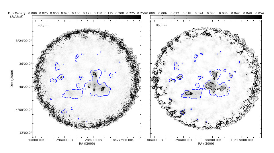
Figure 1: SCUBA-2 450 $\micron$ (left) and 850 $\micron$ (right) data. Contours show 5$\sigma$ and 15$\sigma$ levels in both cases: levels are at 0.082, 0.25 Jy/ 4^′′ pixel and 0.011, 0.033 Jy/ 6^′′ pixel at 450 µm and 850 µm respectively. The blue outer contour shows the data reduction mask for the region, based on Herschel 500 $\micron$ observations. Noise levels increase towards the edges of the map on account of the mapping method outlined in Section 2.1.

The temperature of star-forming regions has been observed and calculated using a variety of different methods and data. Some methods utilise line emission from the clouds: for example, Ladd et al. (1994) and Curtis et al. (2010) examine the CO excitation temperature and Huttemeister et al. (1993) looked at a multilevel study of ammonia lines. Often temperature assumptions are made in line with models of Jeans instability and Bonnor-Ebert Spheres (Ebert, 1955; Bonnor, 1956; Johnstone et al., 2000). An alternative method is to fit a single temperature greybody model to an observed Spectral Energy Distribution (SED) of dust continuum emission for the YSO (Hildebrand, 1983); however, this method is sensitive to the completeness of the spectrum, the emission models and local fluctuations in dust properties (Könyves et al., 2010; Bontemps et al., 2010).

Where multiple submillimetre observations exist, low temperatures (less than 20 K), which favour cloud collapse, can be inferred by the relative intensity of longer wavelengths over shorter wavelengths. For example, Herschel provides FIR and submillimetre data through PACS bands 70 $\micron$, 100 $\micron$ and 160 $\micron$ and SPIRE bands 250 $\micron$, 350 $\micron$ and 500 $\micron$ (Pilbratt et al., 2010). Men’shchikov et al. (2010); André et al. (2010) use Herschel data to construct a low resolution temperature map for the Aquila and Polaris region through fitting a greybody to dust continuum fluxes (an opacity-modified blackbody spectrum). Herschel data offers five bands of FIR and submillimetre observations and low noise levels; however, it lacks the resolution of the JCMT which can study structure on a scale of 7.9^′′(450 $\micron$) and 13.0^′′(850 $\micron$) (Dempsey et al., 2013) as opposed to 25.0^′′ and larger for 350 $\micron$ or greater submillimetre wavelengths. Sadavoy et al. (2013) combine Herschel and SCUBA-2 data to constrain both $\beta$ and temperature.

This work develops a method which takes the ratio of fluxes at submillimetre wavelengths when insufficient data points exist to construct a complete SED. The ratio method allows the constraint of temperature or $\beta$, but not both simultaneously. Throughout this paper we used a fixed $\beta$. The value and justification for this are discussed in Section 3. Similar methods have been applied by Wood et al. (1994), Arce & Goodman (1999) and Font et al. (2001) and used by Kraemer et al. (2003) at 12.5 $\micron$ and 20.6 $\micron$ and by Schnee et al. (2005) at 60 $\micron$ and 100 $\micron$. Mitchell et al. (2001) first used 450 $\micron$ and 850 $\micron$ fluxes from SCUBA, though full analysis was limited by the quality and quantity of 450 $\micron$ data. A more rigorous analysis of SCUBA data was completed by Reid & Wilson (2005) who are able to constrain errors on the temperature maps from sky opacity and the error beam components. Most recently similar methods have been used by Hatchell et al. (2013) to analyse heating in NGC1333. This work looks to utilise these methods to further investigate radiative feedback in star-forming regions.

This study uses data from the JCMT Gould Belt Survey (GBS) of nearby star-forming regions (Ward-Thompson et al., 2007). The survey maps all major low and intermediate-mass star-forming regions within 0.5 kpc. The JCMT GBS provides some of the deepest maps of star forming regions where $A_{v}>3$ with a target sensitivity of 3 mJy beam^-1 at 850 $\micron$ and 12 mJy beam^-1 at 450 $\micron$. The improved resolution of the JCMT also allows for more detailed study of large scale structures such as filaments, protostellar envelopes, extended cloud structure and morphology down to the Jeans length.

This paper focuses on the Serpens MWC 297 region, a region of low mass star formation associated with the B star MWC 297 and part of the larger Serpens-Aquila star forming complex. The exact distance to the star MWC 297 is a matter of debate. Preliminary estimates of the distance to the star were put at $450\hbox{ pc}$ by Canto et al. (1984) and $530\pm 70\hbox{ pc}$ by Bergner et al. (1988). Drew et al. (1997) used a revised spectral class of B1.5Ve to calculate a closer distance of $250\pm 50\hbox{ pc}$ which is in line with the value of $225\pm 55\hbox{ pc}$ derived by Straižys et al. (2003) for the minimum distance to the extinction wall of the whole Serpens-Aquila rift of which the star MWC 297 is thought to be a part. The distance to the Serpens-Aquila rift was originally put at a distance of $250\pm 50\hbox{ pc}$ due to association with Serpens Main, a well constrained star forming region the north of MWC 297; however, recent work by Dzib et al. (2010, 2011) has placed Serpens Main at $429\pm 2\hbox{ pc}$ using parallax. Maury et al. (2011) argues that previous methods measured the foreground part of the rift and that Serpens Main is part of a separate star forming region positioned further back. On this basis, we adopt a distance of $d=250\pm 50\hbox{ pc}$ to the Aquila rift and the Serpens MWC 297 region (Sandell et al., 2011).

The star MWC 297 is an isolated, intermediate mass Zero Age Main Sequence (ZAMS) star at RA(J2000) = $18^{h}$ $27^{m}$ $40^{s}.6$, Dec. (J2000) = $-03^{\circ}$ $50^{\prime}$ 11^′′. Drew et al. (1997) noted that MWC 297 has strong reddening due to foreground extinction ($A_{V}$ = 8) and particularly strong Balmer line emission. The star has been much studied as an example of a classic Herbig AeBe star, defined by Herbig (1960), Hillenbrand et al. (1992) and Mannings (1994) as an intermediate mass (1.5 to 10 $M_{\odot}$) equivalent of classical T-Tauri star, typically a Class III pre-main sequence star of spectral type A or B.

Herbig AeBe stars are strongly associated with circumstellar gas and dust with a wide range of temperatures. Berrilli et al. (1992) and Di Francesco et al. (1994, 1998) find evidence of an extended disk/circumstellar envelope around the star MWC 297. Radio observations constrain disk size to $<100$ AU and also find evidence for free-free emission at the poles that suggest the presence of polar winds or jets (Skinner et al., 1993; Malbet et al., 2007; Manoj et al., 2007). MWC 297 is in a loose binary system with an A2 star, hereafter referred to as OSCA, which has been identified as a source of X-ray emission (Vink et al., 2005; Damiani et al., 2006). There is evidence for an optical nebulae, SH2-62, which is coincident with MWC 297 (Sharpless, 1959).

This paper is structured as follows. In Section 2 we describe the observations of the Serpens MWC 297 region by SCUBA-2 and Spitzer. In Section 3 we apply our method for producing temperature maps from the flux ratio and asses possible sources of contamination of the submillimetre data. In Section 4 we identify clumps in the region and calculate masses. In Section 5 we examine external catalogues of YSO candidates for the region and produce our own SCUBA-2 catalogue of star-forming cores. In Section 6 we discuss our findings in the context of radiative feedback and global star formation within the region and ask if there is any evidence that radiative feedback from previous generations of stars is influencing present day and future star formation.

2 Observations and Data Reduction

2.1 SCUBA-2

Serpens MWC 297 was observed with SCUBA-2 (Holland et al., 2013) on the 5th and 8th of July 2012 as part of the JCMT Gould Belt Survey (GBS, Ward-Thompson et al. 2007) MJLSG33 SCUBA-2 Serpens Campaign (Holland et al., 2013). One scan was taken on the 5th at 12:55 UT in good Band 2 with 225 GHz opacity $\tau_{\mathrm{225}}=0.04-0.06$. Five further scans taken on the 8th between 07:23 and 11:31 UT in poor Band 2, $\tau_{\mathrm{225}}=0.07-0.11$.

Continuum observations at 850 $\micron$ and 450 $\micron$ were made using fully sampled 30^′ diameter circular regions (PONG1800 mapping mode, Chapin et al. 2013) centered on RA(J2000) = $18^{h}$ $28^{m}$ $13^{s}.8$, Dec. (J2000) = $-03^{\circ}$ $44^{\prime}$ 1.7^′′.

The data were reduced using an iterative map-making technique (makemap in smurf, Chapin et al. 2013, Jenness et al. 2013), and gridded to 6^′′ pixels at 850 $\micron$, 4^′′ pixels at 450 $\micron$. The iterations were halted when the map pixels, on average, changed by $<$0.1 per cent of the estimated map rms. The initial reductions of each individual scan were coadded to form a mosaic from which a signal-to-noise mask was produced for each region. This was combined with Herschel 500 $\micron$ emission at greater than 2 Jy/beam to include all potential emission regions. The final mosaic was produced from a second reduction using this mask to define areas of emission. Detection of emission structure and calibration accuracy are robust within the masked regions, and are uncertain outside of the masked region. The reduced map and mask are shown in Figure 1.

A spatial filter of 600^′′ is used in the reduction, which means that flux recovery is robust for sources with a Gaussian Full Width Half Maximum (FWHM) less than 2.5^′. Sources between 2.5^′ and 7.5^′ will be detected, but both the flux and the size are underestimated because Fourier components with scales greater than 5^′ are removed by the filtering process. Detection of sources larger than 7.5^′ is dependent on the mask used for reduction.

The data presented in Figure 1 are initially calibrated in units of pW and are converted to Jy per pixel using Flux Conversion Factors (FCFs) derived by Dempsey et al. (2013) from the average values of JCMT calibrators. By correcting for the pixel area, it is possible to convert maps of units Jy/pixel to Jy/beam using

$$S_{\textup{beam}}=S_{\textup{pixel}}\frac{\textup{FCF}_{\textup{peak}}}{\textup{FCF}_{\textup{arcsec}}}\frac{1}{\textup{Pixel area}}.$$ (1)

FCF_arcsec = 2.34$\pm$0.08 and 4.71$\pm$0.5 Jy/pW/arcsec², at 850 $\micron$ and 450 $\micron$ respectively, and FCF_peak = 537$\pm$26 and 491$\pm$67 Jy/pW at 850 $\micron$ and 450 $\micron$ respectively. The PONG scan pattern leads to lower noise in the map centre and overlap regions, while data reduction and emission artefacts can lead to small variations in the noise over the whole map. Typical noise levels were 0.0165 and 0.0022 Jy per pixel at 450 $\micron$ and 850 $\micron$ respectively.

The JCMT beam can be modelled as two Gaussian components (Drabek et al., 2012; Dempsey et al., 2013). The primary (or main) beam contains the bulk of the signal and is well described by a Gaussian, $G_{\mathrm{MB}}$, but in addition to this there is also a secondary beam which is much wider and lower in amplitude, $G_{\mathrm{SB}}$. Together they make up the 2-component beam of the telescope,

$$G_{\mathrm{total}}=aG_{\mathrm{MB}}+bG_{\mathrm{SB}},$$ (2)

where $a$ and $b$ are relative amplitude, listed in Table 1 alongside the FWHM, $\theta$, of the primary (MB) and secondary (SB) beams.

Table 1: JCMT beam properties

	450 $\micron$	850 $\micron$
$\theta_{\mathrm{MB}}$	7.9′′	13.0′′
$\theta_{\mathrm{SB}}$	25.0′′	48.0′′
$a$	0.94	0.98
$b$	0.06	0.02
Pixel size	4′′	6′′

JCMT beam Full Width Half Maximum ($\theta$) and relative amplitudes from Dempsey et al. (2013) Table 1. Pixel sizes are those chosen by the JCMT SGBS data reduction team.

2.2 Spitzer catalogues

Table 2: A sample of Spitzer YSO candidates (YSOc) from the SGBS. The full version appears as supplementary material online.

ID	SSTgbs	Spitzer IRAC				Spitzer MIPS
		$S_{\mathrm{3.6}}$	$S_{\mathrm{4.5}}$	$S_{\mathrm{5.8}}$	$S_{\mathrm{8.0}}$	$S_{\mathrm{24}}$	$S_{\mathrm{70}}$	$\alpha_{\mathrm{IR}}$
		mJy	mJy	mJy	mJy	mJy	mJy
YSOc2	J18271323-0340146	$193.0\pm 10.4$	$220.0\pm 11.3$	$258.00\pm 13.40$	$354.00\pm 17.20$	$1170.0\pm 110.0$	$1610\pm 172$	$-0.17$
YSOc11	J18272664-0344459	$76.2\pm 3.7$	$87.4\pm 4.5$	$92.30\pm 4.33$	$116.00\pm 6.00$	$198.0\pm 18.4$	$312\pm 41$	$-0.49$
YSOc15	J18273641-0349133	$5.4\pm 0.3$	$3.5\pm 0.2$	$10.60\pm 1.77$	$38.60\pm 8.78$	$107.0\pm 28.4$	…	$0.03$
YSOc16	J18273671-0350047	$11.0\pm 0.6$	$16.7\pm 0.9$	$24.10\pm 2.55$	$29.00\pm 2.68$	$340.0\pm 84.2$	…	$0.75$
YSOc17	J18273710-0349386	$868.0\pm 43.7$	$985.0\pm 52.2$	$1100.00\pm 57.60$	$1230.00\pm 67.20$	$1780.0\pm 262.0$	…	$-0.43$
YSOc21	J18273921-0348241	$1.0\pm 0.3$	$1.3\pm 0.1$	$10.90\pm 1.48$	$38.70\pm 7.55$	$73.5\pm 15.2$	…	$1.51$
YSOc38	J18275223-0344173	$0.1\pm 0.0$	$0.0\pm 0.0$	$0.14\pm 0.05$	$0.38\pm 0.11$	$3.8\pm 1.2$	$454\pm 195$	$1.17$
YSOc32	J18275019-0349140	$44.2\pm 2.2$	$63.7\pm 3.1$	$84.40\pm 4.01$	$96.70\pm 4.79$	$427.0\pm 39.6$	…	$0.17$
YSOc41	J18275472-0342386	$153.0\pm 7.7$	$254.0\pm 12.7$	$370.00\pm 17.80$	$571.00\pm 27.20$	$2100.0\pm 202.0$	$3480\pm 446$	$0.56$
YSOc47	J18280541-0346598	$11.9\pm 0.6$	$37.0\pm 1.9$	$59.80\pm 2.80$	$70.10\pm 3.36$	$344.0\pm 32.1$	$3560\pm 386$	$0.96$
YSOc73	J18290545-0342456	$4.7\pm 0.2$	$14.2\pm 0.7$	$21.80\pm 1.04$	$25.00\pm 1.20$	$49.4\pm 4.6$	$662\pm 71$	$0.30$

The MWC 297 region was observed twice by Spitzer in the mid-infrared, first as part of the Spitzer Young Clusters Survey (SYC; Gutermuth et al. 2009) and secondly as part of the Spitzer legacy program “Gould’s Belt: star formation in the solar neighbourhood” (SGBS, PID: 30574).

In both surveys, mapping observations were taken at 3.6, 4.5, 5.8 and 8.0 µm with the Infrared Array Camera (IRAC; Fazio et al. 2004) and at 24 µm with the Multiband Imaging Photometer for Spitzer (MIPS; Rieke et al. 2004). The SGBS also provided MIPS 70 and 160 µm coverage, although the latter saturates towards MWC 297. The IRAC observations have an angular resolution of 2^′′ whereas MIPS is diffraction limited with 6^′′, 18^′′ and 40^′′ resolution at 24, 70 and 160 µm respectively.

The SYC targeted 36 young, nearby, star-forming clusters. Specifically, a 15^′ $\times$ 15^′ area centred on the star MWC 297 was observed as part of this survey. Observations, data reduction and source classification were carried out using ClusterGrinder as described in Gutermuth et al. (2009).

The SGBS program aimed to complete the mapping of local star formation started by the Spitzer “From Molecular Cores to Planet-forming Disks” (c2d) project (Evans et al., 2003, 2009) by targeting the regions IC5146, CrA, Scorpius (renamed Ophiuchus North), Lupus II/V/VI, Auriga, Cepheus Flare, Aquila (including MWC 297), Musca, and Chameleon to the same sensitivity and using the same reduction pipeline (Gutermuth et al., 2008; Harvey et al., 2008; Kirk et al., 2009; Peterson et al., 2011; Spezzi et al., 2011; Hatchell et al., 2012). The Serpens MWC 297 region was mapped as part of the Aquila rift molecular cloud that also includes the Serpens South cluster (Gutermuth et al., 2008) and Aquila W40 regions. The observational setup, data reduction and source classification used the c2d pipeline as described in detail in Harvey et al. (2007), Harvey et al. (2008), Gutermuth et al. (2008) and the c2d delivery document (Evans et al., 2007).

As a result of these two Spitzer survey programmes, two independent lists of Young Stellar Object candidates (YSOc) exist for the MWC 297 region. We refer to Gutermuth et al. (2009) for the SYC observations and SGBS for the Spitzer Gould’s Belt survey. The SGBS catalogue (Table 2) covers the entire region mapped by SCUBA-2 whereas the SYC extent is 15^′ $\times$ 15 ^′ around MWC 297. YSOc from these methods are revisited in Section 5.1.

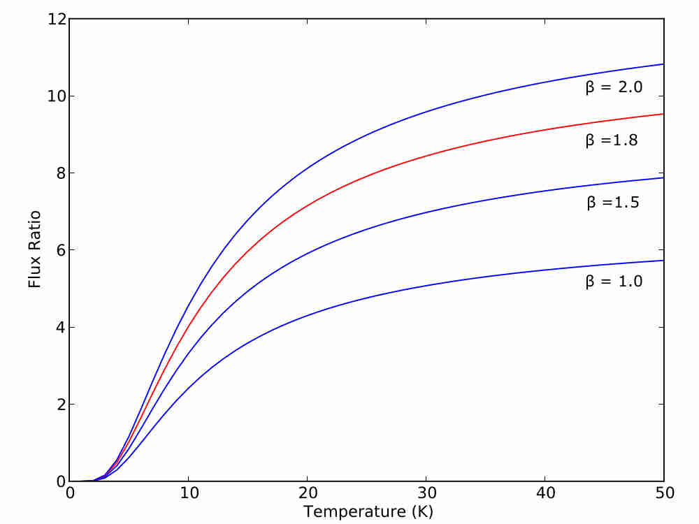
Figure 2: Flux ratio as a function of temperature as described by Equation 3. The temperature range is that commonly observed in protostellar cores.

3 Temperature mapping

Using the ratio of 450 $\micron$ and 850 $\micron$ fluxes from SCUBA-2, we develop a method that utilises the two frequency observations of the same region where the ratio depends partly on the dust temperature ($T_{\mathrm{d}}$) via the Planck function and also on the dust opacity spectral index, $\beta$ (a dimensionless term dependent on the grain model as proposed by Hildebrand 1983), as described by

$$\frac{S_{\mathrm{450}}}{S_{\mathrm{850}}}=\left(\frac{850}{450}\right)^{3+\beta}\left(\frac{\exp(hc/\lambda_{\mathrm{850}}k_{\mathrm{B}}T_{\mathrm{d}})-1}{\exp(hc/\lambda_{\mathrm{450}}k_{\mathrm{B}}T_{\mathrm{d}})-1}\right),$$ (3)

otherwise referred to as ‘the temperature equation’ (Reid & Wilson, 2005).

Temperature is known to influence the process by which dust grains coagulate and form icy mantles and therefore the value of $\beta$. Observations by Ubach et al. (2012) have shown decreases in $\beta$ in protoplanetary disks but for the most part there is little evidence that $\beta$ changes significantly in pre/protostellar cores (Schnee et al., 2014). Sadavoy et al. (2013) fitted Herschel 160 $\micron$ to 500 $\micron$ data with SCUBA-2 data in the Perseus B1 region and concluded that $\beta$ is approximately 2.0 in extended, filamentary regions whereas it takes a lower value of approximately 1.6 towards dense protostellar cores.

Figure 2 describes how small changes in $\beta$ lead to a large range of flux ratios, especially at higher temperatures. For ratios of 3, 7 and 9, a $\beta$ of 1.6 would return temperatures of 8.9, 25.4 and 85 K whereas a $\beta$ of 2.0 would return temperatures of 7.6, 15.7 and 25 K. Higher ratios indicate heating above that available from the Interstellar Radiation Field (ISRF) for any reasonable value of $\beta$.

Removing the requirement for the uncertainty in $\beta$ requires data at additional wavelengths, for example 250 $\micron$ and 350 $\micron$ as observed by Herschel. Reconciling the angular scales of Herschel observations with those of SCUBA-2 is a non-trivial process and goes beyond the scope of this paper.

Smaller values of $\beta$ are found to be consistent with grain growth which only occurs sufficiently close to compact structures (Ossenkopf & Henning, 1994). Stutz et al. (2010) used the dominance of extended structure to that of compact structure to argue for a uniform, higher value of $\beta$. Likewise Hatchell et al. (2013) assumed a constant $\beta$, arguing that variation in temperature dominates to that of $\beta$ in NGC1333. On this basis we adopt a uniform $\beta$ of 1.8, a value consistent with the popular OH5 dust model proposed by Ossenkopf & Henning (1994) and studies of dense cores with Planck, Herschel and SCUBA-2 (Stutz et al., 2010; Juvela et al., 2011; Sadavoy et al., 2013). We note that in this regime an apparent fall in temperature towards the centre of a core might be symptomatic of low $\beta$ values and therefore we cannot be as certain about the temperatures at these points.

There is no analytical solution for temperature and so pixel values are inferred from a lookup table. The method by which temperature maps are made can be split into two distinct parts: creating maps of flux ratio from input 450 $\micron$ and 850 $\micron$ data and building temperature maps based on the ratio maps. Both methods were discussed by Hatchell et al. (2013), for here on referred to as the H13 method. We focus on the development of this method and the additional features that have been incorporated.

3.1 Ratio maps

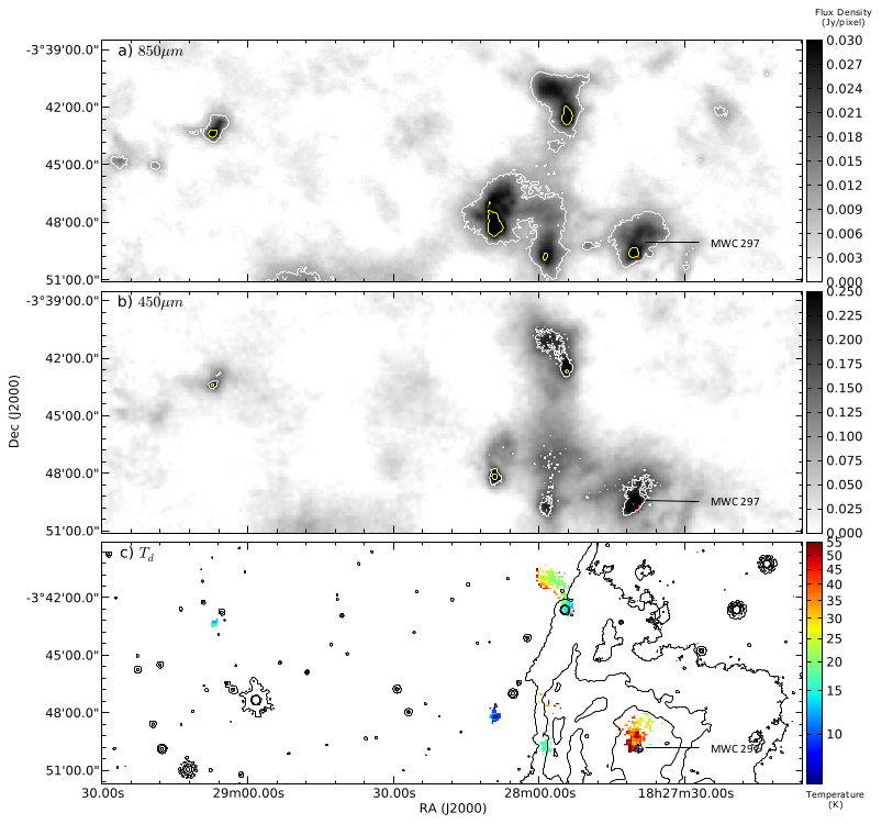
Figure 3: Top to bottom: a) SCUBA-2 convolved 850 $\micron$ flux map of Serpens MWC 297. Contours from the original 850 $\micron$ data are at 0.011, 0.033 Jy/pixel (corresponding to 5 and 15 $\sigma$). b) SCUBA-2 convolved and aligned 450 $\micron$ flux map of Serpens MWC 297 in Jy/pixel. Contours from the original 450 $\micron$ data are at 0.082, 0.25 Jy/pixel (corresponding to 5 and 15 $\sigma$). The crosses in a) and b) mark the location of the ZAMS B1.5Ve star MWC 297 and its binary partner OSCA (A2v). c) Dust temperature map of Serpens MWC 297 for $\beta$ = 1.8. Contours of Spitzer 24 $\micron$ emission at 32, 40 and 70 MJy per Sr are overlaid.

Free parameters of our method are limited to $\beta$ (which we set at 1.8). Input 450 $\micron$ and 850 $\micron$ flux density data (scaled in Jy/pixel) have fixed noise levels. Other fixed parameters which are used in the beam convolution include: the pixel area per map, FWHM of the primary ($\theta_{\mathrm{MB}}$) and secondary ($\theta_{\mathrm{SB}}$) beams and beam amplitudes all of which are measured by Dempsey et al. (2013) and given in Table 1.

Input maps are first convolved with the JCMT beam (Equation 1) at the alternate wavelength to match resolution. Pixel size is taken into account in this process. The 450 $\micron$ fluxes are then regridded onto the 850 $\micron$ pixel grid. Data are then masked leaving only 5$\sigma$ detections or higher. 450 $\micron$ fluxes are then divided by 850 $\micron$ fluxes to create a map of flux ratio.

Whereas the H13 method made a noise cut based on the variance array calculated during data reduction, our model introduces a cut based on a single noise estimate, following the method introduced by Salji (2014). The data are masked to remove pixels which carry astronomical signal. The remaining pixels are placed in a histogram of intensity and a Gaussian is fitted to the distribution, from which a standard deviation, $\sigma$, can be extracted as the noise level. This calculation is a robust form of measuring statistical noise that includes residual sky fluctuations.

We introduce a secondary beam component into the H13 method, which previously assumed that the secondary component was negligible. This adds complexity to the convolution process as it requires convolution of the data with a normalised Gaussian of the form of the JCMT beam’s primary and secondary components for the alternative wavelength. The primary component at 850 µm is then scaled with

$$\frac{a_{\mathrm{450}}\theta_{\mathrm{MB_{\mathrm{450}}}}^{2}}{a_{\mathrm{450}}\theta_{\mathrm{MB_{\mathrm{450}}}}^{2}+b_{\mathrm{450}}\theta_{\mathrm{SB_{\mathrm{450}}}}^{2}},$$ (4)

and likewise

$$\frac{b_{\mathrm{450}}\theta_{\mathrm{SB_{\mathrm{450}}}}^{2}}{a_{\mathrm{450}}\theta_{\mathrm{MB_{\mathrm{450}}}}^{2}+b_{\mathrm{450}}\theta_{\mathrm{SB_{\mathrm{450}}}}^{2}},$$ (5)

for the secondary component. The 450 $\micron$ map is convolved with the 850 $\micron$ beam is a similar way. Corresponding parts are then summed together for 450 $\micron$ and 850 $\micron$ data separately to construct the convolved maps with an effective beam size of 19.9^′′ as shown in Figure 3.

The inclusion of the secondary beam was found to decrease temperatures by between 5 per cent and 9 per cent with the coldest regions experiencing the largest drop in temperature and warmest the least.

Applying a 5$\sigma$ cut based on the original 450 $\micron$ data to mask uncertain regions of large scale structure after the beam convolution can lead to spuriously high values around the edges of our maps where fluxes from pixels below the threshold are contributing to those above, producing false positives. These ‘edge effects’ are mitigated by clipping but we advise that where the highest temperature pixels meet the map edges these data be regarded with a degree of scepticism.

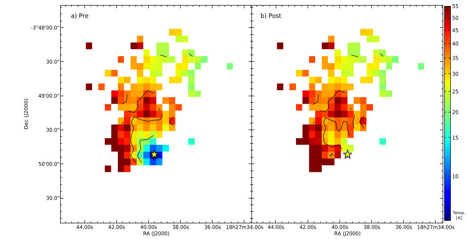
Figure 4: Temperature maps of MWC 297 from the ratio of 450 $\micron$ and 850 $\micron$ emission pre (left) and post (right) free-free contamination subtraction. Contours are at 11, 25 and 38 K. The location of MWC 297 is marked with a star.

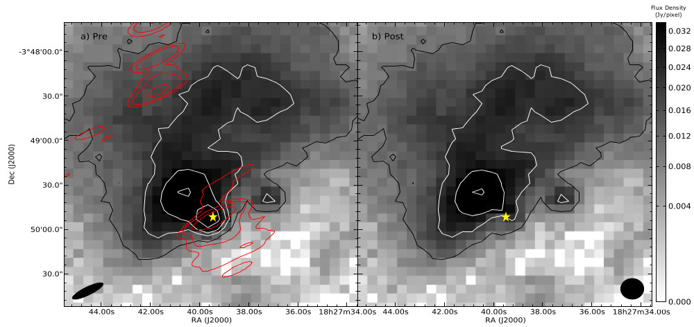
Figure 5: IR1 SCUBA-2 850 $\micron$ data before left and after right removal of free-free contamination from an UCHII region and polar jets/winds (represented by the point source contours in the left plot). SCUBA-2 contours are at 0.011, 0.022, 0.033 and 0.055 Jy/pixel (corresponding to 5, 10, 15 and 25 $\sigma$ detection limits). 6 cm VLA contours (red) from Sandell (private comm.) at 0.002, 0.005, 0.02, 0.072, 0.083 Jy/beam are overlaid on the left hand panel. The location of MWC 297 is marked with a star. Beam sizes are shown at the bottom of the image (VLA CnD config. left and JCMT right.)

3.2 Dust temperature maps

Ratio maps are converted to temperature maps using Equation 3 implemented as a look-up table as there is no analytical solution. The H13 method subsequently cuts pixels with an arbitrary uncertainty in temperature of greater than 5.5 K. We replace this with a cut of pixels of an uncertainty in temperature (calculated from the noise level propagated through the method described in Section 3.1) of greater than 5 per cent.

The 450 $\micron$ and 850 $\micron$ SCUBA-2 data for the MWC 297 region are presented in Figure 3 alongside a map of temperature of submillimetre dust in that region. These maps show a large diversity in temperature across five isolated regions of significant flux (shown in Figure 3c). Mean cloud temperatures range from 10.1$\pm$0.9 K and 15$\pm$2 K for regions which are relatively cold and isotropic, to 25$\pm$17 K for warmer regions with a large diversity of temperatures. Figure 4 shows one cloud that has a temperature of 41$\pm$19 K which is hot to the extent that this would suggest an active heat source. The range in temperatures suggests that the regions within the Serpens MWC 297 vary in physical conditions.

Men’shchikov et al. (2010) infer temperature variation from contrasting strengths of 350 $\micron$ flux bands to the shorter 70 $\micron$ and 160 $\micron$ bands of Herschel. They quote a temperature range for dense, starless filaments of 7.5 to 15 K across the whole Aquila rift. However, we do not observe a typical filamentary structure in Serpens MWC 297 region (Figure 1).

Könyves et al. (2010) and Bontemps et al. (2010) used single-temperature modified black-body fitting of SEDs of Herschel 500 $\micron$ data points in Aquila and Polaris. Their study includes Serpens MWC 297 and they find temperatures for the region ranging between 24 and 26 K. Though Herschel 500 $\micron$ data is at a lower resolution than our effective beam, the general temperatures of the region seem consistent with our findings.

Hatchell et al. (2013) use only the primary beam to study NGC1333, finding typical dust temperatures of ranging from 12 to 16 K. They also argue for a heated region pushing temperatures up as high as 35 to 40 K near the location of the B star SVS3. When the moderating effects of the secondary beam are taken into account, these results are largely consistent with our findings (Serpens MWC 297 also contains a B star).

Figure 3c shows Spitzer MIPS 24 $\micron$ flux for the Serpens MWC 297 region. These data show hot compact sources associated with individual stellar cores. It also shows the morphology of an extended IR nebulosity, associated with SH2-62, that is centred on MWC 297. As well as the dust within the immediate vicinity of the star MWC 297 showing clear signs of heating, we observe 24 $\micron$ emission that is coincident with heating in the SCUBA-2 temperature maps. As 24 $\micron$ emission provides independent evidence of heating, where we observe high temperature pixels that are not coincident with 24 $\micron$ emission (for example in the northernmost cloud) we conclude we are likely witnessing data reduction artefacts as opposed to warm gas and dust.

In addition to providing evidence for direct heating by MWC 297, the 24 $\micron$ data also provide strong evidence that the B star is physically connected to the observed clouds. The Aquila rift is thought to be a distance of 250$\pm$50 pc (Maury et al., 2011) and through association we conclude that the distance to MWC 297 matches this figure.

3.3 Contamination

Reliable temperatures depend on accurate input fluxes. Systematic contamination of 450 $\micron$ and 850 $\micron$ flux by molecular lines, in particular CO, is a known problem within SCUBA-2 data (Drabek et al., 2012). We investigate the contribution of CO and free-free emission to these bands and attempt to mitigate their effects where necessary.

Hatchell et al. (2013) and Drabek et al. (2012) highlighted 345 GHz contamination of 850 $\micron$ due to the CO 3–2 line in other Gould Belt star-forming regions. Limited ¹²CO and ¹³CO 1–0 data exist for the Serpens MWC 297 region (Canto et al., 1984). A very rough estimate of the CO contamination towards the star MWC 297 can be made based on the published spectra. The ¹²CO lines are broad ($\sim 12~{}\hbox{ km s}^{-1}$) but do not show line wings characteristic of outflows. Making the simplest assumption that the ¹²CO is optically thick and fills the beam in both the $J=1\hbox{--}0$ and $J=3\hbox{--}2$ lines, the integrated intensity of the latter will be similar to the former, $\sim 36\,\hbox{K km s}^{-1}$, corresponding to a CO contamination of 1.14 mJy/pixel/K km^-1 (13 per cent of peak flux) at the position of the star MWC 297 using the conversion in Drabek et al. (2012) updated for the beam parameters in Dempsey et al. (2013). Drabek et al. (2012) noted than regions where CO emission accounts for less that 20 per cent of total peak emission are not consistent with outflows or major contamination. Manoj et al. (2007) find no evidence of CO 2–1 and ${}^{13}\textrm{CO~{}2\hbox{--}1}$ emission within 80 AU of MWC 297 and conclude this depletion is caused by photoionisation due to an ultra-compact HII (UCHII) region as has been detected by Drew et al. (1997) and Malbet et al. (2007).

The inferred presence of an UCHII region has consequences for contamination at submillimetre wavelengths through thermal bremsstrahlung, or free-free emission, from ionised gas with temperatures of 10,000 K or higher. Free-free emission is optically thick at the longest wavelengths and has a relatively flat power law in the optically thin regime at radio and far infrared wavelengths before undergoing exponential cut off at shorter wavelengths. Skinner et al. (1993) studied free-free 3.6 cm and 6.0 cm radio emission from stellar winds around MWC 297 and found a power law of the form $S_{\nu}\propto\nu^{\alpha}$ where $\alpha$ is equal to 0.6238 in the optically thin regime. Sandell et al. (2011) extended the study down to 3 mm and revised the spectral index to $\alpha=1.03\pm 0.02$ which is consistent with a collimated jet component to free-free emission. The free-free power law extends into the submillimetre spectrum; however, at wavelengths shorter than 2.7 mm there is potential for a thermal dust component in the observed flux, so submillimetre flux is not included in the calculation of $\alpha$.

Figure 5 displays 6 cm radio emission from the VLA CnD configuration in conjunction with SCUBA-2 850 $\micron$ data (Skinner 1993, Sandell priv. comm). Both sets of data show peaks in emission which are coincident with a point source at the location of the star MWC 297 in 1 mm and 3 mm data presented by Alonso-Albi et al. (2009). The peak of the SCUBA-2 850 $\micron$ emission in Figure 5 is 86 mJy/pixel, consistent with the SCUBA 850 $\micron$ value of 82 mJy/pixel (Alonso-Albi et al., 2009).

The VLA data also show extended emission to the north and south of MWC 297 which is consistent with polar winds or jets. The intensity of emission is significantly weaker than that of the UCHII region. Considering the elongated beam shape of the VLA CnD observations (21.1^′′$\times$ 5.2^′′, PA$=-61^{\circ}.3$) accounts for much the E/W elongation of the emission. In addition to this, Manoj et al. (2007) describe this emission as coming from within 80 AU of MWC 297. This is much smaller than the JCMT beam and therefore we model the dominant free-free emission from MWC 297 as a point source.

By taking the revised power law least square fit to Skinner et al. (1993) and Sandell et al. (2011)’s results at radio and milimetre wavelengths and extrapolating to the submillimetre wavelengths of SCUBA-2, we are able to calculate the effect of free-free emission due to a point-like UCHII region as an integrated flux of 934$\pm$128 mJy at 450 $\micron$ and 471$\pm$62 mJy at 850 $\micron$. By convolving this point with the JCMT beam we find that free-free contamination corresponds to approximately 73$\pm$5 per cent and 82$\pm$4 per cent of the 450 $\micron$ and 850 $\micron$ peak flux respectively in the case of MWC 297. Residual dust peak fluxes are $51\pm 10$ mJy and $15\pm 3$ mJy flux per pixel at 450 $\micron$ and 850 $\micron$ respectively and are highlighted in Figure 6 as the flux above the free-free power law fit of $\alpha=1.03\pm 0.02$. Given our estimate of 13 per cent CO contamination, dust emission could potentially account for as little as 5 per cent of peak emission at 850 $\micron$.

We cannot say whether any dust emission contributes at the position of MWC 297. Figure 5 presents the 850 $\micron$ before and after subtraction. Figure 4 presents the impact of free-free emission on temperature maps of the region. Even with the free-free emission subtracted, a large, extended submillimetre clump remains, though its peak is offset from the location of MWC 297 by 24.2^′′ (approximately 6,000 AU).

The impact of this contamination on the temperature maps is remarkable. The power law of $\alpha=1.03\pm 0.02$ that describes free-free emission from both an UCHII region and jet outflows produces greater flux at 850 $\micron$ than 450 $\micron$. Free-free dominates the flux and this results in artificially lower ratios and therefore lower temperatures. This is consistent with the cold spot seen in Figure 4a at the location of the UCHII region, with a temperature of approximately 11 K. We can conclude that free-free emission may contaminate submillimetre temperature maps where cold spots are coincident with hot OB stars.

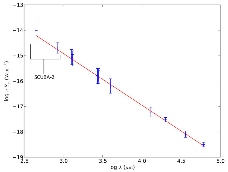
Figure 6: The Spectral Energy Distribution of MWC 297 from submillimetre to radio wavelengths. SCUBA-2 fluxes (found using aperture photometry as described in Section 5.2.) are presented alongside those collated by Sandell et al. (2011) who fit a power law $\alpha=1.03\pm 0.02$, consistent with free-free emission from an UCHII region and polar jets or outflows.

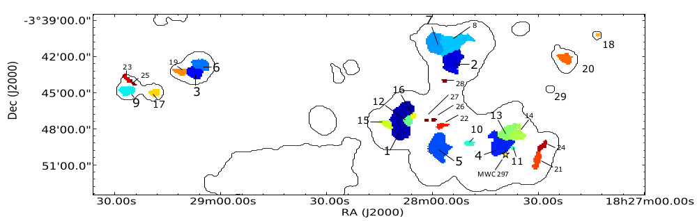
Figure 7: Clumps identified in 850 $\micron$ data with the starlink clump-finding algorithm fellwalker index numbered in order (highest to lowest following the colour scale) of integrated flux. The data reduction mask is overlaid as a black contour.

4 The SCUBA-2 clump catalogue

In this section we introduce the clump-finding algorithm fellwalker used to identify clumps in the SCUBA-2 data presented in Figure 1. We calculate clump masses and compare these to their Jeans masses to determine whether or not the objects are unstable to gravitational collapse.

4.1 Identification of structure

Clumps do not have well defined boundaries within the ISM. We use the signal to noise ratio to define a boundary at an effective radius. The boundary is determined by the starlink CUPID package for the detection and analysis of objects (Berry et al., 2013), specifically the fellwalker algorithm which assigns pixels to a given region based on positive gradient towards a common emission peak. This method has greater consistency over parameter space than other algorithms (Watson 2010, Barry et al. 2014, submitted). fellwalker was developed by Berry et al. (2007), and the 2D version of the algorithm used here considers a pixel in the data above the noise level parameter and then compares its value to the adjacent pixels. fellwalker then moves on to the adjacent pixel which provides the greatest positive gradient. This process continues until the peak is reached - when this happens all the pixels in the ‘route’ are assigned an index and the algorithm is repeated with a new pixel. All ‘routes’ that reach the same peak are assigned the same index and form the ‘clump’. Clump-finding algorithms, such as this, have been used by Johnstone et al. (2000), Hatchell et al. (2005), Kirk et al. (2006) and Hatchell et al. (2007) to define the extent of clumps for the purposes of measuring clump mass.

We tuned the fellwalker algorithm to produce a set of objects consistent with a by-eye decomposition, setting the following parameters; MinDip = 1$\sigma$ (minimum flux between two peaks), MinPix = 4 pixels (minimum number of pixels per valid clump), MaxJump = 1 pixel (distance between clump peaks), FWHMBeam = 0 (FWHM of instrument), MinHeight = 3$\sigma$ (minimum height of clump peak to register as a valid clump) and Noise = 3$\sigma$ (detection level). Throughout this process we used a constant noise level, $\sigma$, calculated via the method described by Salji (2014) and described in Section 3.1. Watson (2010) discusses the fellwalker parameters in depth and concludes MinDip and MaxPix are the most influential in returning the maximum breakup of clouds into clumps, a subset of which will later be used to compile a list of protostellar cores. The $3\sigma$ level allows for the detection of the smallest clumps that may be missed at the $5\sigma$ level on account of insufficient pixels for detection as outlined above. This method also included a number of spurious clumps associated with high variance pixels at the maps edges. In order to avoid these we first masked the SCUBA-2 data with the data reduction mask shown in Figure 1.

Using these parameters 28 submillimetre clumps were detected in 850 $\micron$ data and are presented in Figure 7. Two sources (SMM 23 and 25) were immediately discarded as they were not consistent with a 5$\sigma$ detection. A further two clumps were split into two separate objects by the algorithm when there was no discernible peak in the submillimetre data. In these cases (SMM 7 & 8 and SMM 13 & 14) the objects were recombined into single object. We note that this is a side effect of having a low MinDip parameter to maximise the detection of smaller clumps. In total a sample of 23 clumps are presented in Table 3. We note that there is a known bias that underestimates the size of a clump as its peak flux approaches the cutoff level and therefore biases against the detection of cold, faint objects (examples might be SMM 26 and 27). Modelling clump profiles could be used to better estimate the full extent of these objects. However, as these present a minority of cases we take no further action on this issue (Rosolowsky & Leroy, 2006).

The fellwalker algorithm is insensitive to low mass, isolated objects where detections were limited to less than five pixels above the noise level. We find that one potential source was missed on account of it only exhibiting a single significant pixel above the 5$\sigma$ noise level. Here object flux was measured with aperture photometry (see Section 5.2).

Due to the higher noise level of the 450 $\micron$ data many objects detected at 850 $\micron$ were not present at 450 $\micron$. Therefore we apply the 850 $\micron$ clump boundaries to the 450 $\micron$ data when calculating integrated intensity at that wavelength to ensure consistent flux extraction at both wavelengths for each object.

4.2 Measurement of mass

SCUBA-2 observations of the Serpens MWC 297 region were used to calculate the masses of the fellwalker clumps. Hildebrand (1983) describes how the mass of a cloud can be calculated from the submillimetre emission of dust grains fitted to a black-body spectrum for a nominal temperature. We follow this standard method for calculating clump mass (for example Johnstone et al. 2000, Kirk et al. 2006, Sadavoy et al. 2010 and Enoch et al. 2011). We use flux at 850 $\micron$ ($S_{\mathrm{850}}$) per pixel, dust opacity ($\kappa_{\mathrm{850}}$), distance ($d$) and a variable temperature ($T_{\mathrm{d}}$) per pixel, summing over all pixels, $i$, in the clump to calculate the total clump mass:

$$M =0.39\sum_{i}S_{\mathrm{850,i}}\left[\exp\left(\frac{17\mathrm{K}}{T_{\mathrm{d},i}}\right)-1\right]$$

$$\times\left(\frac{d}{250\mathrm{pc}}\right)^{2}\left(\frac{\kappa_{\mathrm{850}}}{0.012\mathrm{\hbox{cm}^{2}\hbox{g}^{-1}}}\right)^{-1}.$$

There is a high degree of uncertainty in the value of $\kappa_{\mathrm{850}}$. The popular OH5 model of opacities in dense ISM, with a specific gas to dust ratio of 161, gives 0.012 $\hbox{cm}^{2}\hbox{g}^{-1}$ at 850 $\micron$ (Ossenkopf & Henning, 1994). Comparable studies suggest values of 0.01 (Johnstone et al., 2000), 0.019 (Eiroa et al., 2008) and 0.02 $\hbox{cm}^{2}\hbox{g}^{-1}$ (Kirk et al., 2006). Henning & Sablotny (1995) find $\kappa_{\mathrm{850}}$ can vary by up to a factor of two. We assume an opacity of $\kappa_{\mathrm{850}}$ = 0.012 following Hatchell et al. (2005). This value is consistent with $\beta$ = 1.8 over a wavelength range of 30 $\micron$ to 1.3 mm. We assume a distance $d=250\pm 50\hbox{ pc}$ following Sandell et al. (2011) as outlined in Section 1.

We calculate dust masses using dust temperatures calculated for each pixel where possible. Not all the clumps shown in Figure 7 have temperature data due to the noise constraints of the temperature mapping process and the requirement that the region is also detected at 450 $\micron$. For those that do not, a constant clump temperature of 15 K is assumed following Johnstone et al. (2000) and Kirk et al. (2006). Some clumps have only partial temperature data. In these cases the remaining pixels are filled with a value equal to the mean of the existing data. In some cases (SMM 6 and 11 for example), temperature data is limited to a few pixels whereas the total clump area is an order of magnitude larger. As it is unlikely that such a small sample of data will accurately represent the whole clump, results for objects such as these should be treated with a larger degree of uncertainty. Edge effects have a negligible influence on clump mass as high temperatures reduce the contribution in Equation 5. Clump masses are listed in Table 3.

The total mass of clumps in Serpens MWC 297 is 40$\pm$3 $M_{\mathrm{\odot}}$. Individual clump masses range over 2 orders of magnitude from 0.05 to 19 $M_{\mathrm{\odot}}$ with 29 per cent of objects having a mass of 1 $M_{\mathrm{\odot}}$ or higher. Figure 7 shows how fellwalker divides the areas of star formation into five large-scale star-forming clouds and a small number of isolated objects. Of these clouds, SMM 1, 12, 15 & 16 is the most massive at 21$\pm$2 $M_{\mathrm{\odot}}$, containing 53 per cent of all the mass detected by fellwalker, followed by SMM 2, 7 & 8 at 6.6$\pm$0.3 $M_{\mathrm{\odot}}$ (17 per cent), SMM 4, 10, 11, 13, 14, 21 & 24 at 3.3$\pm$0.1 $M_{\mathrm{\odot}}$ (9 per cent), SMM 3, 6 & 19 at 3.1$\pm$0.1 $M_{\mathrm{\odot}}$ (8 per cent) and SMM 5, 22, 26 & 27 at 3.1$\pm$0.3 $M_{\mathrm{\odot}}$ (8 per cent).

Table 3: Properties of submillimetre clumps in MWC 297.

IDa	Object nameb	$S_{\mathrm{450}}^{c}$	$S_{\mathrm{850}}^{c}$	$M_{\mathrm{850}}^{d}$	$T_{\mathrm{d}}^{e}$	Areaa	$M_{\mathrm{J}}^{f}$	$M_{\mathrm{850}}/$$M_{\mathrm{J}}$	SGBS YSOc IDg
		(Jy)	(Jy)	(M${}_{\mathrm{\odot}})$	(K)	(pixels)	(M${}_{\mathrm{\odot}})$
SMM1	JCMTLSG J1828090-0349497	45.7	11.5	19(2)	10.1(0.5)	358	2.1(0.1)	9.12(1.05)	-
SMM2	JCMTLSG J1827542-0343197	33.2	5.0	3.5(0.2)	17.9(0.9)	205	2.9(0.1)	1.21(0.1)	YSOc41
SMM3	JCMTLSG J1829071-0344378	11.2	1.9	1.6(0.1)	14.6(0.7)	94	1.58(0.08)	1.03(0.1)	-
SMM4	JCMTLSG J1827405-0350257	43.9	4.7	0.91(0.05)	46(2)	213	7.4(0.4)	0.12(0.01)	-
SMM5	JCMTLSG J1827590-0350137	36.8	5.4	3.3(0.3)	18.2(0.9)	265	3.3(0.2)	0.99(0.09)	-
SMM6	JCMTLSG J1829055-0343138	7.7	1.3	1.2(0.1)	14.2(0.7)	94	1.53(0.08)	0.77(0.08)	YSOc73
SMM7*	JCMTLSG J1827586-0342557	59.4	7.7	3.1(0.2)	25(2)	419	8.2(0.3)	0.37(0.03)	-
SMM9	JCMTLSG J1829260-0345139	3.1	0.8	0.67(0.06)	15.0(-)	73	1.43(0.07)	0.47(0.05)	-
SMM10	JCMTLSG J1827501-0350437	3.5	0.4	0.29(0.03)	15.0(-)	26	0.85(0.04)	0.35(0.04)	YSOc32
SMM11	JCMTLSG J1827373-0350197	1.1	0.2	0.1(0.02)	17.6(0.9)	9	0.59(0.03)	0.17(0.03)	YSOc17
SMM12	JCMTLSG J1828074-0348437	4.1	1.0	0.86(0.07)	15.0(-)	42	1.08(0.05)	0.79(0.08)	-
SMM13*	JCMTLSG J1827393-0349257	30.9	3.8	1.25(0.06)	28(2)	199	6.3(0.2)	0.20(0.01)	-
SMM15	JCMTLSG J1828126-0348197	1.8	1.0	0.8(0.07)	15.0(-)	50	1.18(0.06)	0.68(0.07)	-
SMM16	JCMTLSG J1828058-0347017	2.2	0.4	0.33(0.03)	15.0(-)	18	0.71(0.04)	0.47(0.05)	YSOc47
SMM17	JCMTLSG J1829187-0346559	2.7	0.4	0.34(0.03)	15.0(-)	42	1.08(0.05)	0.32(0.03)	-
SMM18	JCMTLSG J1827133-0341438	0.2	0.1	0.05(0.02)	15.0(-)	7	0.44(0.02)	0.12(0.04)	YSOc2
SMM19	JCMTLSG J1829107-0344378	2.5	0.4	0.33(0.03)	15.0(-)	47	1.14(0.06)	0.29(0.03)	-
SMM20	JCMTLSG J1827225-0343378	1.4	0.7	0.61(0.05)	15.0(-)	73	1.43(0.07)	0.43(0.04)	-
SMM21	JCMTLSG J1827297-0351378	5.1	0.6	0.46(0.04)	15.0(-)	65	1.35(0.07)	0.34(0.04)	-
SMM22	JCMTLSG J1827582-0348137	4.7	0.5	0.1(0.01)	42(2)	31	2.6(0.1)	0.04(0.0)	-
SMM24	JCMTLSG J1827285-0350378	3.5	0.4	0.29(0.03)	15.0(-)	37	1.02(0.05)	0.29(0.03)	-
SMM26	JCMTLSG J1827594-0348437	1.5	0.2	0.15(0.02)	15.0(-)	10	0.53(0.03)	0.28(0.04)	-
SMM29	JCMTLSG J1828022-0348377	0.6	0.1	0.09(0.02)	15.0(-)	6	0.41(0.02)	0.23(0.05)	-

a) Clumps as identified by the fellwalker algorithm.
b) Position of the highest value pixel in each clump (at 850µm).
c) Integrated fluxes of the clumps as determined by fellwalker. The uncertainty at 450 $\micron$ is 0.3 Jy and at 850 $\micron$ is 0.02 Jy. There is an additional systematic error in calibration of 10.6 per cent and 3.4 per cent at 450 $\micron$ and 850 $\micron$.
d) As calculated with equation LABEL:eqn:mass. Errors in brackets are calculated from error in total flux, described in c., and error in mean temperature of 5 per cent. These results do not include the systematic error in distance (20 per cent) and opacity (100 per cent).
e) Mean temperature as calculated from the temperature maps (Figure 3). Where no temperature data is available an arbitrary value of 15K(-) is assigned that is consistent with the literature.
f) As calculated with equation 7. These results have a systematic error uncertainty due to distance of 20 per cent.
g) Where a fellwalker source is coincident with a SGBS YSOc, that object is listed here. A complete list is presented in Table 2.
Objects indicated with * have been merged with an adjacent object which was incorrectly identified as a separate clump by fellwalker.

4.3 Clump stability

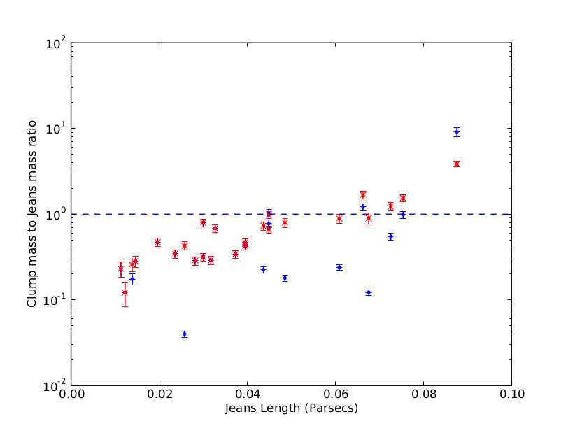
Figure 8: Jeans stability plotted against Jeans length. All clumps with $M_{\mathrm{850}}/M_{\mathrm{J}}>1$, as shown by the dashed line, are expected to be undergoing collapse. Blue circles represent calculations made with real temperature data whereas red crosses indicate those made with an assumed temperature of 15 K. Systematic error in the measurement of distance to MWC 297 accounts for 20 per cent uncertainty on Jeans length.

The Jeans instability (Jeans, 1902) describes the balance between thermal support and gravitational collapse in an idealised cloud of gas. $R_{\mathrm{J}}$ defines a critical length scale above which the cloud may collapse on a free fall timescale and star formation can take place. Analogously, $M_{\mathrm{J}}$ defines an upper limit of mass. Assuming a spherical clump has a density such that it is Jeans unstable to perturbations at the size of the clump, $R_{\mathrm{J}}$, then

$$M_{\mathrm{J}}=1.9\left(\frac{\bar{T}_{\mathrm{d}}}{10\mathrm{K}}\right)\left(\frac{R_{\mathrm{J}}}{0.07\mathrm{pc}}\right)M_{\mathrm{\odot}}.$$ (7)

We use the effective radius of the clump, as determined by clump area (in pixels) from fellwalker (Table 3), as the length scale $R_{\mathrm{J}}$. We note that effective radius is a lower limit on clump size. Mean temperature, $\bar{T}$, across the clump is calculated directly from our temperature maps.

Whereas mass was calculated on a pixel-by-pixel basis, this is not possible for $M_{J}$ as the characteristic length scale of the Jeans instability covers the entire object. Instead we use a mean temperature calculated from our maps. Temperatures and Jeans masses of clumps are also shown in Table 3. The masses of clumps calculated with the temperature data in the previous section deviates from the equivalent masses calculated with a uniform mean temperature (set at 15 K) of that clump by 12 per cent on average per clump which is sufficiently similar to allow this analysis.

This method is based on the work by Sadavoy et al. (2010) who performed a similar analysis for starless cores in the Gould belt. They used the assumption of a typical cold (10K) molecular cloud core size of 0.07 pc (Di Francesco et al., 2007). Rosolowsky et al. (2008) determined a range of temperatures of 9 K to 26 K in Perseus (a similar region to Serpens-Aquila) from ammonia observations. This paper goes a step further and is able to use mean temperatures specific to each clump. We determine a mean clump temperature of $20\pm 10$ K. The greater uncertainty on this value is indicative of the greater diversity of temperatures than assumed by Sadavoy et al. (2010).

Under the assumption that only internal pressure can balance self-gravity, $M_{J}$ sets an upper limit on the mass of a sphere of gas for a given radius. If the observed mass, $M_{850}$, is greater than the calculated $M_{J}$, or alternatively $M_{\mathrm{850}}/$$M_{\mathrm{J}}>1$, that would suggest that the clump is unstable to gravitational collapse and hence active star formation is likely (Mairs et al., 2014). An object that has $M_{\mathrm{850}}/$$M_{\mathrm{J}}\ll 1$ is currently stable and will not collapse (alternatively it has already collapsed and the majority of the mass is now contained within the protostar). Given the uncertainties present in theory and observations, the stability of objects where $M_{\mathrm{850}}/$$M_{\mathrm{J}}\approx 1$ is ambiguous. Figure  8 plots $M_{\mathrm{850}}/$$M_{\mathrm{J}}$ against the Jeans length scale for the clumps identified in Serpens MWC 297 and reveals that at least three out of a total 22 clumps detected by fellwalker are Jeans unstable and may contain protostars. Evidence for these are addressed in Section 5. For comparison, $M_{\mathrm{850}}/$$M_{\mathrm{J}}$ is plotted for the same list of objects, assuming a single clump temperature of 15 K (the red crosses in Figure 8). We observe that in a majority of cases using a real temperature has caused the ratio to decrease and we therefore conclude that previous authors who have used a constant temperature of 15 K have underestimated the stability of their clumps.

5 The SCUBA-2 Confirmed YSOc catalogue

In this section we cross-reference our list of SCUBA-2 clumps, as identified by fellwalker, with Spitzer YSOc catalogues and produce our own SCUBA-2 confirmed YSOc catalogue for the Serpens MWC 297 region.

We calculate the relative distribution of protostars to PMS stars in the region as a measure of dynamical evolution of YSOcs within a star-forming cluster. We produce Spectral Energy Distributions (SEDs) of the YSOcs where supplementary data exist. With the addition of new SCUBA-2 data at 450 $\micron$ and 850 $\micron$ we update the classification of the YSOcs in the Serpens MWC 297 region.

5.1 IR and other YSO candidates

We pull together existing YSOc catalogues, discuss the various methods used to compile them, compare the distribution of objects to the SCUBA-2 submillimetre data. From here on Class 0, I and Flat Spectrum (FS) YSOs are referred to as protostars and Class II, Transition Disk (TD) and III YSOs are referred to as Pre-Main Sequence (PMS) stars.

Three YSOc catalogues are found for the Serpens MWC 297 region, each deploying a different method to identify and classify YSOcs. The earliest catalogue found is of Chandra ACIS-I X-Ray observations carried out by Damiani et al. (2006) over an area of 16.9^′ $\times$ 8.7^′ centred on the star MWC 297. YSOc identification is a byproduct of the investigation into the X-ray flaring of the star MWC 297 and as a consequence their sample is incomplete for the whole of the Serpens MWC 297 region (30 ^′ diameter). They find that the star MWC 297 only accounts for 5.5 per cent of X-ray emission in the region. The rest is attributed to flaring low mass PMS. As Damiani et al. (2006) do not make the distinction between YSOs and more evolved objects in their work it is not possible to use these data for the purposes of classification.

SGBS and SYC (Gutermuth et al., 2009) used Spitzer observations to catalogue YSOcs for the Serpens MWC 297 region. The details of these surveys are noted in Section 2.2. SGBS used IRAC and MIPS bands to identify Class I and II detecting a total of 76 YSOcs within a 20 ^′ radius of the centre of the field (Table 2), whereas Gutermuth et al. (2009) identified 22 YSOcs using a colour-colour method, though the coverage of SYC is limited to a 15^′ square.

Where the samples overlap we find notable differences between the catalogues. SGBS include five protostars whereas SYC include four. Of these samples, only three are consistent across catalogues. These are YSOc2, 47 and 11 presented in Table 2. Similarly SGBS identifies 22 PMS-stars whereas SYC identified 18. Across the sample 11 are consistent in both catalogues. Objects that appear in both catalogues are most likely to be real YSOs.

Of the two Spitzer YSOc surveys, we use SGBS as the primary Spitzer catalogue because it covers all of the SCUBA-2 mapped area.

All IR surveys are subject to contamination by Galactic sources (for example, field red giants) and extra-Galactic sources (broad line AGN). Gutermuth et al. (2009) calculate that this should account for less than 2 per cent of sources in Serpens/Aquila. In addition to this, Connelley & Greene (2010) discuss how target inclination can play a role in classification. In Table 4 we give the total numbers of YSOcs in each catalogue by evolutionary class whilst in Figures 9 and 10 we plot the positions and evolutionary classification of the SGBS YSOcs on the 850 $\micron$ flux map. In Figure 9 we show whether or not the Spitzer YSOcs are consistent with the Damiani et al. (2006) X-ray sources.

Table 4: YSO candidates in the MWC 297 region.

	YSO Classification
	0/I	II	III
Damiani et al. (2006)	-	-	27
SGBSa - Gutermuth et al. (2008)	8	32	36
SYC - Gutermuth et al. (2009)	4	16	2
Totalb	10		72

a) Within a 20^′ radius area centred at RA(J2000) = $18^{h}$ $28^{m}$ $13^{s}.8$, Dec. (J2000) = $-03^{\circ}$ $44^{\prime}$ 1.7^′′.
b) The totals account for sources which feature in multiple catalogues.

Kaas et al. (2004), Winston et al. (2007) and Harvey et al. (2007) discuss how evolutionary class (determined by IR spectral index) and spatial distribution in a star-forming region are correlated, finding that Class 0/I and FS sources are concentrated towards the central filaments of Serpens Main region whereas Class II, TD and III sources are much more widely distributed. We incorporate SCUBA-2 data into this method, allowing for direct comparison of evolutionary class spatial distribution with H₂ column density. Our method takes the ratio of the number of protostars to PMS stars. Ratios are calculated for the region within the data reduction mask (a large scale region defined as where Herschel 500 $\micron$ emission is greater than 2 Jy/beam; see Figure 1), and the emission ‘cloud’ defined as above the 3$\sigma$ detection in SCUBA-2 850 $\micron$, consistent with the levels set for fellwalker clump analysis in Section 4.1. In addition the ratio was calculated for the space outside of the data reduction mask up to the boundaries of the SCUBA-2 data in Figure 9 as a control region. Table 5 shows the results for these corresponding areas for the YSOcs catalogues listed in Table 4 and plotted in Figure 9.

Table 5: Ratios of protostars (Class 0, I, FS) to PMS stars (Class II, TD, III) in the SGBS and SCUBA-2 catalogue

	Protostars	PMS-stars	Ratio
Control region	0	49	0.0
Herschel 2Jy beam-1 mask	10	23	0.43
SCUBA-2 3$\sigma$ mask	8	10	0.80

Preliminary work by Kaas et al. (2004) suggested that Class I to Class II ratios were 10 times greater within cloud regions of Serpens Main than outside them. Harvey et al. (2007) conducted a similar analysis and found ratios of 0.37 for the whole region and 1.4 and 3.0 for the cloud regions. Whereas our ratios are not as large (0.8), they do follow the same trend of greater numbers of protostars in regions of higher column density, supporting the conclusion that protostars form in regions of high column density and then migrate away from these regions as they evolve into PMS-stars.

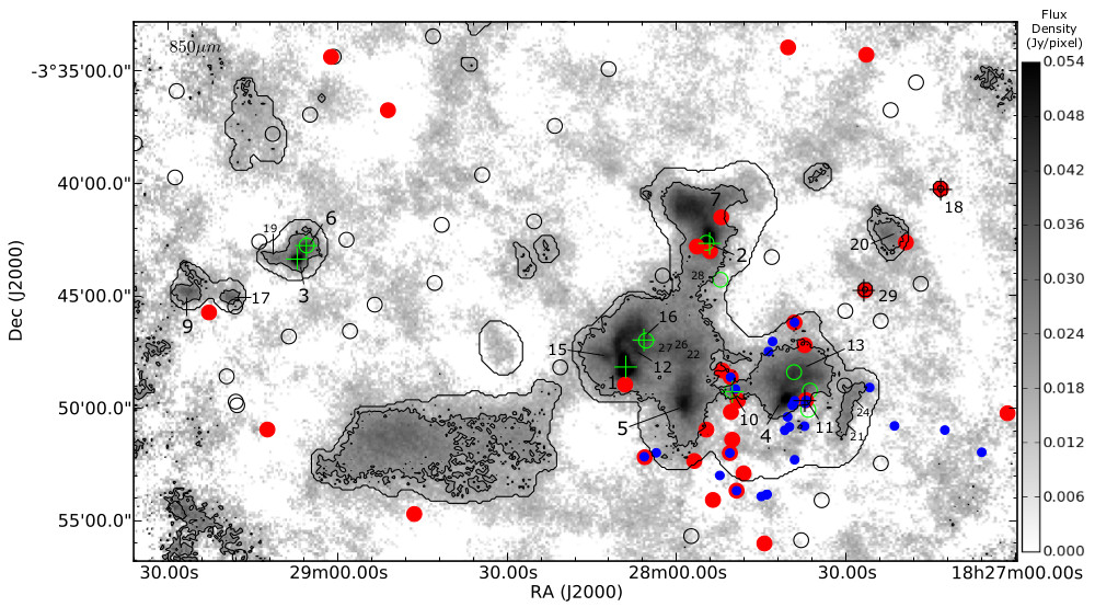
Figure 9: 850 $\micron$ greyscale map of Serpens MWC 297. Outer contours mark the data reduction mask (Figure 1) and inner contours the 3$\sigma$ detection level (0.0079 Jy/pixel). Circular markers indicate the location of YSOcs as catalogued by SGBSand crosses indicate the location of SCUBA-2 confirmed YSOs (Table 6). YSOcs are coded by evolutionary classification based on their spectral indices ($\alpha_{\mathrm{IR}}$) in the Spitzer case and by bolometric temperature, $T_{\mathrm{bol}}$, in the SCUBA-2 case (Table 6). Spitzer YSOcs are indicated by hollow black circles (Class III), solid red circles (Class II) and green hollow circles (Class 0/I). SCUBA-2 confirmed YSOs are indicated by black crosses (Class II) and green crosses (Class 0/I). Small, solid blue circles mark the location of Damiani et al. (2006) X-ray sources, typically associated with Class II and III objects.

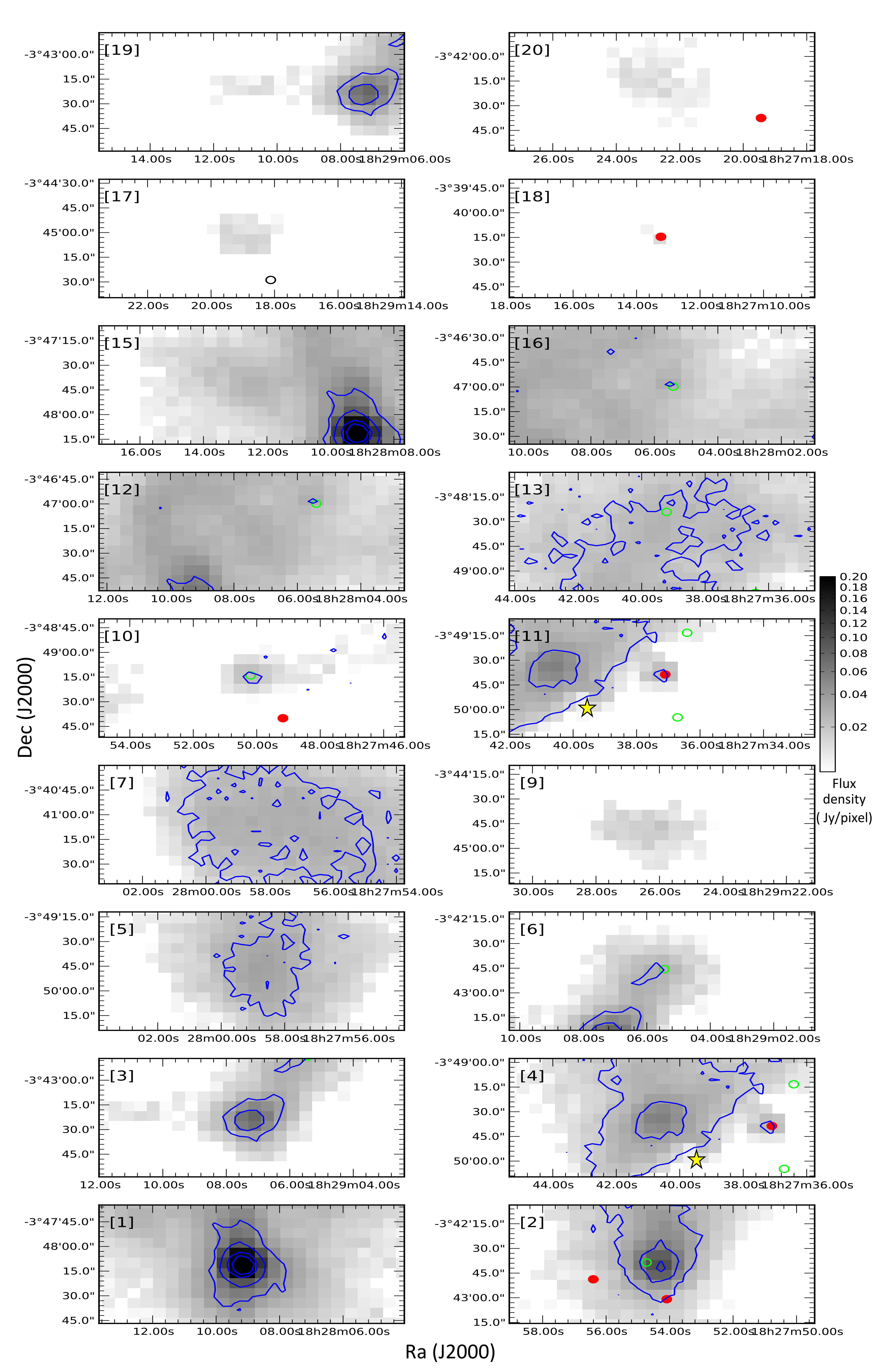
Figure 10: Comparison of flux emission from fellwalker objects at 450 $\micron$ (contours), 850 $\micron$ (greyscale) and the SGBS YSOcs (markers). Numbers in square brackets correspond to the objects in Table 3. Maps show contours of 450 $\micron$ submillimetre flux at 5, 10, 20 and 30 $\sigma$ ($\sigma$ = 0.016 Jy/pixel). Spitzer YSOcs are indicated by hollow black circles (Class III), solid red circles (Class II) and green hollow circles (Class 0/I). The star indicates the location of the star MWC 297.

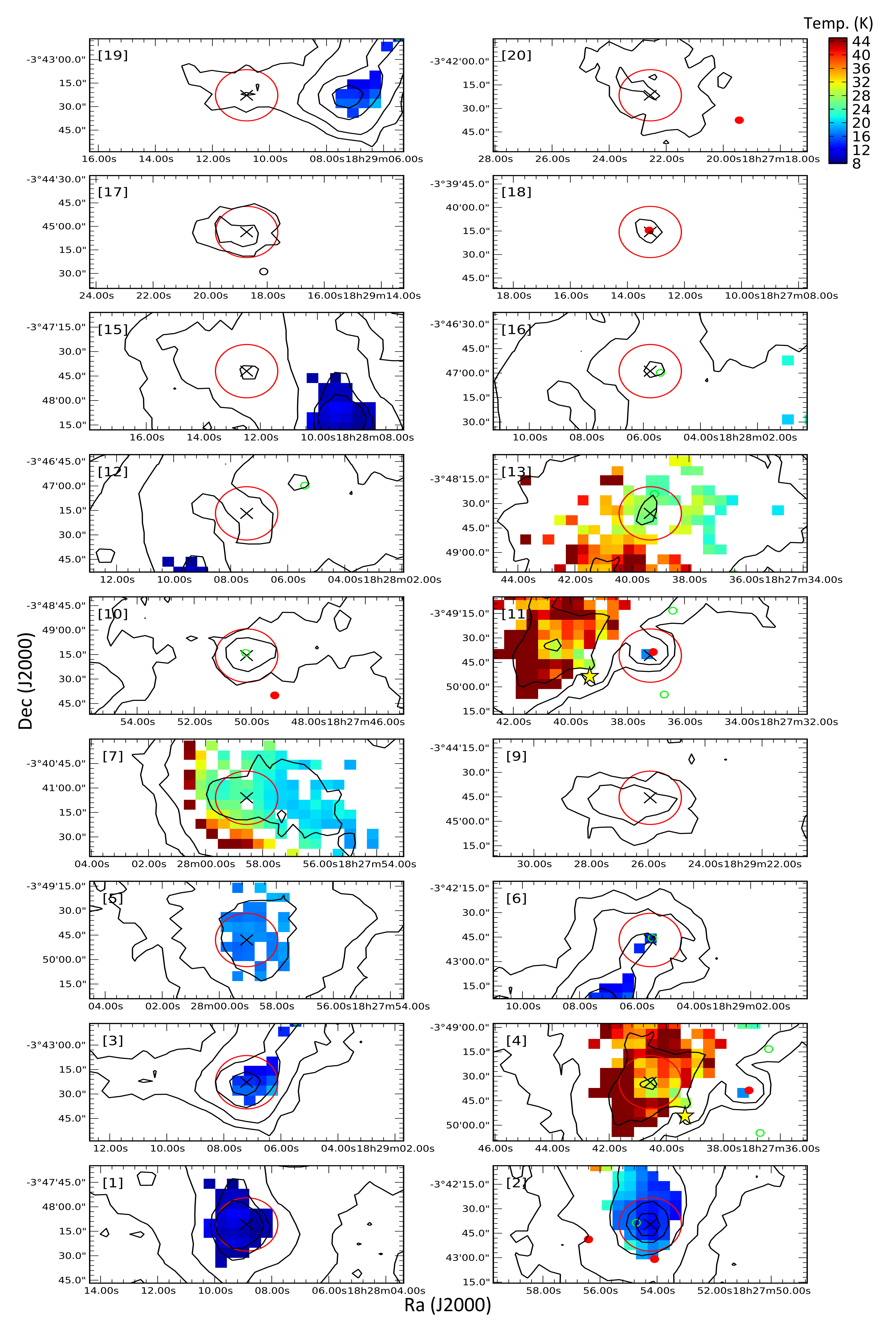
Figure 11: Submillimetre clumps in Serpens MWC 297 as identified by the fellwalker clump-finding algorithm. Numbers in square brackets correspond to the objects in Table 3. Maps show contours of 850 $\micron$ submillimetre flux at 5, 10, 20 and 30 $\sigma$ ($\sigma$ = 0.0022 Jy/pixel) up to the position of peak flux (black cross). The aperture from which SED flux density was calculated is plotted as the scale size of a protostellar core (0.05 pc). Temperature is shown where it is statistically significant and is used to calculate the masses shown in Table 6. Spitzer YSOcs are indicated by hollow black circles (Class III), solid red circles (Class II) and green hollow circles (Class 0/I). The star indicates the location of the star MWC 297.

5.2 SCUBA-2 YSO candidates

Table 6: Properties of YSO candidates in MWC 297.

IDa	$S_{\mathrm{450}}^{b}$	$S_{\mathrm{850}}^{b}$	$M_{\mathrm{850}}^{c}$	$T_{\mathrm{d}}^{d}$	$T_{\mathrm{bol}}^{e}$	$\alpha_{\mathrm{IR}}^{f}$	$L_{\mathrm{bol}}^{e}$	$L_{\mathrm{smm}}$/$L_{\mathrm{bol}}^{e}$	SGBS classg	Class
	(Jy)	(Jy)	(M${}_{\mathrm{\odot}})$	(K)	(K)		(L${}_{\mathrm{\odot}})$	per cent
S2-YSOc1	14.4	3.09	5.1(0.5)	10.3(0.5)	30(3)	1.65( 0.08)	1.1(0.1)	5.0(0.5)	‘Red’	0
S2-YSOc2	11.1	1.56	1.3(0.1)	15.6(0.8)	290(30)	0.56(0.05)	2.1(0.2)	1.9(0.2)	‘YSOc red’	I
S2-YSOc3	7.0	1.09	0.95(0.08)	14.8(0.7)	8(1)	1.4(0.7)	0.8(0.1)	3.0(0.3)	‘Flat’	0
S2-YSOc6	4.1	0.68	0.62(0.06)	14.2(0.7)	100(10)	0.30(0.05)	0.28(0.03)	5.2(0.5)	‘YSOc’	0/I
S2-YSOc10	4.5	0.37	0.31(0.03)	15.0(-)	190(20)	0.17(0.05)	0.82(0.08)	1.8(0.2)	‘YSOc star+dust’	I
S2-YSOc11	3.9	0.35	0.22(0.02)	17.6(0.9)	780(60)	-0.43(0.06)	3.3(0.2)	0.3(0.0)	‘YSOc’	II
S2-YSOc16	3.7	0.73	0.60(0.05)	15.0(-)	120(10)	0.9(0.3)	0.73(0.07)	1.9(0.2)	‘star F5V’	I
S2-YSOc18	0.1	0.11	0.09(0.02)	15.0(-)	820(50)	-0.17(0.05)	1.32(0.08)	0.1(0.0)	‘YSOc star+dust’	II
S2-YSOc29	4.0	0.36	0.30(0.03)	15.0(-)	860(50)	-0.49(0.05)	0.34(0.02)	0.1(0.0)	‘YSOc star+dust’	II
MWC	-	1.05	-	-	660(6)	-	422(4)	0.1(0.0)	‘2mass’	III
297

a) SCUBA-2 YSOcs (S2-YSOc) as identified by cross-referencing the SCUBA-2 clumps in Table 3 (Figure 11) with IR sources (Table 2).
b) Integrated fluxes of the YSOcs determined by fixed 40^′′ diameter aperture photometry. The uncertainty at 450 $\micron$ is 0.0165 Jy/pixel and at 850 $\micron$ is 0.0022 Jy/pixel. There is an additional systematic error in calibration of 10.6 per cent and 3.4 per cent at 450 $\micron$ and 850 $\micron$.
c) Mass as calculated with equation LABEL:eqn:mass. Errors in brackets are calculated from error in total flux, described in b., and error in mean temperature of 5 per cent. These results do not include the systematic error in distance (20 per cent) and opacity (factor of two).
d) Mean temperature as calculated from the temperature maps (Figure 3). Where no temperature data is available an arbitrary value of 15K(-) is assigned that is consistent with the literature.
e) YSOcs are classified using the $T_{\mathrm{bol}}$, $L_{\mathrm{bol}}$ and $L_{\mathrm{smm}}$/$L_{\mathrm{bol}}$ methods which are described in Section 5.4.
f) Values for spectral index are taken from the SGBS catalogue.
g) SGBS notation is described in Evans et al. (2009).

In this section we determine which members of the SCUBA-2 clump catalogue (Table 3) are starless and which host YSOs, as fellwalker is parameterised to identify both. The fellwalker algorithm is ideal for identifying larger scale, often irregular and extended clumps, but not effective for extracting the flux of individual YSOs, which are smaller. We extract a revised catalogue of YSOcs (Table 6) based on the position of the clumps listed in Table 3 and calculate the flux emission using aperture photometry with a fixed 40^′′diameter aperture.

Six clumps are found to contain SGBS YSOcs (Table 2) by cross-referencing the SCUBA-2 clumps in Table 3 (Figure 11) with IR sources (Table 2). Two further clumps (SMM 1 and 3) are found with little or no IR emission but are centrally condensed and have $M_{\mathrm{850}}/$$M_{\mathrm{J}}>1$ signifying they are gravitationally unstable and may be early protostellar (Class 0) YSOcs.

The following YSOcs-hosting clumps detected (SMM 1, 2, 3, 6, 10, 11, 16 and 18) are listed in Table 6 as SCUBA-2 YSO candidates (S2-YSOc). The remaining clumps listed in Table 3 do not contain YSOcs and are considered starless. SMM 4 and 7 are notable as they have relatively high masses (greater than 1 $M_{\mathrm{\odot}}$) but are not forming stars. SMM 5 has $M_{\mathrm{850}}/$$M_{\mathrm{J}}=1$ but there is no evidence for a 24 $\micron$ source there. It could be argued that this is a prestellar object on the cusp of becoming protostellar.

In addition to all those submillimetre objects identified by fellwalker, we also include one additional YSOc, S2-YSOc 29, as listed in Table 6 and YSOc11 in Table 2. This object fulfils the criterion of coincidence with a strong IR source in the Spitzer 24 $\micron$ MIPS data and a corresponding Class III identification in the SGBS YSOcs catalogue. S2-YSOc 29 registers a 5$\sigma$ detection with one pixel and resembles S2-YSOc 10 and 18 which are also believed to be an isolated, Class III PMS-stars with the remnants of an envelope/cold accretion disc contributing to their observed submillimetre flux.

Apertures were placed over the peak positions of the fellwalker clumps (Table 3) in addition to the Spitzer YSOcs positions and the integrated SCUBA-2 flux calculated with the intention to measure the flux from any dense, protostellar core associated with the SCUBA-2 clump peak and/or Spitzer YSOc. We follow Di Francesco et al. (2007), Sadavoy et al. (2010) and Rygl et al. (2013)’s definition of a core as a gravitationally bound, dense object, of diameter less than 0.05 pc and set apertures at this size (40^′′at 250 pc). Some larger scale emission is likely to be observed. However, through careful selection of aperture size we can assume that emission from the core dominates at this length scale.

Figures 9 and 10 show the locations of the SCUBA-2 YSOcs as well as those catalogued in the SGBS catalog. Figure 11 shows the relationship between the submillimetre peaks and the Spitzer YSOc position, with the SCUBA-2 fluxes for Spitzer YSOcs presented in Table 7. The mass of the SCUBA-2 YSOcs are calculated with Equation LABEL:eqn:mass, using a constant, mean temperature derived from our maps, and the results presented in Table 6.

A small number of Spitzer YSOcs inside the Herschel 500 $\micron$ data reduction mask are consistent with SCUBA-2 YSOcs with identical peak positions, for example in S2-YSOc 18 (Figure 11). In some cases, positions appear offset, for example S2-YSOc 2. This anomaly can be explained by virtue of the deeply embedded nature of the source and that Spitzer might be observing IR emission from an outflow cavity rather than the YSO itself.

YSOcs classified as 0/I by Spitzer should also have evidence of a SCUBA-2 peak at the same position. Those Spitzer detected protostars (YSOc16 and 38; Table 2) that lie outside of the 5$\sigma$ detection limit at 850 $\micron$ and have no obvious peak in emission are unlikely to be YSOcs and discarded as incorrectly classified objects.

A minority of cases detect greater than 5$\sigma$ flux but have no significant peak in emission, for example YSOc15 and 21. Examining these specific cases, both are classified as protostars and are deeply embedded within S2-YSOc13. Figure 3c shows how this region is near the centre of the reflection nebulae SH2-62 and therefore we interpret YSOc15 and 21 as IR emission from dust heated by the star MWC 297 and not real YSOcs. Many of the remaining Spitzer YSOcs detect low level, extended SCUBA-2 flux with no significant peak. No significant flux is detected for objects outside the mask.

Table 7: SCUBA-2 $40^{\prime\prime}$ aperture fluxes for the Spitzer YSOc listed in Table 2. A full version of this catalogue is available online.

ID	$S_{\mathrm{450}}$	$S_{\mathrm{850}}$	S2-YSOc ID
	Jy	Jy
YSOc1	$<0.72^{b}$	$<0.065^{b}$	-
YSOc2	$<0.72$	$0.115\pm 0.013$	S2-YSOc18
YSOc3	$<0.72^{b}$	$<0.065^{b}$	-
YSOc4	$<0.72^{b}$	$<0.065^{b}$	-
YSOc5	$<0.72^{b}$	$<0.065^{b}$	-
YSOc6	$<0.72^{b}$	$<0.065^{b}$	-
YSOc7	$<0.72^{b}$	$<0.065^{b}$	-
YSOc8	$<0.72^{b}$	$<0.065^{b}$	-
YSOc9	$<0.72^{b}$	$<0.065^{b}$	-
YSOc10	$<0.72^{b}$	$<0.065^{b}$	-
YSOc11	$<0.72$	$0.154\pm 0.013$	S2-YSOc29
YSOc12	$<0.72^{b}$	$<0.065^{b}$	-
YSOc13	$1.73\pm 0.14$a	$0.184\pm 0.013$a	-
YSOc14	$<0.72^{b}$	$<0.065^{b}$	-
YSOc15	$3.30\pm 0.14$a	$0.408\pm 0.013$a	-
YSOc16	$2.08\pm 0.14$a	$0.071\pm 0.013$a	-
YSOc17	$3.11\pm 0.14$	$0.362\pm 0.013$	S2-YSOc11
YSOc18	$2.10\pm 0.14$a	$0.263\pm 0.013$a	-
YSOc19	$<0.72^{b}$	$<0.065^{b}$	-
YSOc20	$1.11\pm 0.14$a	$0.112\pm 0.013$a	-
…	…	…	…

(a) Extended low level emission in aperture. No significant peak at YSOc position ($>3\sigma$).
(b) Outside data reduction mask. No significant flux detected in initial data reduction stage ($<5\sigma$).

5.3 Spectral Energy Distributions

SEDs are powerful tools for determining the properties of a star and we use these as an aid to classification through measurement of the spectral index across their IR wavebands, bolometric temperature and luminosity ratio (Evans et al., 2009).

SEDs are constructed from archival Two Micron All Sky Survey (2MASS) fluxes, Spitzer fluxes, and from SCUBA-2 fluxes. For the SCUBA-2 fluxes we conducted aperture photometry (as described in Section 5.2) at both 450 $\micron$ and 850 $\micron$ centred on the fellwalker clump peaks from Table 3. None of our sources overlapped sufficiently to make blended emission a problem.

Our primary sources are IRAC and MIPS data from the SGBS. Six out of nine objects are identified in the SGBS YSOc catalogue. We access the full SGBS source catalogue, which includes sources not classified as YSOcs, and find fluxes of each of the remaining three objects. S2-YSOc 1 and 3 are low luminosity objects that cannot be reliably classified as a YSOc by Spitzer and are therefore labelled ‘Red’ and ‘Flat’ following a description of their SEDs. Both objects have IRAC and MIPS fluxes that are many orders of magnitude less than their peers. S2-YSOc 16 has been classed as a F5V star. Following the work of Alonso-Albi et al. (2009) we bring together fluxes and present the SEDs in Figure 12 with specific cases of individual YSOs discussed in depth the following sections.

Many of the following methods directly use the SEDs constructed in this section to classify YSOs by examining how the flux of the object varies with wavelength.

5.4 YSO classification

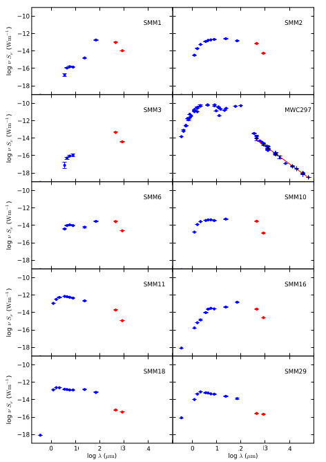
Figure 12: Spectral Energy Distributions for YSOcs associated with fellwalker clumps (Table 6). Blue points represent archive data sourced from Spitzer and 2MASS. Red points show new data provided by SCUBA-2 at 450 $\micron$ and 850 $\micron$ (note that the star MWC 297 was not identified by fellwalker after free-free contamination was accounted for). The straight line in MWC 297 describes free-free emission from an UCHII region and polar jet/wind with a spectral index $\alpha$=1.03.

Spectral index, $\alpha_{\mathrm{IR}}$, is a direct measurement of the gradient of the SED slope over an range of IR wavelengths (typically 2 to 24 $\micron$) and is expressed as

$$\alpha_{\mathrm{IR}}=\frac{d\log(\lambda S_{\lambda})}{d\log(\lambda)}.$$ (8)

Gutermuth et al. (2008) calculated $\alpha_{\mathrm{IR}}$ from the fluxes in the SGBS catalogue and we display these results in Table 6 and Table 2 for SGBS. As a classification tool for YSOs, $\alpha_{\mathrm{IR}}$ was developed by Lada & Wilking (1984) and Greene et al. (1994) and is summarised by Evans et al. (2009) who specify the boundaries between Class 0/I, FS, II and III as $\alpha_{\mathrm{IR}}$ = 0.3, -0.3 and -1.6.

$\alpha_{\mathrm{IR}}$ is one the most commonly used methods for the classification of protostars and consequently is one of the most criticised. Uncertainties on $\alpha_{\mathrm{IR}}$ typically vary between 10 and 20 per cent. However, measurements have been shown to be highly susceptible to disk geometry and source inclination (Robitaille et al., 2007) whilst extinction is known to cause $\alpha_{\mathrm{IR}}$ to appear larger. Furthermore, the development of $\alpha_{\mathrm{IR}}$ predates the identification of the Class 0 protostar (Chandler et al., 1990; Eiroa et al., 1994; André & Motte, 2000) and therefore does not distinguish between Class 0 and Class I when $\alpha_{\mathrm{IR}}$ is measurable (absence of $\alpha_{\mathrm{IR}}$ has been taken in this work to define a Class 0). Via the classification scheme outlined above, our sample contains four Class 0/I, two FS and three Class II sources. Saturation of Spitzer bands prevent measurement of $\alpha_{\mathrm{IR}}$ for MWC 297.

We calculate bolometric temperature, $T_{\mathrm{bol}}$, and luminosity, $L_{\mathrm{bol}}$, as alternative methods of classification of YSOs. We follow the numerical integration method of Myers & Ladd (1993) and Enoch et al. (2009) who calculated the discrete integral of the SED of an object for a given number of recorded fluxes. By adding SCUBA-2 data to that from the SGBS source catalogue, we extend the SEDs (Figure 12) for our YSOcs into the submillimetre spectrum and allow for a more complete integral from which we calculate $T_{\mathrm{bol}}$, the temperature of a black body with the same mean frequency of the observed SED, via

$$T_{\mathrm{bol}}=1.25\times 10^{-11}\bar{\nu}\,(\mathrm{K}\,\mathrm{Hz}^{-1}),$$ (9)

where $\bar{\nu}$ is the mean frequency of the whole spectrum,

$$\bar{\nu}=\frac{\int\nu S_{\nu}d\nu}{\int\nu d\nu}.$$ (10)

Classification separating boundaries for $T_{\mathrm{bol}}$ Class 0, I, II and III are 70, 350, 650 and 2800 K (Chen et al., 1995).

$T_{\mathrm{bol}}$ measurements for our sources are listed in Table 6. As this method uses more available data it could be considered a more reliable method of classification than $\alpha_{\mathrm{IR}}$ which only covers IRAC and MIPS bands 2 $\micron$ to 24 $\micron$. Furthermore $T_{\mathrm{bol}}$ provides a quantifiable method for separating Class I and Class 0. Similarly we calculate the ratio of submillimetre luminosity ($L_{\mathrm{smm}}$), defined as $\geq$ 350 $\micron$ by Bontemps et al. (1996), to $L_{\mathrm{bol}}$ in the method described by Myers et al. (1998) and Rygl et al. (2013), to classify YSOs:

$$L_{\mathrm{bol}}=4\pi d^{2}\int_{0}^{\infty}S_{\nu}d\nu,$$ (11)

and likewise for the submillimetre luminosity,

$$L_{\mathrm{smm}}=4\pi d^{2}\int_{0}^{350\micron}S_{\nu}d\nu.$$ (12)

This method was developed by André et al. (1993) who originally set the Class 0/I boundary at 0.5 per cent (subsequently used by Visser et al. (2002) and Young et al. (2003)). Maury et al. (2011) and Rygl et al. (2013) revise this upwards to 3 per cent and most recently Sadavoy et al. (2014) has used 1 per cent outlining the lack of consensus on this issue. We follow the work of Rygl et al. (2013) and classify objects with $L_{\mathrm{smm}}$/$L_{\mathrm{bol}}$ $\geq 3$ per cent as Class 0 protostars. Likewise, results for $L_{\mathrm{smm}}$/$L_{\mathrm{bol}}$ are listed in Table 6.

Our sample contains two Class 0 sources, four Class I and three Class II by $T_{\mathrm{bol}}$ and three Class 0 to six Class I, II & III sources by $L_{\mathrm{smm}}$/$L_{\mathrm{bol}}$ .

Uncertainties on $L_{\mathrm{bol}}$, $L_{\mathrm{smm}}$/$L_{\mathrm{bol}}$ and $T_{\mathrm{bol}}$ were calculated using a Monte Carlo method. A normal distribution of fluxes, with the mean on the measured flux at each wavelength for each YSO with a standard deviation equal to the original error on the measurements was produced. From each set of fluxes our classifications were calculated and the standard deviation on results listed in Table 6. The size of the uncertainties are consistent with Dunham et al. (2008). Dunham et al. (2008) and Enoch et al. (2009) both study the error on $L_{\mathrm{bol}}$ and $T_{\mathrm{bol}}$ and conclude incompleteness of the spectrum is a major source of systematic error in results of order approximately 31 per cent and 21 per cent (respectively) when compared to a complete spectrum. Enoch et al. (2009) find that the omission of the 70 $\micron$ flux is particularly critical when interpreting classification, leading to an overestimate of $L_{\mathrm{bol}}$ by 28 per cent and underestimate of $T_{\mathrm{bol}}$ by 18 per cent.

Figure 13 shows a direct comparison between the $\alpha_{\mathrm{IR}}$, $L_{\mathrm{smm}}$/$L_{\mathrm{bol}}$ and $T_{\mathrm{bol}}$ methods of classifying YSOs. As outlined above, each specialises in classification at different stages of evolution with $T_{\mathrm{bol}}$ arguably being the most effective for classifying protostars. Young et al. (2005) studied the merits of $T_{\mathrm{bol}}$ and $L_{\mathrm{smm}}$/$L_{\mathrm{bol}}$ and concluded that the latter is the more robust method for classifying Class 0 objects when compared to models of core collapse. However, it is also more sensitive to incompleteness of the submillimetre spectrum. With only two fluxes at wavelengths greater than 350 $\micron$ for the majority of the YSOs in MWC 297, we must consider the results from $L_{\mathrm{smm}}$/$L_{\mathrm{bol}}$ to be incomplete and therefore less reliable than $T_{\mathrm{bol}}$.

Out of the three objects classified as Class 0 by both $L_{\mathrm{smm}}$/$L_{\mathrm{bol}}$ and $T_{\mathrm{bol}}$ methods, only S2-YSOc 1 is consistent in both regimes. This object has a significantly positive value of $\alpha_{\mathrm{IR}}$ and so we classify this object as Class 0. The other two objects, S2-YSOc 3 and S2-YSOc 6, are forming in close proximity to each other but relatively isolated from the rest of the cloud. With a minimum separation of approximately 10,000 AU it seems likely that these objects formed together and therefore they are likely to be a similar class. S2-YSOc 3 has no noticeable IR flux at 24 $\micron$. However, the S2-YSOc 3 SED (Figure 12) shows Spitzer data consistent with emission from a heated region and so we conclude that the emission at 24 $\micron$ is sufficiently weak that it does not surpass the noise level and therefore does not appear in Figure 3c. Such low luminosity emission would be typical of Class 0 and therefore we label it as such. S2-YSOc 6 has a weak, if non-negligible, detection at 24 $\micron$ data. Therefore, we label it as Class 0/I. S2-YSOc 2 and 10 consistently fall into the Class I bracket by all three methods.

S2-YSOc 11, 18 and 29 all represent highly evolved and largely isolated cores that are consistently classified as Class II/III objects and have 24 $\micron$ detections in Figure 3c. Finally we discuss S2-YSOc16, an object labelled Class I by $T_{\mathrm{bol}}$ and by $\alpha_{\mathrm{IR}}$ and with a strong peak in the 24 $\micron$ data. Figure 11 shows how this object appears deep within an extended dust cloud. This scenario fits the definition of a Class I and the low mass of the object (0.60 $M_{\odot}$) when compared to the mass available in the neighbouring clumps (approximately 21 $M_{\odot}$) suggests that this object is early in its accretion life cycle.

6 Discussion

In this paper we use SCUBA-2 450 $\micron$ and 850 $\micron$ data and Spitzer data to investigate star formation in Serpens MWC 297 region. Taking the ratio of SCUBA-2 fluxes, we produce temperature maps of subregions of Serpens MWC 297 and calculate the properties of YSOs and clumps in the region.

Our work builds on analytical techniques developed for SCUBA data (Johnstone et al., 2000; Kirk et al., 2006; Sadavoy et al., 2010) to analyse SCUBA-2 data at the same wavelengths. SCUBA-2 represents a significant improvement over its predecessor as it has an array of 10,000 pixels, as opposed to 128. Practically this gives the instrument a much wider field of view and allows larger regions to be observed quicker and to greater depth. Restricted to SCUBA, larger regions of star formation, for example Orion (Nutter & Ward-Thompson, 2007) and Perseus (Hatchell et al., 2007), were prioritised over the low mass Serpens MWC 297 region.

The JCMT GBS extends the coverage of the local star-forming regions over those mapped by SCUBA. SCUBA-2 also offers much greater quality and quantity of 450 $\micron$ data, as a result of improved array technology and reduction techniques pioneered by Holland et al. (2006); Holland et al. (2013), Dempsey et al. (2013) and Chapin et al. (2013). Mitchell et al. (2001) is able to construct partial temperature maps from SCUBA 450 $\micron$ and 850 $\micron$ data but is limited to general statements about the region as a result of high noise estimates at 450 $\micron$. Reid & Wilson (2005) go further in their use of 450 $\micron$ data to analyse clump temperature but only obtain results for 54 per cent of the clumps they detect in 850 $\micron$. Calculated temperatures become increasingly unreliable at higher values to the extent they can only define a lower limit of 30 K for temperatures above this value.

The lower noise levels and wider coverage at 450 $\micron$ from SCUBA-2 offer improved quality and quantity to the extent that temperature maps can be constructed for many features in star-forming regions.

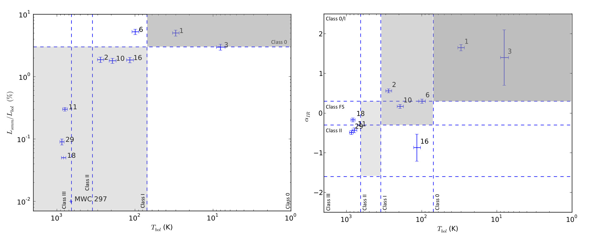
Figure 13: Bolometric temperature plotted against $L_{\mathrm{smm}}$/$L_{\mathrm{bol}}$ (left) and $\alpha_{\mathrm{IR}}$ (right) for the 10 YSOcs listed in Table 6. Dashed lines indicate the boundaries of classification of objects (greyed boxes indicating regions of class space where methods agree).

6.1 The state of star formation in Serpens MWC 297

Star formation is active and ongoing over a wide range of physical stages, from prestellar objects to Class III PMS-stars. We have detected 22 clumps in SCUBA-2 850 $\micron$ data using the clump-finding algorithm fellwalker (Table 3), from which we classify eight as YSOcs through consistency with 24 $\micron$ data and the SGBS YSOc catalogue. We include an additional Spitzer-detected YSOc (YSOc11) which was missed by fellwalker to provide us with a sample size of nine (Table 6), in addition to the 10 $M_{\odot}$ ZAMS star MWC 297. Seven (YSOc2, 11, 17, 32, 41, 47, 73) of these are found in the SGBS YSOc catalogues and two in the general SGBS source catalogue. Three Class 0, three Class I and three Class II sources are classified with SCUBA-2 data.

72 Class II/III and 10 Class 0/I sources are listed in the SGBS catalogue for the region. We do not expect to detect a high proportion of the Class II objects or any Class III objects with SCUBA-2. Figure 9 shows how few of these objects lie within the 3$\sigma$ detection level. We do expect to detect all Class 0 and most Class I objects with SCUBA-2 and therefore four (YSOc 15, 16, 21, 38) out of 10 Class 0/I sources listed in the SGBS catalogue that are not associated with SCUBA-2 peaks should be considered with scepticism. The remaining 16 objects identified by fellwalker are considered to be prestellar objects and diffuse clouds. From the SCUBA-2 catalogue every stage in star formation is represented up to stars on the main sequence. Given the assumed lifetime of each class, star formation has been active in this region for at least 3 Myr.

Star formation is observed at various stages in five large-scale clouds in the region which are composed of a number of fragmented clumps (Figure 7), the most evolved of which contain star forming cores. S2-YSOc 1 represents the most massive core we detect at 5.1$\pm$0.5 $M_{\mathrm{\odot}}$ and is the most prominent object in a larger cloud of mass 21$\pm$2 $M_{\mathrm{\odot}}$ - (see Figure 11). S2-YSOc 1 is the coolest YSO we have observed with mean temperature of 10.3$\pm$0.5 K and there is no evidence of heating in this region. If all the mass detected in S2-YSOc 1 accretes onto the core, allowing for a star-formation efficiency of 30 per cent (Evans et al., 2009), this object may go on to form an intermediate mass star similar to MWC 297.

A second cloud appears somewhat less fragmented with only two objects as opposed to four but also less massive with a peak core mass of 1.3$\pm$0.3 $M_{\mathrm{\odot}}$ and total cloud mass of 3.5 $M_{\mathrm{\odot}}$ (Figure 11 - S2-YSOc 2). Likewise a 30 per cent star-formation efficiency would limit the final mass to around 1 $M_{\mathrm{\odot}}$. S2-YSOc 3 and 6 (Figures 11) form a potentially loosely bound proto-binary composed of a Class 0 and Class I object with separation of 10,000 AU and masses 0.95$\pm$0.08 and 0.62$\pm$0.06 $M_{\mathrm{\odot}}$.

In addition to these deeply embedded, less evolved objects, a number of more evolved, isolated objects were observed. S2-YSOc 10, 18 and 29 are detached from the larger clouds and are much less luminous than the younger objects (Figure 11). At these stages, PMS-stars are dominated by disks rather than envelopes and we calculate masses of 0.31$\pm$0.03 $M_{\mathrm{\odot}}$, 0.09$\pm$0.02 $M_{\mathrm{\odot}}$ and 0.30$\pm$0.03 $M_{\mathrm{\odot}}$ for these objects. The protostar to PMS ratios suggest that these objects may have been formed in a dense region and later ejected or that the associated molecular cloud was larger in the past. Typical core migration speeds of 1 pc per Myr are consistent with the size of the observed region (30^′ diameter) and birth of these objects in one of the large clouds, most likely that associated with the star MWC 297 as it is the most evolved. S2-YSOc 11 and 16 are likely transition cores between Class I and II stages (Figure 11).

The remaining objects are not considered to be star-forming. The most massive of these are SMM 5 and 7 at 3.5$\pm$0.3 and 3.1$\pm$0.2 $M_{\mathrm{\odot}}$ (see Figure 11). We calculate free fall timescales of 2.1 and 1.8 Myrs for these objects. These are significantly larger than the typical protostellar timescale of 0.5 Myr are therefore unlikely to form stars without accreting mass or cooling further. The mean temperature of starless clumps is over twice that of star-forming cores (32$\pm$4 K to 15$\pm$2 K). Our observed core temperature is consistent with the assumption made in Section 4.2 and used by Johnstone et al. (2000) and Kirk et al. (2006). The remaining objects all have masses less than 1 $M_{\mathrm{\odot}}$ and are too diffuse to produce reliable temperature data. If these objects go onto to form stars, they are unlikely to form anything more massive than a brown dwarf.

A global analysis of the region reveals that, of a total cloud mass of 40 $M_{\mathrm{\odot}}$, only 12.5 $M_{\mathrm{\odot}}$ is not currently associated with ongoing star formation. Assuming a mean YSO mass of 0.5 $M_{\mathrm{\odot}}$ based of IMF observations (Chabrier, 2005; Evans et al., 2009), and given a mass of MWC 297 of 10 $M_{\odot}$ (Drew et al., 1997), we conclude that the total stellar (Class II or higher) mass of the region is 46 $M_{\odot}$. To date, approximately 85 per cent of the original cloud mass has gone into forming stars. From this we conclude that once this current generation of stars are formed, there is unlikely to be any further massive star formation without further mass accreting from the diffuse ISM and as a result we envisage a large distribution of low mass objects with the massive MWC 297 system dominating the region.

6.2 What does SCUBA-2 tell us about the star MWC 297?

The B1.5Ve star MWC 297 is a well known object. We comment on its relevant features and refer the reader to Sandell et al. (2011) for a comprehensive review the star’s properties.

MWC 297 is considered to be physically associated with the YSOcs within a 1^′ radius identified in SGBS and the additional YSO catalogues identified in Table 4 and displayed in Figure 9. MWC 297, objects 2MASS J18273854-0350108 (undetected in SCUBA-2) and 2MASS J18273670-0350047 (detected as S2-YSOc 11 in SCUBA-2) were found to have a mean group velocity of 0.01^′′per year (Roeser et al., 2008; Zacharias et al., 2012, 2013) providing evidence they were formed from same cloud. Further evidence in 24 $\micron$ data shown in Figure 3c shows how emission from warm dust heated by MWC 297, associated with SH2-62, is consistent with the location of dust clouds in the SCUBA-2 data. The angular distance between MWC 297 and the nearest clump (SMM 4) detected in SCUBA-2 amounts to a minimum physical separation of 5,000 AU, approximately half the size of our definition of a core (0.05 pc, Rygl et al. 2013).

We determine that free-free emission from an UCHII region and polar jets/winds associated with MWC 297 contaminates the 450 $\micron$ and 850 $\micron$ data (Skinner et al., 1993). The nature of the free-free emission from the outflow has been debated by various authors. Malbet et al. (2007) and Manoj et al. (2007) argue for ionised stellar winds that dominate at higher latitudes, whereas Skinner et al. (1993) and Sandell et al. (2011) provide evidence for an additional source of free-free emission in the form of highly collimated polar jets. Jets are typically associated with less evolved objects where luminosity is dominated by accretion processes whereas MWC 297 is considered to be a Class III / ZAMS star where the majority of the disk has fallen onto the star or been dissipated by winds. X-ray flares are thought to be a signature of episodic accretion and Damiani et al. (2006) detect a number of X-rays flares from the Serpens MWC 297 region but find that only 5.5 per cent of total flaring is directly associated with MWC 297, suggesting that accretion onto it is minimal. The majority of X-ray emission is associated with additional YSOs and the companion of MWC 297, OSCA, an A2V star identified by Habart et al. (2003) and Vink et al. (2005) at a separation of 850 AU.

Figure 6 and Figure 5 show that free-free emission due to an UCHII region and polar winds/jets is responsible for the majority of flux from the star MWC 297. Original peak fluxes of 188$\pm$16 mJy and 86$\pm$22 mJy are reduced to 51$\pm$11 mJy and 15$\pm$4 mJy at 450 $\micron$ and 850 $\micron$ respectively. The 5$\sigma$ level of 82 mJy and 11 mJy means that flux is too uncertain to be detected at 450$\micron$ and therefore it is not possible to calculate reliable temperatures of the residual circumstellar envelope/disk around the star. The assumption of point-like free-free emission may add further uncertainty to the residual flux.

Previous observations have interpreted a submillimetre source consistent with the location of MWC 297 as an accretion disk or circumstellar envelope (Di Francesco et al., 1994; Drew et al., 1997; Di Francesco et al., 1998). We believe that these observations can now be explained as free-free emission. Manoj et al. (2007) constrain the disk radius with radio observations to 80 AU and calculate a disk mass of M = 0.07 $M_{\mathrm{\odot}}$. These results are supported by Alonso-Albi et al. (2009) who conclude that this ‘exceptionally low’ disk mass is partly due to photoionisation by an UCHII region. Further work by Alonso-Albi et al. (2009) argues for the presence of a cold circumstellar envelope. Free-free does not account for emission at 70 $\micron$ and 100 $\micron$ as shown in the SED for MWC 297 (Figure 12) due to the exponential cutoff of the free-free power law as emission becomes optically thick at shorter wavelengths.

Our results do not rule out the presence of a disk or residual envelope following subtraction of the free-free emission, but they do confirm that any residual disk is low mass, though with a high degree of uncertainty as the submillimetre flux observed at the position of MWC 297 likely contains a component from the clump SMM 4 whichs overlaps this location. Temperature information about MWC 297 is also limited by the diminished size of the residual emission. We note that throughout this paper we have assumed a constant value of $\beta$ = 1.8. We have argued this a fair assumption for the ISM and extended envelope but this does not hold for the local environment of the protostar where the value of $\beta$ is known to be lower, leading to higher dust temperatures (see Figure 2).

Based on these observations we suggest the following arrangement whereby we are observing both the B star, MWC 297, and the companion A star, OSCA. MWC 297 has evolved further to the extent that it is producing the UCHII region observed. We find it unlikely that such a system could still be accreting matter on a large scale, or that the magnetic fields required to produce collimated jets could survive the UCHII region, and therefore we associate the jet emission observed by Skinner et al. (1993) to OSCA, an object that may be less evolved and more likely to still be in the accreting phase. Further evidence for active accretion onto OSCA has been provided by Damiani et al. (2006) who found substantial X-ray flaring from the object. A more massive disk structure would likely exist around the lower mass, and therefore less evolved, OSCA than MWC 297 and therefore this is likely the source of any residual SCUBA-2 flux and Spitzer MIPS flux observed in the combined SED. The separation at 850 AU is too small to resolve the two objects with the JCMT beam.

6.3 Is there evidence for radiative feedback in Serpens MWC 297?

The star MWC 297 is directly associated with the star-forming clumps identified in the SCUBA-2 data and the B star is directly heating those objects, none more so than SMM 4 where our result suggests that MWC 297 is directly influencing its evolution. A mean temperature of 46$\pm$2 K for SMM 4 was calculated, almost a factor of three times higher than the typical clump temperature of 15 K. The standard deviation of pixels of this clump is high at 11 K. The clump is warmest around the exterior with temperatures peaking above 55 K (potentially contributed to by edge effects) but it appears to have a cooler centre of 29 K (Figure 11). This is warmer than the mean temperature (18 K) of all the other clumps (discounting SMM 22 on account of its small size) detected by fellwalker. Heating of this object is not internal and the ISRF is not sufficient to produce such high temperatures. Only MWC 297 can provide sufficient external heating.

SMM 4 has a dust mass of 0.91$\pm$0.05 $M_{\mathrm{\odot}}$ but is the fourth most luminous clump in the region with a well defined, centrally condensed core. Raised temperatures mean that the object is gravitationally stable with a $M_{\mathrm{850}}/$$M_{\mathrm{J}}$ ratio of 0.12. From these results we conclude that, in the past, SMM 4 may have begun collapse on a similar timescale to MWC 297; however upon the B star producing sufficient radiation, MWC 297 has directly heated the larger part of the neighbouring clump to the extent that gravitational collapse is no longer possible, in effect suppressing, or even halting, the star formation process. Whether or not the low mass of SMM 4 or the power of MWC 297 is the limiting factor in this process remains unknown.

The majority of the other clumps detected show little or no external heating and no objects show evidence of internal heating. Table 3 outlines a range of mean clump dust temperatures, between 10 and 46 K, across the region. This is wider than the range of 12 to 20 K assumed by Motte et al. (1998) for Ophiuchus. Examining the mean temperatures of the Class 0 objects we find values of 12.6$\pm$0.9 K, below the assumed 15 K used by Johnstone et al. (2000) and Kirk et al. (2006) but within the range of Motte et al. (1998). Of the six Class 0/I objects, two (S2-YSOc 2 and 10) lie within the nebulosity whereas the remainder lie in regions with little significant emission from large scale heated dust as shown in Figure 11. None of the YSOcs show significant heating. However, use of a constant $\beta$ may not hold towards the centre of a protostar and our use of $\beta$ = 1.8 specifically for large structures maybe be systematically underestimating temperatures in these regions.

Starless object SMM 7 shows heating (Figure 11) along its eastern edge which is not consistent with the 24 $\micron$ emission. We suspect we are observing the ‘edge effect’ artefact produced in the map making process and this consequently increases temperature to 25$\pm$2 K. Conversely SMM 5 shows evidence of heated gas along its western edge in 24 $\micron$ emission (Figure 3c) but is relatively cool and homogenous in Figure 11 with a mean temperature of 18.2$\pm$0.9 K. Prohibitively high noise in the 450 $\micron$ data prevent wider examination of this feature.

7 Conclusion

We observed Serpens MWC 297 region with SCUBA-2 at 450 $\micron$ and 850 $\micron$ as part of the JCMT Gould Belt Survey of nearby star-forming regions. The observations covers a 30^′ diameter circular region centred on RA(J2000) = $18^{h}$ $28^{m}$ $13{\aas@@fstack{\prime\prime}}8$, Dec. (J2000) = $-03^{\circ}$ $44^{\prime}$ 1.7^′′ including the B1.5Ve Herbig Be star MWC 297 and a collection of local dense clouds. We use the clump-finding algorithm fellwalker to identity submillimetre clumps in the data and compare our catalogue to YSOc catalogues produced by the Spitzer Gould Belt Survey (SGBS), and to Spitzer 24 $\micron$ data of the region. The latter shows heating of surrounding clouds associated with the star MWC 297 and the optical nebula SH2-62, providing evidence that the two are physically located in space.

We account for sources of submillimetre contamination, finding an insignificant CO contamination estimated at 13 per cent but a significant amount from free-free emission as the result of an ultra-compact HII region and polar winds/jets associated with the star MWC 297. We use the ratio of 450 $\micron$ and 850 $\micron$ to build maps of dust temperature for Serpens MWC 297 with the aim of investigating evidence for radiative heating in the region. To do this we employed a method whereby each dataset is convolved with both the primary and secondary beam components of the JCMT beam at the other wavelength to achieve like resolution of 19.9^′′ before calculating the flux ratio and consequently temperature.

Our key results are:

1. Our temperature method uses both the primary and secondary components of the JCMT beam as this better reflects the shape of the real beam. The two component model decreases temperatures between 5 and 9 per cent in the warmest and coolest regions respectively.

2. We detect 22 clumps. By cross referencing this list with Spitzer YSOcs and a comparison of mass to Jeans mass as a test of gravitational stability, we identify nine YSOcs

3. We calculated masses based on calculated temperatures (as opposed to an assumed value) across the whole region. Clump masses range between 0.02-19 M$\odot$ and core masses range between 0.09-5.1 M$\odot$. Starless clumps are consistently warmer than star forming cores with mean temperatures of 32$\pm$4 K compared to 15$\pm$2 K.

4. We classify the YSOs using $T_{\mathrm{bol}}$ and $L_{\mathrm{smm}}$/$L_{\mathrm{bol}}$ as two Class 0, one Class 0/I, three Class I and three Class II sources. 30 per cent of Class 0/I objects and 8 per cent of Class II objects catalogued in SGBS were also detected by SCUBA-2. No Class III objects were detected by SCUBA-2. SCUBA-2 detected two potential Class 0 and one Class I/II YSOcs that were not included in the SGBS YSOc catalogue.

5. We modelled free-free emission from MWC 297 as a point-source with a spectral index of $\alpha=1.03\pm 0.02$. This contamination accounted for 73 per cent and 83 per cent of peak flux at 450 $\micron$ and 850 $\micron$ respectively. Residual peak fluxes were 51$\pm$10 mJy and 15$\pm$3 mJy respectively. The residual submillimetre emission for MWC 297 was insufficiently bright to be distinguishable from a larger clump (SMM 4) projected behind it on the sky.

6. We conclude that radiative heating from one generation of stars is directly influencing the formation of another, but we note that the effect is not large across the region. Our findings suggest that clump SMM 4 had begun collapsing before radiative heating from MWC 297 raised the temperatures to 46$\pm$2 K, to the extent that gravitational collapse is now suppressed or even halted.

Serpens MWC 297 region represents a low mass star-forming region with a limited number of YSOcs. We believe that in the future, this region will become dominated by the HII region associated with the star MWC 297. The expansion and shock front of this region will likely play an important role in the subsequent evolution of the cores and clumps we have detected. Further work will look at expanding these methods to produce temperature maps for larger regions within Serpens-Aquila, with a particular eye to possible free-free contamination where OB stars are observed to be forming.

The James Clerk Maxwell Telescope has historically been operated by the Joint Astronomy Centre on behalf of the Science and Technology Facilities Council of the United Kingdom, the National Research Council of Canada and the Netherlands Organisation for Scientific Research. Additional funds for the construction of SCUBA-2 were provided by the Canada Foundation for Innovation. The identification number for the program under which the SCUBA-2 data used in this paper is MJLSG33. This work was supported by a STFC studentship (Rumble) and the Exeter STFC consolidated grant (Hatchell). We would like to thank G$\ddot{o}$ran Sandell for the contribution of VLA data and the referee for their helpful feedback throughout the publishing process.

References

- Alonso-Albi et al. (2009) Alonso-Albi T., Fuente A., Bachiller R., Neri R., Planesas P., Testi L., Berné O., Joblin C., 2009, A&A, 497, 117
- André et al. (2010) André P., Men’shchikov A., Bontemps S., Könyves V., Motte F., Schneider N., Didelon P., Minier V., Saraceno P., Ward-Thompson D., 2010, A&A, 518, L102
- André & Motte (2000) André P., Motte F., 2000, in Favata F., Kaas A., Wilson A., eds, Star Formation from the Small to the Large Scale Vol. 445 of ESA Special Publication, FIRST and the Earliest Stages of Star Formation. p. 219
- André et al. (1993) André P., Ward-Thompson D., Barsony M., 1993, ApJ, 406, 122
- Arce & Goodman (1999) Arce H. G., Goodman A. A., 1999, ApJ, 517, 264
- Bate (2009) Bate M. R., 2009, MNRAS, 392, 1363
- Bergner et al. (1988) Bergner Y. K., Kozlov V. P., Krivtsov A. A., Miroshnichenko A. S., Yudin R. V., Yutanov N. Y., Dzhakusheva K. G., Kuratov K. S., Mukanov B. D., 1988, Astrofizika, 28, 529
- Berrilli et al. (1992) Berrilli F., Corciulo G., Ingrosso G., Lorenzetti D., Nisini B., Strafella F., 1992, ApJ, 398, 254
- Berry et al. (2007) Berry D. S., Reinhold K., Jenness T., Economou F., 2007, in Shaw R. A., Hill F., Bell D. J., eds, Astronomical Data Analysis Software and Systems XVI Vol. 376 of Astronomical Society of the Pacific Conference Series, CUPID: A Clump Identification and Analysis Package. p. 425
- Berry et al. (2013) Berry D. S., Reinhold K., Jenness T., Economou F., , 2013, CUPID: Clump Identification and Analysis Package
- Bonnor (1956) Bonnor W. B., 1956, MNRAS, 116, 351
- Bontemps et al. (2010) Bontemps S., André P., Könyves V., Men’shchikov A., Schneider N., Maury A., Peretto N., Arzoumanian D., Attard M., Motte F., Minier V., 2010, A&A, 518, L85
- Bontemps et al. (1996) Bontemps S., Andre P., Terebey S., Cabrit S., 1996, A&A, 311, 858
- Calvet & Gullbring (1998) Calvet N., Gullbring E., 1998, ApJ, 509, 802
- Canto et al. (1984) Canto J., Rodriguez L. F., Calvet N., Levreault R. M., 1984, ApJ, 282, 631
- Chabrier (2005) Chabrier G., 2005, in Corbelli E., Palla F., Zinnecker H., eds, The Initial Mass Function 50 Years Later Vol. 327 of Astrophysics and Space Science Library, The Initial Mass Function: from Salpeter 1955 to 2005. p. 41
- Chandler et al. (1990) Chandler C. J., Gear W. K., Sandell G., Hayashi S., Duncan W. D., Griffin M. J., Hazella S., 1990, MNRAS, 243, 330
- Chapin et al. (2013) Chapin E. L., Berry D. S., Gibb A. G., Jenness T., Scott D., Tilanus R. P. J., Economou F., Holland W. S., 2013, MNRAS, 430, 2545
- Chen et al. (1995) Chen H., Myers P. C., Ladd E. F., Wood D. O. S., 1995, ApJ, 445, 377
- Connelley & Greene (2010) Connelley M. S., Greene T. P., 2010, AJ, 140, 1214
- Curtis et al. (2010) Curtis E. I., Richer J. S., Swift J. J., Williams J. P., 2010, MNRAS, 408, 1516
- Damiani et al. (2006) Damiani F., Micela G., Sciortino S., 2006, A&A, 447, 1041
- Deharveng et al. (2012) Deharveng L., Zavagno A., Anderson L. D., Motte F., Abergel A., André P., Bontemps S., Leleu G., Roussel H., Russeil D., 2012, A&A, 546, A74
- Dempsey et al. (2013) Dempsey J. T., Friberg P., Jenness T., Tilanus R. P. J., Thomas H. S., Holland W. S., Bintley D., Berry D. S., Chapin E. L., Chrysostomou A., Davis G. R., Gibb A. G., Parsons H., Robson E. I., 2013, MNRAS, 430, 2534
- Di Francesco et al. (2007) Di Francesco J., Evans II N. J., Caselli P., Myers P. C., Shirley Y., Aikawa Y., Tafalla M., 2007, Protostars and Planets V, pp 17–32
- Di Francesco et al. (1994) Di Francesco J., Evans II N. J., Harvey P. M., Mundy L. G., Butner H. M., 1994, ApJ, 432, 710
- Di Francesco et al. (1998) Di Francesco J., Evans II N. J., Harvey P. M., Mundy L. G., Butner H. M., 1998, ApJ, 509, 324
- Drabek et al. (2012) Drabek E., Hatchell J., Friberg P., Richer J., Graves S., Buckle J. V., Nutter D., Johnstone D., Di Francesco J., 2012, MNRAS, 426, 23
- Drew et al. (1997) Drew J. E., Busfield G., Hoare M. G., Murdoch K. A., Nixon C. A., Oudmaijer R. D., 1997, MNRAS, 286, 538
- Dunham et al. (2008) Dunham M. M., Crapsi A., Evans II N. J., Bourke T. L., Huard T. L., Myers P. C., Kauffmann J., 2008, ApJS, 179, 249
- Dzib et al. (2010) Dzib S., Loinard L., Mioduszewski A. J., Boden A. F., Rodríguez L. F., Torres R. M., 2010, ApJ, 718, 610
- Dzib et al. (2011) Dzib S., Loinard L., Mioduszewski A. J., Boden A. F., Rodríguez L. F., Torres R. M., 2011, in Revista Mexicana de Astronomia y Astrofisica Conference Series Vol. 40 of Revista Mexicana de Astronomia y Astrofisica Conference Series, VLBA astrometry of the AeBe star EC 95 in Serpens. pp 231–232
- Ebert (1955) Ebert R., 1955, Zeitschrift fuer Astrophysik, 37, 217
- Eiroa et al. (1994) Eiroa C., Casali M. M., Miranda L. F., Ortiz E., 1994, A&A, 290, 599
- Eiroa et al. (2008) Eiroa C., Djupvik A. A., Casali M. M., 2008, in Reipurth B., ed., , Handbook of Star Forming Regions, Volume II. Monograph, p. 693
- Enoch et al. (2011) Enoch M. L., Corder S., Duchêne G., Bock D. C., Bolatto A. D., Culverhouse T. L., Kwon W., Lamb J. W., Leitch E. M., Marrone D. P., Muchovej S. J., Pérez L. M., Scott S. L., Teuben P. J., Wright M. C. H., Zauderer B. A., 2011, ApJS, 195, 21
- Enoch et al. (2009) Enoch M. L., Evans II N. J., Sargent A. I., Glenn J., 2009, ApJ, 692, 973
- Evans et al. (2003) Evans N. J. II., Allen L. E., Blake G. A., Boogert A. C. A., Bourke T., Harvey P. M., Kessler J. E., Koerner D. W., Lee C. W., Mundy L. G., Myers P. C., Padgett D. L., Pontoppidan K., Sargent A. I., Stapelfeldt K. R., van Dishoeck E. F., Young C. H., Young K. E., 2003, PASP, 115, 965
- Evans et al. (2009) Evans N. J. II., Dunham M. M., Jørgensen J. K., Enoch M. L., Merín B., van Dishoeck E. F., Alcalá J. M., Myers P. C., Stapelfeldt K. R., 2009, ApJS, 181, 321
- Evans et al. (2007) Evans N. J. II., Harvey P. M., Dunham M., Huard T., Mundy L., Lai S.-p., Chapman N., Brooke T., Enoch M., Stapelfeldt K., 2007, Technical report, Final Delivery of Data from the c2d Legacy Project: IRAC and MIPS. Spitzer Science Center, Pasadena, CA
- Fazio et al. (2004) Fazio G. G., Hora J. L., Allen L. E., Ashby M. L. N., Barmby P., Deutsch L. K., Huang J.-S., Kleiner S., 2004, ApJS, 154, 10
- Font et al. (2001) Font A. S., Mitchell G. F., Sandell G., 2001, ApJ, 555, 950
- Greene et al. (1994) Greene T. P., Wilking B. A., Andre P., Young E. T., Lada C. J., 1994, ApJ, 434, 614
- Gutermuth et al. (2008) Gutermuth R. A., Bourke T. L., Allen L. E., Myers P. C., Megeath S. T., Matthews B. C., Jørgensen J. K., Di Francesco J., Ward-Thompson D., Huard T. L., Brooke T. Y., Dunham M. M., Cieza L. A., Harvey P. M., Chapman N. L., 2008, ApJ, 673, L151
- Gutermuth et al. (2009) Gutermuth R. A., Megeath S. T., Myers P. C., Allen L. E., Pipher J. L., Fazio G. G., 2009, ApJS, 184, 18
- Habart et al. (2003) Habart E., Testi L., Natta A., Vanzi L., 2003, A&A, 400, 575
- Harvey et al. (2007) Harvey P., Merín B., Huard T. L., Rebull L. M., Chapman N., Evans II N. J., Myers P. C., 2007, ApJ, 663, 1149
- Harvey et al. (2008) Harvey P. M., Huard T. L., Jørgensen J. K., Gutermuth R. A., Mamajek E. E., Bourke T. L., Merín B., Cieza L., Brooke T., Chapman N., Alcalá J. M., Allen L. E., Evans II N. J., Di Francesco J., Kirk J. M., 2008, ApJ, 680, 495
- Hatchell et al. (2007) Hatchell J., Fuller G. A., Richer J. S., Harries T. J., Ladd E. F., 2007, A&A, 468, 1009
- Hatchell et al. (2005) Hatchell J., Richer J. S., Fuller G. A., Qualtrough C. J., Ladd E. F., Chandler C. J., 2005, A&A, 440, 151
- Hatchell et al. (2012) Hatchell J., Terebey S., Huard T., Mamajek E. E., Allen L., Bourke T. L., Dunham M. M., Gutermuth R., Harvey P. M., Jørgensen J. K., Merín B., Noriega-Crespo A., Peterson D. E., 2012, ApJ, 754, 104
- Hatchell et al. (2013) Hatchell J., Wilson T., Drabek E., Curtis E., Richer J., Nutter D., Di Francesco J., Ward-Thompson D., JCMT GBS Consortium 2013, MNRAS, 429, L10
- Hennebelle & Chabrier (2011) Hennebelle P., Chabrier G., 2011, ApJ, 743, L29
- Henning & Sablotny (1995) Henning T., Sablotny R. M., 1995, Advances in Space Research, 16, 17
- Herbig (1960) Herbig G. H., 1960, ApJS, 4, 337
- Hildebrand (1983) Hildebrand R. H., 1983, QJRAS, 24, 267
- Hillenbrand et al. (1992) Hillenbrand L. A., Strom S. E., Vrba F. J., Keene J., 1992, ApJ, 397, 613
- Holland et al. (2006) Holland W., MacIntosh M., Fairley A., Kelly D., Montgomery D., Gostick D., Atad-Ettedgui E., Ellis M., Robson I., Hollister M., Woodcraft A., 2006, in Society of Photo-Optical Instrumentation Engineers (SPIE) Conference Series Vol. 6275 of Society of Photo-Optical Instrumentation Engineers (SPIE) Conference Series, SCUBA-2: a 10,000-pixel submillimeter camera for the James Clerk Maxwell Telescope
- Holland et al. (2013) Holland W. S., Bintley D., Chapin E. L., Chrysostomou A., Davis G. R., Dempsey J. T., Duncan W. D., Fich M., Friberg P., Halpern M., Irwin K. D., Jenness T., Kelly B. D., MacIntosh M. J., Robson E. I., 2013, MNRAS, 430, 2513
- Huttemeister et al. (1993) Huttemeister S., Wilson T. L., Henkel C., Mauersberger R., 1993, A&A, 276, 445
- Jeans (1902) Jeans J. H., 1902, Royal Society of London Philosophical Transactions Series A, 199, 1
- Jenness et al. (2013) Jenness T., Chapin E. L., Berry D. S., Gibb A. G., Tilanus R. P. J., Balfour J., Tilanus V., Currie M. J., , 2013, SMURF: SubMillimeter User Reduction Facility
- Johnstone et al. (2000) Johnstone D., Wilson C. D., Moriarty-Schieven G., Joncas G., Smith G., Gregersen E., Fich M., 2000, ApJ, 545, 327
- Juvela et al. (2011) Juvela M., Ristorcelli I., Pelkonen V.-M., Marshall D. J., Montier L. A., Bernard J.-P., Paladini R., Lunttila T., 2011, A&A, 527, A111
- Kaas et al. (2004) Kaas A. A., Olofsson G., bontemps S., André P., Nordh L., Huldtgren M., Prusti T., Persi P., Delgado A. J., Motte F., Abergel A., 2004, A&A, 421, 623
- Kirk et al. (2006) Kirk H., Johnstone D., Di Francesco J., 2006, ApJ, 646, 1009
- Kirk et al. (2009) Kirk J. M., Ward-Thompson D., Di Francesco J., Bourke T. L., Evans N. J., Merín B., Allen L. E., Cieza L. A., Dunham M. M., Harvey P., Huard T., Jørgensen J. K., Miller J. F., Noriega-Crespo A., Peterson D., Ray T. P., Rebull L. M., 2009, ApJS, 185, 198
- Koenig et al. (2008) Koenig X. P., Allen L. E., Gutermuth R. A., Hora J. L., Brunt C. M., Muzerolle J., 2008, ApJ, 688, 1142
- Könyves et al. (2010) Könyves V., André P., Men’shchikov A., Schneider N., Arzoumanian D., Bontemps S., Attard M., Motte F., Didelon P., 2010, A&A, 518, L106
- Kraemer et al. (2003) Kraemer K. E., Jackson J. M., Kassis M., Deutsch L. K., Hora J. L., Simon R., Hoffmann W. F., Fazio G. G., Dayal A., Bania T. M., Clemens D. P., Heyer M. H., 2003, ApJ, 588, 918
- Lada & Wilking (1984) Lada C. J., Wilking B. A., 1984, ApJ, 287, 610
- Ladd et al. (1994) Ladd E. F., Myers P. C., Goodman A. A., 1994, ApJ, 433, 117
- Mairs et al. (2014) Mairs S., Johnstone D., Offner S. S. R., Schnee S., 2014, ApJ, 783, 60
- Malbet et al. (2007) Malbet F., Benisty M., de Wit W.-J., Kraus S., Meilland A., Millour F., Tatulli E., Berger J.-P., Chesneau O., Hofmann K.-H., Isella A., Natta A., Petrov R. G., Preibisch T., Stee P., Testi L., Weigelt G., Antonelli P., Beckmann U., 2007, A&A, 464, 43
- Mannings (1994) Mannings V., 1994, MNRAS, 271, 587
- Manoj et al. (2007) Manoj P., Ho P. T. P., Ohashi N., Zhang Q., Hasegawa T., Chen H.-R., Bhatt H. C., Ashok N. M., 2007, ApJ, 667, L187
- Mathis et al. (1983) Mathis J. S., Mezger P. G., Panagia N., 1983, A&A, 128, 212
- Maury et al. (2011) Maury A. J., André P., Men’shchikov A., Könyves V., Bontemps S., 2011, A&A, 535, A77
- Men’shchikov et al. (2010) Men’shchikov A., André P., Didelon P., Könyves V., Schneider N., Motte F., Bontemps S., Arzoumanian D., Attard M., Abergel A., Baluteau J.-P., Bernard J.-P., Cambrésy L., 2010, A&A, 518, L103
- Mitchell et al. (2001) Mitchell G. F., Johnstone D., Moriarty-Schieven G., Fich M., Tothill N. F. H., 2001, ApJ, 556, 215
- Motte et al. (1998) Motte F., Andre P., Neri R., 1998, A&A, 336, 150
- Myers et al. (1998) Myers P. C., Adams F. C., Chen H., Schaff E., 1998, ApJ, 492, 703
- Myers & Ladd (1993) Myers P. C., Ladd E. F., 1993, ApJ, 413, L47
- Nutter & Ward-Thompson (2007) Nutter D., Ward-Thompson D., 2007, MNRAS, 374, 1413
- Offner et al. (2009) Offner S. S. R., Klein R. I., McKee C. F., Krumholz M. R., 2009, ApJ, 703, 131
- Ossenkopf & Henning (1994) Ossenkopf V., Henning T., 1994, A&A, 291, 943
- Peterson et al. (2011) Peterson D. E., Caratti o Garatti A., Bourke T. L., Forbrich J., Gutermuth R. A., Jørgensen J. K., Allen L. E., Patten B. M., Dunham M. M., Harvey P. M., Merín B., Chapman N. L., Cieza L. A., Huard T. L., Knez C., Prager B., Evans N. J., 2011, ApJS, 194, 43
- Pilbratt et al. (2010) Pilbratt G. L., Riedinger J. R., Passvogel T., Crone G., Doyle D., Gageur U., Heras A. M., Jewell C., Metcalfe L., Ott S., Schmidt M., 2010, A&A, 518, L1
- Reid & Wilson (2005) Reid M. A., Wilson C. D., 2005, ApJ, 625, 891
- Rieke et al. (2004) Rieke G. H., Young E. T., Engelbracht C. W., Kelly D. M., Low F. J., Haller E. E., Beeman J. W., 2004, ApJS, 154, 25
- Robitaille et al. (2007) Robitaille T. P., Whitney B. A., Indebetouw R., Wood K., 2007, ApJS, 169, 328
- Roeser et al. (2008) Roeser S., Schilbach E., Schwan H., Kharchenko N. V., Piskunov A. E., Scholz R.-D., 2008, VizieR Online Data Catalog, 1312, 0
- Rosolowsky & Leroy (2006) Rosolowsky E., Leroy A., 2006, PASP, 118, 590
- Rosolowsky et al. (2008) Rosolowsky E. W., Pineda J. E., Foster J. B., Borkin M. A., Kauffmann J., Caselli P., Myers P. C., Goodman A. A., 2008, ApJS, 175, 509
- Rygl et al. (2013) Rygl K. L. J., Benedettini M., Schisano E., Elia D., Molinari S., Pezzuto S., André P., Bernard J. P., White G. J., Polychroni D., Bontemps S., Cox N. L. J., Di Francesco J., 2013, A&A, 549, L1
- Sadavoy et al. (2014) Sadavoy S. I., Di Francesco J., André P., Pezzuto S., Bernard J.-P., Maury A., Men’shchikov A., Motte F., 2014, ApJ, 787, L18
- Sadavoy et al. (2010) Sadavoy S. I., Di Francesco J., Bontemps S., Megeath S. T., Rebull L. M., Allgaier E., Carey S., Gutermuth R., Hora J., Huard T., McCabe C.-E., Muzerolle J., Noriega-Crespo A., Padgett D., Terebey S., 2010, ApJ, 710, 1247
- Sadavoy et al. (2013) Sadavoy S. I., Di Francesco J., Johnstone D., Currie M. J., Drabek E., Hatchell J., Nutter D., André P., Arzoumanian D., Benedettini M., 2013, ApJ, 767, 126
- Salji (2014) Salji C., 2014, in Protostars and Planets VI Posters Filament identification and characterisation in Gould Belt Clouds. p. 19
- Sandell et al. (2011) Sandell G., Weintraub D. A., Hamidouche M., 2011, ApJ, 727, 26
- Schnee et al. (2014) Schnee S., Mason B., Di Francesco J., Friesen R., Li D., Sadavoy S., Stanke T., 2014, ArXiv e-prints:
- Schnee et al. (2005) Schnee S. L., Ridge N. A., Goodman A. A., Li J. G., 2005, ApJ, 634, 442
- Sharpless (1959) Sharpless S., 1959, ApJS, 4, 257
- Shirley et al. (2002) Shirley Y. L., Evans II N. J., Rawlings J. M. C., 2002, ApJ, 575, 337
- Shirley et al. (2000) Shirley Y. L., Evans II N. J., Rawlings J. M. C., Gregersen E. M., 2000, ApJS, 131, 249
- Skinner et al. (1993) Skinner S. L., Brown A., Stewart R. T., 1993, ApJS, 87, 217
- Spezzi et al. (2011) Spezzi L., Vernazza P., Merín B., Allen L. E., Evans II N. J., Jørgensen J. K., Bourke T. L., Cieza L. A., Dunham M. M., Harvey P. M., Huard T. L., Peterson D., Tothill N. F. H., The Gould’s Belt Team 2011, ApJ, 730, 65
- Straižys et al. (2003) Straižys V., Černis K., Bartašiūtė S., 2003, A&A, 405, 585
- Stutz et al. (2010) Stutz A., Launhardt R., Linz H., Krause O., Henning T., Kainulainen J., Nielbock M., Steinacker J., André P., 2010, A&A, 518, L87
- Ubach et al. (2012) Ubach C., Maddison S. T., Wright C. M., Wilner D. J., Lommen D. J. P., Koribalski B., 2012, MNRAS, 425, 3137
- Vink et al. (2005) Vink J. S., O’Neill P. M., Els S. G., Drew J. E., 2005, A&A, 438, L21
- Visser et al. (2002) Visser A. E., Richer J. S., Chandler C. J., 2002, AJ, 124, 2756
- Ward-Thompson et al. (2007) Ward-Thompson D., Di Francesco J., Hatchell J., Hogerheijde M. R., Nutter D., Bastien P., Basu S., Bonnell I., Bowey J., Brunt C., Buckle J., 2007, PASP, 119, 855
- Watson (2010) Watson M., 2010, MSc thesis, University of Hertfordshire.
- Winston et al. (2007) Winston E., Megeath S. T., Wolk S. J., Muzerolle J., Gutermuth R., Hora J. L., Allen L. E., Spitzbart B., Myers P., Fazio G. G., 2007, ApJ, 669, 493
- Wood et al. (1994) Wood D. O. S., Myers P. C., Daugherty D. A., 1994, ApJS, 95, 457
- Young et al. (2003) Young C. H., Shirley Y. L., Evans II N. J., Rawlings J. M. C., 2003, ApJS, 145, 111
- Young et al. (2005) Young K. E., Harvey P. M., Brooke T. Y., Chapman N., Kauffmann J., Bertoldi F., Lai S.-P., Alcalá J., Bourke T. L., Spiesman W., Allen L. E., Blake G. A., Evans II N. J., 2005, ApJ, 628, 283
- Zacharias et al. (2012) Zacharias N., Finch C. T., Girard T. M., Henden A., Bartlett J. L., Monet D. G., Zacharias M. I., 2012, VizieR Online Data Catalog, 1322, 0
- Zacharias et al. (2013) Zacharias N., Finch C. T., Girard T. M., Henden A., Bartlett J. L., Monet D. G., Zacharias M. I., 2013, AJ, 145, 44
- Ziener & Eislöffel (1999) Ziener R., Eislöffel J., 1999, A&A, 347, 565