A Semi-Coherent Search for Weak Pulsations in Aql X–1

Abstract

Non pulsating neutron stars in low mass X-ray binaries largely outnumber those that show pulsations. The lack of detectable pulses represents a big open problem for two important reasons. The first is that the structure of the accretion flow in the region closest to the neutron star is not well understood and it is therefore unclear what is the mechanism that prevents the pulse formation. The second is that the detection of pulsations would immediately reveal the spin of the neutron star. Aql X–1 is a special source among low mass X-ray binaries because it has showed the unique property of pulsating for only ${\sim}$150 seconds out of a total observing time of more than 1.5 million seconds. However, the existing upper limits on the pulsed fraction leave open two alternatives. Either Aql X–1 has very weak pulses which have been undetected, or it has genuinely pulsed only for a tiny amount of the observed time. Understanding which of the two scenarios is the correct one is fundamental to increase our knowledge about the pulse formation process and understand the chances we have to detect weak pulses in other LMXBs. In this paper we perform a semi-coherent search on the entire X-ray data available for Aql X–1. We find no evidence for (new) weak pulsations with the most stringent upper limits being of the order of 0.3% in the 7–25 keV energy band.

1. Introduction

Some neutron stars in low mass X-ray binaries (LMXBs) have sufficiently strong magnetic fields to truncate the accretion disk and channel the plasma along the field lines. According to accretion theory (Ghosh et al., 1977; Ghosh & Lamb, 1978, 1979), the neutron star might be spun up in the process with the gas impacting on the surface and forming “hot spots” plus a shock right above it  (Basko & Sunyaev, 1976; Poutanen & Gierliński, 2003). Modulation of the thermal and comptonized radiation emerging in the process creates X-ray pulsations that reveal the spin period of the neutron star. Accreting millisecond X-ray pulsars (AMXPs) are neutron stars in low mass X-ray binaries (LMXBs) with spin period of less than ${\sim}10$ ms, which are powered via the process described above (Wijnands & van der Klis 1998, see Patruno & Watts 2012 for a recent review). However, among the ${\sim}150$ neutron stars in LMXBs, only ${\sim}20$ show pulsations and have been unambiguously identified as either AMXPs or as slow accreting pulsars (like Her X-1, GX 1+4, etc., see e.g., Table 1 in Patruno & Watts 2012 and Bildsten & Brown 1997). The large majority of neutron star LMXBs do not show accretion powered pulsations with typical upper limits on the pulsed fraction in the range of ${\sim}1$–$10\%$ rms (see for example Vaughan et al. 1994; Dib et al. 2005).

Many different possibilities have been proposed in the literature to explain the paucity of pulsators among LMXBs, the most popular including the onset of interchange instabilities that create a chaotic accretion flow stream (Kulkarni & Romanova, 2008), the smearing and scattering of pulsed emission (Brainerd & Lamb, 1987; Titarchuk et al., 2002), gravitational lensing (Wood et al., 1988; Özel, 2009), the nearly perfect alignment of the neutron star magnetic and spin axis (Ruderman, 1991; Lamb et al., 2009a) and the screening of the magnetosphere by the accreted matter (Bisnovatyi-Kogan & Komberg, 1974; Cumming et al., 2001). So far, however, the exact reason behind this behaviour remains not completely understood.

The discovery of the new phenomenon of intermittent pulsations(Galloway et al., 2007) might help to shed light on the mechanism that prevents most LMXBs from pulsating. Intermittent pulsations can be described as a sporadic appearance and disappearance of X-ray pulses (on variable timescales) during an outburst. HETE J1900.1–2455 was the first intermittent pulsar to be discovered (Kaaret et al., 2006; Galloway et al., 2007) and shows continuous pulsations for about 70 days since the beginning of its nine year long outburst (still ongoing at the moment of writing) with intermittent pulsations then appearing sporadically for the next 2.5 years (Galloway et al., 2007, 2008; Patruno, 2012). Pulsations were detected down to the 0.3% rms level (Galloway et al., 2008; Patruno, 2012), whereas in the proceeding years pulsations were not detected with the best upper limits on the fractional amplitude of 0.05% rms (95% confidence level, see Patruno 2012). During this time HETE J1900.1–2455 was completely indistinguishable from one of the many non-pulsating LMXBs (see e.g., Papitto et al. 2013). Gavriil et al. (2007) and Altamirano et al. (2008) discovered intermittent pulses in SAX J1748.9–2021 that appeared sporadically throughout two outbursts at unpredictable times. Finally, Casella et al. (2008) made the particularly surprising discovery of a single episode of pulsations in Aql X–1 (with 2–60 keV fractional semi-amplitude of approximately 2%), that lasted for only $\approx 150$ s over a total observing time of about 1.5 Ms. This discovery raised the question on whether all non pulsating LMXBs do show pulsations for very brief time intervals that could be easily missed, since the duty cycle of pulsations might be as short as in Aql X–1.

So far a big limitation in pulse searches has been the very large computational time required to analyze the huge amount of data available. The reason for this is that in most non-pulsating LMXBs the orbital parameters of the system are poorly known, leaving a parameter space too large to be searched. Indeed, simple techniques based on power spectral density estimation are very limited in terms of sensitivity if the pulse frequency drift due to Doppler motion in the binary is not corrected for. Casella et al. (2008) performed a complete RXTE archival data search for pulsations in Aql X–1, using standard Fourier transforms of 128s length. Such short data segments ensured that the spin frequency stays in one–two Fourier frequency bins during the observation, avoiding the spread of power in multiple bins due to orbital motion Doppler shifts. This search however is not optimal, since the signal can be accumulated only in very short data segments.

Another strategy employed is the so-called acceleration search method (Ransom et al., 2002). This strategy requires a sub-division of data into segments of no more than about 1/10 of the orbital period length so to have an approximately constant orbital acceleration over each specific data segment. The signal is then searched by summing the power in a certain amount of adjacent Fourier frequency bins where the signal has spread due to the acceleration of the neutron star.

The discovery of pulsations in all 17 known AMXPs (both intermittent and persistent) can be ascribed to the use of the first method whereas only the ultra-compact LMXB 4U 1820–30 has been thoroughly searched with the acceleration technique leading to upper limits of about 0.8% rms on the pulsed fraction (Dib et al., 2005).

In this paper we use a different approach to the problem. To account for the Doppler shift in the binary we use a so-called semi-coherent search strategy, initially developed to optimize computationally intensive gravitational wave searches (Messenger, 2011) but implemented and optimized in this work for deep pulse searches in X-ray binaries. The concept of the search is a generalization and extension of the acceleration search. Each segment of data is processed over a bank of signal model template waveforms. The waveforms approximate the binary Doppler modulation as a smooth phase evolution modelled by a Taylor expansion in frequency. The data products from each segment are represented by the Fourier power computed for each of these templates. This power is then summed over segments such that the excess power from all possible signals is tracked in frequency (and frequency derivatives) as the source moves through its binary orbit. This process affords an enhancement to the fractional amplitude sensitivity approximately proportional to the fourth root of the number of segments. Such a scheme is moderately computationally intensive and requires the use of many 1000s of CPU hours.

We applied the semi-coherent search scheme to all archival data of Aql X–1 recorded with high time resolution by the Rossi X-ray Timing Explorer (RXTE). Since previous pulse searches used short data segments of just 128 seconds, the sensitivity reached was only sufficient to detect pulse fractional semi-amplitudes of the order of 1% (see Casella et al. 2008) which is very close to the reported 2–60 keV pulsed fraction (semi–amplitude) of the single pulse episode ($1.9\pm 0.2\%$). Therefore it is plausible to expect that what we have observed so far is not really a single intermittent pulsation, which is indeed extremely problematic to explain from a theoretical point of view, but only the “tip of the iceberg” with a large amount of weak pulses lying below the detection sensitivity of previous pulse searches. We therefore will direct our efforts towards the search of weak (semi-amplitude of $\lesssim 1\%$) but continuous pulsations.

In Secs. 2 and 3 we discuss the RXTE data preparation and the Aql X–1 parameter space respectively. We then describe the data preprocessing in Sec. 4 and our semi-coherent detection statistic in Sec. 5. In Sec. 6 we describe how our search for pulsations from Aql X–1 was implemented and the corresponding results are described in Sec. 7. A discussion of our findings is given in Sec. 8 and we conclude with Sec. 9.

2. X-ray Observations and Data Preparation

RXTE has observed Aql X–1 for ${\sim}15$ years, collecting data of 20 outbursts and recording high time resolution data with the Proportional Counter Array (PCA; see Jahoda et al. 2006) for 18 of them. Each outburst lasts for a variable amount of time, from few days up to six months, with a recurrence time of ${\sim}1$ yr (see e.g., Campana et al. 2013 and their Table 1). We performed a complete archival search on all RXTE public data available collected between January 1997 and October 2010 (see Table 1).

Table 1RXTE observations of Aql X–1 from 1997 to 2010

Year	Index	Program IDs
1997 Jan	1	20098
1997 Aug	2	20091
1998 Feb	3	30072, 30073, 30188
1999 May	4	40033, 40047, 40048 40049, 40432
2000 Sep	5	50049
2001 Jun	6	60054
2002 Feb	7	60429, 70069
2003 Feb	8	70426, 80403
2004 Feb	9	80403, 90403, 90017
2005 Mar	10	91028, 91414
2005 Nov	11	91414
2006 Jul	12	92034
2007 May	13	92438, 92076
2007 Sep	14	93045
2008 May	15	93045, 93076
2009 Mar	16	94076
2009 Nov	17	94076, 94441
2010 Sep	18	95086, 95413

We used all pointed observations taken in GoodXenon or in Event 122$\mu\,s$ mode with time resolution of $2^{-20}$ s and $2^{-13}$ s, respectively. The GoodXenon data were rebinned to match the same time resolution of the Event data. We selected an energy band between 7 and 25 keV which is based on the maximization of the signal-to-noise ratio (S/N) of the single ${\sim}150$s pulse episode previously detected in this source. Indeed, as noticed by Casella et al. (2008), the pulsed fraction of Aql X–1 increases with energy, growing from less than 1-2% at low energies ($<5$ keV) to 10–20% in the highest energy band (10–30 keV).

To inspect for the presence of thermonuclear bursts we construct the 2–16 keV X-ray light curve with the PCA Standard 2 data (16 s time resolution). We refer to van Straaten et al. (2003) for further details on the light-curve generation. The start and end time of thermonuclear bursts are defined as the points where the count rate in the lightcurve is twice the pre-burst value. The high time resolution data are then barycentered at the best determined radio position of Aql X–1 (Tudose et al., 2013) and are filtered according to standard procedures: unstable pointings, thermonuclear bursts and passages through the South Atlantic anomaly are removed from the data. When an X-ray burst occurs, the data are split into two time-series, a pre-burst and a post-burst. The largest majority of final-product time series have a duration in the range 1–3 ks.

3. Aql X–1: Parameter Space

Aql X–1 has a relatively well constrained orbital and spin parameters. The orbital period has been determined from optical observations and constrained to be $18.9479\pm 0.0002$ hr (Chevalier & Ilovaisky, 1991, 1998). Welsh et al. (2000) reported a slightly shorter orbital period ($18.71\pm 0.06$ hr) which was considered consistent with the value reported by Chevalier & Ilovaisky (1998) due to unaccounted systematics. We choose to define a safe orbital period range with values between 18.5 and 19.2 hours. The orbital phase is considered unknown and we therefore consider the range 0 to 1 cycles as our search space.

The spin frequency is also known with good precision to be around 550 Hz thanks to burst oscillation measurements (Zhang et al., 1998) and the possible single accretion powered episode reported by Casella et al. (2008). In particular, Casella et al. (2008) reported a spin frequency of $550.273(1)$ Hz, which is, however, not corrected for the Doppler shift of the neutron star in the binary. To determine the effect of the Doppler shift we explored a broad range of projected semi-major axis values that span between 0.1 and 4.2 light-seconds. In this case the term “projected” indicates the true orbital semi-major axis projected along the line of sight of our observation. Combined with our orbital periods, this gives a range of possible pulse frequencies between 549.9 and 550.6 Hz. Finally, we assume zero orbital eccentricity, which is a good approximation for LMXBs. We note that as indicated in Fig. 3 of Messenger (2011) for our search and its corresponding parameters we are insensitive to eccentricity below $\lesssim 0.01$.

The complete physical Aql X–1 parameter space for this search is therefore 4 dimensional. We assume no a-priori correlations between our search parameters and hence our search space is equal to the Cartesian product of the intrinsic spin frequency $f$, the projected orbital semi-major axis $a$, the orbital period $P$ and the orbital phase $\psi$. This space is limited in each dimension by the ranges specified above and in Table 2.

Table 2The pulse frequency and orbital parameter space boundaries for the AQL X–1 search.

Parameter	Units	Min	Max
$f$	Hz	549.9	550.6
$a$	s	0.1	4.2
$P$	hr	18.5	19.2
$\psi$	rads	0	$2\pi$

4. Data preprocessing

The data is first divided into outbursts 1–18, and for each outburst the data is comprised of multiple contiguous time-series. Each time-series is initially processed with a time-domain high pass 10th order Butterworth filter with filter frequency $40$ Hz in order to remove any spurious low-frequency modulation. Each contiguous stretch of data is then further subdivided into segments of length $T=256$s. This choice is based on computational constraints and is further discussed in Sec. 7.1. These “segments” now containing gap-free time-series data are Fourier transformed according to

$$\tilde{x}_{k}=\sum_{j=0}^{N-1}x_{j}e^{-2\pi ijk/N}$$ (1)

where the time-series data $x_{j}$ represents the photon count in the $j$’th time bin and where the time index $j$ ranges from 0 to $N=T/\Delta t$ and $\Delta t=2^{-13}$s is the sampling time. Within the process of subdividing into segments, stretches of data of length $<T$ s or data left at the ends of time-series after division that were $<T$ s were discarded at the expense of losing $\approx 5.7\%$ of the total data. Since our search concerns a relatively narrow frequency band for the intrinsic spin frequency of the source, we also only retain Fourier frequency bins within the range 549–552 Hz.

5. The detection statistic

Considering a single segment of X–ray data, we model our binned timeseries $\bm{x}$ as Poisson distributed such that the likelihood function for a single segment of data is

$$p(\bm{x}|\bm{\Theta},I)=\prod_{j=0}^{N-1}\frac{r_{j}(\bm{\Theta})^{x_{j}}e^{-r_{j}(\bm{\Theta})}}{x_{j}!}$$ (2)

where $\bm{\Theta}$ is a vector of signal parameters (including our search parameters) that define our signal model given by

$$r_{j}(\bm{\Theta})=R\left(1+A\sin\left(\phi_{j}(\bm{\theta})+\beta\right)\right).$$ (3)

Here $R$ is the expected background counts per time bin, $A$ is the pulsed fraction of our signal, $\phi_{j}(\bm{\theta})$ is the time dependent phase of the signal and $\beta$ is a reference phase of the signal. The parameter vector $\bm{\theta}$ are our search parameters and a subset of the complete signal parameters $\bm{\Theta}$.

The null hypothesis assumes that no signal is present in the data and we can therefore define the null, or noise-only, model using Eq. 3 and setting $A=0$. The log-likelihood-ratio between our signal and noise-only models can be approximated as

$$\Lambda =\sum_{j=0}^{N-1}x_{j}\log\left(1+A\sin\left(\phi_{j}(\bm{\theta})+\beta\right)\right)$$

$$-RA\sin\left(\phi_{j}(\bm{\theta})+\beta\right)$$

$$\approx-\frac{1}{4}NRA^{2}+A\sum_{j=0}^{N}x_{j}\sin\left(\phi_{j}(\bm{\theta})+\beta\right)$$ (4)

where we have assumed that we are working in the weak signal regime and used the approximation $A\ll 1$.

The log-likelihood ratio can now be analytically maximized over the unknown amplitude and phase parameters $A$ and $\beta$ to give

$$2\hat{\Lambda}(\bm{\theta})=2\frac{|\tilde{x}(\bm{\theta})|^{2}}{NR}$$ (5)

where we define the phase model demodulated Fourier transform of the data as

$$\tilde{x}(\bm{\theta})=\sum_{j=0}^{N-1}x_{j}\exp\left(-i\phi_{j}(\bm{\theta})\right).$$ (6)

For a monochromatic phase model this expression is simply the discrete Fourier transform evaluated at a specific frequency (equivalent to Eq. 1). In general our phase model will deviate from monochromicity according to the binary motion of the source. This statistic is $\chi^{2}$ distributed with 2 degrees of freedom and a non-centrality parameter equal to the signal-to-noise ratio (SNR) of the signal within this segment. Assuming a set of signal parameters evaluated at an offset parameter space location $\bm{\theta}+\bm{\Delta\theta}$, the expectation value of the single segment detection statistic is

$$\text{E}\left[2\hat{\Lambda}(\bm{\theta},\bm{\Delta\theta})\right]=2+\rho^{2}(\bm{\theta},\bm{0})\left|\frac{1}{N}\sum\limits_{j=0}^{N-1}e^{-i\Delta\phi_{j}(\bm{\theta},\bm{\Delta\theta})}\right|^{2}.$$ (7)

We have defined the optimal coherent SNR as the total noise-free signal power weighted by the noise such that

$$\rho^{2}(\bm{\theta},\bm{0})=\frac{4}{S_{\text{n}}}\int|\tilde{r}(\bm{\theta})|^{2}df=\frac{NRA^{2}}{2}$$ (8)

where for all non-zero frequencies $S_{\text{n}}{=}2\Delta tR$ is the single-sided noise spectral density. Here we see the standard result that the SNR is proportional to the signal amplitude and to the square-root of the observation time since $T\propto N$.

As outlined in Messenger (2011) we aim to compute this statistic for each segment and then sum the results over segments for many trial $\bm{\theta}$ values. We therefore define our semi-coherent statistic as

$$\Sigma(\bm{\theta})=\sum_{m=1}^{M}2\Lambda_{m}(\bm{\theta})$$ (9)

where $m$ indexes the segments ranging from 1 to $M$. For a dataset containing a signal of pulse fraction $A$ and with phase model parameters matching our template, the expectation value and variance of our statistic is

$$\text{E}\left[\Sigma(\bm{\theta},\bm{0})\right] =2M+\frac{\mathcal{N}A^{2}}{2}$$ (10a)

$$\text{Var}\left[\Sigma(\bm{\theta},\bm{0})\right] =4M+\mathcal{N}A^{2}$$ (10b)

where we have used $\mathcal{N}=\sum_{m=1}^{M}NR_{k}$ to represent the total number of photons accumulated during the entire observation. In order to arrive at this expression we have used the properties $\text{E}[x_{j}^{2}]=r_{j}(r_{j}+1)$ and $\text{E}[x_{j}x_{l}]=r_{j}r_{l}$ for a Poisson distributed variable. Based on Eq. 10a and our knowledge of its underlying distribution we can directly interpret the second term, dependent upon the signal amplitude, as the non-centrality parameter of the $\chi^{2}$ distribution.

If we define the semi-coherent statistic SNR as the expected difference in its value in units of the expected standard deviation via

$$\rho_{\Sigma}=\frac{\text{E}\left[\Sigma(\bm{\theta},\bm{0})-\Sigma(\bm{\theta},\bm{0};A=0)\right]}{\sqrt{\text{Var}\left[\Sigma(\bm{\theta},\bm{0})\right]}}$$ (11)

we can broadly assess the sensitivity of our semi-coherent detection statistic. For a fixed SNR we then find that in the weak signal limit $A{\ll}1$ and $\mathcal{N}A^{2}{\ll}4M$ the amplitude satisfies

$$A\propto\left(T\tau\right)^{-1/4}\equiv T^{-1/2}M^{-1/4}\equiv\tau^{-1/2}M^{1/4}.$$ (12)

This is the standard result for semi-coherent searches. For a fixed total observation time the sensitivity to amplitude decreases as the fourth-root of the number of segments. A more rigorous calculation of the search sensitivity is described in Secs. 7.2 and 7.3.

6. Implementation

Our analysis can be divided into 2 parts: the coherent demodulation of signals within each of our data segments followed by the incoherent combination of signal power from each segment. In each case we use banks of templates representing potential signal waveforms from within our signal parameter space. In the coherent stage of the analysis we adopt a simplistic scheme for covering the parameter space and an approximation to the full waveform model. When combining the results from each segment we return to the full waveform model but use a template placement scheme based on randomly positioning templates in the space.

6.1. The coherent stage

For our circular orbit model of the Aql X–1 system we define our phase evolution as

$$\phi_{j}(\bm{\theta})=2\pi\nu\left[t-t_{0}+a\sin\left(\Omega(t-t_{0})-\gamma\right)\right]$$ (13)

where $\nu$ is the intrinsic and constant spin frequency of the neutron star, $a$ is the orbital radius projected along the line of sight and normalized by the speed of light, $\Omega=2\pi/P$ is the orbital angular frequency, $\gamma=\Omega(t_{0}-t_{\text{asc}})$ is an orbital reference phase with $t_{\text{asc}}$ as the time of passage through the ascending node and $t_{0}$ is a reference time. We will refer to this model in our discussion of the semi-coherent stage but here at the coherent stage we choose to use a Taylor expanded approximation to the phase model given by

$$\phi_{j}(\bm{\nu}^{(m)})=\phi_{0}^{(m)}+2\pi\sum_{s=1}^{s*}\frac{\nu_{s}^{(m)}}{s!}(t_{j}-t_{\text{mid}}^{(m)})^{s}$$ (14)

where $\bm{\nu}^{(m)}=(\nu^{(m)}_{1},\nu^{(m)}_{2},\ldots,\nu^{(m)}_{s*})$ represents a vector of instantaneous frequency derivatives evaluated at the mid-point of the $m$’th segment $t_{\text{mid}}^{(m)}$. They are defined as

$$\nu_{s}^{(m)}=\nu a\Omega^{s}\sin\left(\gamma-\frac{s\pi}{2}\right)$$ (15)

where we have chosen $t_{0}=t_{\text{mid}}$ for simplicity. The maximum number of derivatives to include in our approximate model $s^{*}$ is defined prior to the search and chosen such that over the length of a segment the maximal loss in recovered detection statistic is below a predefined level. We discuss this in the next section.

We note that each set of $\bm{\nu}^{(m)}$ parameters are unique to their specific data segment, i.e., a potential signal would be found in each segment with different values of these parameters. The boundaries of this parameter space also change with each segment and are identified as the frequency derivatives (Eq. 15) within each segment minimized and maximized over the range of possible orbital parameters listed in Table 2.

The computation of $|\tilde{x}(\bm{\nu}^{(m)})|^{2}$ is performed efficiently via a resampling in the time-domain. After Fourier transforming the original time-series data $\bf{\tilde{x}}$, the frequency region of interest is inverse Fourier transformed into a real, down-sampled time-series according to

$$\hat{x}^{(m)}_{j}=\frac{1}{N}\sum_{k=k^{*}}^{k^{*}+n-1}\tilde{x}^{(m)}_{k}e^{2\pi j(k-k^{*})/n}$$ (16)

where $k^{*}$ and $n$ are the index of the lower bound on the frequency region of interest and $n$ is the number of frequency bins in that region respectively. For each $\bm{\nu}^{(m)}$ template this new timeseries is then resampled according to the time coordinate

$$\tau_{j}(\bm{\nu}^{(m)})=\sum_{s=0}^{s*}\frac{\nu^{(m)}_{s}(t_{j}-t^{(m)}_{\text{mid}})^{s}}{\nu_{0}s!}.$$ (17)

In order to obtain an arbitrary choice of frequency resolution in the final stage of this process, zero-padding of the resampled timeseries is also applied. It is then finally transformed back to the frequency domain via

$$\tilde{x}_{k}(\bm{\nu}^{(m)})=\sum_{j=0}^{n-1}\hat{x}(\tau_{j})e^{-2\pi jk/n}$$ (18)

to obtain the coherent detection statistic $\hat{\Lambda}(\bm{\nu}^{(m)})$.

During the coherent stage the background count rate $R$ is estimated from the data in each segment. The actual value can be very precisely obtained from counting the photons but in order to be robust against deviation from the expected Poisson distribution of counts we use an estimate obtained from the power spectrum according to

$$\langle R\rangle=\frac{\text{E}\left[|\tilde{x}|^{2}\right]}{N}.$$ (19)

The expectation value of $|\tilde{x}|^{2}$ is estimated by computing the discrete Fourier transform (without binary demodulation) of the segment. The median value is computed and converted to the mean assuming a $\chi_{2}^{2}$ distribution and a median/mean ratio of $\ln(2)$. The values obtained from the frequency domain and photon count methods are in excellent agreement and are shown in Fig. 1 as a function of observation epoch. We note that in practice the background estimation and subsequent normalization of our coherent statistic $2\hat{\Lambda}$ is performed using a running-median estimator of the frequency domain power spectrum to remove any broad, non-pulselike, frequency domain features and the background estimates shown in Fig. 1 are used in our statistical significance and upper-limit calculations (see Secs. 7.2 and 7.3).

Figure 1.— Estimates of the background counts per time bin ($\Delta t=2^{-13}$s) for each 256s segment used in the analysis. Black crosses indicate estimates computed via the median of the frequency domain power (Eq. 19) and black circles correspond to estimates based on photon counts. The index of each outburst is also indicated.

6.2. Coherent stage template placement

We use a metric approach for template placement based on the expected loss in SNR between a mismatched template and a signal (Balasubramanian et al., 1996; Owen, 1996; Owen & Sathyaprakash, 1999). The mismatch is a measure of the fractional loss in squared SNR and can be approximated as

$$\mu_{\Lambda}(\bm{\theta},\bm{\Delta\theta}) =1-\text{E}\left[\frac{\rho^{2}(\bm{\theta},\bm{\Delta\theta})}{\rho^{2}(\bm{\theta},\bm{0})}\right]$$ (20a)

$$\approx-\frac{1}{2}\frac{1}{\rho^{2}(\bm{\theta},\bm{0})}\frac{\partial^{2}\rho^{2}(\bm{\theta})}{\partial\theta_{j}\partial\theta_{k}}\Delta\theta_{j}\Delta\theta_{k}$$ (20b)

$$\approx g_{jk}(\bm{\theta})\Delta\theta_{j}\Delta\theta_{k}$$ (20c)

where $g_{jk}$ is the metric defined by

$$g_{jk}(\bm{\theta})=\left\langle\frac{\partial\phi(\bm{\theta})}{\partial\theta_{j}}\frac{\partial\phi(\bm{\theta})}{\partial\theta_{k}}\right\rangle-\left\langle\frac{\partial\phi(\bm{\theta})}{\partial\theta_{j}}\right\rangle\left\langle\frac{\partial\phi(\bm{\theta})}{\partial\theta_{k}}\right\rangle$$ (21)

and angled brackets represent the time average over the observation. For our signal model, we have already analytically maximized over the amplitude parameters and hence we are only concerned with mismatches on the phase parameters $\bm{\theta}$. It follows that the metric is a function of derivatives of the phase model with respect to these parameters.

For our approximate phase model used as defined in Eq. 14 we are able to compute the following metric

$$g^{(\Lambda)}_{jk}(\bm{\nu})=\left(\begin{array}[]{cccc}\pi^{2}T^{2}/3&0&\pi^{2}T^{4}/120&\ldots\\ 0&\pi^{2}T^{4}/180&0&\ldots\\ \pi^{2}T^{4}/120&0&\pi^{2}T^{6}/4032&\ldots\\ \vdots&\vdots&\vdots&\ddots\end{array}\right)$$ (22)

from which we see that there are correlations (off-diagonal terms) between some parameters. For practical purposes we choose to take only the diagonal terms leading to a conservative over-density of templates. Also we note that our parameterization of the phase leads to a “flat” metric where none of the elements are dependent upon any of the phase parameters. This leads to template spacing that remains constant over the parameter space.

Templates, equivalent to locations within our space, are then positioned such that any potential signal would incur a predefined maximum mismatch in a worst case scenario. The metric equates distances between parameter space locations to this measure of mismatch and, together with a gridding strategy, informs us on how to place templates optimally. In this case, optimally should be interpreted as the minimum number of templates required to cover the space given a maximally allowed mismatch. Using a hypercubic lattice of parameter space locations and using only diagonal metric components we can compute the spacing according to

$$\Delta\nu_{j}=2\sqrt{\frac{\mu^{*}}{s^{*}g_{jj}}}.$$ (23)

This guarantees that in a worst case scenario where a true signal has parameter values that lie in the centre of hypercubic cell (equidistant in mismatch from each of the closest templates) that the total mismatch is maximally equal to $\mu^{*}$. The output of the coherent stage of the analysis is then the log-likelihood-ratio $\Lambda$ (Eq. 5) computed on banks of templates on the $\bm{\nu}^{(m)}$ parameter space for each segment.

In order to define the number of dimensions $s^{*}$ required to accurately approximate the phase with our model, for each segment we compute the number of templates that span the parameter space range. This range is computed by finding the maximum span of Eq. 15 after varying the search parameters over their respective ranges (given in Table 2). This is done with the exception of $\nu$ which is held fixed at its maximum value within sub-bands over the frequency search space.

6.3. The semi-coherent stage

The semi-coherent detection statistic $\Sigma(\bm{\theta})$, defined in Eq. 9, is the sum of individual coherent statistics from each of the $M$ segments. The corresponding semi-coherent mismatch (defined as the loss of semi-coherently summed SNR) is then

$$\mu_{\Sigma}(\bm{\theta},\bm{\Delta\theta}) =1-\text{E}\left[\frac{1}{M}\sum\limits_{m=1}^{M}\frac{\rho_{m}^{2}(\bm{\theta},\bm{\Delta\theta})}{\rho_{m}^{2}(\bm{\theta},\bm{0})}\right]$$ (24a)

$$=\frac{1}{M}\sum\limits_{1}^{M}\mu^{(m)}_{\Lambda}(\bm{\theta},\bm{\Delta\theta}).$$ (24b)

It follows that the metric defined on the semi-coherent mismatch is simply the average of the individual segment coherent metrics (Brady & Creighton, 2000). In the physical binary parameter space $\bm{\theta}=(\nu,a,\gamma,\Omega)$ the semi-coherent metric has been computed by Messenger (2011) and is given by

$$g^{(\Sigma)}_{jk}\approx\frac{\left(\pi T\right)^{2}}{6}\left(\begin{array}[]{cccc}2&0&0&0\\ 0&\left(\nu\Omega\right)^{2}&0&0\\ 0&0&\left(\nu a\Omega\right)^{2}&0\\ 0&0&0&\tfrac{1}{12}\left(\nu a\Omega\tau\right)^{2}\end{array}\right)$$ (25)

where $\Omega=2\pi/P$ is the orbital angular frequency. This metric is specific to the case where $T{\ll}\tau$ and $T{\ll}P$ where $\tau$ is the total observation span. This is the case for our Aql X–1 search where $P$ is ${\sim}19$ hours, $T=256$s and for each outburst $\tau$ is $\mathcal{O}($weeks–months$)$. We also rely on the fact that the segments are approximately evenly distributed over the entire orbital cycle.

6.4. Semi-coherent stage template placement

For template placement at the semi-coherent stage we adopt the techniques proposed in Messenger (2011) and use a random template bank on the $\bm{\theta}$ parameter space. The semi-coherent metric is not constant across the range of the parameter space and hence template spacings are variable on all parameters with the exception of the frequency. The fact that the metric is diagonal allows us to perform a simple reparameterization to flatten the metric and would allow us to use a lattice as opposed to a random covering. However, for simplicity a random covering was used where we first compute the number of templates required via

$$n =\log\left(\frac{1}{1-\eta}\right)\frac{\pi^{4}T^{4}\tau}{25920m^{2}}\left(\nu_{\mathrm{max}}^{4}-\nu_{\mathrm{min}}^{4}\right)$$

$$\times\left(a_{\mathrm{max}}^{3}-a_{\mathrm{min}}^{3}\right)\left(\Omega_{\mathrm{max}}^{4}-\Omega_{\mathrm{min}}^{4}\right)\left(\gamma_{\mathrm{max}}-\gamma_{\mathrm{min}}\right)$$ (26)

where $\mu$ is the desired nominal mismatch and $\eta$ is the covering probability. The covering probability is the probability of any particular point in the space having a mismatch $<\mu$. If we substitute the parameter space ranges and search parameter choices for our Aql X–1 search we obtain the following estimate,

$$n\approx 2.3\times 10^{10}\left(\frac{T}{256\text{s}}\right)^{4}\left(\frac{\tau}{1\,\text{month}}\right)$$ (27)

for a typical observation span and for $\mu=0.1$ and $\eta=0.9$. The actual number of templates used for each outburst analysis is given in Table 7.

Then $n$ points are randomly positioned on the physical parameter space $\bm{\theta}$ with density $d$ proportional to the square-root of the metric determinant such that

$$d\propto\nu^{3}\Omega^{3}a^{2}$$ (28)

Whilst this scheme, in 4-dimensions, results in ${\sim}30\%$ more templates than the most optimal lattice placement strategy it contains ${<}1/2$ the number of templates of a basic hyper-cubic approach. On average with a random template bank in 4 dimensions and with $\eta=0.9$ the expected mismatch at any given point is ${\approx}60\%$ of the nominal mismatch value. In our search this value was $\mu=0.1$ and hence on average we would expect a loss of $6\%$ in SNR from our semi-coherent template placement strategy.

We have only defined the number of semi-coherent templates since in all cases they far exceed the number of coherent templates and dominate the computational cost. It is clear from Eq. 27 exactly how sensitive the number of templates is to our choice of coherent observation length and consequently how we are constrained in this case to using $T=256$s.

6.5. Combining coherent results

Our semi-coherent detection statistic formulation in Sec. 5 implies that for every semi-coherent template we compute the value of $\tilde{x}_{k}(\bm{\theta})$ for each segment. In practice this is computationally prohibitive and instead, as described above, we precompute this quantity for each segment on hyper-cubic grids of the $\bm{\nu}^{(k)}$ parameters that define our approximate templates. When combining results by summing over segments, for each semi-coherent template we compute the corresponding instantaneous frequency derivatives at the midpoints of each segments and then perform nearest neighbor interpolation on the precomputed quantities $\tilde{x}_{k}(\bm{\nu})$. Our semi-coherent statistic then becomes

$$\Sigma\left(\bm{\theta}\right)\approx\sum\limits_{m=1}^{M}2\Lambda\left(\bm{\nu}_{\text{nn}}^{(m)}(\bm{\theta})\right)$$ (29)

where $\bm{\nu}_{\text{nn}}^{(m)}(\bm{\theta})$ is the nearest neighbor location in $\bm{\nu}^{(m)}$ space in reference to the exact location computed via Eq. 15.

In this approach, the hyper-cubic grids used on the $\bm{\nu}^{(m)}$ space highly simplify the interpolation procedure and counter-act the cost of their original over-sampling (since hyper-cubic grids are not the most efficient covering). The coherent templates are placed with a maximal mismatch of $\mu=0.1$. Since the relative location of a potential signal with respect to the templates will vary between segments, the summed statistics and their SNR losses will be subject to averaging. For the hyper-cubic grid in any number of dimensions this results in an expected summed mismatch of $1/3$ the maximal value. This loss in SNR is in addition to the losses incurred from the mismatch in the semi-coherent template bank itself and for small mismatches ${<}0.1$ can be assumed to additive.

7. Results

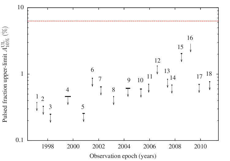
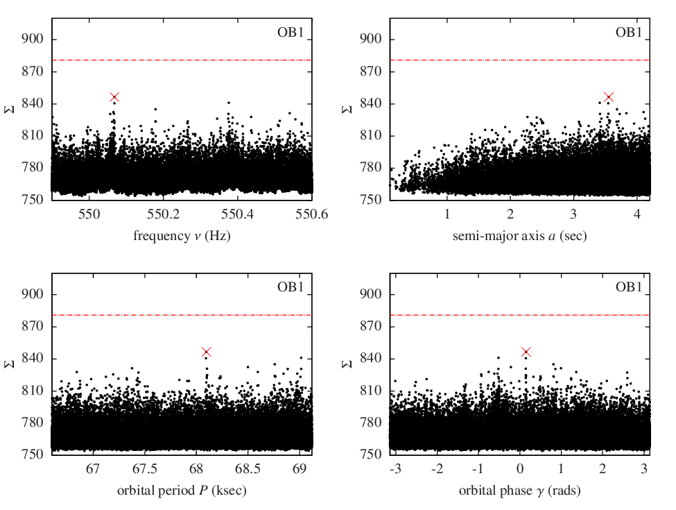
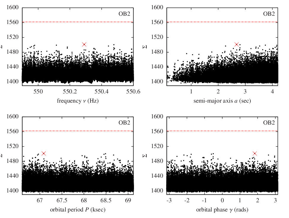
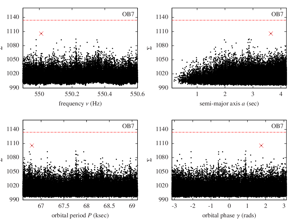
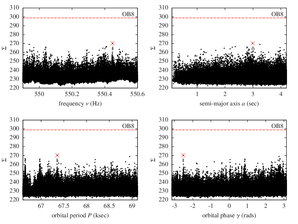
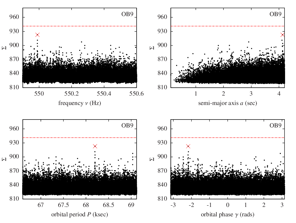
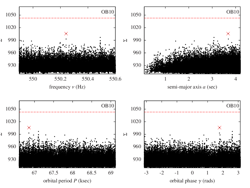
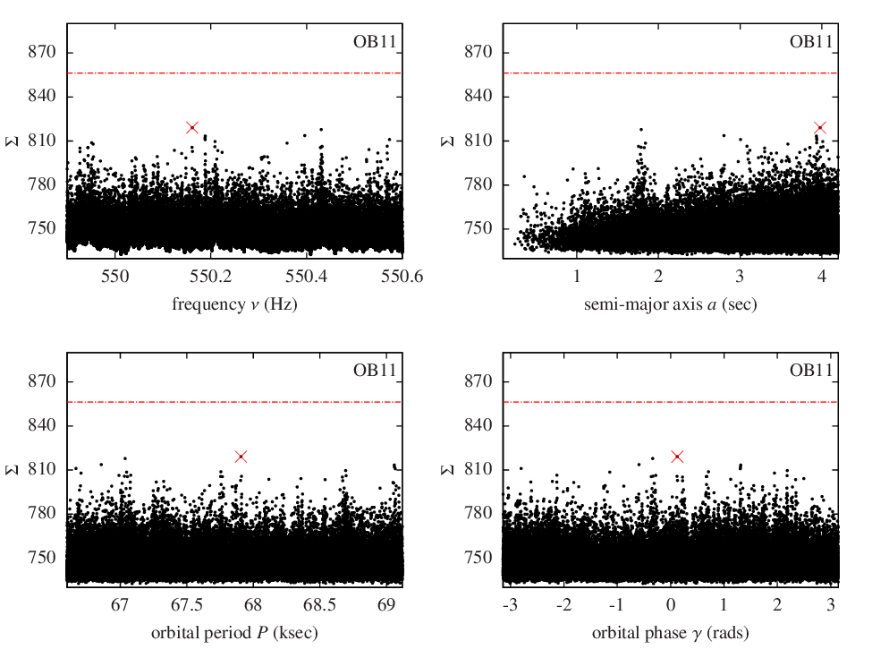
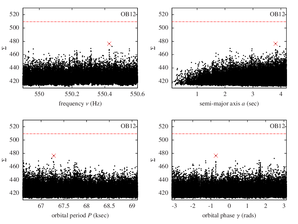
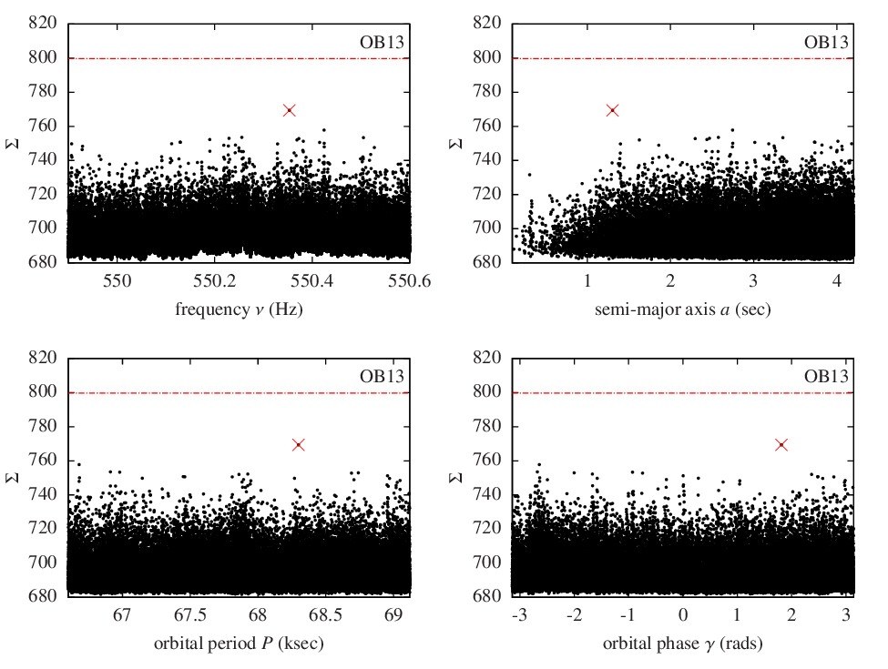
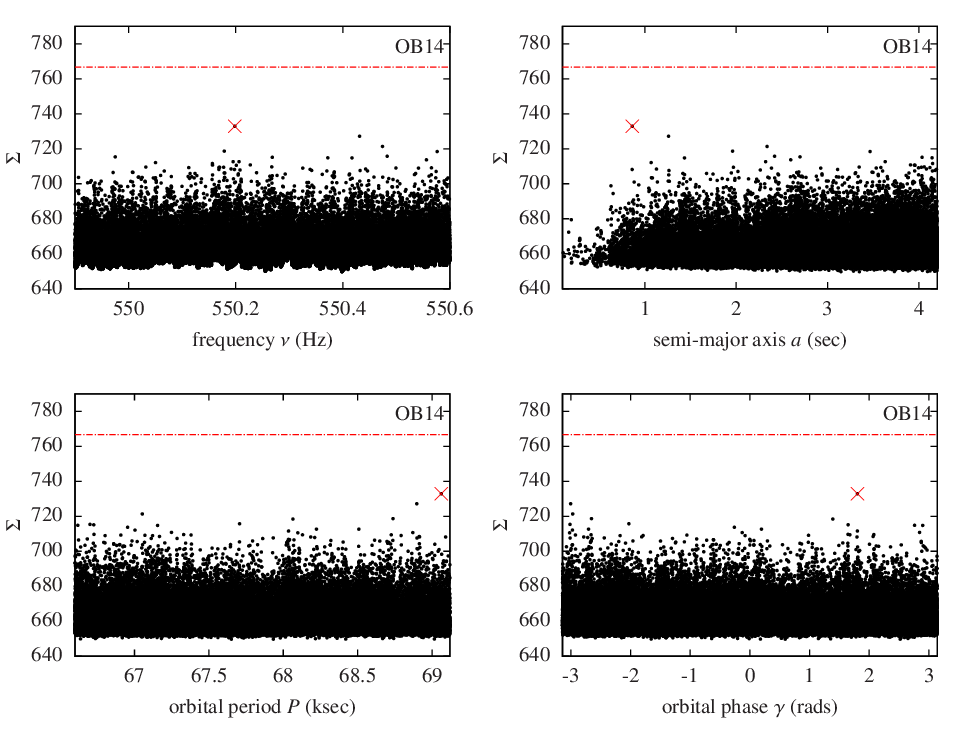
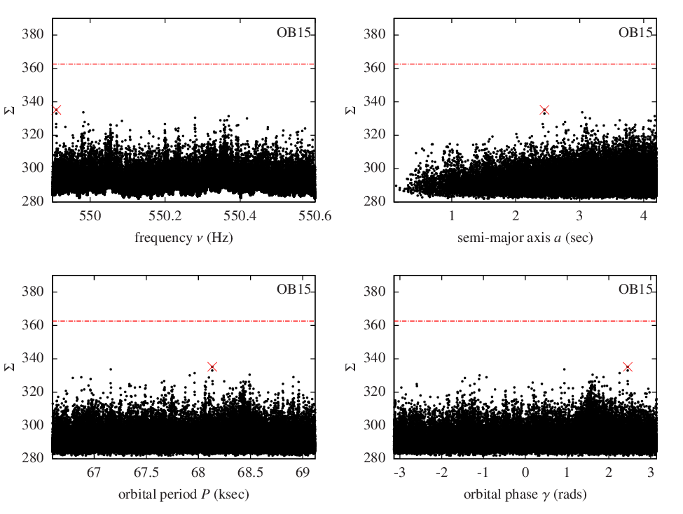
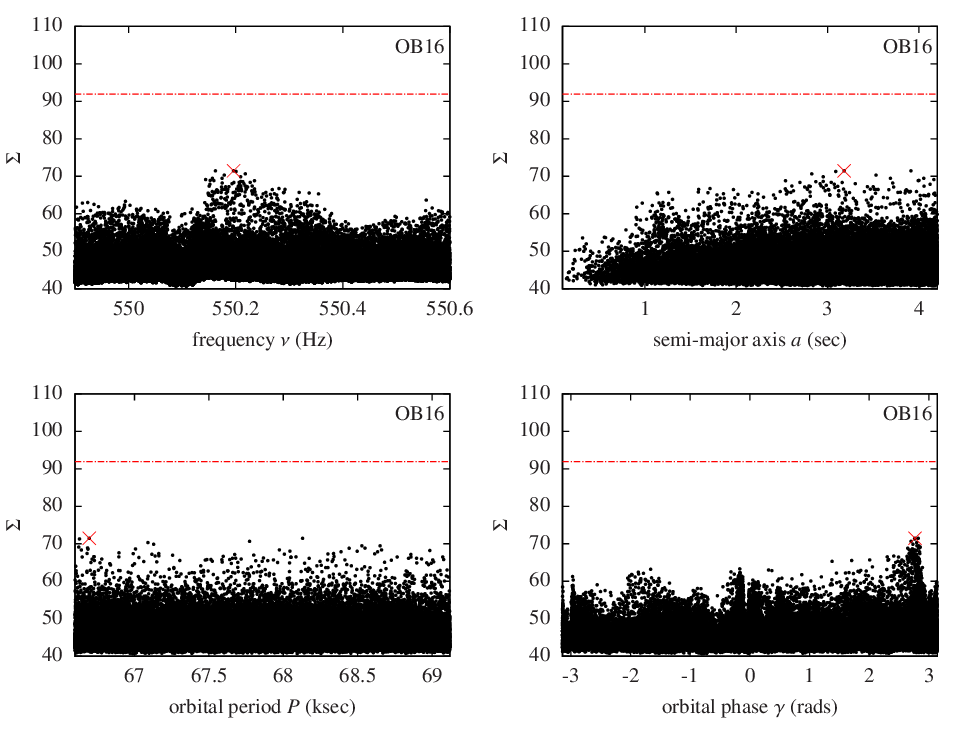
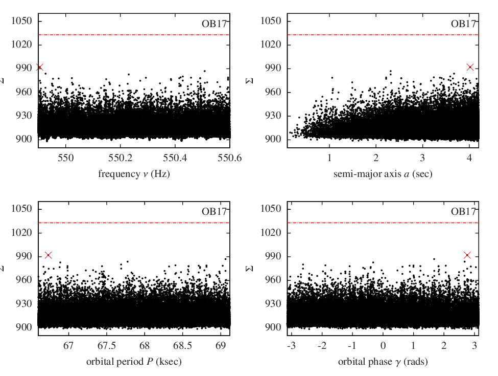
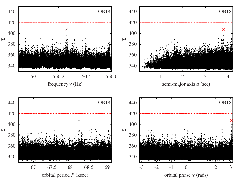
The application of our semi-coherent search to RXTE observations of Aql X–1 returned no evidence for the detection of pulsations in any of the 18 outbursts analysed. The corresponding search parameters, maximum detection statistics, and derived pulse fraction upper-limits are given in Table 7. The derived upper-limits form the main result of the analysis and in our most sensitive outburst we are able to limit the pulse fraction to ${<}0.249\%$ with $90\%$ confidence with the majority of outbursts return upper-limits ${<}1\%$. Results of the search in the most sensitive dataset (outburst 3) are shown in Fig. 2. In the following sections we describe the Aql X–1 search setup, the statistical analysis of the search results and the derivation of upper-limits, and finally we present a validation of the search using simulated signals.

Table 3The AQL X-1 outburst data parameters, estimated sensitivities and upper limits.

Outburst	GPS start	$\tau$ Ms	$\mathcal{N}\times 10^{6}$	$T$ ks	$M_{256}$	$n\times 10^{9}$	$\Sigma^{1\%}$	$A^{1\%}_{10\%}\,(\%)$	$\Sigma^{*}$	$P_{n}(\Sigma^{*})$	$A^{\mathrm{UL90\%}}\,(\%)$
1	540168821	1.478	46.8	77.06	301	13.04	880.9	0.396	846.6	0.8748	0.374
2	555367363	2.675	79.36	151	590	23.61	1562	0.352	1501	1.0	0.328
3	572925014	3.366	97.51	66.05	258	29.71	781.6	0.266	741.2	0.9996	0.249
4	610577860	14.47	78.44	371.2	1450	127.7	3498	0.441	3456	0.295	0.428
5	653812203	5.785	174.7	254.2	993	51.05	2478	0.269	2424	0.854	0.256
6	677384433	2.258	7.657	51.46	201	19.93	638.5	0.902	617.3	0.3949	0.867
7	697855525	3.46	18.75	103.7	405	30.53	1134	0.669	1106	0.4183	0.643
8	730230099	1.678	16.64	18.43	72	14.81	298.9	0.501	270.4	1.0	0.459
9	761167047	10.78	19.65	82.18	321	95.13	941.3	0.630	922.8	0.1728	0.611
10	796608483	4.422	20.41	93.7	366	39.02	1043	0.631	1006	0.9056	0.597
11	817073265	2.024	12.78	74.24	290	17.86	856.3	0.753	819.1	0.9703	0.705
12	838546705	1.389	2.698	38.66	151	12.26	509.4	1.426	476.5	0.999	1.328
13	863862099	1.756	8.983	68.35	267	15.5	799.7	0.881	769.4	0.7612	0.837
14	874369790	2.116	12.94	64.77	253	18.67	766.7	0.727	732.9	0.9374	0.685
15	897654239	3.321	0.9707	24.06	94	29.31	362.6	2.195	335.2	0.9986	2.038
16	921996024	0.007	0.186	2.816	11	0.0623	91.92	3.302	71.46	1.0	2.865
17	941531738	2.913	14.37	92.93	363	25.71	1033	0.746	992.1	0.9821	0.701
18	967988518	2.33	7.949	29.7	116	20.56	420.4	0.795	407.6	0.1649	0.770

• The column headings indicate the outburst index, the GPS start time of the outburst, the time span of the outburst observations, the total number of photons within the outburst, the total on-source data used, the number of 256s segments, the number of semi-coherent templates, the $1\%$ multi-trial false alarm threshold on $\Sigma$, the pulse fraction corresponding to a $1\%$ multi-trial false alarm and a $10\%$ false dismissal probability, the loudest measured detection statistic $\Sigma^{*}$, the multi-trial statistical significance of $\Sigma^{*}$, and the $90\%$ confidence pulse fraction upper-limit.

Figure 2.— The semi-coherent detection statistic $\Sigma$ plotted as a function of the 4-dimensional physical search space for the 3rd Aql X–1 outburst. The red cross indicates the location and value of the loudest detection statistic and the dashed horizontal line indicates the $1\%$ false alarm threshold.The results plotted here are the 100 loudest statistics in each $1$mHz sub-band.

Figure 3.— The $90\%$ confidence upper-limit on the pulse fraction for all outbursts as a function of observation. For each outburst the span of the solid horizontal bar represents the span of the observation. The dashed horizontal line indicates the pulse fraction observed by (Casella et al., 2008) and we have also indexed each outburst.

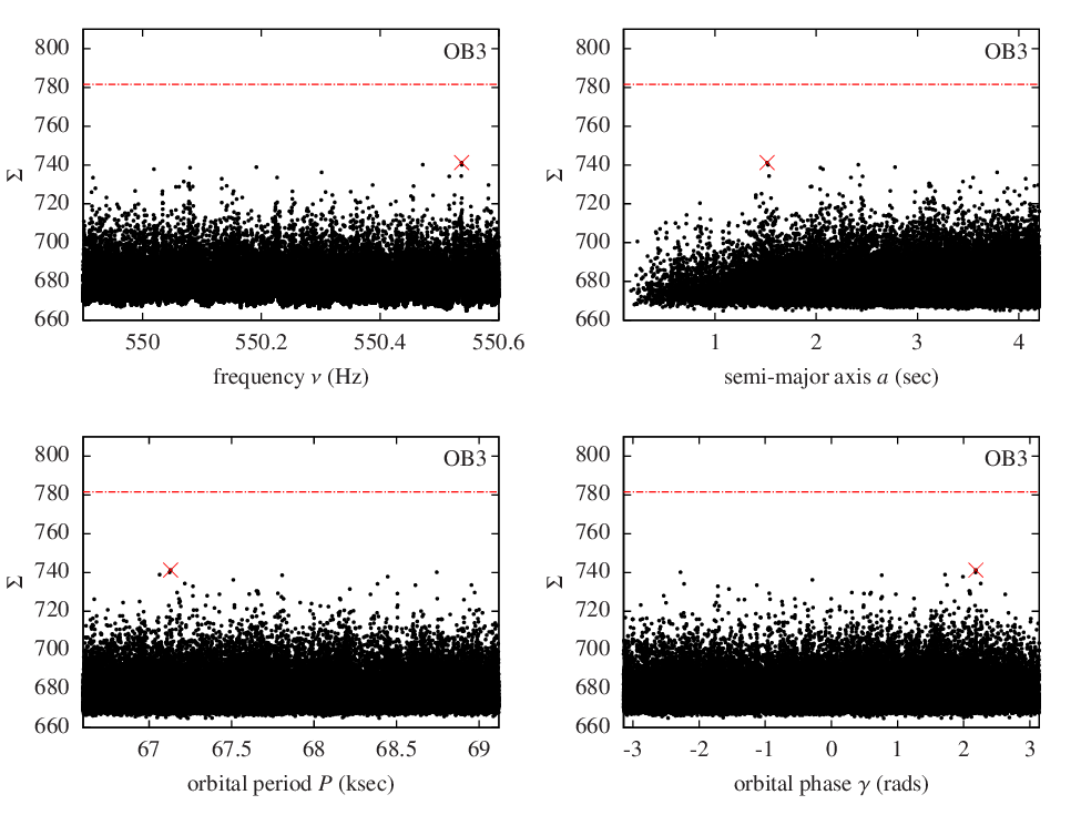
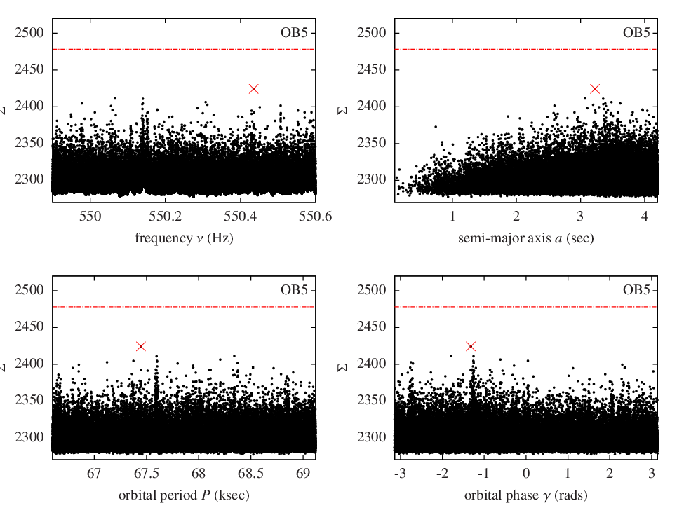
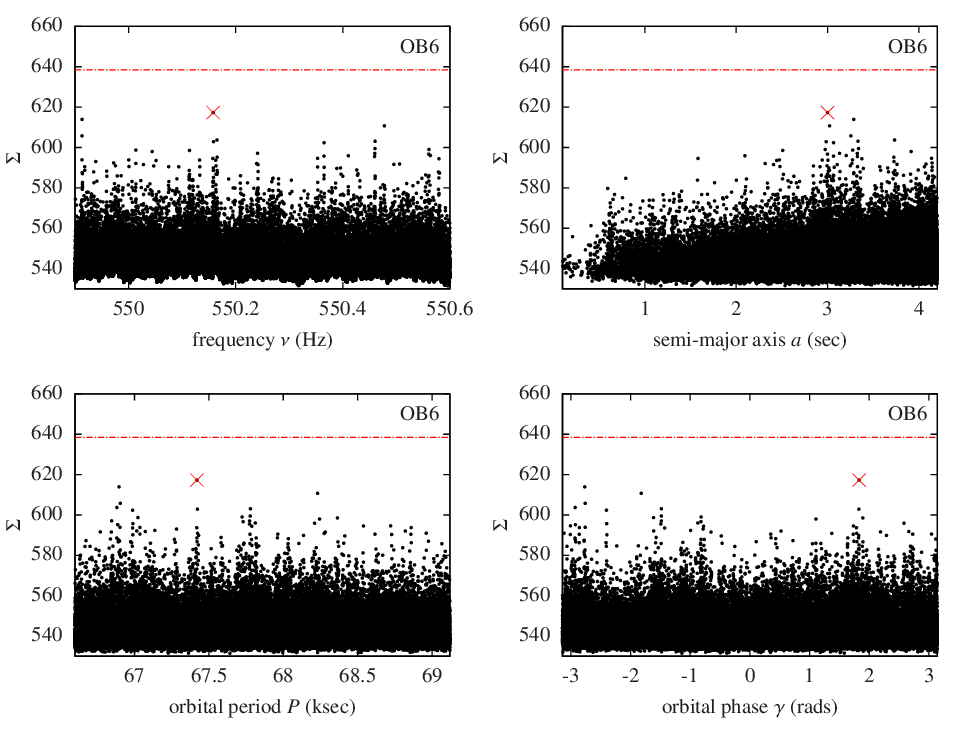
As can be seen from Fig. 2 and in the results from the other outbursts, there is a general trend for the detection statistic to be uniformly distributed with respect to the frequency, orbital period and orbital phase parameters. There is an clear increase in the occurrence of larger values of the statistic at higher values of the semi-major axis. This is to be expected since the density of templates also increases with semi-major axis. Hence, per unit semi-major axis there is a higher trials factor and correspondingly higher expectation in the loudest statistics recorded. We also note that only a subset of the $29.71\times 10^{9}$ results are plotted for outburst 3. The analysis is split into 700 separate $1$mHz sub-bands for processing in parallel using the ATLAS computer cluster (Aulbert, 2009) and in Fig. 2 we plot only the loudest 100 statistics per sub-band. Finally, we note that the reference time $t_{0}$ used to define the orbital phase $\gamma$ (see Sec. 6.1) is equal to the mid point of the observation span for each outburst.

For all outbursts a threshold value on the semi-coherent statistic is determined corresponding to a conservative approximation to a $1\%$ false alarm rate. In all cases no statistic exceeded this threshold and hence all results, even those exhibiting peak-like structures, were consistent with the null hypothesis. Peak-like structures are a natural feature of the noise (as verified in our simulations) and since our templates are, by design, highly correlated, any loud statistic values will be locally surrounded by similarly loud values. As an additional check we have performed a search on our most sensitive outburst (OB3) with a greatly extended orbital period parameter space ranging from 5 to 20 hours. Such short orbital periods increase the computational cost of the search by large factors (see Eq. 27) and to counteract this effect the coherent observation length was reduced to 32s. In this case, via Eq. 12 this corresponds to a reduction in the search sensitivity by $\sim\sqrt{2}$ . No statistically significant detection statistic values were recorded.

7.1. Aql X–1 search setup

Our choice of coherent observation time $T=256$ s was motivated by computational limitations specifically in the number of semi-coherent templates. From Eq. 6.4 we see that the number of templates is proportional to $T^{4}$ however, as we will show, the sensitivity of semi-coherent searches to the pulse fraction $A$ is proportional to $T^{1/4}$ (for a fixed total observation length). Hence, our value of $T$ has been chosen so as to achieve near optimal sensitivity while also keeping analysis times at manageable levels. Other freely chosen parameters of the analysis were the coherent and semi-coherent template bank mismatches which were both set to $\mu=0.1$. For the coherent template bank this represents the worst case mismatch and has a corresponding average value of $0.03$. For the semi-coherent case $\mu=0.1$ represents the mismatch achieved with a coverage probability $\eta=0.9$. The resulting average mismatch at any given parameter space location is $0.06$. Finally, for $s^{*}$, the maximum number of search dimensions on the approximate phase model, Eq. 23 was used to determine the required template spacing and then compared to the maximal parameter space width in the corresponding dimension. If the spacing was greater than the width then the dimension was not considered as part of the phase model. For our choice of mismatch and coherent observation time together with the Aql X–1 parameter space this resulted in a maximum value of $s^{*}=2$.

The RXTE observations of Aql X–1 span ${\sim}13$ years and are divided into 18 outbursts which we have chosen to analyse separately. The typical time span of an outburst is $\mathcal{O}(\text{few})$ Ms and together with our additional search parameter choices makes each analysis computationally tractable over a the timescale of ${\sim}$days using ${\sim}10^{3}$ nodes of a the ATLAS computer cluster. A single analysis of the entire dataset is made computationally very difficult by the linear relationship between the number of semi-coherent templates and the total observation span $\tau$. Such an analysis using the same coherent observation length would therefore be ${\sim}100$ times more intensive with a gain of only ${\approx}2$ in sensitivity to pulse fraction. Since our search is sensitive to signals of duration equal to or greater than our total observation, our choice of subdivision of analyses increases our sensitivity to signals of duration ${\geq}1$ Msec.

7.2. Statistical significance

A common problem in a templated wide parameter space search is the difficulty in estimating the number of templates that constitute statistically independent trials. By design we aim to have highly correlated templates, placed closely enough so as to not miss potential signals. By taking the actual number of templates as an upper-limit on the number of trials we can compute correspondingly conservative lower-limits on detection significance. Let the probability of obtaining a value of our statistic greater than or equal to $\Sigma$ be $P(\Sigma)$ in the case of noise alone and a single trial. The distribution of $\Sigma$ for noise only is known to be the central $\chi^{2}$ distribution with $2M$ degrees of freedom and hence

$$P(\Sigma)=1-\frac{\gamma\left(M,\frac{\Sigma}{2}\right)}{\Gamma(M)}$$ (30)

where $\gamma$ and $\Gamma$ represent incomplete and complete gamma functions respectively. With an upper-limit on the number of independent trials equal to $n$ we can state that

$$P_{n}(\Sigma)\leq 1-\left(1-P(\Sigma)\right)^{n}$$ (31)

is the probability of getting 1 or more events greater than $\Sigma$ after $n$ trials. We can now equate this to a multi-trial false alarm probability $P_{\text{fa}}$ and solve for $\Sigma$ giving

$$\Sigma^{*}\leq P^{-1}\left((1-P_{\text{fa}})^{1/n}-1\right)$$ (32)

where $P^{-1}$ is the inverse function of the single trial probability. We show in Table 7 the outburst parameters and the expected sensitivities to pulse fraction amplitude for a multi-trial false alarm of $1\%$ and a false dismissal probability of $10\%$. We also give upper-limits on the statistical significance of the loudest events in each outburst.

7.3. Upper-limits on pulse fraction

Given the results of our analyses are consistent with the null hypothesis we proceed to set upper-limits on the pulse fraction in each outburst. We base this on our loudest statistic and ask the question “what is the value of $A$ such that with probability $C$ we would have achieved a detection statistic greater than, or equal to, the maximum value observed $\Sigma^{*}$”. Using the expected distribution of the detection statistic in the presence of a signal (the properties of which are given in Eq. 10a) we solve the following for $A$:

$$C(\Sigma^{*},\mu^{*})= \int\limits_{\Sigma^{*}}^{\infty}d\Sigma\int\limits_{0}^{1}d\mu_{\Sigma}\int\limits_{0}^{\mu^{*}}d\mu^{(1)}_{\Lambda},\ldots\int\limits_{0}^{\mu^{*}}d\mu^{(M)}_{\Lambda}$$

$$\chi^{2}_{2M}\left[\Sigma,\lambda(A,\mu_{\Sigma},\left\{\mu_{\Lambda}\right\})\right]p(\mu_{\Sigma})\prod_{m=1}^{M}p(\mu_{\Lambda}^{(m)}).$$ (33)

where $\mu^{*}$ is the maximal coherent template mismatch and $p(\mu_{\Sigma})$ and $p(\mu_{\Lambda}^{(m)})$ are the prior mismatch distributions for the semi-coherent and coherent template banks respectively. The non-centrality parameter $\lambda$ of the non-central $\chi^{2}$ likelihood function is simply the sum of squared SNRs from each segment after accounting for mismatches such that

$$\lambda(A,\mu_{\Lambda},\mu_{\Sigma})=\frac{NA^{2}}{2}(1-\mu_{\Sigma})\sum_{m=1}^{M}\langle R\rangle_{m}(1-\mu^{(m)}_{\Lambda}).$$ (34)

We marginalize the likelihood over the possible mismatches expected from both the coherent and semi-coherent template banks. This expression is an accurate approximation despite the fact that we have assumed the same average background rate for each segment. For the hypercubic grid of coherent templates we know that the probability distribution on mismatch for a single random location in 2-dimensions is given by

$$p(\mu_{\Lambda})=\begin{dcases*}\pi/2&if $\mu\leq 1/2$\\ \frac{\pi}{2}-2\cos^{-1}\left(\frac{1}{\sqrt{2\mu_{\Lambda}}}\right)&if $1/2<\mu<1$.\end{dcases*}$$ (35)

For the semi-coherent bank a single statistic is affected by only one realization of mismatch and in 4-dimensions is governed by the distribution

$$p(\mu_{\Sigma},\eta)=-2\log\left(1-\eta\right)\frac{\mu_{\Sigma}}{\mu^{*}}(1-\eta)e^{-(\mu_{\Sigma}/\mu^{*})^{2}}.$$ (36)

Using Eq. 7.3 we are then able to answer our upper-limit question and claim an amplitude on pulse fraction above which we confidently rule out the true signal value. The corresponding values for each Aql X–1 outburst are given in Table 7 in the final column. We can also use Eq. 7.3 to compute an expected search sensitivity based on a predefined false alarm and false dismissal probability. In this case we simply replace the input measured semi-coherent statistic with the value of $\Sigma^{P_{\text{fa}}}$ computed via Eq. 32 and equate our upper-limit confidence $C$ to the complement of the false dismissal probability. The corresponding values of $A$ for a false alarm probability of $1\%$ and a false dismissal of $10\%$ ($C=90\%$) are also given Table 7.

7.4. Pulse Search Validation

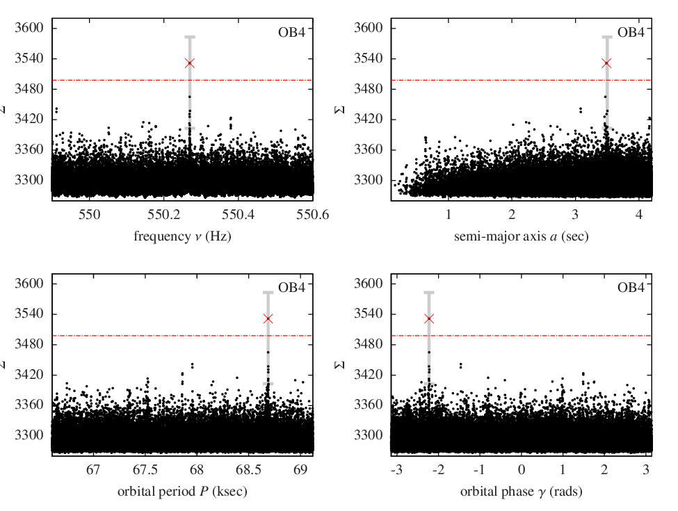
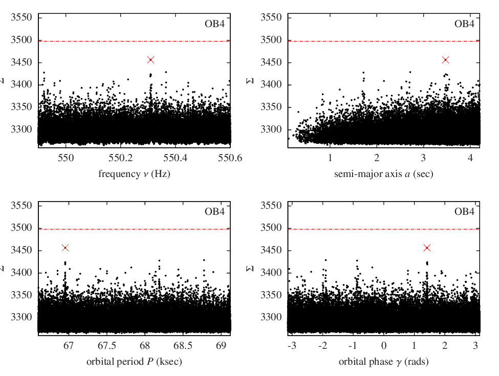
To verify our claimed sensitivity (pulse fraction semi-amplitude of $0.3\%$) and to validate our search algorithm, we performed a blind test in which an artificial signal of amplitude close to the claimed sensitivity was injected into a random outburst. The binary and spin parameters of the signal were randomly chosen by one author from within the range reported in Table 2 and with a semi-amplitude of $0.4\%$. The same author then replaced one of the first six outbursts with an artificial outburst containing the signal while maintaining the statistical properties of the original outburst. Then the first six outbursts (including the artificial one) were submitted to the other author who, without knowing which outburst and which binary/spin parameters were selected, proceeded to apply the search algorithm to the datasets. The results show that the outburst containing the fake signal (outburst 4) was detected with a false alarm probability of $\leq 3.6\times 10^{-5}$ and would have therefore been claimed as a detection.

We are able to make relatively accurate estimates of the parameter uncertainties using Bayes theorem together with some simplifying assumptions. In the specific case where the prior probability distributions on the search parameters are uniform we find that the posterior distribution on the search parameters is proportional to the likelihood function.

The first of our simplifications is to use only the loudest template to perform any inference and to treat the pulse fraction separately from the phase parameters. Our estimate of the true pulse fraction value is therefore obtained according to

$$p(A|\Sigma^{*})\propto\int\limits_{0}^{\infty}d\mu_{\Sigma}\chi^{2}_{2M}\left(\Sigma^{*},\lambda\left(A,\{\mu_{\Lambda}\},\mu_{\Sigma}\right)\right)p(\mu_{\Sigma})$$ (37)

where we include a marginalization over the unknown value of the true semi-coherent mismatch. From this posterior we then take the median as our pulse fraction estimate $A^{*}$ and compute the minimal $68\%$ confidence range as our uncertainty (see Table 4).

For the phase parameters we adopt the same approach but keep the amplitude parameter assumed known with value $A^{*}$. The uncertainties quoted in Table 4 are therefore obtained from marginalizing the posterior distribution which in our specific case is

$$p(\bm{\theta}|\Sigma^{*},\bm{\theta}^{*})\propto\chi^{2}_{2M}\left(\Sigma^{*}|,\lambda\left(A^{*},\{\mu_{\Lambda}\},\mu_{\Sigma}\left(\Delta\phi\left(\bm{\theta},\bm{\theta}^{*}\right)\right)\right)\right)$$ (38)

where the semi-coherent mismatch $\mu_{\Sigma}$ is now expressed as a function of the phase offsets $\Delta\phi(\bm{\theta},\bm{\theta}^{*})$ caused by the mismatch between the phase model of the loudest event $\bm{\theta}^{*}$ and that of the unknown true value $\bm{\theta}$. In Fig. 4 we show that in addition to detection, all the binary and spin parameters were correctly recovered.

Figure 4.— The semi-coherent detection statistic $\Sigma$ plotted as a function of the 4-dimensional physical search space for an artificially generated outburst based on the 4th Aql X–1 outburst and containing an artificial signal. The red cross indicates the location and value of the loudest detection statistic and the dashed horizontal line indicates the $1\%$ false alarm threshold. The y-axis span bounded by the grey lines indicate the 1-$\sigma$ confidence region within which we expect the $\Sigma$ value of the simulated signal’s loudest template to lie. The x-axis location of the grey lines indicate the parameters of the artificial signal.

Table 4The artificial signal parameters and their estimates.

Parameter	Units	Value	Estimate	Uncertainty
$A$	$\%$	0.40	0.43	(0.39,0.46)
$f$	Hz	550.27	550.26929	0.0013
$a$	s	3.5	3.487	0.035
$P$	hr	19.08	19.08005	0.00063
$\gamma$	rads	4.058352257914	4.0579	0.0144
Max detection statistic $\Sigma^{*}$			3562.8
Expected $68\%$ $\Sigma^{*}$ range			$(3403,3583)$
Statistical significance $P_{\Sigma^{*}}$			$\leq 5.25\times 10^{-4}$

8. Discussion

The semi-coherent search presented in this paper represents the first complete search of pulsations in Aql X–1, carried for all 18 outbursts recorded with high time resolution data. This search places strong constrains on the presence of pulsations for 15 out of 18 outbursts, with upper limits of ${\sim}0.3-0.9\%$. In the remaining three outbursts the upper limits are of the order of 1–3% (due to the short duration of the observations).

The non-detection of pulsations in Aql X–1 adds to previous deep pulse searches carried on 15 low mass X-ray binaries (Vaughan et al., 1994; Dib et al., 2005). Vaughan et al. (1994) analysed Ginga data of 15 bright Z and atoll sources with the quadratic coherence recovery technique and placed upper limits between 0.3% (in Sco X-1) and 8% (4U 1608-52). Dib et al. (2005) used acceleration searches on the ultra-compact source 4U 1820-30 (which was also among the 15 sources analysed by Vaughan et al. 1994) and placed upper limits of the order of 0.8% on the pulse amplitude.

Even if many other LMXBs have never shown pulsations, the non-detections in Aql X–1 are somehow surprising. Indeed this source has shown pulsations for ${\sim}150$ seconds during its 1998 outburst (outburst 3 in table 7) out of a total observing time of 1.7 Msec, so that pulsations are present in just 0.009% of the observed time). Casella et al. (2008) reported a fractional semi-amplitude of ($1.9\pm 0.2)\%$ for the single pulse episode in the full RXTE energy band (2–60 keV). The pulse semi-amplitude in the energy band considered here (7–25 keV) reaches a value of ${\sim}6.5\%$ whereas our upper limits on the pulsed amplitude in the same outburst reach a value of 0.26%. The high pulsed amplitude of the signal makes it difficult to believe that very weak pulses still exist and remain undetected below our detection threshold, since this would require a sudden jump by more than a factor of 25 in pulsed amplitude without other pulse episodes with intermediate values being present (which we would have detected). Our results support therefore the idea that Aql X–1 has shown a single pulse episode.

Casella et al. (2008) discussed several possible scenarios to explain the single pulse episode. In the following we review those mechanisms and we explore new possibilities emerged in the last few years.

The presence of a dipolar magnetosphere with a field of $10^{7}$–$10^{9}$ G, comparable to that seen in radio and other AMXPs seems hard to justify since the interaction between the field lines and the plasma would very likely break the high degree of symmetry required to avoid the production of pulsations. On the other hand weak pulsations are seen in some AMXPs, most remarkably pulsations at the 0.4% level (0.3% rms) where detected in the intermittent pulsar HETE J1900.1–2455 (Galloway et al., 2008; Patruno, 2012). Patruno (2012) reported that in that particular source the pulsations are seen at the 0.4% level only very intermittently and suggested that this behaviour is related to the screening of the magnetic field. In Aql X–1 such gradual screening cannot be the explanation for the lack of pulsations because the single 150 s is preceded and followed by the absence of pulsations. Furthermore the magnetic field cannot re-emerge and be screened on such short timescales, which are thought to be on the order of the Ohmic diffusion timescale (typically 1-10 years (Cumming et al., 2001)).

An alternative model suggests that the lack of pulsations is due to the nearly perfect alignment of magnetic and spin axis. Lamb et al. (2009a, b) modeled the emission of a 400 Hz AMXP, with an hot spot with an angular size of $25^{\circ}$ and a neutron star of 1.4$\,M_{\odot}$ and $10$ km in radius. According to this model, the pulse amplitude is smaller than our most stringent upper limits only if the observer inclination is smaller than about 10 degrees and the hot spot misalignment angle is less than 2 degrees (see Figure 1 in both Lamb et al. 2009a and Lamb et al. 2009b, with the caveat that Aql X–1 is spinning at 550 Hz). Although initially believed to be a low inclination binary (Garcia et al., 1999; Shahbaz et al., 1998), Aql X–1 is now thought to have an inclination with $36^{\circ}<i<70^{\circ}$ (Welsh et al., 2000). In this case the hot spot misalignment needs to be substantially less than 2 degrees. Since the 150 s pulse episode had a fractional amplitude of ${\sim}6\%$ (7–25 keV), which requires a misalignment of about $15^{\circ}$, it seems difficult to conceive a mechanism to keep the hot spot almost completely locked to the rotational axis for the greatest majority of its lifetime and then justify a sudden large drift of $15^{\circ}$ or more for just 150 seconds. Also, numerical MHD simulations of hot spots on accreting neutron stars (Kulkarni & Romanova, 2013) show that such rigid locking is nearly impossible to achieve as hot spots move and change shape substantially during the accretion process.

Another possibility is that Aql X–1 spends most of its time accreting via a Rayleigh-Taylor instability. Such interchange instability has been observed to emerge in numerical MHD simulations of AMXPs (Kulkarni & Romanova, 2008) when the mass accretion rate overcomes a certain threshold. Aql X–1 is the most luminous AMXP known, reaching peak luminosities $>10^{37}\rm\,erg\,s^{-1}$ thus indicating a high mass accretion rate. However, it is not clear why the pulsations are not seen during the outbursts rises, or why the single pulse episode is observed when the luminosity has almost reached its maximum (when the mass accretion rate is higher and thus pulsations should not be expected).

The smearing of the pulsation due to gravitational lensing is also a possibility considered in the literature (Wood et al., 1988; Özel, 2009). However, also in this case the presence of one single moderately high amplitude pulsation seems to require a strong fine tuning of the geometric configuration of the hot spot and neutron star parameters and can almost certainly be ruled out. Finally, smearing of pulsations via electron scattering (Brainerd & Lamb, 1987; Titarchuk et al., 2002) seems also difficult to justify because no spectral variation are observed between the pulse and non-pulsating phases (see  Casella et al. 2008; Altamirano & Casella 2008 for a discussion).

None of the mechanisms above, which do require a dipolar magnetosphere (a multipolar magnetosphere would run into similar problems), seem to explain the sharp contrast between the pulsating and non-pulsating phases of Aql X–1. Although the pulse non-detections make any scenario highly speculative, we suggest that the lack of pulsations is related to the lack of a strong magnetosphere. We can speculate that Aql X–1 has either no magnetosphere or a very weak one which is unable to influence the accretion flow in any significant way. The single pulse episode must therefore be ascribed to some other phenomenon, unrelated to channeled accretion.

Modes of oscillations have been suggested as a possible mechanism for the pulse episode of Aql X–1 (Casella et al., 2008). An oscillation mode with azimuthal number $m$ and frequency $\nu_{\text{mod}}$ would give an observed frequency $\nu_{\text{obs}}$ given a spin frequency $\nu$:

$$\nu_{\text{obs}}=m\,\nu\,+\,\nu_{\text{mod}}$$ (39)

Since $\nu_{\text{obs}}=550.273$ Hz and since we know the approximate spin frequency within ${\sim}1\,$Hz from burst oscillations (Zhang et al., 1998), then an $m=1$ mode with $\nu_{\text{mod}}{\sim}1$ Hz can explain the observations. Any shorter mode frequency would still be a valid possibility down to a frequency of $\nu_{\text{mod}}=1/\Delta\,T={\sim}7\times 10^{-3}$ Hz, where $\Delta\,T{\sim}150$ s is the duration of the single pulse episode. However, even if the frequencies have plausible values, this mechanism remains difficult to justify. Indeed is not clear what might have excited the mode since no burst or any other relevant event has been recorded close or during the pulse episode.

9. Conclusions

We have analyzed the entire RXTE/PCA datasets available for the LMXB Aql X–1 to search for pulsations with a new technique known as semi-coherent search. We have reached an unprecedented sensitivity that reaches a fractional amplitude of 0.3%. We detect no pulsations beside the already known 150-s long episode detected in 1998. Out typical upper limits on the fractional amplitude span a range of 0.3-0.9% (semi-amplitude) in the 7–25 keV energy range. By considering all possible known pulse formation mechanisms we conclude that Aql X–1 is unlikely to be accreting from an extended magnetosphere and some other exotic explanation, yet to be identified, is required to justify the observed behaviour.

Appendix A Additional results

Figure 5.— The semi-coherent detection statistic $\Sigma$ plotted as a function of the 4-dimensional physical search space for the 1st, 2nd, 4th, 5th, 6th and 7th Aql X–1 outbursts. The red crosses indicates the location and value of the loudest detection statistic and the dashed horizontal lines indicates the $1\%$ false alarm thresholds.

Figure 6.— The semi-coherent detection statistic $\Sigma$ plotted as a function of the 4-dimensional physical search space for the 8th–13th Aql X–1 outbursts. The red crosses indicates the location and value of the loudest detection statistic and the dashed horizontal lines indicates the $1\%$ false alarm thresholds.

Figure 7.— The semi-coherent detection statistic $\Sigma$ plotted as a function of the 4-dimensional physical search space for the 14th–18th Aql X–1 outbursts. The red crosses indicates the location and value of the loudest detection statistic and the dashed horizontal lines indicates the $1\%$ false alarm thresholds.

References

- Altamirano & Casella (2008) Altamirano, D., & Casella, P. 2008, in American Institute of Physics Conference Series, Vol. 1068, American Institute of Physics Conference Series, ed. R. Wijnands, D. Altamirano, P. Soleri, N. Degenaar, N. Rea, P. Casella, A. Patruno, & M. Linares, 63–66
- Altamirano et al. (2008) Altamirano, D., Casella, P., Patruno, A., Wijnands, R., & van der Klis, M. 2008, ApJ, 674, L45
- Aulbert (2009) Aulbert, C. & Fehrmann, H. 2009, Max-Planck-Gesellschaft Jahrbuch
- Balasubramanian et al. (1996) Balasubramanian, R., Sathyaprakash, B. S., & Dhurandhar, S. V. 1996, Phys. Rev. D, 53, 3033
- Basko & Sunyaev (1976) Basko, M. M., & Sunyaev, R. A. 1976, MNRAS, 175, 395
- Bildsten & Brown (1997) Bildsten, L., & Brown, E. F. 1997, ApJ, 477, 897
- Bisnovatyi-Kogan & Komberg (1974) Bisnovatyi-Kogan, G. S., & Komberg, B. V. 1974, Soviet Ast., 18, 217
- Brady & Creighton (2000) Brady, P. R., & Creighton, T. 2000, Phys. Rev. D, 61, 082001
- Brainerd & Lamb (1987) Brainerd, J., & Lamb, F. K. 1987, ApJ, 317, L33
- Campana et al. (2013) Campana, S., Coti Zelati, F., & D’Avanzo, P. 2013, MNRAS, 432, 1695
- Casella et al. (2008) Casella, P., Altamirano, D., Patruno, A., Wijnands, R., & van der Klis, M. 2008, ApJ, 674, L41
- Chevalier & Ilovaisky (1991) Chevalier, C., & Ilovaisky, S. A. 1991, A&A, 251, L11
- Chevalier & Ilovaisky (1998) —. 1998, IAU Circ., 6806, 2
- Cumming et al. (2001) Cumming, A., Zweibel, E., & Bildsten, L. 2001, ApJ, 557, 958
- Dib et al. (2005) Dib, R., Ransom, S. M., Ray, P. S., Kaspi, V. M., & Archibald, A. M. 2005, ApJ, 626, 333
- Galloway et al. (2008) Galloway, D. K., Morgan, E. H., & Chakrabarty, D. 2008, in AIPC Series, Vol. 1068, A Decade of Accreting Millisecond X-Ray Pulsars, ed. R. Wijnands, D. Altamirano, P. Soleri, N. Degenaar, N. Rea, P. Casella, A. Patruno, & M. Linares, 55–62
- Galloway et al. (2007) Galloway, D. K., Morgan, E. H., Krauss, M. I., Kaaret, P., & Chakrabarty, D. 2007, ApJ, 654, L73
- Garcia et al. (1999) Garcia, M. R., Callanan, P. J., McCarthy, J., Eriksen, K., & Hjellming, R. M. 1999, ApJ, 518, 422
- Gavriil et al. (2007) Gavriil, F. P., Strohmayer, T. E., Swank, J. H., & Markwardt, C. B. 2007, ApJ, 669, L29
- Ghosh & Lamb (1978) Ghosh, P., & Lamb, F. K. 1978, ApJ, 223, L83
- Ghosh & Lamb (1979) —. 1979, ApJ, 234, 296
- Ghosh et al. (1977) Ghosh, P., Pethick, C. J., & Lamb, F. K. 1977, ApJ, 217, 578
- Jahoda et al. (2006) Jahoda, K., Markwardt, C. B., Radeva, Y., et al. 2006, ApJS, 163, 401
- Kaaret et al. (2006) Kaaret, P., Morgan, E. H., Vanderspek, R., & Tomsick, J. A. 2006, ApJ, 638, 963
- Kulkarni & Romanova (2008) Kulkarni, A. K., & Romanova, M. M. 2008, MNRAS, 386, 673
- Kulkarni & Romanova (2013) —. 2013, MNRAS, 433, 3048
- Lamb et al. (2009a) Lamb, F. K., Boutloukos, S., Van Wassenhove, S., et al. 2009a, ApJ, 706, 417
- Lamb et al. (2009b) —. 2009b, ApJ, 705, L36
- Messenger (2011) Messenger, C. 2011, Phys. Rev. D, 84, 083003
- Owen (1996) Owen, B. J. 1996, Phys. Rev. D, 53, 6749
- Owen & Sathyaprakash (1999) Owen, B. J., & Sathyaprakash, B. S. 1999, Phys. Rev. D, 60, 022002
- Özel (2009) Özel, F. 2009, ApJ, 691, 1678
- Papitto et al. (2013) Papitto, A., D’Aì, A., Di Salvo, T., et al. 2013, MNRAS, 429, 3411
- Patruno (2012) Patruno, A. 2012, ApJ, 753, L12
- Patruno & Watts (2012) Patruno, A., & Watts, A. L. 2012, ArXiv e-prints
- Poutanen & Gierliński (2003) Poutanen, J., & Gierliński, M. 2003, MNRAS, 343, 1301
- Ransom et al. (2002) Ransom, S. M., Eikenberry, S. S., & Middleditch, J. 2002, AJ, 124, 1788
- Ruderman (1991) Ruderman, M. 1991, ApJ, 366, 261
- Shahbaz et al. (1998) Shahbaz, T., Thorstensen, J. R., Charles, P. A., & Sherman, N. D. 1998, MNRAS, 296, 1004
- Titarchuk et al. (2002) Titarchuk, L., Cui, W., & Wood, K. 2002, ApJ, 576, L49
- Tudose et al. (2013) Tudose, V., Paragi, Z., Yang, J., et al. 2013, The Astronomer’s Telegram, 5158, 1
- van Straaten et al. (2003) van Straaten, S., van der Klis, M., & Méndez, M. 2003, ApJ, 596, 1155
- Vaughan et al. (1994) Vaughan, B. A., van der Klis, M., Wood, K. S., et al. 1994, ApJ, 435, 362
- Welsh et al. (2000) Welsh, W. F., Robinson, E. L., & Young, P. 2000, AJ, 120, 943
- Wijnands & van der Klis (1998) Wijnands, R., & van der Klis, M. 1998, Nature, 394, 344
- Wood et al. (1988) Wood, K. S., Ftaclas, C., & Kearney, M. 1988, ApJ, 324, L63
- Zhang et al. (1998) Zhang, W., Jahoda, K., Kelley, R. L., et al. 1998, ApJ, 495, L9+