Nonparametric estimation of the division rate of an age dependent branching process

Abstract.

We study the nonparametric estimation of the branching rate $B(x)$ of a supercritical Bellman-Harris population: a particle with age $x$ has a random lifetime governed by $B(x)$; at its death time, it gives rise to $k\geq 2$ children with lifetimes governed by the same division rate and so on. We observe in continuous time the process over $[0,T]$. Asymptotics are taken as $T\rightarrow\infty$; the data are stochastically dependent and one has to face simultaneously censoring, bias selection and non-ancillarity of the number of observations. In this setting, under appropriate ergodicity properties, we construct a kernel-based estimator of $B(x)$ that achieves the rate of convergence $\exp(-\lambda_{B}\frac{\beta}{2\beta+1}T)$, where $\lambda_{B}$ is the Malthus parameter and $\beta>0$ is the smoothness of the function $B(x)$ in a vicinity of $x$. We prove that this rate is optimal in a minimax sense and we relate it explicitly to classical nonparametric models such as density estimation observed on an appropriate (parameter dependent) scale. We also shed some light on the fact that estimation with kernel estimators based on data alive at time $T$ only is not sufficient to obtain optimal rates of convergence, a phenomenon which is specific to nonparametric estimation and that has been observed in other related growth-fragmentation models.

Mathematics Subject Classification (2010): 35A05, 35B40, 45C05, 45K05, 82D60, 92D25, 62G05, 62G20.

Keywords: Growth-fragmentation, cell division, nonparametric estimation, bias selection, minimax rates of convergence, Bellman-Harris processes.

1. Introduction

1.1. Motivation

Structured models have been paid particular attention over the last few years, both from a probabilistic and an applied analysis angle, in particular with a view toward a better understanding of population evolution in mathematical biology (see for instance the textbook by Perthame [21] and the references therein). In this context, a more specific focus and need for statistical methods has emerged recently (e.g. Doumic et al. [9, 8, 7] and the references therein) and this is the topic of the present paper. If $x$ denotes a so-called structuring variable – for instance age, size, any measure of variability or DNA content of a cell or bacteria, and if $n(t,x)$ denotes the number or density of cells at time $t$ of a population starting from a single ancestor at time $t=0$, a sound mathematical model can be obtained by specifying an evolution equation for $n(t,x)$.

Consider for instance the paradigmatic problem of age-dependent cell division, where the evolution of $n(t,x)$ is given by the simplest transport-fragmentation equation

(1) $$\left\{\begin{array}[]{l}\displaystyle\frac{\partial}{\partial t}n(t,x)+\frac{\partial}{\partial x}n(t,x)+B(x)n(t,x)=0\\ \\ n(t,0)=m\int_{0}^{\infty}B(y)n(t,y)dy,\;\;t>0,\;\;n(0,x)=\delta_{0},\end{array}\right.$$

where $\delta_{0}$ denotes the Dirac mass at point $0$. In this model, each cell dies according to a division rate $x\leadsto B(x)$ that depends on its age $x$ only (a living cell of age $x$ has probability $B(x)dx$ of dying in the interval $[x,x+dx]$) and, at its time of death, it gives rise to $m\geq 2$ children at its time of death. The parameters $(m,B)$ specify the so-called age-dependent model.

In this seemingly simple context, we wish to draw statistical inference on the division rate function $x\leadsto B(x)$ and on $m$ in the most rigorous way, when we observe the evolution of the population through time and when the shape of the function $B$ can be arbitrary, to within a prescribed smoothness class, i.e. in a nonparametric setting. In order to do so, we transfer the deterministic description (1) into a probabilist model that consists of a system of (non-interacting) particles specified by a probability distribution $p$ on the integers (the offspring distribution) and a probability density $f$ on $[0,\infty)$. A particle has a random lifetime drawn according to $f(x)dx$; at the time of its death, it gives rise to $k$ children with probability $p_{k}$ (with $p_{0}=p_{1}=0$), each child having independent lifetimes distributed as $f(x)dx$, and so on. The resulting process is a classical supercritical Bellman-Harris, see for instance the textbooks of Harris [12] or Athreya and Ney [2]. It is described by a piecewise deterministic Markov process

(2) $$X(t)=\big{(}X_{1}(t),X_{2}(t),\ldots\big{)},\quad t\geq 0,$$

with values in $\bigcup_{k\geq 1}[0,\infty)^{k}$, where the $X_{i}(t)$’s denote the (ordered) ages of the living particles at time $t$. The formal link between $X(t)$ and $n(t,x)$ is obtained via $n(t,x)=\mathbb{E}\big{[}\sum_{i=1}^{\infty}\delta_{X_{i}(t)=x}\big{]}$ which has to be understood in a weak (measure) sense, i.e. the empirical measure (in expectation) of the particle system and solves Equation (1), we refer to [20].

The correspondence between $(m,B)$ and $(f,p)$ is given by

(3) $$B(x)=\frac{f(x)}{1-\int_{0}^{x}f(s)ds},\;x\in[0,\infty),\;\;\text{and}\;\;m=\sum_{k\geq 2}kp_{k},$$

provided everything is well defined. Under fairly reasonable assumptions described below, it is one-to-one between $B$ and $f$, but not between $m$ and $p$. We are interested in the nonparametric estimation of $x\leadsto B(x)$, which is nothing but the hazard rate function of the lifetime density $f$ of each particle, and also in the mean offspring $m$, the whole distribution $p$ being considered as a nuisance parameter.

1.2. Objectives and results

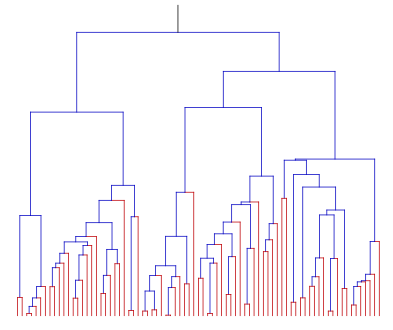
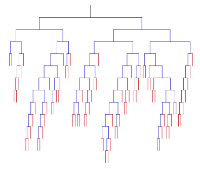
Figure 1. The effect of bias selection. Simulation of a binary ($p_{2}=1$ so $m=2$) age-dependent tree with $B$ given in Section 4, up to time $T=8$ ($|\mathcal{T}_{T}|=145$). Left: the size of each segment represents the lifetime of an individual. Individuals alive at time $T$ are represented in red. Right: genealogical representation of the same realisation of the tree.

Observation schemes

We assume we observe the whole trajectory $(X(t),t\in[0,T])$, where $T>0$ is a fixed (large) terminal time. Asymptotics are taken as $T\rightarrow\infty$. If we denote by $\mathcal{T}_{T}$ the population of individuals that are born before $T$ and observed up to time $T$ and if $(\zeta_{u}^{T},u\in\mathcal{T}_{T})$ denotes the values of the ages of the different individuals of $\mathcal{T}_{T}$ (at their time of death or at time $T$), we wish to draw inference on $B(x)$ based on

$$\big{\{}X(t),t\in[0,T]\big{\}}=\big{\{}\zeta_{u}^{T},u\in\mathcal{T}_{T}\big{\}}.$$

Although the lifetimes of the individuals are independent (and identically distributed) with common density $f$, this is no longer the case for the population $(\zeta_{u}^{T},u\in\mathcal{T}_{T})$ considered as a whole: the tree structure plays a crucial role and we have to face several non-trivial difficulties:

• Bias selection: particles with small lifetimes are more often observed than particles with large lifetimes since the observation of the process is stopped along all the branches at the fixed time $T$, as illustrated in Figure 1.

• Censoring: if $\partial\mathcal{T}_{T}\subset\mathcal{T}_{T}$ denotes the population of individuals alive at time $T$ (in red in Figure 1), they are censored in our observation scheme (we observe their lifetime only up to time $T$) but contribute to the whole estimation process at the same level as the population $\mathring{\mathcal{T}}_{T}\subset\mathcal{T}_{T}$ of individuals born and dead before $T$: due to the supercriticality of the process ($m>1$) we have $|\mathcal{T}_{T}|\approx|\mathring{\mathcal{T}}_{T}|\approx|\partial\mathcal{T}_{T}|$ as $T$ grows to infinity, and this affects the statistical analysis, see Section 2.2 below.

• Non-ancillarity: the number of observations $|\mathcal{T}_{T}|$ that governs the amount of statistical information is random and its distribution depends on $B$: we essentially have less observations if $B$ is small (particles split at a slow rate) than if $B$ is large (particles split at a fast rate). This means that $|\mathcal{T}_{T}|$ is not ancillary in the terminology of Fisher: it is not possible to ignore its randomness (by conditioning upon its value for instance) without losing some statistical information. We refer to the Encyclopedia of Statistics [17] for more details.

Main results

We first study in Section 2 the behaviour of empirical measures of the form

$$\mathcal{E}^{T}(\mathcal{V},g)=|\mathcal{V}|^{-1}\sum_{u\in\mathcal{V}}g(\zeta_{u}^{T}),\;\;\text{with}\;\;\mathcal{V}=\mathring{\mathcal{T}_{T}}\;\;\text{or}\;\;\partial\mathcal{T}_{T}$$

for suitable test functions $g$. From the classical study of critical branching processes, it is known that $|\mathring{\mathcal{T}_{T}}|\approx|\partial\mathcal{T}_{T}|\approx e^{\lambda_{B}T}$, where $\lambda_{B}>0$ is the Malthus parameter associated to the model (Harris [12] and (6) below). Both $\mathcal{E}^{T}(\mathring{\mathcal{T}_{T}},g)$ and $\mathcal{E}^{T}(\partial\mathcal{T}_{T},g)$ converge to their respective limits with rate $\exp(-\lambda_{B}T/2)$, with some uniformity in $B$ and $g$ as shown in Theorem 3 and 4 below. For the proof, we heavily rely on the recent studies of Cloez [5] and Bansaye et al. [3], two key references for this paper, adjusting the tools developed in [3] to the non-Markovian case: the essential ingredient is the use of many-to-one formulae that reduce the problem to studying the evolution of a particle picked at random along the genealogical tree (Propositions 10 and 11). The rate of convergence to equilibrium of this tagged particle, which governs the rates of convergence for statistical estimators, is obtained by a simple coupling argument (Proposition 12).

These preliminary results enable us to address the main issue of the paper: we construct in Section 3 a nonparametric estimator $\widehat{B}_{T}(x)$ of $B(x)$ that achieves the rate of convergence $\exp(-\lambda_{B}\frac{\beta}{2\beta+1}T)$ for pointwise error and uniformly over functions $B$ with local smoothness of order $\beta>0$ (Theorem 7). We show that this rate is optimal in a minimax sense in Theorem 8, thanks to statistical tools developed in Löcherbach [18]. This result is obtained under the restriction that convergence to equilibrium of a tagged particle is faster than the growth of the tree. Otherwise, we still have a rate of convergence, but we do not have (nor believe in) its optimality. We bypass the aforementioned bias selection difficulty 1) by weighting a kernel estimator by a de-biasing factor that depends on preliminary estimators of $\lambda_{B}$ and $m$. These estimators (essentially) converge with rate $\exp(-\lambda_{B}T/2)$ as shown in Proposition 5. As for the censoring part 2), we base our nonparametric kernel estimator on $\mathcal{E}^{T}(\mathring{\mathcal{T}_{T}},g)$ and not on $\mathcal{E}^{T}(\partial\mathcal{T}_{T},g)$, since that latter quantity would lead to a subobtimal rate of convergence as discussed in Section 3.3. Finally, the non-ancillarity issue 3) is solved by specifying a random bandwidth for the kernel that also depends on the preliminary estimation of $\lambda_{B}$. This last point requires extra efforts in order to show a form of stability that is detailed in Proposition 17.

The statistical study of branching processes goes back to Athreya and Keiding [1] for deriving maximum likelihood theory in the case of a parametric (constant) division rate, relying on the fact that the number of living cells is then a Markov process, a property we lose here for a non-constant division rate $x\leadsto B(x)$. The textbook of Guttorp [11] gives an account of existing parametric methods in the 1990’s. In the early 2000’s the regularity in the sense of the LAN and LAMN property was established in the comprehensive study of Löcherbach [18, 19], see also Hyrien [15] for statistical computational methods and Johnson et al. [16] for Bayesian analysis, and Delmas and Marsalle [6] in discrete time. In nonparametric estimation, only few results exist; we mention the case when dynamics between jumps is driven by a diffusion in Höpfner et al. [14]. To the best or our knowledge, our study provides with the first fully nonparametric approach in continuous time in supercritical branching processes which are piecewise deterministic. Admittedly, the Bellman-Harris model is a toy model for the study of population dynamics, but we believe that the present contribution sheds some light in the intrinsic difficulties that need to be solved in more elaborate models like cell equation for which only simplified statistical models have been considered so far (in discrete time or under additional deterministic or stochastic noise like in e.g. [9, 8, 7]). Concerning bias selection, density estimation when observing a biased sample has been studied at length framework by Efromovich [10].

Organisation of the paper

In Section 2, we define our rigorous statistical framework by means of continuous time rooted trees (Section 2.1) and study the convergence properties of the biased empirical measures $\mathcal{E}^{T}(\mathring{\mathcal{T}_{T}},g)$ and $\mathcal{E}^{T}(\partial\mathcal{T}_{T},g)$ in Section 2.3. We start by deriving heuristically the respective limits of the empirical measures in Section 2.2 (that can also be found in Cloez [5] and Bansaye et al. [3]) in order to shed some light on the specific methods of proof in the subsequent study of rate of convergence. We construct in Section 3 the estimators of $m$, $\lambda_{B}$ and $B(x)$ and state our statistical results together with a discussion on the extensions and limitations of our findings. Section 4 tackles the problem of numerical implementation on simulated data, advocating for a reasonably use of our estimators in practice. Section 5 is devoted to the proofs. An appendix (Section 6) contains auxiliary useful results.

2. Rate of convergence for biased empirical measures

2.1. Continuous time rooted trees

It will prove more convenient to work with a representation of $(X(t))_{t\geq 0}$ in terms of a continuous time rooted tree. We need some notation and closely follow Bansaye et al. [3]. Let

$$\mathcal{U}=\bigcup_{k\geq 0}(\mathbb{N}^{\star})^{k}$$

with $\mathbb{N}^{\star}=\{1,2,\ldots\}$ and $(\mathbb{N}^{\star})^{0}=\{\varnothing\}$ denote the infinite genealogical tree. We use throughout the following standard notation: for $u=(u_{1},u_{2},\ldots,u_{m})$ and $v=(v_{1},\ldots,v_{n})$ in $\mathcal{U}$, we write $uv=(u_{1},\ldots,u_{m},v_{1},\ldots,v_{n})$ for the concatenation, we identify $\varnothing u$, $u\varnothing$ and $u$, we write $u\preceq v$ if there exists $w$ such that $uw=v$ and $u\prec v$ if $u\preceq v$ and $w\neq\varnothing$. For $u=(u_{1},u_{2},\ldots,u_{m})$, we also write $|u|=m$.

Given a family $(\nu_{u},u\in\mathcal{U})$ of integers representing the number of children of the individuals $u\in\mathcal{U}$, we construct an ordered rooted tree $\mathcal{T}\subset\mathcal{U}$ as follows:

• $\varnothing\in\mathcal{T}$,

• If $v\in\mathcal{T}$, $u\preceq v$ implies $u\in\mathcal{T}$,

• For every $u\in\mathcal{T}$, we have $uj\in\mathcal{T}$ if and only if $1\leq j\leq\nu_{u}$.

For a family $(\zeta_{u},u\in\mathcal{U})$ of nonnegative numbers representing the lifetimes of the individuals $u\in\mathcal{U}$, we set

(4) $$b_{u}=\sum_{v\prec u}\zeta_{v}\;\;\text{and}\;\;d_{u}=b_{u}+\zeta_{u}$$

for the times of birth and death of the individual $u\in\mathcal{U}$. Let $\mathbb{U}=\mathcal{U}\times[0,\infty).$ A continuous time rooted tree is then a subset $\mathbb{T}$ of $\mathbb{U}$ such that

• $(\varnothing,0)\in\mathbb{T}$,

• The projection $\mathcal{T}$ of $\mathbb{T}$ on $\mathcal{U}$ is an ordered rooted tree,

• There exists a family $(\zeta_{u},u\in\mathcal{U})$ of nonnegative numbers such that $(u,s)\in\mathbb{T}$ if and only if $b_{u}\leq s<d_{u}$, where $(b_{u},d_{u})$ are defined by (4).

We now work on some probability space $(\Omega,\mathcal{F},\mathbb{P})$. In this setting, we have the following

Definition 1 (The Bellman-Harris model).

A random continuous time rooted tree is a Bellman-Harris model with offspring distribution $p=(p_{k})_{k\geq 1}$ and division rate $B:[0,\infty)\rightarrow[0,\infty)$ if

1. The family of the number of children $(\nu_{u},u\in\mathcal{U})$ are independent random variables with common distribution $p$.

2. The family of lifetimes $(\zeta_{u},u\in\mathcal{U})$ are independent random variables such that

   (5) $$\mathbb{P}\big{(}\zeta_{u}\geq x\big{)}=\exp\big{(}-\int_{0}^{x}B(y)dy\big{)},\;\;x\geq 0,$$

   with

   $$\int^{\infty}B(x)dx=\infty,$$

3. The families of random variables $(\nu_{u},u\in\mathcal{U})$ and $(\zeta_{u},u\in\mathcal{U})$ are independent.

Going back to the process $(X(t))_{t\geq 0}$ defined in (2),we have an identity between point measures on $(0,\infty)$ that reads

$$\sum_{i\geq 1}{\bf 1}_{\{X_{i}(t)>0\}}\delta_{X_{i}(t)}=\sum_{u\in\mathcal{T}}{\bf 1}_{\{t\in[b_{u},d_{u})\}}\delta_{t-b_{u}}.$$

The following assumption will be in force in the paper:

Assumption 2.

The offspring distribution $p=(p_{k})_{k\geq 0}$ satisfies

$$p_{0}=p_{1}=0,\;\;2\leq m=\sum_{k\geq 2}kp_{k}<\infty,\quad\sum_{k\geq 2}k^{2}p_{k}<\infty\;\;\text{and}\;\;\bar{m}=\sum_{i\neq j}\sum_{k\geq i\vee j}p_{k}<\infty.$$

The technical condition $\bar{m}<\infty$ is needed for the so-called many-to-one formulae, see Proposition 11 below.

2.2. The limiting objects

In order to extract information about $x\leadsto B(x)$, we consider the empirical distribution function over the lifetimes indexed by some $\mathcal{V}_{T}\subset\mathcal{T}_{T}$ for a test function $g$, that is

$$\mathcal{E}^{T}(\mathcal{V}_{T},g)=|\mathcal{V}_{T}|^{-1}\sum_{u\in\mathcal{V}_{T}}g(\zeta_{u}^{T}),$$

and expect a law of large number as $T\rightarrow\infty$. Without much of a surprise, it turns out that depending whether $\zeta_{u}^{T}=\zeta_{u}$ or not, i.e. if the data are still alive at time $T$, therefore censored or not, we have a different limit. More precisely, define

$$\mathring{\mathcal{T}}_{T}=\{u\in\mathcal{T},b_{u}<T\;\text{and}\;d_{u}\leq T\}\;\;\text{and}\;\;\partial\mathcal{T}_{T}=\{u\in\mathcal{T},b_{u}\leq T<d_{u}\},$$

i.e. the set of particles that are born and that die before $T$, and the set of particles alive at time $T$, so that $\mathcal{T}_{T}=\mathring{\mathcal{T}}_{T}\cup\partial\mathcal{T}_{T}.$ We need some notation. Introduce the Malthus parameter $\lambda_{B}>0$ defined as the (necessarily unique) solution to

(6) $$\int_{0}^{\infty}B(x)e^{-\lambda_{B}x-\int_{0}^{x}B(y)dy}dx=\frac{1}{m}.$$

To a division rate function $x\leadsto B(x)$ satisfying the properties of Definition 1, we associate its density lifetime

$$f_{B}(x)=B(x)\exp\big{(}-\int_{0}^{x}B(y)dy\big{)},\;x\geq 0$$

and its biased density lifetime

$$f_{H_{B}}(x)=me^{-\lambda_{B}x}f_{B}(x),\;x\geq 0,$$

which in turns uniquely defines a biased division rate

(7) $$H_{B}(x)=\frac{me^{-\lambda_{B}x}f_{B}(x)}{1-m\int_{0}^{x}e^{-\lambda_{B}y}f_{B}(y)ds}.$$

Finally, we define the limiting measures

(8) $$\partial\mathcal{E}_{B}(g)=\lambda_{B}\frac{m}{m-1}\int_{0}^{\infty}g(x)e^{-\lambda_{B}x}e^{-\int_{0}^{x}B(y)dy}dx$$

and

(9) $$\mathring{\mathcal{E}}_{B}\big{(}g\big{)}=m\int_{0}^{\infty}g(x)e^{-\lambda_{B}x}f_{B}(x)dx=\int_{0}^{\infty}g(x)f_{H_{B}}(x)dx.$$

It is known that $\mathcal{E}^{T}(\partial\mathcal{T}_{T},g)\rightarrow\partial\mathcal{E}_{B}(g)$ and $\mathcal{E}^{T}(\mathring{\mathcal{T}}_{T},g)\rightarrow\mathring{\mathcal{E}}_{B}\big{(}g\big{)}$ in probability as $T\rightarrow\infty$, see Appendix 6.1 for heuristics and references. We establish in Theorems 3 and 4 in the next Section 2.3 a rate of convergence with some uniformity in $B$. The rate is linked to $\lambda_{B}$ and the geometric ergodicity of an auxiliary one-dimensional Markov process with infinitesimal generator

(10) $$\mathcal{A}_{H_{B}}g(x)=g^{\prime}(x)+H_{B}(x)\big{(}g(0)-g(x)\big{)}$$

densely defined on continuous functions vanishing at infinity and that represents the value of a branch along the tree picked uniformly at random at each branching event.

2.3. Convergence results for biased empirical measures

Notation.

For constants $b,C>0$, introduce the sets

$$\mathcal{L}_{C}=\Big{\{}g:[0,\infty)\rightarrow{\mathbb{R}},\;\sup_{x}|g(x)|\leq C\Big{\}}$$

and

$$\mathcal{B}_{b,C}=\Big{\{}B:[0,\infty)\rightarrow[0,\infty),\forall x\geq 0:\;b\leq B(x)\leq b\max\{C,1\}\Big{\}}.$$

For a family $\Gamma_{T}=\big{(}\Gamma_{T}(\gamma)\big{)}_{T\geq 0}$ of real-valued random variables, with distribution depending on some parameter $\gamma\in\mathcal{G}$ we say that $\Gamma_{T}$ is $\mathcal{G}$-tight for the parameter $\gamma$ if

$$\sup_{T>0,\gamma\in\mathcal{G}}{\mathbb{P}}\big{(}|\Gamma_{T}(\gamma)|\geq K\big{)}\rightarrow 0\;\;\text{as}\;\;K\rightarrow\infty.$$

Results

We have a trade-off between the growth rate $\lambda_{B}$ of the tree $\mathbb{E}[|\mathcal{T}_{T}|]\approx e^{\lambda_{B}T}$ and the convergence to equilibrium of the Markov process with infinitesimal generator $\mathcal{A}_{H_{B}}$ defined in (10) above. More, precisely, we show in Proposition 12 below the estimate

$$\Big{|}P_{H_{B}}^{t}g(x)-\int_{0}^{\infty}g(y)\mu_{B}(y)dy\Big{|}\leq 2\sup_{y}|g(y)|e^{-\rho_{B}t}\;\;\text{for every}\;x\in(0,\infty).$$

Here, $(P_{H_{B}}^{t})_{t\geq 0}$ denotes the semigroup associated to $\mathcal{A}_{H_{B}}$ and $\mu_{B}$ its unique invariant probability, and

$$\rho_{B}=\inf_{x}H_{B}(x)$$

where $H_{B}(x)$ is the biased division rate defined in (7) above. The rate of convergence of the biased empirical measures $\mathcal{E}^{T}(\mathring{\mathcal{T}_{T}},g)$ and $\mathcal{E}^{T}(\partial\mathcal{T}_{T},g)$ to their limits $\partial{\mathcal{E}}_{B}(g)$ and $\mathring{\mathcal{E}}_{B}(g)$ respectively defined by (8) and (9) are goverened by $\lambda_{B}$ and $\rho_{B}$: define

(11) $$v_{T}(B)=\left\{\begin{array}[]{lll}e^{-\min\{\rho_{B},\lambda_{B}/2\}T}&\text{if}&\lambda_{B}\neq 2\rho_{B},\\ \\ T^{1/2}e^{-\lambda_{B}T/2}&\text{if}&\lambda_{B}=2\rho_{B}.\end{array}\right.$$

We have:

Theorem 3 (Rate of convergence for particles living at time $T$).

Work under Assumption 2. For every $b,C,C^{\prime}>0$,

$$v_{T}(B)^{-1}\big{(}\mathcal{E}^{T}\big{(}\partial{\mathcal{T}}_{T},g\big{)}-\partial{\mathcal{E}}_{B}(g)\big{)}$$

is $\mathbb{B}_{b,C}\times\mathcal{L}_{C^{\prime}}$-tight for the parameter $(B,g)$.

Theorem 4 (Rate of convergence for particles dying before $T$).

In the same setting as Theorem 3,

$$v_{T}(B)^{-1}\big{(}\mathcal{E}^{T}\big{(}\mathring{\mathcal{T}}_{T},g\big{)}-\mathring{\mathcal{E}}_{B}(g)\big{)}$$

is $\mathbb{B}_{b,C}\times\mathcal{L}_{C^{\prime}}$-tight for the parameter $(B,g)$.

Several comments are in order:

About the rate of convergence and the class $\mathcal{B}_{b,C}$:

the restriction $B\in\mathcal{B}_{b,C}$ enables us to obtain uniform convergence results. This is important for the subsequent statistical analysis. However, this can be relaxed if only $\mathcal{L}_{C^{\prime}}$-tightness is sought, provided $B$ complies to the conditions of Definition 1 and Assumption 2 and $\rho_{B}>0$. In the same direction, the rate $v_{T}(B)$ can be improved replacing $\rho_{B}=\inf_{x}H_{B}(x)$ in (11) by

(12) $$\rho_{B}^{\star}=\sup\Big{\{}\rho,\;\forall x,t>0:|P_{H_{B}}^{t}g(x)-\int_{0}^{\infty}g(y)\mu_{B}(y)dy|\leq 2\sup_{y}|g(y)|e^{-\rho t}\Big{\}},$$

and we have in particular $\rho_{B}^{\star}\geq\rho_{B}$.

About the tightness:

what we need in order to handle the random normalisation in $\mathcal{E}^{T}\big{(}\mathring{\mathcal{T}}_{T},g\big{)}$ is actually the convergence of $e^{\lambda_{B}T}|\mathring{\mathcal{T}}_{T}|^{-1}$. This convergence still holds in probability but not necessarily in $L^{2}({\mathbb{P}})$, so we only have tightness in Theorems 3 (and 4 for the same reason). However, if we replace $\mathcal{E}^{T}(\mathring{\mathcal{T}}_{T},g)$ by

$$\frac{1}{\mathbb{E}[|\mathring{\mathcal{T}}_{T}|]}\sum_{u\in\mathring{\mathcal{T}}_{T}}g(\zeta_{u}^{T}),$$

then we have a bound in $L^{2}({\mathbb{P}})$ together with a control on $g$, see Proposition 15 below. Such a finer control is mandatory for the subsequent statistical analysis, since we need to pick a function $g$ that depends on $T$ and that mimics the behaviour of the Dirac mass $\delta_{x}$, see Section 3 below.

3. Statistical estimation

3.1. Construction of an estimation procedure

Estimation of $m$ and $\lambda_{B}$

To a particle sitting at node $u\in\mathring{\mathcal{T}}_{T}$, we associate its number of children $\nu_{u}$ (see Definition 1). Note that the knowledge of ${\mathcal{T}}_{T}$ enables us to reconstruct $\nu_{u}$ for every $u\in\mathring{\mathcal{T}}_{T}$. This enables us to define an estimator for $m$ by setting

(13) $$\widehat{m}_{T}=|\mathring{\mathcal{T}}_{T}|^{-1}\sum_{u\in\mathring{\mathcal{T}}_{T}}\nu_{u}$$

on the set $|\mathring{\mathcal{T}}_{T}|\neq 0$ and $2$ otherwise. In order to estimate $\lambda_{B}$, we first observe that for $\mathrm{Id}(x)=x$, we can write

$$\mathring{\mathcal{E}}_{B}(\mathrm{Id}) =m\int_{0}^{\infty}x\big{(}B(x)+\lambda_{B}\big{)}e^{-\int_{0}^{x}(B(y)+\lambda_{B})dy}dx-m\lambda_{B}\int_{0}^{\infty}xe^{-\lambda_{B}x}e^{-\int_{0}^{x}B(y)dy}dx$$

$$=m\int_{0}^{\infty}e^{-\int_{0}^{x}(B(y)+\lambda_{B})dy}dx-m\lambda_{B}\tfrac{m-1}{m\lambda_{B}}\partial{\mathcal{E}}_{B}(\mathrm{Id})=m\tfrac{m-1}{m\lambda_{B}}-(m-1)\partial{\mathcal{E}}_{B}(\mathrm{Id}),$$

the last equality being obtained integrating by parts. So we obtain the following representation

$$\lambda_{B}=\Big{(}\tfrac{1}{m-1}\mathring{\mathcal{E}}_{B}(\mathrm{Id})+\partial{\mathcal{E}}_{B}(\mathrm{Id})\Big{)}^{-1}$$

and this yields the estimator

(14) $$\widehat{\lambda}_{T}=\Big{(}\tfrac{1}{\widehat{m}_{T}-1}|\mathring{\mathcal{T}}_{T}|^{-1}\sum_{u\in\mathring{\mathcal{T}}_{T}}\zeta_{u}+|\partial{\mathcal{T}}_{T}|^{-1}\sum_{u\in\partial{\mathcal{T}}_{T}}\zeta_{u}^{T}\Big{)}^{-1}.$$

The following convergence result for $\widehat{\lambda}_{T}$ is then a consequence of Theorems 3 and 4.

Proposition 5.

In the same setting as Theorem 3 with $v_{T}(B)$ given in (11) above, we have that

$$e^{\lambda_{B}T/2}\big{(}\widehat{m}_{T}-m\big{)}\;\;\text{and}\;\;T^{-1}v_{T}(B)^{-1}\big{(}\widehat{\lambda}_{T}-\lambda_{B}\big{)}$$

are $\mathcal{B}_{b,C}$-tight for the parameter $B$.

Reconstruction formula for $B(x)$

An estimator $\widehat{B}_{T}:[0,\infty)\rightarrow{\mathbb{R}}$ of $B$ is a random function

$$\widehat{B}_{T}(x)=\widehat{B}_{T}\big{(}x,(X(t))_{t\in[0,T]}),\;\;x\in[0,\infty)$$

that is measurable as a function of $(X(t))_{t\in[0,T]}$ but also as a function of $x$. By (3), we have

$$B(x)=\frac{f_{B}(x)}{1-\int_{0}^{x}f_{B}(y)dy}$$

and from the definition $\mathring{\mathcal{E}}_{B}\big{(}g\big{)}=m\int_{0}^{\infty}g(x)e^{-\lambda_{B}x}f_{B}(x)dx$ we obtain the formal reconstruction formula

(15) $$B(x)=\frac{\mathring{\mathcal{E}}_{B}\big{(}m^{-1}e^{\lambda_{B}\cdot}\delta_{x}(\cdot)\big{)}}{1-\mathring{\mathcal{E}}_{B}\big{(}m^{-1}e^{\lambda_{B}\cdot}{\bf 1}_{\{\cdot\leq x\}}\big{)}}$$

where $\delta_{x}(\cdot)$ denotes the Dirac function at $x$. Therefore, substituting $m$ and $\lambda_{B}$ by the estimators defined in (13) and (14) and taking $g$ as a weak approximation of $\delta_{x}$, we obtain a strategy for estimating $B(x)$ replacing furthermore $\mathring{\mathcal{E}}_{B}(\cdot)$ by its empirical version ${\mathcal{E}}^{T}(\mathring{\mathcal{T}}_{T},\cdot)$.

Construction of a kernel estimator and function spaces

Let $K:{\mathbb{R}}\rightarrow{\mathbb{R}}$ be a kernel function. For $h>0$, set $K_{h}(x)=h^{-1}K(h^{-1}x)$. In view of (15), we define the estimator

$$\widehat{B}_{T}(x) =\frac{{\mathcal{E}}^{T}\big{(}\mathring{\mathcal{T}}_{T},\widehat{m}_{T}^{-1}e^{\widehat{\lambda}_{T}\cdot}K_{h}(x-\cdot)\big{)}}{1-{\mathcal{E}}^{T}\big{(}\mathring{\mathcal{T}}_{T},\widehat{m}_{T}^{-1}e^{\widehat{\lambda}_{T}\cdot}{\bf 1}_{\{\cdot\leq x\}}\big{)}}$$

on the set ${\mathcal{E}}^{T}\big{(}\mathring{\mathcal{T}}_{T},\widehat{m}_{T}^{-1}e^{\widehat{\lambda}_{T}\cdot}{\bf 1}_{\{\cdot\leq x\}}\big{)}\neq 1$ and $0$ otherwise. Thus $\widehat{B}_{T}(x)$ is specified by the choice of the kernel $K$ and the bandwidth $h>0$. Note that the observations $(\zeta_{u},u\in\partial\mathcal{T}_{T})$ only occur in the estimator $\widehat{\lambda}_{T}$ of $\lambda_{B}$.

We need the following property on $K$:

Assumption 6.

The kernel $K:{\mathbb{R}}\rightarrow{\mathbb{R}}$ is differentiable with compact support and for some integer $n_{0}\geq 1$, we have $\int_{-\infty}^{\infty}x^{k}K(x)dx={\bf 1}_{\{k=0\}}$ for $k=1,\ldots,n_{0}$.

Assumption 6 will enable us to have nice approximation results over smooth functions $B$, described in the following way: for a compact interval $\mathcal{D}\subset(0,\infty)$ and $\beta>0$, with $\beta=\lfloor\beta\rfloor+\{\beta\}$, $0<\{\beta\}\leq 1$ and $\lfloor\beta\rfloor$ an integer, let $\mathcal{H}_{\mathcal{D}}^{\beta}$ denote the Hölder space of functions $g:{\mathcal{D}}\rightarrow{\mathbb{R}}$ possessing a derivative of order $\lfloor\beta\rfloor$ that satisfies

(16) $$|g^{\lfloor\beta\rfloor}(y)-g^{\lfloor\beta\rfloor}(x)|\leq c(g)|x-y|^{\{\beta\}}.$$

The minimal constant $c(g)$ such that (16) holds defines a semi-norm $|g|_{{\mathcal{H}}_{\mathcal{D}}^{\beta}}$. We equip the space ${\mathcal{H}}^{\beta}_{\mathcal{D}}$ with the norm $\|g\|_{{\mathcal{H}}^{\beta}_{\mathcal{D}}}=\sup_{x}|g(x)|+|g|_{{\mathcal{H}}_{\mathcal{D}}^{\beta}}$ and the balls

$${\mathcal{H}}_{\mathcal{D}}^{\beta}(L)=\{g:\mathcal{D}\rightarrow{\mathbb{R}},\;\|g\|_{{\mathcal{H}}_{\mathcal{D}}^{\beta}}\leq L\},\;L>0.$$

3.2. Convergence results for $\widehat{B}_{T}(x)$

We are ready to give our main result, namely a rate of convergence of $\widehat{B}_{T}(x)$ for $x$ restricted to a compact interval $\mathcal{D}$, uniformly over Hölder balls ${\mathcal{H}}_{\mathcal{D}}^{\beta}(L)$ of (known) smoothness $\beta$ intersected with $\mathcal{B}_{b,C}$. Define

(17) $$w_{T}(B)=T^{{\bf 1}_{\{\lambda_{B}=2\rho_{B}\}}}\exp\big{(}-\min\{\lambda_{B},2\rho_{B}\}\frac{\beta-(\lambda_{B}/\rho_{B}-1)_{+}/2}{2\beta+1}T\big{)}$$

and note that when $\rho_{B}\geq\lambda_{B}$, we have $w_{T}(B)=e^{-\lambda_{B}\frac{\beta}{2\beta+1}T}\approx\mathbb{E}[|\mathcal{T}_{T}|]^{-\beta/(2\beta+1)}$.

Theorem 7 (Upper rate of convergence).

Specify $\widehat{B}_{T}$ with a kernel satisfying Assumption 6 for some $n_{0}>1$ and

(18) $$h=\widehat{h}_{T}=\exp\big{(}-\widehat{\lambda}_{T}\tfrac{1}{2\beta+1}T\big{)}$$

for some $\beta\in[1/2,n_{0})$. For every $b,C>0,L>0$, every compact interval $\mathcal{D}$ in $(0,\infty)$ (with non-empty interior) and every $x\in\mathcal{D}$,

$$w_{T}(B)^{-1}\big{(}\widehat{B}_{T}(x)-B(x)\big{)}$$

is $\mathcal{B}_{b,C}\cap\mathcal{H}^{\beta}_{\mathcal{D}}(L)$-tight for the parameter $B$.

We have a partial optimality result in a minimax sense. Define

$$\mathcal{B}^{+}_{b,C}=\big{\{}B\in\mathcal{B}_{b,C},\;\lambda_{B}\leq\rho_{B}\big{\}}\;\;\text{and}\;\;\mathcal{B}^{-}_{b,C}=\big{\{}B\in\mathcal{B}_{b,C},\;\rho_{B}\leq\lambda_{B}\big{\}}$$

so that $\mathcal{B}_{b,c}=\mathcal{B}^{+}_{b,C}\cup\mathcal{B}^{-}_{b,C}$ We then have the following

Theorem 8 (Lower rate of convergence over $\mathcal{B}_{b,C}^{+}$).

Let $\mathcal{D}$ be a compact interval in $(0,\infty)$. For every $x\in\mathcal{D}$ and every positive $b,C,\beta,L$, there exists $C^{\prime}>0$ such that

$$\liminf_{T\rightarrow\infty}\inf_{\widehat{B}_{T}}\sup_{B}{\mathbb{P}}\big{(}e^{\lambda_{B}\frac{\beta}{2\beta+1}T}\big{|}\widehat{B}_{T}(x)-B(x)\big{|}\geq C^{\prime}\big{)}>0,$$

where the supremum is taken among all $B\in\mathcal{B}^{+}_{b,C}\cap\mathcal{H}^{\beta}_{\mathcal{D}}(L)$ and the infimum is taken among all estimators.

We observe a conflict between the rate growth of the tree $\lambda_{B}$ and its convergence rate to equilibrium $\rho_{B}$. On $\mathcal{B}^{+}_{b,C}$ we retrieve the expected usual optimal rate of convergence $\exp(-{\lambda_{B}\tfrac{\beta}{2\beta+1}T})\approx\mathbb{E}[|\mathcal{T}_{T}|]^{-\beta/(2\beta+1)}$ whereas if $\rho_{B}\leq\lambda_{B}$, we obtain the deteriorated rate $\exp\big{(}-\min\{\lambda_{B},2\rho_{B}\}(\beta-\tfrac{1}{2}(\tfrac{\lambda_{B}}{\rho_{B}}-1))/(2\beta+1)T\big{)}$ and this rate is presumably not optimal, as discussed at length in Section 3.3 below.

3.3. Discussion of the results

Rates of convergence

The “parametric case” for a constant division rate $B(x)=b$ with $b>0$ has a statistical simpler structure, but also a nice probabilistic feature since the process $t\leadsto|\partial\mathcal{T}_{t}|$, i.e. the number of cells alive at time $t$ is Markov. In that setting, explicit (asymptotic) information bounds are available (Athreya and Keiding [1]). In particular, the model is regular with asymptotic Fisher information of order $e^{\lambda_{B}T}$, thus the best-achievable (normalised) rate of convergence is $e^{-\lambda_{B}T/2}$. This is consistent with the minimax rate $\exp(-{\lambda_{B}\tfrac{\beta}{2\beta+1}T})$ that we obtain for the class $\mathcal{H}^{\beta}_{\mathcal{D}}(L)\cap\mathcal{B}_{b,C}^{+}$, and we retrieve the parametric rate by formally setting $\beta=\infty$ in the previous formula.

However, this rate is strongly parameter dependent in the sense that it also depends on $B$ via $\lambda_{B}$. This dependence is severe, since it appears at the same level as the smoothness exponent $\beta/(2\beta+1)$ in the rate exponent $\frac{\beta}{2\beta+1}\lambda_{B}$. For instance, in the simplest case of a constant function $B(x)=b$ for every $x\geq 0$, we have $\lambda_{B}=(m-1)b$, and we see that $B$ ($b$ here) plays at the same level as $\beta/(2\beta+1)$. This also has a non-trivial technical cost in establishing rates of convergence for the estimator $\widehat{B}_{T}(x)$: in order to minimise the bias-variance tradeoff, the (log)-bandwidth has to be chosen as $-\lambda_{B}\frac{1}{2\beta+1}T\big{(}1+o(1)\big{)}$ exactly, and this is achieved by the plug-in rule $-\widehat{\lambda}_{T}\frac{1}{2\beta+1}T$ thanks to Proposition 17. We then have to carefully check that our estimator is not too sensitive to this further approximation, and this requires the analysis of the smoothness of the process $h\leadsto\widehat{B}_{T,h}(x)$ where $h$ is the bandwidth of $\widehat{B}_{T}(x)$, as shown in Proposition 17.

Fast convergence to equilibrium in $\mathcal{B}_{b,C}^{+}$ versus slow convergence in $\mathcal{B}_{b,C}^{-}$

While we have an optimal rate of convergence over $\mathcal{B}_{b,B}^{+}$, the situation is unclear over $\mathcal{B}_{b,C}^{-}$. First, the convergence rate to equilibrium $\rho_{B}$ should be replaced by an estimator and that would lead to extraneous difficulties. Even if we knew $\rho_{B}$, optimising the bias-variance trade-off in the proof of Theorem 7 would not lead to the expected rate $\exp(-\min\{\lambda_{B},2\rho_{B}\}\tfrac{\beta}{2\beta+1}T)$ but to an intermediate rate that reads

(19) $$\exp\big{(}-\min\{\lambda_{B},2\rho_{B}\}\frac{\min\{\max\{\rho_{B}/\lambda_{B},1/2\},1\}\beta}{2\min\{\max\{\rho_{B}/\lambda_{B},1/2\},1\}\beta+1}T\big{)},$$

and that continuously deteriorates as $\rho_{B}$ separates $\lambda_{B}$ from below. Let us also mention that the classes $\mathcal{B}_{b,C}^{+}$ and $\mathcal{B}_{b,C}^{-}$ are never trivial. To that end, define

(20) $$\mathbb{B}_{b,m}=\big{\{}B\in\mathcal{B}_{b,m/(m-1)},\;\forall x\geq 0:B^{\prime}(x)-B(x)^{2}\leq 0\big{\}}$$

where $m=\sum_{k\geq 2}kp_{k}$ is the mean number of children at each branching event.

Proposition 9.

For any $b>0$, we have $\mathbb{B}_{b,m}\subset\mathcal{B}^{+}_{b,m/(m-1)}$. For every $C>2m(m+2)b/(m-1),\beta>0$ and any compact interval $\mathcal{D}\subset(0,\infty)$, there exists $B\in\mathcal{H}_{\mathcal{D}}^{\beta}$ such that $B\in\mathcal{B}_{b,C}^{-}$ and $B\notin\mathcal{B}_{b,C}^{+}$.

In the proof of Proposition 9 below we show a versatility in the choice of functions $B$ that yield either fast or slow rate of convergence to equilibrium. Finally, one could (at least formally) replace $\rho_{B}$ by $\rho_{B}^{\star}$, the optimal geometric rate of convergence to equilibrium defined in(12) above, but that would only improve on the rate of convergence (19) replacing $\rho_{B}$ by $\rho_{B}^{\star}$ which we do not know how to estimate, neither analytically nor statistically and the obtained result would still presumably not be optimal. This suggests a totally different estimation strategy – that we do not have at the moment – whenever convergence to equilibrium is slow.

Other loss functions

If $\mathcal{K}\subset\mathring{\mathcal{D}}$ is a closed interval ($\mathring{\mathcal{D}}$ denotes the interior of $\mathcal{D}$), then Theorem 7 also holds uniformly in $x\in\mathcal{K}$. So we also have that

$$w_{T}(B)^{-2}\int_{\mathcal{K}}(\widehat{B}_{T}(x)-B(x)\big{)}^{2}dx$$

is $\mathcal{B}_{b,C}\cap\mathcal{H}^{\beta}_{\mathcal{D}}(L)$-tight for the parameter $B$. For integrated squared error-loss, we could weaken the smoothness constraint $B\in{\mathcal{H}}_{\mathcal{D}}^{\beta}(L)$ to Sobolev smoothness (see e.g. [24]) when the smoothness is measured in $L^{2}$-norm. An extension of Theorem 8 can be obtained likewise.

Smoothness adaptation

Our estimator $\widehat{B}_{T}(x)$ is not $\beta$-adaptive, in the sense that the choice of the $\mathcal{B}_{b,C}^{+}$-optimal (log) bandwidth $-\widehat{\lambda}_{T}\frac{1}{2\beta+1}T$ still depends on $\beta$, which is unknown in principle. In the numerical implementation Section 4 below, we address this issue from a practical point of view. However, a theoretical result is still needed. The classical analysis of adaptive (or other) kernel methods à la Lepski for instance shows that this boils down to proving concentration inequalities of the type

(21) $${\mathbb{P}}\big{(}\big{|}\mathcal{E}^{T}\big{(}\mathring{\mathcal{T}}_{T},g_{h}\big{)}-\mathring{\mathcal{E}}_{B}(g_{h})\big{|}\geq e^{\lambda_{B}T/2}c(q,T)\big{)}\leq e^{-q\lambda_{B}T},\;\;q>0,$$

where, for $0<h^{-1}\leq e^{\lambda_{B}T}$, the test function $g_{h}$ has the form $g_{h}(y)=h^{-1/2}g\big{(}h^{-1}(x-y)\big{)}$ with $x\in\mathcal{D}$ and $g\in\mathcal{L}_{C}$. The threshold $c(q,T)$ should be of order $q\lambda_{B}T$ and would inflate the risk by a slow term (of order T). By a suitable choice of $q$, it would then be possible to obtain adaptation for $\beta$ in compact intervals. Concentration inequalities like (21) have been explored in [4] in discrete time. To the best of our knowledge, such inequalities are not yet available in continuous time and lie beyond the scope of the paper.

Information from $\mathring{\mathcal{T}}_{T}$ versus $\partial{\mathcal{T}}_{T}$

In the regime $B\in\mathcal{B}_{b,C}^{+}$, having

$$\partial\mathcal{E}_{B}(g)=\lambda_{B}\frac{m}{m-1}\int_{0}^{\infty}g(x)e^{-\lambda_{B}x}\exp\big{(}-\int_{0}^{x}B(y)dy\big{)}dx$$

and ignoring the fact that the constants $m$ and $\lambda_{B}$ are unknown (or rather knowing that they can be estimated at the superoptimal rate $e^{\lambda_{B}T/2}$), we can anticipate that by picking a suitable test function $g$ mimicking a delta function $g(x)\approx\delta_{x}$, the information about $B(x)$ can only be inferred through $\exp(-\int_{0}^{x}B(y)dy)$, which imposes to further take a derivative hence some ill-posedness.

We can briefly make all these arguments more precise (still in the regime $B\in\mathcal{B}_{b,C}^{+}$) : we assume that we have estimators of $\widehat{m}_{T}$ of $m$ and $\widehat{\lambda}_{T}$ of $\lambda_{B}$ (using the ones defined in (13) and (14) or by any other means) that converge with rate $T^{-1}e^{\lambda_{B}T/2}$ as in Proposition 5. Consider the quantity

$$\widehat{f}_{h,T}(x)=-\mathcal{E}^{T}\Big{(}\partial\mathcal{T}_{T},\frac{\widehat{m}_{T}-1}{\widehat{\lambda}_{T}\widehat{m}_{T}}\big{(}K_{h}\big{)}^{\prime}(x-\cdot)\Big{)}$$

for a kernel satisfying Assumption 6. By Theorem 3 and integrating by part, we readily see that

(22) $$\widehat{f}_{h,T}\rightarrow-\partial\mathcal{E}_{B}\Big{(}\frac{m-1}{\lambda_{B}m}\big{(}K_{h}\big{)}^{\prime}(x-\cdot)\Big{)}=\int_{0}^{\infty}K_{h}(x-y)f_{B+\lambda_{B}}(y)dy$$

in probability as $T\rightarrow\infty$, where $f_{B+\lambda_{B}}$ is the density associate to the division rate $x\leadsto B(x)+\lambda_{B}$. On the one hand, it is not difficult to show that Proposition 15 (used in the proof of Theorem 7 below) is valid when substituting $\mathring{\mathcal{T}}_{T}$ by $\partial\mathcal{T}_{T}$, so we expect (altough not formally established) the rate of convergence in (22) to be of order $h^{-3/2}e^{\lambda_{B}T/2}$ since we take the derivative of the kernel $K_{h}$. On the other hand, the limit $\int_{0}^{\infty}K_{h}(x-y)f_{B+\lambda_{B}}(y)dy$ approximates $f_{B+\lambda_{B}}(x)$ with an error of order $h^{\beta}$ if $B\in\mathcal{H}^{\beta}_{\mathcal{D}}.$ Balancing the two error terms in $h$, we see that we can estimate $f_{B+\lambda_{B}}(x)$ with an error of (presumably optimal) order $\exp(-\lambda_{B}\tfrac{\beta}{2\beta+3}T)$. Due to the fact that the denominator in representation (3) can be estimated with parametric error rate $\exp(-\lambda_{B}T/2)$ (possibly up to polynomially slow terms in $T$), we end up with the rate of estimation $\exp(-\lambda_{B}\frac{\beta}{2\beta+3}T)$ for $B(x)$ as well, and that can be related to an ill-posed problem of order 1 (see for instance [24]).

This phenomenon, namely the structure of an ill-posed problem of order 1 in restriction to data alive at time $T$, has already been observed in other settings: for the estimation of a size-division rate from living cells at a given large time in Doumic et al. [9, 8] or for the estimation of the dislocation measure for a homogeneous fragmentation in Hoffmann and Krell [13]. Note also that this phenomenon does not appear in parametric estimation, since the number of data in $\mathring{\mathcal{T}}_{T}$ and $\partial\mathcal{T}_{T}$ are of the same order of magnitude (or put differently, the rates in Theorems 3 and 4 are the same and govern the rate of estimation of a one dimensional parameter).

4. Numerical implementation

We assume that each cell $u\in\mathcal{U}$ has exactly two children at each division ($p_{2}=1$). This can model the evolution of a population of cells reproducing by binary divisions, as described deterministically by (1). We pick a trial division rate $B$ defined analytically by

$$B(x)=\left\{\begin{array}[]{lll}\tfrac{1}{3}x^{3}-\tfrac{7}{8}x^{2}+\tfrac{5}{8}x+\tfrac{4}{10}&\text{if}&0\leq x\leq\tfrac{3}{2}\\ \\ \tfrac{119}{160}-\tfrac{1}{4}\exp\big{(}-(x-\tfrac{3}{2})\big{)}&\text{if}&x>\tfrac{3}{2}\end{array}\right.$$

and represented in Figure 2 (bold red line). We have $b\leq B(x)\leq\tfrac{m}{m-1}b$ for any $x\geq 0$ for $b=0.4$ and $m=2$ and the lifetime density $f_{B}$ is non increasing (except in a vicinity of zero). Given $T>0$ we simulate the lifetime of the rooted cell $\zeta_{\emptyset}$ with probability density $f_{B}$ and set $d_{\emptyset}=\zeta_{\emptyset}$. For $u\in\mathcal{U}$ such that $d_{u}>T$, we do not simulate the lifetimes of its descendants since they are not in the observation scheme $\mathring{\mathcal{T}}_{T}\cup\partial\mathcal{T}_{T}$. For $u\in\mathcal{U}$ such that $d_{u}\leq T$ we simulate $\zeta_{u0}$ and $\zeta_{u1}$ independently with probability density $f_{B}$; we set $d_{u0}:=d_{u}+\zeta_{u0}$ and $d_{u1}:=d_{u}+\zeta_{u1}$. Using R software, we generate $M=100$ trees up to time $T=23$, so that the mean number of observations $|\mathring{\mathcal{T}}_{T}|$ is sufficiently large. (Note that for a binary tree, we always have the identity $|\partial\mathcal{T}_{T}|=|\mathring{\mathcal{T}}_{T}|+1$.) Figure 1 represents a typical observation scheme with continuous or discrete representation. The (random) number of observations fluctuates a lot as shown in Table 1 where some elementary statistics are given.

Min.	1st Qu.	Med.	Mean	3rd Qu.	Max.	Std.
3 726	43 930	96 480	115 760	144 100	561 200	102 408

Table 1. Fluctuations of the number of observations $|\mathring{\mathcal{T}}_{T}|$ for $M=100$ Monte-Carlo continuous trees observed up to time $T=23$.

We take a Gaussian kernel $K(x)=(2\pi)^{-1/2}\exp(-x^{2}/2)$ and the bandwidth $\widehat{h}_{T}$ is chosen here according to the rule-of-thumb $1.06\hat{\sigma}|\mathring{\mathcal{T}_{T}}|^{-1/5}$ where $\hat{\sigma}$ is the empirical standard deviation of $(\zeta_{u},u\in\mathring{\mathcal{T}_{T}})$. We also implemented standard cross-validation with less success. We evaluate $\widehat{B}_{T}$ on a regular grid of $\mathcal{D}=[0.25,0.5]$ with mesh $\Delta x=0.01$. For each sample we compute the empirical error

$$e_{i}=\frac{\|\widehat{B}^{(i)}_{T}-B\|_{\Delta x}}{\|B\|_{\Delta x}},\quad i=1,\ldots,M,$$

where $\|\cdot\|_{\Delta x}$ denotes the discrete norm over the numerical sampling. Table 2 displays the mean-empirical error $\overline{e}=M^{-1}\sum_{i=1}^{M}e_{i}$ together with the empirical standard deviation $\big{(}M^{-1}\sum_{i=1}^{M}(e_{i}-\overline{e})^{2}\big{)}^{1/2}$.

$\boldsymbol{T}$	$13$	$15$	$17$	$19$	$21$	$23$
Mean $\boldsymbol{|\mathring{\mathcal{T}}_{T}|}$	652	1 847	5 202	14 634	41 151	115 760
$\boldsymbol{\overline{e}}$	0.1624	0.1046	0.0735	0.0448	0.0307	0.0178
Std. dev.	0.1052	0.0764	0.0599	0.0260	0.0197	0.0092

Table 2. Mean empirical relative error $\overline{e}$ and its standard deviation, with respect to $T$, for the division rate $B$ reconstructed over the interval $\mathcal{D}=[0.25,2.5]$ by the estimator $\widehat{B}_{T}$.

The comparison of the density of interest $f_{B}$ and the biased density $f_{H_{B}}$ on Figure 2 highlights the bias selection since $f_{H_{B}}$ gives more weight to small lifetimes than $f_{B}$. The error deteriorates as $x$ grows since the biased density $f_{H_{B}}$ (bold blue line - we approximate the Malthus parameter using (6) and we find $\lambda_{B}\approx 0.5173$) decreases, see Figure 2. The larger $T$, the better the reconstruction at a visual level, as shown on Figure 2 where $95\%$-level confidence bands are built so that for each point $x$, the lower and upper bounds include $95\%$ of the estimators $(\widehat{B}_{T}^{(i)}(x),i=1\ldots M)$. Close to $0$, $B(x)$ does not lie in the confidence band: our estimator exhibits a large bias there, and this is presumably due to a boundary effect. The error is close to $\exp(-2\lambda_{B}T/5)$ as expected: indeed, for a kernel of order $n_{0}$, the bias term in density estimation is of order $h^{\beta\wedge(n_{0}+1)}$. Given that $B$ is smooth in our example, we rather expect $\exp(-\lambda_{B}\frac{(n_{0}+1)}{2(n_{0}+1)+1}T)=\exp(-2\lambda_{B}T/5)$ for the Gaussian kernel with $n_{0}=1$ that we use here, and this is consistent with what we observe in Figure 3.

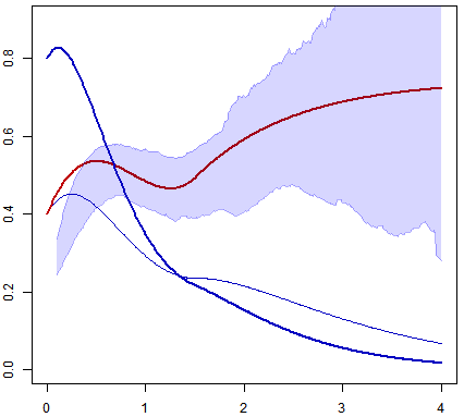
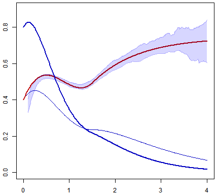
Figure 2. Reconstruction of $B$ over $\mathcal{D}=[0.1,4]$ with $95\%$-level confidence bands constructed over $M=100$ Monte-Carlo continuous trees. In bold red line: $x\leadsto B(x)$; in bold blue line: $f_{H_{B}}$; in blue line: $f_{B}$ (on the same $y$-axis scale). Left: $T=15$. Right: $T=23$.

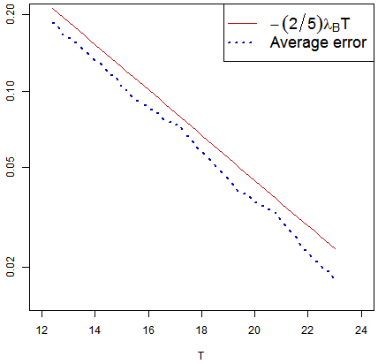
Figure 3. The log-average relative empirical error over $M=100$ Monte-Carlo continuous trees vs. $T$ (i.e. the log-rate) for $x\leadsto B(x)$ reconstructed over $\mathcal{D}=[0.25,2.5]$ with $x\leadsto\widehat{B}_{T}(x)$ (dashed blue line) compared to the expected log-rate (solid red line).

5. Proofs

For a locally integrable $B:[0,\infty)\rightarrow[0,\infty)$ such that $\int^{\infty}B(y)dy=\infty$, recall that we set

$$f_{B}(x)=B(x)e^{-\int_{0}^{x}B(y)dy},\;\;x\geq 0.$$

Recall that $H_{B}$ is characterised by

$$f_{H_{B}}(x)=me^{-\lambda_{B}x}f_{B}(x),\;\;x\geq 0.$$

5.1. Preliminaries

Many-to-one formulae

For $u\in\mathcal{U}$, we write $\zeta_{u}^{t}$ for the age of the cell $u$ at time $t\in I_{u}=[b_{u},d_{u})$, i.e. $\zeta_{u}^{t}=(t-b_{u}){\bf 1}_{\{t\in I_{u}\}}$. We extend $\zeta_{u}^{t}$ over $[0,b_{u})$ by setting $\zeta_{u}^{t}=\zeta_{u(t)}^{t}$, where $u(t)$ is the ancestor of $u$ living at time $t$, defined by $u(t)=v$ if $v\preceq u$ and $(v,t)\in\mathbb{T}$. For $t\geq d_{u}$ we set $\zeta_{u}^{t}=\zeta_{u}$. Note that $\zeta_{u}^{T}=\zeta_{u}$ on the event $u\in\mathring{\mathcal{T}}_{T}$.

Let $(\chi_{t})_{t\geq 0}$ and $(\widetilde{\chi}_{t})_{t\geq 0}$ denote the one-dimensional Markov processes with infinitesimal generators (densely defined on continuous functions vanishing at infinity) $\mathcal{A}_{B}$ and $\mathcal{A}_{H_{B}}$ respectively, where

$$\mathcal{A}_{B}g(x)=g^{\prime}(x)+B(x)\big{(}g(0)-g(x)\big{)}$$

and such that ${\mathbb{P}}(\chi_{0}=0)={\mathbb{P}}(\widetilde{\chi}_{0}=0)=1$. We also denote by $(P_{H_{B}}^{t})_{t\geq 0}$ the Markov semigroup associated to $\mathcal{A}_{H_{B}}$.

Proposition 10 (Many-to-one formulae).

For any $g\in\mathcal{L}_{C}$, we have

(23) $$\mathbb{E}\Big{[}\sum_{u\in\partial{\mathcal{T}}_{T}}g(\zeta_{u}^{T})\Big{]}=\frac{e^{\lambda_{B}T}}{m}\mathbb{E}\Big{[}g(\widetilde{\chi}_{T})B(\widetilde{\chi}_{T})^{-1}H_{B}(\widetilde{\chi}_{T})\Big{]},$$

and

(24) $$\mathbb{E}\Big{[}\sum_{u\in\mathring{\mathcal{T}}_{T}}g(\zeta_{u}^{T})\Big{]}=\mathbb{E}\Big{[}\sum_{u\in\mathring{\mathcal{T}}_{T}}g(\zeta_{u})\Big{]}=\frac{1}{m}\int_{0}^{T}e^{\lambda_{B}s}\mathbb{E}\Big{[}g(\widetilde{\chi}_{s})H_{B}(\widetilde{\chi}_{s})\Big{]}ds.$$

In order to compute rates of convergence, we will also need many-to-one formulae over pairs of individuals. We can pick two individuals in the same lineage or over forks, i.e. over pairs of individuals that are not in the same lineage. If $u,v\in\mathcal{U}$, $u\wedge v$ denote their most recent common ancestor. Define

$$\mathcal{FU}=\{(u,v)\in\mathcal{U}^{2},|u\wedge v|<|u|\wedge|v|\}\;\;\text{and}\;\;\mathcal{FT}=\mathcal{FU}\cap{\mathcal{T}}^{2}.$$

Introduce also $\bar{m}=\sum_{i\neq j}\sum_{k\geq i\vee j}p_{k}$ which is finite by Assumption 2.

Proposition 11 (Many-to-one formulae over pairs).

For any $g\in\mathcal{L}_{C}$, we have

(25) $$\mathbb{E}\Big{[}\sum_{u,v\in\partial{\mathcal{T}}_{T},\atop u\neq v}g(\zeta_{u}^{T})g(\zeta_{v}^{T})\Big{]}=\frac{\bar{m}}{m^{3}}\int_{0}^{T}e^{\lambda_{B}s}\Big{(}e^{\lambda_{B}(T-s)}P^{T-s}_{H_{B}}\big{(}g\frac{H_{B}}{B}\big{)}(0)\Big{)}^{2}P^{s}_{H_{B}}H_{B}(0)ds,$$

(26) $$\mathbb{E}\Big{[}\sum_{(u,v)\in\mathcal{FT}\cap\mathring{\mathcal{T}}_{T}^{2}}g(\zeta_{u})g(\zeta_{v})\Big{]}=\frac{\bar{m}}{m^{3}}\int_{0}^{T}e^{\lambda_{B}s}\bigg{(}\int_{0}^{T-s}e^{\lambda_{B}t}P_{H_{B}}^{t}(gH_{B})(0)dt\bigg{)}^{2}P_{H_{B}}^{s}H_{B}(0)ds,$$

and

(27) $$\mathbb{E}\big{[}\sum_{u,v\in\mathring{\mathcal{T}}_{T},\atop u\prec v}g(\zeta_{u})g(\zeta_{v})\big{]}=\int_{0}^{T}e^{\lambda_{B}s}\Big{(}\int_{0}^{T-s}e^{\lambda_{B}t}P^{t}_{H_{B}}\big{(}gH_{B}\big{)}(0)dt\Big{)}P^{s}_{H_{B}}(gH_{B})(0)ds.$$

The identity (25) is a particular case of Lemma 3.9 of Cloez [5]. In order to obtain identity (26), we closely follow the method of Bansaye et al. [3]. Although the setting in [3] is much more general than ours, it formally only applies for exponential renewal times (corresponding to constant functions $B$) so we need to slightly accommodate their proof. The same ideas enable us to prove (27). This is set out in details in the appendix.

Geometric ergodicity of the auxiliary Markov process

Define the probability measure

$$\mu_{B}(x)dx=c_{B}\exp(-\int_{0}^{x}H_{B}(y)dy)dx\;\;\text{for}\;\;x\geq 0.$$

We have the fast convergence of $P_{H_{B}}^{T}$ toward $\mu_{B}$ as $T\rightarrow\infty$. More precisely,

Proposition 12.

Let $\rho_{B}=\inf_{x}H_{B}(x)$. For any $B\in\mathcal{B}_{b,C}$, $g\in\mathcal{L}_{C^{\prime}}$, $t\geq 0$ and $x\in(0,\infty)$, we have

$$\Big{|}P_{H_{B}}^{t}g(x)-\int_{0}^{\infty}g(y)\mu_{B}(y)dy\Big{|}\leq 2\sup_{y}|g(y)|\exp\big{(}-\rho_{B}t\big{)}.$$

Proof.

First, one readily checks that $\int_{0}^{\infty}\mathcal{A}_{H_{B}}f(x)\mu_{B}(x)dx=0$ for any continuous $f$, and since moreover $P^{t}_{H_{B}}$ is Feller, it admits $\mu_{B}(x)dx$ as an invariant probability. It is now sufficient to show

$$\|Q_{B}^{x,t}-\mu_{B}\|_{TV}\leq\exp(-\rho_{B}t)$$

where $Q_{B}^{x,t}$ denotes the law of of the Markov process with infinitesimal generator $\mathcal{A}_{H_{B}}$ started from $x$ at time $t=0$ and $\|\cdot\|_{TV}$ is the total variation norm between probability measures. Let $N(ds\,dt)$ be a Poisson random measure with intensity $ds\otimes dt$ on $[0,\infty)\times[0,\infty)$. Define on the same probability space two random processes $(Y_{t})_{t\geq 0}$ and $(Z_{t})_{t\geq 0}$ such that

$$Y_{t} =x+t-\int_{0}^{t}\int_{0}^{\infty}Y_{s_{-}}{\bf 1}_{\{z\leq H_{B}(Y_{s^{-}})\}}N(dz\,ds),\;\;t\geq 0,$$

$$Z_{t} =Z_{0}+t-\int_{0}^{t}\int_{0}^{\infty}Z_{s_{-}}{\bf 1}_{\{z\leq H_{B}(Z_{s^{-}})\}}N(dz\,ds),\;\;t\geq 0,$$

where $Z_{0}$ is a random variable with distribution $\mu_{B}$. We have that both $(Y_{t})_{t\geq 0}$ and $(Z_{t})_{t\geq 0}$ are Markov processes driven by the same Poisson random measure with generator $\mathcal{A}_{H_{B}}$. Moreover, if $N$ has a jump in $[0,t)\times[0,\inf_{x}H_{B}(x)]$, then $Y_{t}$ and $Z_{t}$ both necessarily start from $0$ after this jump and coincide further on. It follows that

$${\mathbb{P}}(Y_{t}\neq Z_{t})\leq{\mathbb{P}}\Big{(}\int_{0}^{t}\int_{0}^{\inf_{x}H_{B}(x)}N(ds\,dt)=0\Big{)}=\exp(-\inf_{x}H_{B}(x)t)=\exp(-\rho_{B}t).$$

Observing that $Y_{t}$ and $Z_{t}$ have distribution $Q_{B}^{x,t}$ and $\mu_{B}$ respectively, we conclude thanks to the fact that $\|Q_{B}^{x,t}-\mu_{B}\|_{TV}\leq{\mathbb{P}}(Y_{t}\neq Z_{t})$.

∎

5.2. Proof of Theorems 3 and 4

In order to ease notation, when no confusion is possible, we abbreviate $\mathcal{B}_{b,C}$ by $\mathcal{B}$ and $\mathcal{L}_{C}$ by $\mathcal{L}$.

Proof of Theorem 3.

Writing

$$e^{\min\{\lambda_{B}/2,\rho_{B}\}T}\big{(}\mathcal{E}^{T}(\partial\mathcal{T}_{T},g)-\partial\mathcal{E}_{B}(g)\big{)}=\frac{e^{\lambda_{B}T}}{\big{|}\partial{\mathcal{T}}_{T}\big{|}}\,e^{(\min\{\lambda_{B}/2,\rho_{B}\}-\lambda_{B})T}\sum_{u\in\partial{\mathcal{T}}_{T}}\big{(}g(\zeta_{u}^{T})-\partial\mathcal{E}_{B}(g)\big{)},$$

Theorem 3 is then a consequence of the following two facts: first we claim that

(28) $$e^{\lambda_{B}T}\big{|}\partial{\mathcal{T}}_{T}\big{|}^{-1}\rightarrow W_{B}\;\;\text{in probability as}\;\;T\rightarrow\infty,$$

uniformly in $B\in\mathcal{B}$, where the random variable $W_{B}$ satisfies ${\mathbb{P}}(W_{B}>0)=1$, and second, for $B\in\mathcal{B}$ and $g\in\mathcal{L}$, we claim that the following estimate holds:

(29) $$\mathbb{E}\Big{[}\Big{(}\sum_{u\in\partial{\mathcal{T}}_{T}}\big{(}g(\zeta_{u}^{T})-\partial\mathcal{E}_{B}(g)\big{)}\Big{)}^{2}\Big{]}\lesssim e^{(2\lambda_{B}-\min\{\lambda_{B},2\rho_{B}\})T},$$

where $\lesssim$ means up to a constant (possibly varying from line to line) that only depends on $\mathcal{B}$ and $\mathcal{L}$ and up to a multiplicative slow term of order $T$ in the case $\lambda_{B}=2\rho_{B}$.

Step 1. The convergence (28) is a consequence of the following lemma:

Lemma 13.

For every $B\in\mathcal{B}$, there exists $\widetilde{W}_{B}$ with ${\mathbb{P}}(\widetilde{W}_{B}>0)=1$ such that

(30) $$\mathbb{E}\Big{[}\Big{(}\frac{|\partial{\mathcal{T}}_{T}|}{\mathbb{E}\big{[}|\partial{\mathcal{T}}_{T}|\big{]}}-\widetilde{W}_{B}\Big{)}^{2}\Big{]}\rightarrow 0\;\;\text{as}\;\;T\rightarrow\infty,$$

uniformly in $B\in\mathcal{B}$ and

(31) $$\kappa_{B}^{-1}e^{\lambda_{B}T}\mathbb{E}\big{[}|\partial{\mathcal{T}}_{T}|\big{]}\rightarrow 1\;\;\text{as}\;\;T\rightarrow\infty,$$

uniformly in $B\in\mathcal{B}$, where $\kappa_{B}^{-1}=\lambda_{B}\tfrac{m}{m-1}\int_{0}^{\infty}\exp(-\int_{0}^{x}H_{B}(y)dy)dx$.

Lemma 13 is well known, and follows from classical renewal arguments, see Chapter 6 in the book of Harris [12]. Only the uniformity in $B\in\mathcal{B}$ requires an extra argument, but with a uniform version of the key renewal theorem of [23], it readily follows from the proof of Harris, so we omit it. Note that (30) and (31) entail the convergence $e^{\lambda_{B}T}|\partial{\mathcal{T}}_{T}|^{-1}\rightarrow\kappa_{B}\widetilde{W}_{B}^{-1}=W_{B}$ in probability as $T\rightarrow\infty$ uniformly in $B\in\mathcal{B}$, and this entails (28).

Step 2. We now turn to the proof of (29). Without loss of generality, we may (and will) assume that $\partial\mathcal{E}_{B}(g)=0$. We have

$$\mathbb{E}\big{[}\big{(}\sum_{u\in\partial{\mathcal{T}}_{T}}g(\zeta_{u}^{T})\big{)}^{2}\big{]}=\mathbb{E}\big{[}\sum_{u\in\partial{\mathcal{T}}_{T}}g(\zeta_{u}^{T})^{2}\big{]}+\mathbb{E}\big{[}\sum_{u,v\in\partial{\mathcal{T}}_{T},\atop u\neq v}g(\zeta_{u}^{T})g(\zeta_{v}^{T})\big{]}=I+II,$$

say. By (23) in Proposition 10, we write

$$I =\frac{e^{\lambda_{B}T}}{m}\mathbb{E}\Big{[}g(\widetilde{\chi}_{T})^{2}B(\widetilde{\chi}_{T})^{-1}H_{B}(\widetilde{\chi}_{T})\Big{]}$$

$$\leq\frac{e^{\lambda_{B}T}}{m}\int_{0}^{\infty}g(x)^{2}\tfrac{H_{B}(x)}{B(x)}\mu_{B}(x)dx+\tfrac{e^{\lambda_{B}T}}{m}\Big{|}P^{T}_{H_{B}}\big{(}g^{2}\tfrac{H_{B}}{B}\big{)}(0)-\int_{0}^{\infty}g(x)^{2}\tfrac{H_{B}(x)}{B(x)}\mu_{B}(x)dx\Big{|}.$$

Since $g\in\mathcal{L}$ and $B\in\mathcal{B}$, we successively have

$$m^{-1}\int_{0}^{\infty}g(x)^{2}\tfrac{H_{B}(x)}{B(x)}\mu_{B}(x)dx\lesssim 1\;\;\text{and}\;\;g(x)^{2}\tfrac{H_{B}(x)}{B(x)}\lesssim 1.$$

Note that for $B\in\mathcal{B}$, we have

$$H_{B}(x)=\frac{B(x)}{\int_{x}^{\infty}B(y)e^{-\lambda_{B}(y-x)}\exp(-\int_{x}^{y}B(u)du)dy}\leq\frac{b^{2}\max\{C,1\}}{\lambda_{B}+b\max\{C,1\}}.$$

We also have $\lambda_{B}\leq\lambda_{\widetilde{B}}$ as soon as $B(x)\leq\widetilde{B}(x)$ for all $x$ (see for instance the proof of Proposition 9) so $\inf_{B\in\mathcal{B}}\lambda_{B}>0$ and the uniformity in the above estimates follows likewise. Applying Proposition 12 we derive

$$\Big{|}P^{T}_{H_{B}}\big{(}g^{2}\tfrac{H_{B}}{B}\big{)}(0)-\int_{0}^{\infty}g(x)^{2}\tfrac{H_{B}(x)}{B(x)}\mu_{B}(x)dx\Big{|}\lesssim 1,$$

and we conclude that $I\lesssim e^{\lambda_{B}T}\leq e^{(2\lambda_{B}-\min\{\lambda_{B},2\rho_{B}\})T}$. By (25) of Proposition 11 we have

$$II=\frac{\bar{m}e^{2\lambda_{B}T}}{m^{3}}\int_{0}^{T}e^{-\lambda_{B}s}\Big{(}P^{T-s}_{H_{B}}\big{(}g\tfrac{H_{B}}{B}\big{)}(0)\Big{)}^{2}P^{s}_{H_{B}}H_{B}(0)ds.$$

Since $B\in\mathcal{B}$ and $g\in\mathcal{L}$, the estimates $P^{s}_{H_{B}}H_{B}(0)\lesssim 1$ and $|g(x)|\tfrac{H_{B}(x)}{B(x)}\lesssim 1$ hold true. Applying Proposition 12 to the test function $g(x)\tfrac{H_{B}(x)}{B(x)}$ which has vanishing integral under $\mu_{B}$, we obtain

$$\big{|}P^{T-s}_{H_{B}}\big{(}g\tfrac{H_{B}}{B}\big{)}(0)\big{|}\lesssim e^{-\rho_{B}(T-s)}$$

hence

$$|II| \lesssim e^{2\lambda_{B}T}\int_{0}^{T}e^{-\lambda_{B}s}e^{-2\rho_{B}(T-s)}ds\lesssim\left\{\begin{array}[]{lll}e^{\lambda_{B}T}&\text{if}&2\rho_{B}\geq\lambda_{B}\\ e^{2(\lambda_{B}-\rho_{B})T}&\text{if}&2\rho_{B}<\lambda_{B},\end{array}\right.$$

up to a multiplicative slow term of order $T$ when $2\rho_{B}=\lambda_{B}$. Note also that the estimate is uniform in $B\in\mathcal{B}$ since $\inf_{B\in\mathcal{B}}\lambda_{B}>0$ and $\inf_{B\in\mathcal{B}}\rho_{B}>0$. We conclude $|II|\lesssim e^{(2\lambda_{B}-\min\{\lambda_{B},2\rho_{B}\})T}$. ∎

Proof of Theorem 4.

The proof goes along the same line but is slightly more intricate. First, we implicitly work on the event $\{\big{|}\mathring{\mathcal{T}}_{T}\big{|}\geq 1\}$ which has probability that goes to $1$ as $T\rightarrow\infty$, uniformly in $B\in\mathcal{B}$. We again write

$$e^{\min\{\lambda_{B}/2,\rho_{B}\}T}\big{(}\mathcal{E}(\mathring{\mathcal{T}_{T}},g)-\mathring{\mathcal{E}}_{B}(g)\big{)}=\frac{e^{\lambda_{B}T}}{\big{|}\mathring{\mathcal{T}}_{T}\big{|}}e^{(\min\{\lambda_{B}/2,\rho_{B}\}-\lambda_{B})T}\sum_{u\in\mathring{\mathcal{T}}_{T}}\big{(}g(\zeta_{u}^{T})-\mathring{\mathcal{E}}_{B}(g)\big{)},$$

and we claim that

(32) $$e^{\lambda_{B}T}\big{|}\mathring{\mathcal{T}}_{T}\big{|}^{-1}\rightarrow W_{B}^{\prime}>0\;\;\text{in probability as}\;\;T\rightarrow\infty,$$

uniformly in $B\in\mathcal{B}$, where $W_{B}^{\prime}$ satisfies ${\mathbb{P}}(W_{B}^{\prime}>0)=1$ and that the following estimate holds:

(33) $$\mathbb{E}\Big{[}\Big{(}\sum_{u\in\mathring{\mathcal{T}}_{T}}\big{(}g(\zeta_{u}^{T})-\mathring{\mathcal{E}}_{B}(g)\big{)}\Big{)}^{2}\Big{]}\lesssim e^{(2\lambda_{B}-\min\{\lambda_{B},2\rho_{B}\})T},$$

uniformly in $B\in\mathcal{B}$ and $g\in\mathcal{L}$. In the same way as in the proof of Theorem 3, (32) is a consequence of the following classical result, which can be obtained in the same way as for Lemma 13 and proof which we omit.

Lemma 14.

For every $B\in\mathcal{B}$, there exists $\widetilde{W}_{B}^{\prime}>0$ with ${\mathbb{P}}(\widetilde{W}_{B}^{\prime}>0)=1$ such that

$$\mathbb{E}\Big{[}\Big{(}\frac{|\mathring{\mathcal{T}}_{T}|}{\mathbb{E}\big{[}|\mathring{\mathcal{T}}_{T}|\big{]}}-\widetilde{W}_{B}^{\prime}\Big{)}^{2}\Big{]}\rightarrow 0\;\;\text{as}\;\;T\rightarrow\infty,$$

uniformly in $B\in\mathcal{B}$ and

$$(\kappa_{B}^{\prime})^{-1}e^{\lambda_{B}T}\mathbb{E}\big{[}|\mathring{\mathcal{T}}_{T}|\big{]}\rightarrow 1\;\;\text{as}\;\;T\rightarrow\infty,$$

uniformly in $B\in\mathcal{B}$, where $(\kappa_{B}^{\prime})^{-1}=\lambda_{B}m\int_{0}^{\infty}\exp(-\int_{0}^{x}H_{B}(y)dy)dx$.

It remains to prove (33). We again assume without loss of generality that $\mathring{\mathcal{E}}_{B}(g)=0$ and we plan to use the following decomposition:

(34) $$\mathbb{E}\big{[}\big{(}\sum_{u\in\mathring{\mathcal{T}}_{T}}g(\zeta_{u})\big{)}^{2}\big{]}=I+II+III,$$

with

$$I=\mathbb{E}\big{[}\sum_{u\in\mathring{\mathcal{T}}_{T}}g(\zeta_{u})^{2}\big{]},$$

$$II=\mathbb{E}\big{[}\sum_{(u,v)\in\mathcal{FT}\cap\mathring{\mathcal{T}}_{T}^{2}}g(\zeta_{u})g(\zeta_{v})\big{]}$$

and

$$III=2\mathbb{E}\big{[}\sum_{u,v\in\mathring{\mathcal{T}}_{T},\atop u\prec v}g(\zeta_{u})g(\zeta_{v})\big{]}.$$

Step 1. By (24) of Proposition 10, we have

$$I=\frac{1}{m}\int_{0}^{T}e^{\lambda_{B}s}\mathbb{E}\big{[}g(\widetilde{\chi}_{s})^{2}H_{B}(\widetilde{\chi}_{s})\big{]}ds,$$

In the same way as for the term $I$ in the proof of Theorem 3, we readily check that $g\in\mathcal{L}$ and $B\in\mathcal{B}$ guarantee that $\mathbb{E}\big{[}g(\widetilde{\chi}_{s})^{2}H_{B}(\widetilde{\chi}_{s})\big{]}\lesssim 1$ therefore $I\lesssim e^{\lambda_{B}T}\leq e^{(2\lambda_{B}-\min\{\lambda_{B},2\rho_{B}\})T}$.

Step 2. By (26) of Proposition 11, we have

$$II =\frac{\bar{m}}{m^{3}}\int_{0}^{T}e^{\lambda_{B}s}\Big{(}\int_{0}^{T-s}e^{\lambda_{B}t}P_{H_{B}}^{t}(gH_{B})(0)dt\Big{)}^{2}P_{H_{B}}^{s}(H_{B})(0)ds.$$

We work as for the term $II$ in the proof of Theorem 3: we successively have $P_{H_{B}}^{s}(H_{B})(0)\lesssim 1$ and $\big{|}P_{H_{B}}^{t}(gH_{B})(0)|\lesssim\exp(-\rho_{B}t)$ by Proposition 12 and the fact that $gH_{B}$ has vanishing integral under $\mu_{B}$. Therefore

$$|II|\lesssim\int_{0}^{T}e^{\lambda_{B}s}\Big{(}\int_{0}^{T-s}e^{(\lambda_{B}-\rho_{B})t}dt\Big{)}^{2}ds\lesssim\left\{\begin{array}[]{lll}e^{\lambda_{B}T}&\text{if}&2\rho_{B}\geq\lambda_{B}\\ e^{2(\lambda_{B}-\rho_{B})T}&\text{if}&2\rho_{B}<\lambda_{B}\end{array}\right.$$

up to a multiplicative slow term of order $T$ when $2\rho_{B}=\lambda_{B}$. We conclude $|II|\lesssim e^{(2\lambda_{B}-\min\{\lambda_{B},2\rho_{B}\})T}$ likewise.

Step 3. By (27) of Proposition 11, we have

$$|III|\leq\int_{0}^{T}e^{\lambda_{B}s}\Big{|}\int_{0}^{T-s}e^{\lambda_{B}t}P^{t}_{H_{B}}\big{(}gH_{B}\big{)}(0)dt\Big{|}P^{s}_{H_{B}}(|g|H_{B})(0)ds.$$

In the same way as for the term $II$, we have $|P_{H_{B}}^{s}(|g|H_{B})(0)|\lesssim 1$ and $|P_{H_{B}}^{t}(gH_{B})(0)|\lesssim\exp(-\rho_{B}t)$. Therefore

$$|III|\lesssim\int_{0}^{T}e^{\lambda_{B}s}\big{(}\int_{0}^{T-s}e^{(\lambda_{B}-\rho_{B})t}dt\big{)}ds\lesssim e^{\lambda_{B}T}\leq e^{(2\lambda_{B}-\min\{\lambda_{B},2\rho_{B}\})T}.$$

∎

5.3. Proof of Proposition 5

Conditional on $\mathring{\mathcal{T}}_{T}$, the random variables $(\nu_{u},u\in\mathring{\mathcal{T}}_{T})$ are independent, with common distribution $p_{k}$. It follows that

$$\mathbb{E}\big{[}(\widehat{m}_{T}-m)^{2}\,|\mathring{\mathcal{T}}_{T}\big{]}\leq|\mathring{\mathcal{T}}_{T}|^{-1}\sum_{k}k^{2}p_{k}.$$

Since $e^{\lambda_{B}T}|\mathring{\mathcal{T}}_{T}|^{-1}$ is $\mathcal{B}$-tight thanks to Lemma  14, we obtain the result for $e^{\lambda_{B}T/2}(\widehat{m}_{T}-m)$. The $\mathcal{B}$-tightness of $T^{-1}v_{T}(B)^{-1}(\widehat{\lambda}_{T}-\lambda_{B})$ is a consequence of Theorem 3 and 4, together with the convergence of the preliminary estimators $\widehat{m}_{T}$. For $M>0$,

$$\mathcal{E}^{T}(\mathrm{Id},\partial\mathcal{T}_{T})-\partial\mathcal{E}_{B}(\mathrm{Id})=\big{(}\mathcal{E}^{T}(\min\{\mathrm{Id},M\},\partial\mathcal{T}_{T})-\partial\mathcal{E}_{B}(\min\{\mathrm{Id},M\})\big{)}\\ +\Big{(}\mathcal{E}^{T}\big{(}(\cdot-M){\bf 1}_{\{\cdot>M\}},\partial\mathcal{T}_{T}\big{)}-\partial\mathcal{E}_{B}\big{(}(\cdot-M){\bf 1}_{\{\cdot>M\}}\big{)}\Big{)}=I+II$$

say. We choose $M=M_{T}=2T$ and we apply Theorem 3 for the test functions $g_{T}(x)=\min\{x,M_{T}\}/M_{T}$ which are uniformly bounded in $T$ to get the $\mathcal{B}$-tightness of $T^{-1}v_{T}(B)^{-1}I$. Since $\zeta_{u}\leq T$ when $u\in\partial T_{T}$, we also have $|II|=\partial\mathcal{E}_{B}\big{(}(\cdot-2T){\bf 1}_{\{\cdot>2T\}}\big{)}$ and we deduce that $v_{T}(B)^{-1}II$ is $\mathcal{B}$-tight. We study in the same way $\mathcal{E}^{T}(\mathrm{Id},\mathring{\mathcal{T}}_{T})$ to conclude.

5.4. Proof of Theorem 7

The proof of Theorem 7 goes along the classical line of a bias-variance analysis in nonparametrics (see for instance the classical textbook [24]). However, we have two kind of extra difficulties: first we have to get rid of the random bandwidth $\widehat{h}_{T}=\exp(-\widehat{\lambda}_{T}\tfrac{1}{2\beta+1}T)$ defined in (18) (actually the most delicate part of the proof) and second, we have to get rid of the preliminary estimators $\widehat{m}_{T}$ and $\widehat{\lambda}_{T}$.

The point $x\in(0,\infty)$ where we estimate $B(x)$ is fixed throughout, and further omitted in the notation. We first need a slight extension of Theorem 4 – actually of the estimate (33) – in order to accommodate test functions $g=g_{T}$ such that $g_{T}\rightarrow\delta_{x}$ weakly as $T\rightarrow\infty$. For a function $g:[0,\infty)\rightarrow{\mathbb{R}}$ let

$$|g|_{1}=\int_{0}^{\infty}|g(y)|dy,\;\;|g|_{2}^{2}=\int_{0}^{\infty}g(y)^{2}dy\;\;\text{and}\;\;|g|_{\infty}=\sup_{y}|g(y)|$$

denote the usual $L^{p}$-norms over $[0,\infty)$ for $p=1,2,\infty$. Define also

(35) $$\Phi_{T}(B,g)=\left\{\begin{array}[]{lll }|g|_{2}^{2}+\inf_{0\leq v\leq T}\big{(}|g|_{1}^{2}e^{\lambda_{B}v}+|g|_{\infty}^{2}e^{(2(\lambda_{B}-\rho_{B})_{+}-\lambda_{B})v}\big{)}+|g|_{1}|g|_{\infty}&\text{if}&\lambda_{B}\leq 2\rho_{B}\\ \\ |g|_{2}^{2}+|g|_{\infty}^{2}e^{(\lambda_{B}-2\rho_{B})T}+|g|_{1}|g|_{\infty}&\text{if}&\lambda_{B}>2\rho_{B}.\end{array}\right.$$

Proposition 15.

In the same setting as Theorem 4, we have, for any $g\in\mathcal{L}$,

(36) $$\mathbb{E}\Big{[}\Big{(}\sum_{u\in\mathring{\mathcal{T}}_{T}}\big{(}g(\zeta_{u}^{T})-\mathring{\mathcal{E}}_{B}(g)\big{)}\Big{)}^{2}\Big{]}\lesssim e^{(\lambda_{B}-\rho_{B})_{+}T}|g|_{\infty}^{2}+e^{\lambda_{B}T}\Phi_{T}\big{(}B,g\big{)},$$

where the symbol $\lesssim$ means here uniformly in $B\in\mathcal{B}$ and independently of $g$.

Let us briefly comment on Proposition 15. If $g$ is bounded and compactly supported with $\int g=1$, consider the function $g_{h_{T}}(y)=h_{T}^{-1}g\big{(}h_{T}^{-1}(x-y)\big{)}$ that mimics the Dirac function $\delta_{x}$ for $h_{T}\rightarrow 0$. It is noteworthy that in the left-hand side of (36), $g_{h_{T}}(\zeta_{u}^{T})^{2}$ is of order $h_{T}^{-2}$ while the right-hand side is of order $e^{\lambda_{B}T}h_{T}^{-1}$ if we pick $\omega=h_{T}^{-1}$ (allowed as soon as $h_{T}^{-1}\leq e^{\lambda_{B}T}$). We can thus expect to gain a crucial factor $h_{T}$ thanks to averaging over $\mathring{\mathcal{T}}_{T}$.

Proof.

We carefully revisit the estimate (33) in the proof of Theorem 4 keeping up with the same notation and assuming with no loss of generality that $\mathring{\mathcal{E}}_{B}(g)=0$. Recall decomposition (34). Step 1. For the term $I$, we insert $\int_{0}^{\infty}g(y)^{2}H_{B}(y)\mu_{B}(y)dy=mc_{B}\int_{0}^{\infty}g(y)^{2}e^{-\lambda_{B}y}f_{B}(y)dy$ to obtain $I=IV+V,$ where

$$IV\lesssim e^{\lambda_{B}T}\int_{0}^{\infty}g(y)^{2}e^{-\lambda_{B}y}f_{B}(y)dy$$

and

$$|V| \leq\frac{1}{m}\int_{0}^{T}e^{\lambda_{B}s}\Big{|}P_{H_{B}}^{s}\big{(}g^{2}H_{B}\big{)}(0)-\int_{0}^{\infty}g(y)^{2}H_{B}(y)\mu_{B}(y)dy\Big{|}ds.$$

Clearly, $|IV|\lesssim e^{\lambda_{B}T}|g|_{2}^{2}$. By Proposition 12, we further infer

$$|V|\lesssim|g|_{\infty}^{2}\int_{0}^{T}e^{\lambda_{B}s}e^{-\rho_{B}s}ds\lesssim|g|_{\infty}^{2}e^{(\lambda_{B}-\rho_{B})_{+}T}.$$

Step 2. For the term $II$, using $P_{H_{B}}^{s}(H_{B})(0)~\lesssim 1$ we now obtain

$$II \lesssim e^{\lambda_{B}T}\int_{0}^{T}e^{-\lambda_{B}s}\Big{(}\int_{0}^{s}e^{\lambda_{B}t}P_{H_{B}}^{t}(gH_{B})(0)dt\Big{)}^{2}ds.$$

A new difficulty appears here, since the crude bound

(37) $$|P_{H_{B}}^{t}(gH_{B})(0)|\lesssim|g|_{\infty}\exp(-\rho_{B}t)$$

given by Proposition 12 does not yield to the correct order for small value of $t$ because of the term $|g|_{\infty}$. We need the following refinement (for small values of $t$), based on a renewal argument and proved in Appendix:

Lemma 16.

For every $t\geq 0$ and $g\in\mathcal{L}$, we have

$$\big{|}P^{t}_{H_{B}}\big{(}gH_{B}\big{)}(0)\big{|}\lesssim|g(t)|e^{-\lambda_{B}t}+|g|_{1}$$

uniformly in $B\in\mathcal{B}$.

Let $v\in[0,T]$ be arbitrary. For $0\leq s\leq v$, by Lemma 16 we obtain

$$\mathcal{I}_{s}=\Big{(}\int_{0}^{s}e^{\lambda_{B}t}|P_{H_{B}}^{t}(gH_{B})(0)|dt\Big{)}^{2}\lesssim\Big{(}\int_{0}^{s}|g(t)|dt+|g|_{1}\int_{0}^{s}e^{\lambda_{B}t}dt\Big{)}^{2}\lesssim|g|_{1}^{2}e^{2\lambda_{B}s}.$$

For $s\geq v$, we have by (37)

$$\mathcal{I}_{s} \lesssim\mathcal{I}_{v}+|g|_{\infty}^{2}\Big{(}\int_{v}^{s}e^{(\lambda_{B}-\rho_{B})t}dt\Big{)}^{2}\lesssim\mathcal{I}_{v}+|g|_{\infty}^{2}\big{(}e^{2(\lambda_{B}-\rho_{B})s}{\bf 1}_{\{\lambda_{B}>\rho_{B}\}}+(s-v)^{2}{\bf 1}_{\{\lambda_{B}\leq\rho_{B}\}}{\bf 1}_{\{s\geq v\}}\big{)}.$$

On the one hand, $\int_{0}^{v}e^{-\lambda_{B}s}\mathcal{I}_{s}ds\lesssim|g|_{1}^{2}e^{\lambda_{B}v}$ and on the other hand $\int_{v}^{T}e^{-\lambda_{B}s}\mathcal{I}_{s}ds$ is less than

$$\;\mathcal{I}_{v} \int_{v}^{T}e^{-\lambda_{B}s}ds+|g|_{\infty}^{2}\Big{(}\int_{v}^{T}e^{-\lambda_{B}s}e^{2(\lambda_{B}-\rho_{B})_{+}s}ds+\int_{v}^{T}e^{-\lambda_{B}s}(s-v)^{2}ds{\bf 1}_{\{\lambda_{B}\leq\rho_{B}\}}\Big{)}$$

$$\lesssim \left\{\begin{array}[]{lll}|g|_{1}^{2}e^{\lambda_{B}v}+|g|_{\infty}^{2}e^{-\lambda_{B}v}&\text{if}&\lambda_{B}\leq\rho_{B}\\ \\ |g|_{1}^{2}e^{\lambda_{B}v}+|g|_{\infty}^{2}e^{(\lambda_{B}-2\rho_{B})v}&\text{if}&\rho_{B}\leq\lambda_{B}\leq 2\rho_{B}\\ \\ |g|_{1}^{2}e^{\lambda_{B}v}+|g|_{\infty}^{2}e^{(\lambda_{B}-2\rho_{B})T}&\text{if}&\lambda_{B}\geq 2\rho_{B},\\ \end{array}\right.$$

whence for every $v\in[0,T]$, we derive

$$|II|\lesssim e^{\lambda_{B}T}\Big{(}|g|_{1}^{2}e^{\lambda_{B}v}+|g|_{\infty}^{2}\big{(}e^{(-\lambda_{B}+2(\lambda_{B}-\rho_{B})_{+})v}{\bf 1}_{\{\lambda_{B}\leq 2\rho_{B}\}}+e^{(\lambda_{B}-2\rho_{B})T}{\bf 1}_{\{\lambda_{B}>2\rho_{B}\}}\big{)}\Big{)}.$$

Step 3. Finally going back to Step 3 in the proof of Theorem 4 we readily obtain

$$|III| \lesssim\int_{0}^{T}e^{\lambda_{B}s}P_{H_{B}}^{s}\big{(}|g|H_{B}\big{)}(0)\int_{0}^{T-s}e^{\lambda_{B}t}\big{|}P_{H_{B}}^{t}\big{(}gH_{B}\big{)}(0)\big{|}dtds$$

$$\lesssim\int_{0}^{T}e^{\lambda_{B}s}(|g(s)|e^{-\lambda_{B}s}+|g|_{1})|g|_{\infty}\int_{0}^{T-s}e^{\lambda_{B}t}e^{-\rho_{B}t}dtds$$

by applying Lemma 16 for the term involving $P^{s}_{H_{B}}$ and the estimate (37) for the term involving $P_{H_{B}}^{t}$, therefore $|III|\lesssim e^{\lambda_{B}T}|g|_{1}|g|_{\infty}$. ∎

Proposition 15 enables us to obtain the next result which is the key ingredient to get rid of the random bandwidth $\widehat{h}_{T}$, thanks to the fact that it is concentrated around its estimated value $h_{T}(\beta)=e^{-\frac{1}{2\beta+1}\lambda_{B}T}$. To that end, define, for $C>0$

$${\mathcal{C}}_{C}=\big{\{}g:{\mathbb{R}}\rightarrow{\mathbb{R}},\;\mathrm{supp}(g)\subset[0,C]\;\text{and}\;\sup_{y}|g(y)|\leq C\big{\}}.$$

Denote by $\mathcal{C}_{C}^{1}$ (later abbreviated by $\mathcal{C}^{1}$) the subset of $\mathcal{C}_{C}$ of functions that are moreover differentiable, with derivative uniformly bounded by $C$. For $h>0$ we set $g_{h}(y)=h^{-1}g\big{(}h^{-1}(x-y)\big{)}$. Finally, for $a,b\geq 0$ we set $[a\pm b]=[(a-b)_{+},a+b]$. Recall from Section 3.2 that $v_{T}(B)=e^{-\min\{\rho_{B},\lambda_{B}/2\}T}$ if $\lambda_{B}\neq 2\rho_{B}$ and $T^{1/2}e^{-\lambda_{B}T/2}$ otherwise.

Proposition 17.

Assume that $\beta\geq 1/2$. Define $\varpi_{B}=\min\{\max\{1,\lambda_{B}/\rho_{B}\},2\}$. For every $\kappa>0$,

$$v_{T}(B)^{-1}\sup_{h\in[h_{T}(\beta)(1\pm\kappa T^{2}v_{T}(B))]}\big{|}\mathcal{E}^{T}\big{(}\mathring{\mathcal{T}}_{T},h^{\varpi_{B}/2}fg_{h})-\mathring{\mathcal{E}}_{B}(h^{\varpi_{B}/2}fg_{h})\big{|}$$

is $\mathcal{B}\times\mathcal{L}\times\mathcal{C}^{1}$-tight for the parameter $(B,f,g)$.

Proof.

Step 1. Define $\overline{fg_{h}}=fg_{h}-\mathring{\mathcal{E}}_{B}(fg_{h})$. Writing

$$v_{T}(B)^{-1}\Big{(}\mathcal{E}^{T}\big{(}\mathring{\mathcal{T}}_{T},h^{\varpi_{B}/2}fg_{h})-\mathring{\mathcal{E}}_{B}(h^{\varpi_{B}/2}fg_{h})\Big{)}$$

$$= \frac{e^{\lambda_{B}T}}{|\mathring{\mathcal{T}}_{T}|}e^{(\min\{\rho_{B},\lambda_{B}/2\}-\lambda_{B})T}(T^{-1/2})^{{\bf 1}_{\{\lambda_{B}=2\rho_{B}\}}}\sum_{u\in\mathring{\mathcal{T}}_{T}}h^{\varpi_{B}/2}\overline{fg_{h}}(\zeta_{u}),$$

we see as in the proof of Theorem 4 that thanks to Lemma 14, it is enough to prove the $\mathcal{B}$-tightness of

$$\sup_{h\in[h_{T}(\beta)(1\pm\kappa T^{2}v_{T}(B))]}|V^{T}_{h}|=\sup_{s\in[0,1]}|V^{T}_{h_{s}}|,$$

where

$$V^{T}_{h}=e^{(\min\{\rho_{B},\lambda_{B}/2\}-\lambda_{B})T}(T^{-1/2})^{{\bf 1}_{\{\lambda_{B}=2\rho_{B}\}}}\sum_{u\in\mathring{\mathcal{T}}_{T}}h^{\varpi_{B}/2}\overline{fg_{h}}(\zeta_{u}),$$

and

$$h_{s}=h_{T}(\beta)\big{(}1-\kappa T^{2}v_{T}(B)\big{)}+2s\kappa h_{T}(\beta)T^{2}v_{T}(B),\;\;s\in[0,1].$$

Step 2. We claim that

(38) $$\left\{\begin{array}[]{ll}\sup_{T>0}\mathbb{E}\big{[}(V^{T}_{h_{0}})^{2}\big{]}<\infty&\\ \\ \mathbb{E}\big{[}\big{(}V^{T}_{h_{t}}-V^{T}_{h_{s}}\big{)}^{2}\big{]}\leq C^{\prime}(t-s)^{2}&\text{for}\;s,t\in[0,1],\\ \end{array}\right.$$

for some constant $C^{\prime}>0$ that does not depend on $T$ nor $B\in\mathcal{B}$. Then, by Kolmogorov continuity criterion, this implies in particular that

$$\sup_{T>0}\sup_{B\in\mathcal{B}}\mathbb{E}\big{[}\sup_{s\in[0,1]}|V^{T}_{h_{s}}|\big{]}<\infty$$

hence the result (see for instance [22] to track the constant and obtain a uniform version of the continuity criterion). We have

$$V^{T}_{h_{t}}-V^{T}_{h_{s}} =e^{(\min\{\rho_{B},\tfrac{\lambda_{B}}{2}\}-\lambda_{B})T}(T^{-\tfrac{1}{2}{\bf 1}_{\{\lambda_{B}=2\rho_{B}\}}})\sum_{u\in\mathring{\mathcal{T}}_{T}}\Big{(}\Delta_{s,t}(h^{\varpi_{B}/2}fg_{h})(\zeta_{u})-\mathring{\mathcal{E}}_{B}\big{(}\Delta_{s,t}(h^{\varpi_{B}/2}fg_{h})\big{)}\Big{)}$$

where $\Delta_{s,t}(h^{\varpi_{B}/2}fg_{h})(y)=h_{t}^{\varpi_{B}/2}f(y)g_{h_{t}}(y)-h_{s}^{\varpi_{B}/2}f(y)g_{h_{s}}(y).$ By Proposition 15, we derive that $\mathbb{E}[(V^{T}_{h_{t}}-V^{T}_{h_{s}})^{2}]$ is less than

$$\left\{\begin{array}[]{lll}e^{-\lambda_{B}T}|\Delta_{s,t}(h^{\varpi_{B}/2}fg_{h})|_{\infty}^{2}+\Phi_{T}\big{(}B,\Delta_{s,t}(h^{\varpi_{B}/2}fg_{h})\big{)}&\text{if}&\lambda_{B}\leq\rho_{B}\\ \\ e^{-\rho_{B}T}|\Delta_{s,t}(h^{\varpi_{B}/2}fg_{h})|_{\infty}^{2}+\Phi_{T}\big{(}B,\Delta_{s,t}(h^{\varpi_{B}/2}fg_{h})\big{)}&\text{if}&\rho_{B}\leq\lambda_{B}\leq 2\rho_{B}\\ \\ e^{-(\lambda_{B}-\rho_{B})T}|\Delta_{s,t}(h^{\varpi_{B}/2}fg_{h})|_{\infty}^{2}+e^{-(\lambda_{B}-2\rho_{B})T}\Phi_{T}\big{(}B,\Delta_{s,t}(h^{\varpi_{B}/2}fg_{h})\big{)}&\text{if}&\lambda_{B}\geq 2\rho_{B}\\ \end{array}\right.$$

(we ignore the slow term in the limiting case $\lambda_{B}=2\rho_{B}$) and the remainder of the proof amounts to check that each term in the estimate above has order $(t-s)^{2}$ uniformly in $T$ and $B\in\mathcal{B}$.

Step 3. For every $y$, we have

$$\Delta_{s,t}\big{(}h^{\varpi_{B}/2}fg_{h}\big{)}(y)=(h_{t}-h_{s})\partial_{h}\big{(}h^{\varpi_{B}/2}f(y)g_{h}(y)\big{)}_{|h=h^{\star}(y)}$$

for some $h^{\star}(y)\in[\min\{h_{t},h_{s}\},\max\{h_{t},h_{s}\}]$. Observe now that since $g\in\mathcal{C}^{1}$ and $f\in\mathcal{L}$, we have

$$\partial_{h}\big{(}h^{\varpi_{B}/2}fg_{h}(y)\big{)}=(\tfrac{\varpi_{B}}{2}-1)h^{\tfrac{\varpi_{B}}{2}-2}f(y)g\big{(}h^{-1}(x-y)\big{)}-h^{\tfrac{\varpi_{B}}{2}-3}(x-y)f(y)g^{\prime}\big{(}h^{-1}(x-y)\big{)}$$

therefore, for small enough $h$ (which is always the case for $T$ large enough, uniformly in $B\in\mathcal{B}$) and since $|x-y|\lesssim h$ thanks to the fact that $g$ is compactly supported, we obtain

$$|\partial_{h}\big{(}h^{\varpi_{B}/2}fg_{h}(y)\big{)}|\lesssim h^{\varpi_{B}/2-2}{\bf 1}_{[0,C]}\big{(}h^{-1}(x-y)\big{)}.$$

Assume with no loss of generality that $s\leq t$ so that $h_{s}\leq h(y)^{\star}\leq h_{t}$. It follows that

$$\big{|}\Delta_{s,t}\big{(}h^{\varpi_{B}/2}fg_{h})(y)\big{|} \lesssim(h_{t}-h_{s})h^{\star}(y)^{\varpi_{B}/2-2}{\bf 1}_{[0,C]}\big{(}h^{\star}(y)^{-1}(x-y)\big{)}$$

$$\leq(h_{t}-h_{s})h_{s}^{\varpi_{B}/2-2}{\bf 1}_{[0,C]}\big{(}h_{t}^{-1}(x-y)\big{)}.$$

Using that $h_{t}-h_{s}=2(t-s)\kappa T^{2}h_{T}(\beta)v_{T}(B)$, we successively obtain

$$\big{|}\Delta_{s,t}(h^{\varpi_{B}/2}fg_{h})\big{|}_{\infty}^{2}\lesssim(h_{t}-h_{s})^{2}h_{s}^{\varpi_{B}-4}\lesssim(t-s)^{2}T^{4}v_{T}(B)^{2}h_{T}(\beta)^{\varpi_{B}-2},$$

$$\big{|}\Delta_{s,t}(h^{\varpi_{B}/2}fg_{h})\big{|}_{2}^{2}\lesssim(h_{t}-h_{s})^{2}h_{s}^{\varpi_{B}-4}h_{t}\lesssim(t-s)^{2}T^{4}v_{T}(B)^{2}h_{T}(\beta)^{\varpi_{B}-1},$$

$$\big{|}\Delta_{s,t}(h^{\varpi_{B}/2}fg_{h})\big{|}_{1}^{2}\lesssim(h_{t}-h_{s})^{2}h_{s}^{\varpi_{B}-4}h_{t}^{2}\lesssim(t-s)^{2}T^{4}v_{T}(B)^{2}h_{T}(\beta)^{\varpi_{B}},$$

$$\big{|}\Delta_{s,t}(h^{\varpi_{B}/2}fg_{h})\big{|}_{1}\big{|}\Delta_{s,t}\big{(}h^{\varpi_{B}/2}fg_{h})\big{|}_{\infty}\lesssim(t-s)^{2}T^{4}v_{T}(B)^{2}h_{T}(\beta)^{\varpi_{B}-1}.$$

Step 4. Recall that $h_{T}(\beta)=e^{-\lambda_{B}T/(2\beta+1)}$. When $\lambda_{B}\leq\rho_{B}$, we have $v_{T}(B)=e^{-\lambda_{B}T/2}$ and $\varpi_{B}=1$. By definition of $\Phi_{T}$ in (35) together with the estimates of Steps 2 and 3, we obtain

$$\mathbb{E}\big{[}(V^{T}_{h_{t}}-V^{T}_{h_{s}})^{2}\big{]} \lesssim e^{-\lambda_{B}T}|\Delta_{s,t}(h^{1/2}fg_{h})|_{\infty}^{2}+\Phi_{T}\big{(}B,\Delta_{s,t}(h^{1/2}fg_{h})\big{)}$$

$$\lesssim(t-s)^{2}T^{4}\big{(}e^{\lambda_{B}(\tfrac{1}{2\beta+1}-2)T}+e^{-\lambda_{B}T}+e^{-\lambda_{B}(\tfrac{1}{2\beta+1}+1)T}e^{\lambda_{B}v}+e^{\lambda_{B}(\tfrac{1}{2\beta+1}-1)T}e^{-\lambda_{B}v}\big{)}$$

which is of order $(t-s)^{2}$ uniformly in $T>0$ by picking $v=0$ for instance. When $\rho_{B}\leq\lambda_{B}\leq 2\rho_{B}$, we still have $v_{T}(B)=e^{-\lambda_{B}T/2}$ but now $\varpi_{B}=\lambda_{B}/\rho_{B}$. It follows that $\mathbb{E}[(V^{T}_{h_{t}}-V^{T}_{h_{s}})^{2}]$ is of order

$$e^{-\rho_{B}T}|\Delta_{s,t}(h^{\lambda_{B}/2\rho_{B}}fg_{h})|_{\infty}^{2}+\Phi_{T}\big{(}B,\Delta_{s,t}(h^{\lambda_{B}/2\rho_{B}}fg_{h})\big{)}$$

$$\lesssim \;(t-s)^{2}T^{4}\big{(}e^{\lambda_{B}(\tfrac{2-\lambda_{B}/\rho_{B}}{2\beta+1}-1)T}(e^{-\rho_{B}T}+e^{(\lambda_{B}-2\rho_{B})v})+e^{\lambda_{B}(\tfrac{1-\lambda_{B}/\rho_{B}}{2\beta+1}-1)T}+e^{-\lambda_{B}(\tfrac{\lambda_{B}/\rho_{B}}{2\beta+1}+1)T}e^{\lambda_{B}v}\big{)}$$

and this last term is again of order $(t-s)^{2}$ uniformly in $T>0$ by noting that $1\leq\lambda_{B}/\rho_{B}\leq 2$ and picking $v=0$ for instance. Finally, when $2\rho_{B}\leq\lambda_{B}$, we have $v_{T}(B)=e^{-\rho_{B}T}$ and $\varpi_{B}=2$. This entails

$$\mathbb{E}\big{[}(V^{T}_{h_{t}}-V^{T}_{h_{s}})^{2}\big{]} \lesssim e^{-(\lambda_{B}-\rho_{B})T}|\Delta_{s,t}(hfg_{h})|_{\infty}^{2}+e^{-(\lambda_{B}-2\rho_{B})T}\Phi_{T}\big{(}B,\Delta_{s,t}(hfg_{h})\big{)}$$

$$\lesssim(t-s)^{2}T^{4}\big{(}e^{-(\lambda_{B}+\rho_{B})T}+e^{-\lambda_{B}(\tfrac{1}{2\beta+1}+1)T}+e^{-2\rho_{B}T}\big{)}$$

and these terms are all again of order $(t-s)^{2}$ uniformly in $T$.

Step 5. It remains to show $\sup_{T>0}\mathbb{E}\big{[}(V^{T}_{h_{0}})^{2}\big{]}<\infty$ in order to complete the proof of (38). By Step 2 and the definition of $\varpi_{B}$, we readily have

$$\mathbb{E}\big{[}(V_{h_{0}}^{T})^{2}\big{]}\lesssim\left\{\begin{array}[]{lll}e^{-\lambda_{B}T}|h_{0}^{1/2}fg_{h_{0}}|_{\infty}^{2}+\Phi_{T}(B,h_{0}^{1/2}fg_{h_{0}})&\text{if}&\lambda_{B}\leq\rho_{B}\\ \\ e^{-\rho_{B}T}|h_{0}^{\lambda_{B}/2\rho_{B}}fg_{h_{0}}|_{\infty}^{2}+\Phi_{T}(B,h_{0}^{\lambda_{B}/2\rho_{B}}fg_{h_{0}})&\text{if}&\rho_{B}\leq\lambda_{B}\leq 2\rho_{B}\\ \\ e^{-(\lambda_{B}-\rho_{B})T}|h_{0}fg_{h_{0}}|_{\infty}^{2}+e^{-(\lambda_{B}-2\rho_{B})T}\Phi_{T}(B,h_{0}fg_{h_{0}})&\text{if}&\lambda_{B}\geq 2\rho_{B}.\\ \end{array}\right.$$

When $\lambda_{B}\leq\rho_{B}$, since $h_{0}$ is of order $h_{T}(\beta)$, we have

$$\mathbb{E}\big{[}(V_{h_{0}}^{T})^{2}\big{]}\lesssim e^{-\lambda_{B}T}h_{T}(\beta)^{-1}+1+h_{T}(\beta)e^{\lambda_{B}v}+h_{T}(\beta)^{-1}e^{-\lambda_{B}v}$$

for every $v\in[0,T]$, and the choice $v=\frac{1}{2\beta+1}T$ entails $\mathbb{E}[(V_{h_{0}}^{T})^{2}]\lesssim 1$. When $\rho_{B}\leq\lambda_{B}\leq 2\rho_{B}$, we have

$$\mathbb{E}\big{[}(V_{h_{0}}^{T})^{2}\big{]}\lesssim e^{-\rho_{B}T}h_{T}(\beta)^{\tfrac{\lambda_{B}}{\rho_{B}}-2}+h_{T}(\beta)^{\tfrac{\lambda_{B}}{\rho_{B}}-1}+h_{T}(\beta)^{\tfrac{\lambda_{B}}{\rho_{B}}}e^{\lambda_{B}v}+h_{T}(\beta)^{\tfrac{\lambda_{B}}{\rho_{B}}-2}e^{(\lambda_{B}-2\rho_{B})v}.$$

The first term is bounded as soon as $\beta\geq 1/2$ and the choice $v=\tfrac{\lambda_{B}}{\rho_{B}(2\beta+1)}T$ for the last two terms entails $\mathbb{E}[(V_{h_{0}}^{T})^{2}]\lesssim 1$. Finally, when $2\rho_{B}\leq\lambda_{B}$ we have

$$\mathbb{E}\big{[}(V_{h_{0}}^{T})^{2}\big{]}\lesssim e^{-(\lambda_{B}-\rho_{B})T}+1$$

and this term is bounded likewise. Eventually (38) is established and Proposition 17 is proved. ∎

We now get rid of the preliminary estimators $\widehat{m}_{T}$ and $\widehat{\lambda}_{T}$. Remember that the target rate of convergence for $\widehat{B}_{T}(x)$ is $w_{T}(B)=T^{{\bf 1}_{\{\lambda_{B}=2\rho_{B}\}}}\exp\big{(}-\min\{\lambda_{B},2\rho_{B}\}\frac{\beta-(\lambda_{B}/\rho_{B}-1)_{+}/2}{2\beta+1}T\big{)}$.

Lemma 18.

Assume that $\beta>1$. Let either $G_{T}(y)=g_{\widehat{h}_{T}}(y)$ with $g\in{\mathcal{C}}^{1}$ or $G_{T}(y)={\bf 1}_{\{y\leq x\}}$ for $y\in[0,\infty)$. Then

$$w_{T}(B)^{-1}\big{(}\mathcal{E}^{T}(\mathring{\mathcal{T}}_{T},\widehat{m}_{T}^{-1}e^{\widehat{\lambda}_{T}\cdot}G_{T})-\mathcal{E}^{T}\big{(}\mathring{\mathcal{T}}_{T},m^{-1}e^{\lambda_{B}\cdot}G_{T})\big{)}$$

is $\mathcal{B}$-tight for the parameter $B$.

Proof.

For $u\in\mathring{\mathcal{T}}_{T}$ and its lifetime $\zeta_{u}$, define

$$\gamma_{T}(u)=w_{T}(B)^{-1}\big{(}\widehat{m}_{T}^{-1}e^{\widehat{\lambda}_{T}\zeta_{u}}-m^{-1}e^{\lambda_{B}\zeta_{u}}\big{)}G_{T}(\zeta_{u}).$$

Lemma 18 amounts to show that $|\mathring{\mathcal{T}}_{T}|^{-1}\sum_{u\in\mathring{\mathcal{T}}_{T}}\gamma_{T}(u)$ is $\mathcal{B}$-tight. Set $h_{T}(\beta)=\exp(-\lambda_{B}\tfrac{1}{2\beta+1}T)$ and note that

$$w_{T}(B)^{-1}=(T^{-1/2})^{{\bf 1}_{\{\lambda_{B}=2\rho_{B}\}}}e^{\min\{\rho_{B},\lambda_{B}/2\}T}h_{T}(\beta)^{\varpi_{B}/2}=v_{T}(B)^{-1}h_{T}(\beta)^{\varpi_{B}/2},$$

where $\varpi_{B}=\min\{\max\{1,\lambda_{B}/\rho_{B}\},2\}$. We first treat the case $G_{T}(y)=g_{\widehat{h}_{T}}(y)$.

Step 1. By Proposition 5, we have

$$\widehat{\lambda}_{T}=\lambda_{B}+Tv_{T}(B)r_{T}\;\;\text{and}\;\;\widehat{m}_{T}^{-1}=m^{-1}+e^{-\lambda_{B}T/2}r^{\prime}_{T},$$

where both $r_{T}$ and $r^{\prime}_{T}$ are $\mathcal{B}$-tight. We then have the decomposition

$$\gamma_{T}(u) =w_{T}(B)^{-1}\widehat{m}_{T}^{-1}(e^{\widehat{\lambda}_{T}\zeta_{u}}-e^{\lambda_{B}\zeta_{u}})g_{\widehat{h}_{T}}(\zeta_{u})+w_{T}(B)^{-1}(\widehat{m}^{-1}_{T}-m^{-1})e^{\lambda_{B}\zeta_{u}}g_{\widehat{h}_{T}}(\zeta_{u})$$

$$=Th_{T}(\beta)^{\varpi_{B}/2}\widehat{m}_{T}^{-1}r_{T}\zeta_{u}e^{\vartheta_{T}\zeta_{u}}g_{\widehat{h}_{T}}(\zeta_{u})+w_{T}(B)^{-1}e^{-\lambda_{B}T/2}e^{\lambda_{B}\zeta_{u}}r^{\prime}_{T}g_{\widehat{h}_{T}}(\zeta_{u})$$

$$=I+II,$$

say, with $\vartheta_{T}\in[\min\{\lambda_{B},\widehat{\lambda}_{T}\},\max\{\lambda_{B},\widehat{\lambda}_{T}\}]$. Since $g\in\mathcal{C}^{1}\subset\mathcal{C}$ and $\widehat{m}^{-1}_{T}$, $\vartheta_{T}$ and $\widehat{h}_{T}$ are $\mathcal{B}$-tight, we can write

$$|I|\leq Th_{T}(\beta)^{\varpi_{B}/2}\widehat{m}^{-1}_{T}r_{T}(C\widehat{h}_{T}+x)e^{\vartheta_{T}(C\widehat{h}_{T}+x)}|g_{\widehat{h}_{T}}(\zeta_{u})|=Th_{T}(\beta)^{\varpi_{B}/2}|g_{\widehat{h}_{T}}(\zeta_{u})|\widetilde{r}_{T}$$

and

$$|II|\leq h_{T}(\beta)^{\varpi_{B}/2}e^{\lambda_{B}(C\widehat{h}_{T}+x)}r^{\prime}_{T}|g_{\widehat{h}_{T}}(\zeta_{u})|=h_{T}(\beta)^{\varpi_{B}/2}|g_{\widehat{h}_{T}}(\zeta_{u})|\widetilde{r}^{\prime}_{T}$$

where $\widetilde{r}_{T}$ and $\widetilde{r}^{\prime}_{T}$ are $B\in\mathcal{B}$-tight.

Step 2. We are left to proving the tightness of $Th_{T}(\beta)^{\varpi_{B}/2}|g_{\widehat{h}_{T}}(\zeta_{u})|$ when averaging over $\mathring{\mathcal{T}}_{T}$ that is to say the tightness of $Th_{T}(\beta)^{\varpi_{B}/2}\mathcal{E}^{T}(\mathring{\mathcal{T}}_{T},|g_{\widehat{h}_{T}}|)$. We plan to use Proposition 17. For $\kappa>0$, on the event

$${\mathcal{A}}_{T,\kappa}=\big{\{}\widehat{h}_{T}\in\mathcal{I}_{T,\kappa}\big{\}},\;\;\mathcal{I}_{T,\kappa}=\big{[}h_{T}(\beta)(1\pm\kappa T^{2}v_{T}(B))\big{]},$$

we have

$$Th_{T}(\beta)^{\varpi_{B}/2}\mathcal{E}^{T}(\mathring{\mathcal{T}}_{T},|g_{\widehat{h}_{T}}|)\leq III+IV,$$

with

$$III=Th_{T}(\beta)^{\varpi_{B}/2}\sup_{h\in\mathcal{I}_{T,\kappa}}\mathring{\mathcal{E}}_{B}(|g_{h}|)$$

and

$$IV =Th_{T}(\beta)^{\varpi_{B}/2}\big{(}h_{T}(\beta)(1-\kappa T^{2}v_{T}(B))\big{)}^{-\varpi_{B}/2}\sup_{h\in\mathcal{I}_{T,\kappa}}\big{|}\mathcal{E}^{T}\big{(}\mathring{\mathcal{T}}_{T},h^{\varpi_{B}/2}|g_{h}|)-\mathring{\mathcal{E}}_{B}(h^{\varpi_{B}/2}|g_{h}|)\big{|}$$

$$\leq T\sup_{h\in\mathcal{I}_{T,\kappa}}\big{|}\mathcal{E}^{T}\big{(}\mathring{\mathcal{T}}_{T},h^{\varpi_{B}/2}|g_{h}|)-\mathring{\mathcal{E}}_{B}\big{(}h^{\varpi_{B}/2}|g_{h}|\big{)}\big{|}.$$

Concerning the main term $III$, we write

$$\mathring{\mathcal{E}}_{B}(|g_{h}|) =m\int_{0}^{\infty}h^{-1}|g\big{(}h^{-1}(x-y)\big{)}|e^{-\lambda_{B}y}f_{B}(y)dy \leq m\sup_{y}\big{(}e^{-\lambda_{B}y}f_{B}(y)\big{)}\int_{0}^{\infty}|g(y)|dy\lesssim 1$$

since $B\in\mathcal{B}$, so we have a bound that does not depend on $h$ and we readily conclude $III\lesssim 1$ on $\mathcal{A}_{T,\kappa}$. For the remainder term $IV$, we apply Proposition 17 and obtain the ${\mathcal{B}}$-tightness of $IV$ (that actually goes to $0$ at a fast rate) on $\mathcal{A}_{T,\kappa}$.

Step 3. It remains to control the probability of $\mathcal{A}_{T,\kappa}$. By Proposition 5, we have $\widehat{\lambda}_{T}=\lambda_{B}+Tv_{T}(B)r_{T}$, where $r_{T}$ is $\mathcal{B}$-tight. It follows that

$${\mathbb{P}}(\mathcal{A}_{T,\kappa}^{c}) ={\mathbb{P}}\big{(}|\widehat{h}_{T}-h_{T}(\beta)|\geq\kappa h_{T}(\beta)T^{2}v_{T}(B)\big{)}$$

$$={\mathbb{P}}\big{(}\big{|}1-e^{-(\widehat{\lambda}_{T}-\lambda_{B})\frac{1}{2\beta+1}T}\big{|}\geq\kappa T^{2}v_{T}(B)\big{)}$$

$$={\mathbb{P}}\big{(}|\tfrac{1}{2\beta+1}r_{T}e^{-\vartheta_{T}\frac{1}{2\beta+1}T}|\geq\kappa\big{)}$$

where both $|\vartheta_{T}|\leq|\widehat{\lambda}_{T}-\lambda_{B}|$ and $r_{T}$ are tight, and this term can be made arbitrarily small by taking $\kappa$ large enough.

The case $G_{T}(y)={\bf 1}_{\{y\leq x\}}$ is obtained in the same way and is actually much simpler, since there is no factor $\widehat{h}_{T}^{-1}$ in the Step 2 which is therefore straightforward and there is also no need for a Step 3. We omit the details. ∎

Proof of Theorem 7.

We are ready to prove the main result of the paper. The key ingredient is Proposition 17.

Step 1. In view of Lemma 18 with test function $g=K$, it is now sufficient to prove Theorem 7 replacing $\widehat{B}_{T}(x)$ by $\widetilde{B}_{T}(x)$, where

$$\widetilde{B}_{T}(x)=\frac{\mathcal{E}^{T}\big{(}\mathring{\mathcal{T}}_{T},m^{-1}e^{\lambda_{B}\cdot}K_{\widehat{h}_{T}}(x-\cdot)\big{)}}{1-\mathcal{E}^{T}(\mathring{\mathcal{T}}_{T},m^{-1}e^{\lambda_{B}\cdot}{\bf 1}_{\{\cdot\leq x\}})}.$$

Since $(x,y)\leadsto x/(1-y)$ is Lipschitz continuous on compact sets that are bounded away from $\{y=1\}$, this simply amounts to show the $\mathcal{B}$-tightness of

(39) $$w_{T}(B)^{-1}\Big{(}\mathcal{E}^{T}(\mathring{\mathcal{T}}_{T},m^{-1}e^{\lambda_{B}\cdot}{\bf 1}_{\{\cdot\leq x\}})-\mathring{\mathcal{E}}_{B}(m^{-1}e^{\lambda_{B}\cdot}{\bf 1}_{\{\cdot\leq x\}}\big{)}\Big{)}$$

and

(40) $$w_{T}(B)^{-1}\big{(}\mathcal{E}^{T}\big{(}\mathring{\mathcal{T}}_{T},m^{-1}e^{\lambda_{B}\cdot}K_{\widehat{h}_{T}}(x-\cdot)\big{)}-f_{B}(x)\big{)},$$

where $w_{T}(B)^{-1}=(T^{-1/2})^{{\bf 1}_{\{\lambda_{B}=2\rho_{B}\}}}e^{\min\{\rho_{B},\lambda_{B}/2\}T}h_{T}(\beta)^{\varpi_{B}/2}=v_{T}(B)^{-1}h_{T}(\beta)^{\varpi_{B}/2}$. We readily obtain the $\mathcal{B}$-tightness of (39) by applying Theorem 4 with test function $g(y)=m^{-1}e^{\lambda_{B}y}{\bf 1}_{\{y\leq x\}}$ since $v_{T}(B)\ll w_{T}(B)$ (we even have convergence to $0$).

Step 2. We turn to the main term (40). For $h>0$, introduce the notation

$$K_{h}f_{B}(x)=\mathring{\mathcal{E}}_{B}(m^{-1}e^{\lambda_{B}\cdot}K_{h})=\int_{0}^{\infty}K_{h}(x-y)f_{B}(y)dy.$$

For $\kappa>0$ on the event ${\mathcal{A}}_{T,\kappa}=\big{\{}\widehat{h}_{T}\in\mathcal{I}_{T,\kappa}\big{\}}$ with $\mathcal{I}_{T,\kappa}=\big{[}h_{T}(\beta)(1\pm\kappa T^{2}v_{T}(B))\big{]}$ introducing the approximation term $K_{h}f_{B}(x)$, we obtain a bias-variance bound that reads

$$\big{|}\mathcal{E}^{T}(\mathring{\mathcal{T}}_{T},m^{-1}e^{\lambda_{B}\cdot}K_{\widehat{h}_{T}})-f_{B}(x)\big{|}\leq I+II,$$

with

$$I=\sup_{h\in\mathcal{I}_{T,\kappa}}\big{|}K_{h}f_{B}(x)-f_{B}(x)\big{|}$$

and

$$II=\sup_{h\in\mathcal{I}_{T,\kappa}}\big{|}\mathcal{E}^{T}(\mathring{\mathcal{T}}_{T},m^{-1}e^{\lambda_{B}\cdot}K_{h})-\mathring{\mathcal{E}}_{B}(m^{-1}e^{\lambda_{B}\cdot}K_{h})\big{|}.$$

The term $I$ is treated by the following classical argument in nonparametric estimation: since $B\in\mathcal{H}_{\mathcal{D}}^{\beta}(L)$ we also have $f_{B}\in\mathcal{H}_{\mathcal{D}}^{\beta}(L^{\prime})$ for another constant $L^{\prime}$ that only depends on $\mathcal{D},L$ and $\beta$. Write $\beta=\lfloor\beta\rfloor+\{\beta\}$ with $\lfloor\beta\rfloor$ a non-negative integer, $\{\beta\}>0$. By a Taylor expansion up to order $\lfloor\beta\rfloor$ (recall that the number $n_{0}$ of vanishing moments of $K$ in Assumption 6 satisfies $n_{0}>\beta$), we obtain

$$I\lesssim\sup_{h\in\mathcal{I}_{T,\kappa}}h^{\beta}=\big{(}h_{T}(\beta)(1+\kappa T^{2}v_{T}(B)\big{)}^{\beta}\lesssim w_{T}(B)$$

see for instance, Proposition 1.2 in Tsybakov [24]. This term has the right order whenever $\lambda_{B}\leq\rho_{B}$ and is negligible otherwise.

Step 3. We further bound the term $II$ on ${\mathcal{A}}_{T,\kappa}$ as follows:

$$|II|\leq\big{(}h_{T}(\beta)(1-\kappa T^{2}v_{T}(B))\big{)}^{-\varpi_{B}/2}\sup_{h\in\mathcal{I}_{T,\kappa}}\big{|}\mathcal{E}^{T}(\mathring{\mathcal{T}}_{T},h^{\varpi_{B}/2}m^{-1}e^{\lambda_{B}\cdot}K_{h})-\mathring{\mathcal{E}}_{B}(h^{\varpi_{B}/2}m^{-1}e^{\lambda_{B}\cdot}K_{h})\big{|}.$$

By assumption, we have $\beta\geq 1/2$, so by Proposition 17 applied to $f(y)=m^{-1}e^{\lambda_{B}y}{\bf 1}_{\{y\leq x+C\}}\in\mathcal{L}_{C+x}$ and $g=K\in\mathcal{C}_{C+x}$ we conclude that $v_{T}(B)^{-1}h_{T}(\beta)^{\varpi_{B}/2}|II|$ is $\mathcal{B}$-tight. The fact that $v_{T}(B)^{-1}h_{T}(\beta)^{\varpi_{B}/2}=w_{T}(B)^{-1}$ enables us to conclude.

Step 4. It remains to control the probability of ${\mathcal{A}}_{T,\kappa}$. This is done exactly in the same way as for Step 3 in the proof of Lemma 18. ∎

5.5. Proof of Theorem 8

We will prove actually a slightly stronger result, by restricting the supremum in $B$ over a neighbourhood of an arbitrary function $B_{0}$, provided $B_{0}$ is an element of the set $\mathbb{B}_{b,m}$ defined in (20) and slightly smoother in $\mathcal{H}_{\mathcal{D}}^{\beta}$ norm (and not identically equal to the maximal element of $\mathbb{B}_{b,m}$). (Remember also that $\mathbb{B}_{b,m}\subset\mathcal{B}^{+}_{b,m/(m-1)}$ by Proposition 9.)

Remember that the evolution of the Bellman-Harris model can be described by a piecewise deterministic Markov process

$$X(t)=\big{(}X_{1}(t),X_{2}(t),\ldots\big{)},\quad t\geq 0$$

with values in $\mathcal{S}=\bigcup_{k\geq 1}[0,\infty)^{k}$ and where the $X_{i}(t)$ denote the (ordered) ages of the living particles at time $t$. Following Löcherbach [18], we set $\mathbb{D}([0,\infty),\mathcal{S})$ for the Skorokhod space of càdlàg functions $\varphi:[0,\infty)\rightarrow\mathcal{S}$ and introduce the subset $\Omega\subset\mathbb{D}([0,\infty),\mathcal{S})$ of functions $\varphi$ such that:

1. There is an increasing sequence of jump times $T_{0}=0<T_{1}<T_{2}<\cdots$ such that the restriction $\varphi_{\big{|}[T_{k},T_{k+1})}$ is continuous with values in $[0,\infty)^{l_{k,\varphi}}$ for some $l_{k,\varphi}\geq 0$ and every $k\geq 0$.

2. We have $\ell\big{(}\varphi(T_{k})\big{)}\neq\ell\big{(}\varphi(T_{k+1})\big{)}$ for every $k\geq 0$, where we set $\ell(x)=\sum_{k\geq 0}k{\bf 1}_{\{x\in[0,\infty)^{k}\}}$ for $x\in\mathcal{S}$.

We endow $\Omega$ with its Borel sigma-field $\mathcal{F}$, its canonical process $X_{t}(\varphi)=(\varphi_{1}(t),\varphi_{2}(t),\ldots)$ and its canonical filtration $(\mathcal{F}_{t})_{t\geq 0}$ (modified in order to be right-continuous). By Proposition 3.3 of Löcherbach [18], there is a unique probability measure $\mathbb{P}_{B}$ on $(\Omega,\mathcal{F},(\mathcal{F}_{t})_{t\geq 0})$ such that $X$ is strongly Markov under $\mathbb{P}_{B}$ with ${\mathbb{P}}_{B}(X(0)=0)=1$ (i.e. we start with one common ancestor with age $0$ at time $0$) and such that the random continuous time rooted tree associated to $X$ via

$$\sum_{i\geq 1}{\bf 1}_{\{X_{i}(t)>0\}}\delta_{X_{i}(t)}=\sum_{u\in\mathcal{T}}{\bf 1}_{\{t\in[b_{u},d_{u})\}}\delta_{t-b_{u}}$$

is a Harris-Bellman process according to Definition 1. The strategy for proving the lower bound is a classical two point information inequality: we nevertheless need to be careful since the target lower bound rate $e^{-\lambda_{B}\frac{\beta}{2\beta+1}T}$ is parameter dependent in a non-trivial way.

Step 1. Let $\delta>0$. Fix $B_{0}\in\mathbb{B}_{b,m}\cap\mathcal{H}_{\mathcal{D}}^{\beta}(L-\delta)$ and $x\in\mathcal{D}$. Then, for large enough $T$, setting $h_{T}(B)=e^{-\lambda_{B}\frac{1}{2\beta+1}T}$, we construct a perturbation $B_{T}$ of $B_{0}$ defined by

$$B_{T}(y)=B_{0}(y)+ah_{T}(B_{0})^{\beta+1}K_{h_{T}(B_{0})}\big{(}y-x\big{)},\quad y\in[0,\infty),$$

for some nonnegative smooth kernel $K$ with compact support such that $K(0)=1$ and for some $a=a_{\delta,K}>0$ chosen in such a way that $B_{T}\in\mathbb{B}_{b,m}\cap\mathcal{H}^{\beta}_{\mathcal{D}}(L)$ for every $T\geq 0$. Such a choice is always possible (if $B_{0}\neq\max\{C,1\}$ identically in a neighbourhood of $x$, which we may and will assume from now on) thanks to the assumption $\|B_{0}\|_{{\mathcal{H}}^{\beta}_{\mathcal{D}}}\leq L-\delta$; it suffices then to impose $\|ah_{T}^{\beta+1}K_{h_{T}}(\cdot-x)\|_{{\mathcal{H}}^{\beta}_{\mathcal{D}}}\leq\delta$ which is easily obtained by picking $a_{\delta,K}$ sufficiently small.

Also, by construction, we have $B_{0}(y)\leq B_{T}(y)$ for every $y\geq 0$ hence $\lambda_{B_{0}}\leq\lambda_{B_{T}}$, compare the proof of Proposition 12 (ii) and at $y=x$, the lower estimate $|B_{0}(x)-B_{T}(x)|=a_{\delta,K}h_{T}^{\beta}(B_{0})$ holds, and this quantity is of order $e^{-\lambda_{B_{0}}\frac{\beta}{2\beta+1}T}$.

Step 2. Abusing notation slightly, we further write ${\mathbb{P}}_{B}$ for ${{\mathbb{P}}_{B}}_{|\mathcal{F}_{T}}$, i.e. the measure in restriction to the $\sigma$-field generated by the observation $(X(t))_{0\leq t\leq T}$. Since $B_{0},B_{T}\in\mathbb{B}_{b,m}\cap\mathcal{H}^{\beta}_{\mathcal{D}}(L)$, for an arbitrary estimator $\widehat{B}_{T}(x)$ and any constant $C^{\prime}>0$ the maximal risk is bounded below by

$$\max_{B\in\{B_{0},B_{T}\}}{\mathbb{P}}_{B}\big{(}e^{\lambda_{B}\frac{\beta}{2\beta+1}T}|\widehat{B}_{T}(x)-B(x)|\geq C^{\prime}\big{)}$$

$$\geq \tfrac{1}{2}\left({\mathbb{P}}_{B_{0}}\big{(}e^{\lambda_{B_{0}}\frac{\beta}{2\beta+1}T}|\widehat{B}_{T}(x)-B_{0}(x)|\geq C^{\prime}\big{)}+{\mathbb{P}}_{B_{T}}\big{(}e^{\lambda_{B_{T}}\frac{\beta}{2\beta+1}T}|\widehat{B}_{T}(x)-B_{T}(x)|\geq C^{\prime}\big{)}\right)$$

$$\geq \,\tfrac{1}{2}\,\mathbb{E}_{B_{0}}\left[{\bf 1}_{\big{\{}e^{\lambda_{B_{0}}\frac{\beta}{2\beta+1}T}|\widehat{B}_{T}(x)-B_{0}(x)|\geq C^{\prime}\big{\}}}+{\bf 1}_{\big{\{}e^{\lambda_{B_{T}}\frac{\beta}{2\beta+1}T}|\widehat{B}_{T}(x)-B_{T}(x)|\geq C^{\prime}\big{\}}}\right]-\tfrac{1}{2}\|{\mathbb{P}}_{B_{0}}-{\mathbb{P}}_{B_{T}}\|_{TV}.$$

By triangle inequality, we have

$$e^{\lambda_{B_{0}}\frac{\beta}{2\beta+1}T}|\widehat{B}_{T}(x)-B_{0}(x)|+e^{\lambda_{B_{T}}\frac{\beta}{2\beta+1}T}|\widehat{B}_{T}(x)-B_{T}(x)|$$

$$\geq e^{\min\{\lambda_{B_{0}},\lambda_{B_{T}}\}\tfrac{\beta}{2\beta+1}T}|B_{0}(x)-B_{T}(x)|\geq a_{K,\delta}$$

by Step 1, so if we pick $C^{\prime}<a_{K,\delta}/2$, one of the two indicators within the expectation above must be equal to one with full ${\mathbb{P}}_{B_{0}}$-probability. In that case

$$\max_{B\in\{B_{0},B_{T}\}}{\mathbb{P}}_{B}\big{(}e^{\lambda_{B}\frac{\beta}{2\beta+1}T}|\widehat{B}_{T}(x)-B(x)|\geq C^{\prime}\big{)}\geq\tfrac{1}{2}(1-\|{\mathbb{P}}_{B_{0}}-{\mathbb{P}}_{B_{T}}\|_{TV})$$

and Theorem 8 is thus proved if $\limsup_{T\rightarrow\infty}\|{\mathbb{P}}_{B_{0}}-{\mathbb{P}}_{B_{T}}\|_{TV}<1$.

Step 3. By Pinsker’s inequality, we have $\|{\mathbb{P}}_{B_{0}}-{\mathbb{P}}_{B_{T}}\|_{TV}\leq\frac{\sqrt{2}}{2}\,\Big{(}\mathbb{E}_{B_{0}}\Big{[}\log\frac{d{\mathbb{P}}_{B_{0}}}{d{\mathbb{P}}_{B_{T}}}\Big{]}\Big{)}^{1/2}$. By Theorem 3.5 in [18], the measures ${\mathbb{P}}_{B_{0}}$ and ${\mathbb{P}}_{B_{T}}$ are equivalent on $\mathcal{F}_{T}$ and we have

$$\log\Big{(}\frac{d\mathbb{P}_{B_{T}}}{d\mathbb{P}_{B_{0}}}\Big{)}=\sum_{u\in\mathring{\mathcal{T}}_{T}}\log\bigg{(}\frac{B_{T}}{B_{0}}(\zeta_{u})\bigg{)}-\int_{0}^{T}\sum_{u\in\partial\mathcal{T}_{s}}(B_{T}-B_{0})(\zeta_{u}^{s})\,ds,$$

where $\zeta_{u}^{t}$ denotes the age of the cell $u$ at time $t\in I_{u}=[b_{u},d_{u})$. Using $-\log(1+x)\leq x^{2}-x$ if $x\geq-1/2$ and setting $\varepsilon_{T}(y)=a_{K,\delta}h_{T}(B_{0})^{\beta+1}K_{h_{T}(B_{0})}\big{(}y-x\big{)}$, we further infer

$$\|{\mathbb{P}}_{B_{0}}-{\mathbb{P}}_{B_{T}}\|_{TV}^{2} \leq\frac{1}{2}\big{(}\mathbb{E}_{B_{0}}\big{[}\sum_{u\in\mathring{\mathcal{T}}_{T}}\frac{\varepsilon_{T}^{2}}{B_{0}^{2}}(\zeta_{u})\big{]}-\mathbb{E}_{B_{0}}\big{[}\sum_{u\in\mathring{\mathcal{T}}_{T}}\frac{\varepsilon_{T}}{B_{0}}(\zeta_{u})\big{]}+\int_{0}^{T}\mathbb{E}_{B_{0}}\big{[}\sum_{u\in\partial\mathcal{T}_{s}}\varepsilon_{T}(\zeta_{u}^{s})\big{]}ds\big{)}$$

$$=\frac{1}{2m}\int_{0}^{T}e^{\lambda_{B_{0}}s}\,\mathbb{E}_{B_{0}}\Big{[}\frac{\varepsilon_{T}^{2}}{B_{0}^{2}}(\widetilde{\chi}_{s})H_{B_{0}}(\widetilde{\chi}_{s})\Big{]}ds$$

by (23) and (24) in Proposition 10 and the fact that the last two terms cancel. We now use the same kind of estimates as in the proof of Proposition 15, Step 1 with test function $g=\varepsilon_{T}/B_{0}$ to finally get

$$\|{\mathbb{P}}_{B_{0}}-{\mathbb{P}}_{B_{T}}\|_{TV}^{2} \lesssim e^{\lambda_{B_{0}}T}\big{|}B_{0}^{-1}\varepsilon_{T}\big{|}_{2}^{2}+\big{|}B_{0}^{-1}\varepsilon_{T}\big{|}_{\infty}^{2}\lesssim a_{K,\delta}^{2}$$

and this term can be made arbitrarily small by picking $a_{K,\delta}$ small enough.

5.6. Proof of Proposition 9

Pick $B\in\mathbb{B}_{b,m}$. We need to prove that $\lambda_{B}\leq\rho_{B}=\inf_{x}H_{B}(x)$. By representation (3), we have

$$H_{B}(x) =\frac{me^{-\lambda_{B}x}f_{B}(x)}{1-m\int_{0}^{x}e^{-\lambda_{B}y}f_{B}(y)dy}$$

$$=\frac{me^{-\lambda_{B}x}B(x)e^{-\int_{0}^{x}B(y)dy}}{1-m\int_{0}^{x}e^{-\lambda_{B}y}B(y)e^{-\int_{0}^{y}B(u)du}dy}.$$

Set

$$G_{B}(x)=me^{-\lambda_{B}x}B(x)e^{-\int_{0}^{x}B(y)dy}-\lambda_{B}\big{(}1-m\int_{0}^{x}e^{-\lambda_{B}y}B(y)e^{-\int_{0}^{y}B(u)du}dy\big{)}.$$

The statement $\lambda_{B}\leq\rho_{B}$ is equivalent to proving that $\inf_{x\geq 0}G_{B}(x)\geq 0$. We first claim that

$$B(x)\leq\widetilde{B}(x)\;\;\text{for every}\;\;x\in(0,\infty)\;\;\text{implies}\;\;\lambda_{B}\leq\lambda_{\widetilde{B}}.$$

Indeed, in that case, one can construct on the same probability space two random variables $\tau_{B}$ with density $f_{B}$ and $\tau_{\widetilde{B}}$ with density $f_{\widetilde{B}}$ such that $\tau_{B}\geq\tau_{\widetilde{B}}$. It follows that $\phi_{B}(\lambda)=\mathbb{E}[e^{-\lambda\tau_{B}}]\leq\phi_{\widetilde{B}}(\lambda)=\mathbb{E}[e^{-\lambda\tau_{\widetilde{B}}}]$ for every $\lambda\geq 0$. Also, $\phi_{B}$ and $\phi_{\widetilde{B}}$ are both non-increasing, vanishing at infinity, and $\phi_{B}(0)=\phi_{\widetilde{B}}(0)=1>\tfrac{1}{m}$. Consequently, the values $\lambda_{B}$ and $\lambda_{\widetilde{B}}$ such that $\phi_{B}(\lambda_{B})=\phi_{\widetilde{B}}(\lambda_{\widetilde{B}})=\tfrac{1}{m}$ necessarily satisfy $\lambda_{B}\leq\lambda_{\widetilde{B}}$ hence the claim. Now, for constant functions $B(x)=\alpha$, we clearly have $\lambda_{B}=(m-1)\alpha$ and this enables us to infer

$$\lambda_{B}\leq(m-1)\sup_{x}B(x).$$

Remember now that $B\in\mathbb{B}_{b,m}$ implies $b\leq B(x)\leq\tfrac{m}{m-1}b$ for every $x\geq 0$. Therefore

(41) $$\lambda_{B}\leq(m-1)\frac{m}{m-1}b=mb\leq mB(0)$$

and $G_{B}(0)=mB(0)-\lambda_{B}\geq 0$ follows. Moreover, one readily checks that

$$G^{\prime}_{B}(x)=me^{-\lambda_{B}x}e^{-\int_{0}^{x}B(y)dy}\big{(}B^{\prime}(x)-B(x)^{2}\big{)}\leq 0$$

since $B^{\prime}(x)-B(x)^{2}\leq 0$ as soon as $B\in\mathbb{B}_{b,m}$. So $G_{B}$ is non-increasing, $G_{B}(0)\geq 0$ and its infimum is thus attained for $x\rightarrow\infty$. Since $G_{B}(\infty)=0$, we conclude $\inf_{x\geq 0}G_{B}(x)\geq 0$.

We finally briefly indicate how to show that $\mathcal{B}_{b,C}^{-}$ is non-trivial when $C>mb/(m-1)$. To that end, pick $0<x_{0}\leq x_{1}$, $mb/(m-1)<c\leq C$ and let $B(x)=b$ for $x\leq x_{0}$, $B(x)=c$ for $x\geq x_{1}$ and any smooth continuation between $x_{0}$ and $x_{1}$ bounded above by $C$ and below by $b$. Then, having $b,c$ such that $2m(m+2)b/(m-1)<c$ and suitable choices for $x_{0}$ and $x_{1}$ implies $\rho_{B}<\lambda_{B}/2$. Having $2mb/(m-1)>c$ and suitable choices for $x_{0},x_{1}$ implies $\rho_{B}<\lambda_{B}\leq 2\rho_{B}$. The computations, based on the same kind of estimates, are rather tedious but not difficult. We omit the details.

6. Appendix

6.1. Heuristics for the convergences to the limits (9) and (8)

Information from $\mathcal{E}^{T}(\partial{\mathcal{T}}_{T},g)$

Heuristically, we postulate for large $T$ the approximation

$$\mathcal{E}^{T}(\partial{\mathcal{T}}_{T},g)\sim\frac{1}{\mathbb{E}[|\partial{\mathcal{T}}_{T}|]}\mathbb{E}\Big{[}\sum_{u\in\partial{\mathcal{T}}_{T}}g(\zeta_{u}^{T})\Big{]}.$$

Then, a classical result based on renewal theory (see Theorem 17.1 pp 142-143 of [12]) gives the estimate

(42) $$\mathbb{E}\big{[}|\partial{\mathcal{T}}_{T}|\big{]}\sim\kappa_{B}e^{\lambda_{B}T},$$

where $\lambda_{B}>0$ is the Malthus parameter defined in (6) and $\kappa_{B}>0$ is an explicitly computable constant (that also depends on $m$, see [12] and also Lemma 13 below). As for the numerator, call $\chi_{t}$ the age of a particle at time $t$ along a branch of the tree picked at random uniformly at each branching event. The process $(\chi_{t})_{t\geq 0}$ is Markov process with values in $[0,\infty)$ with infinitesimal generator

(43) $$\mathcal{A}_{B}g(x)=g^{\prime}(x)+B(x)\big{(}g(0)-g(x)\big{)}$$

densely defined on continuous functions vanishing at infinity. Assume for simplicity that each cell $u\in\mathcal{U}$ has exactly $m$ children at each division. It is then relatively straightforward to obtain the identity

(44) $$\mathbb{E}\Big{[}\sum_{u\in\partial{\mathcal{T}}_{T}}g(\zeta_{u}^{T})\Big{]}=\mathbb{E}\big{[}m^{N_{T}}g(\chi_{T})\big{]},$$

where $N_{t}=\sum_{s\leq t}{\bf 1}_{\{\chi_{s}-\chi_{s_{-}}<0\}}$ is the counting process associated to $(\chi_{t})_{t\geq 0}$, see Proposition 10 in a general setting. Putting together (42) and (44), we thus expect

$$\mathcal{E}^{T}(\partial{\mathcal{T}}_{T},g)\sim\kappa_{B}^{-1}e^{-\lambda_{B}T}\mathbb{E}\big{[}m^{N_{T}}g(\chi_{T})\big{]},$$

and we anticipate that the term $e^{-\lambda_{B}T}$ should somehow be compensated by the term $m^{N_{T}}$ within the expectation. To that end, following Cloez [5] (and also in Bansaye et al. [3] when $B$ is constant) one introduces an auxiliary “biased” Markov process $(\widetilde{\chi}_{t})_{t\geq 0}$, with generator $\mathcal{A}_{H_{B}}$ for a biasing function $H_{B}(x)$ characterised by

(45) $$f_{H_{B}}(x)=me^{-\lambda_{B}x}f_{B}(x),\;x\geq 0,$$

where $f_{B}(x)=B(x)\exp(-\int_{0}^{x}B(y)dy)$ denotes the density associated to the division rate $B$, as follows from (3) or (5). This implies

$$H_{B}(x)=\frac{me^{-\lambda_{B}x}f_{B}(x)}{1-m\int_{0}^{x}e^{-\lambda_{B}y}f_{B}(y)ds}.$$

Furthemore, this choice (and this choice only, see Proposition 10) enables us to obtain

(46) $$e^{-\lambda_{B}T}\mathbb{E}\big{[}m^{N_{T}}g(\chi_{T})\big{]}=m^{-1}\mathbb{E}\Big{[}g(\widetilde{\chi}_{T})B(\widetilde{\chi}_{T})^{-1}H_{B}(\widetilde{\chi}_{T})\Big{]}$$

with $\widetilde{\chi}_{0}=0$ under ${\mathbb{P}}$. Moreover $(\widetilde{\chi}_{t})_{t\geq 0}$ is geometrically ergodic, with invariant probability $c_{B}\exp(-\int_{0}^{x}H_{B}(y)dy)dx$ (see Proposition 12). We further anticipate

$$\mathbb{E}\Big{[}g(\widetilde{\chi}_{T})B(\widetilde{\chi}_{T})^{-1}H_{B}(\widetilde{\chi}_{T})\Big{]} \sim c_{B}\int_{0}^{\infty}g(x)B(x)^{-1}H_{B}(x)e^{-\int_{0}^{x}H_{B}(y)dy}dx$$

$$=mc_{B}\int_{0}^{\infty}g(x)e^{-\lambda_{B}x}B(x)^{-1}f_{B}(x)dx$$

assuming everthing is well-defined, since $H_{B}(x)\exp(-\int_{0}^{x}H_{B}(y)dy)=f_{H_{B}}(x)=me^{-\lambda_{B}}f_{B}(x)$ by (45). Finally, we have $\kappa_{B}^{-1}c_{B}=\lambda_{B}\frac{m}{m-1}$ by Lemma 13 which enables us to conclude

$$\mathcal{E}^{T}(\partial{\mathcal{T}}_{T},g)\sim\partial\mathcal{E}_{B}(g),$$

where

$$\partial\mathcal{E}_{B}(g)=\lambda_{B}\frac{m}{m-1}\int_{0}^{\infty}g(x)e^{-\lambda_{B}x}e^{-\int_{0}^{x}B(y)dy}dx.$$

Unfortunately, the statistical information extracted from $\mathcal{E}^{T}(\partial{\mathcal{T}}_{T},g)$ does not enable us to obtain classical optimal rates of convergence, since the form of $\partial\mathcal{E}_{B}(g)$ involves an antiderivative of $B$ leading to so-called ill-posedness. This is discussed at length in Section 3.3. We thus investigate in a second step the statistical information we can get from $\mathring{\mathcal{T}}_{T}$.

Information from $\mathcal{E}^{T}(\mathring{\mathcal{T}}_{T},g)$

The situation is a bit different if we allow for data in $\mathring{\mathcal{T}}_{T}$. Note first that $\zeta_{u}^{T}=\zeta_{u}$ on the event $u\in\mathring{\mathcal{T}}_{T}$. We also have in that case a many-to-one formula that now reads

(47) $$\mathbb{E}\Big{[}\sum_{u\in\mathring{\mathcal{T}}_{T}}g(\zeta_{u}^{T})\Big{]}=\mathbb{E}\Big{[}\sum_{u\in\mathring{\mathcal{T}}_{T}}g(\zeta_{u})\Big{]}=m^{-1}\int_{0}^{T}e^{\lambda_{B}s}\mathbb{E}\big{[}g(\widetilde{\chi}_{s})H_{B}(\widetilde{\chi}_{s})\big{]}ds,$$

where $(\widetilde{\chi}_{t})_{t\geq 0}$ is the one-dimensional auxiliary Markov process with generator $\mathcal{A}_{H_{B}}$, see (43), where $H_{B}$ is characterised by (45) above. Assuming again ergodicity, we approximate the right-hand side of (47) and obtain

$$\mathbb{E}\Big{[}\sum_{u\in\mathring{\mathcal{T}}_{T}}g(\zeta_{u})\Big{]} \sim c_{B}m^{-1}\frac{e^{\lambda_{B}T}}{\lambda_{B}}\int_{0}^{\infty}g(x)H_{B}(x)e^{-\int_{0}^{x}H_{B}(u)du}dx$$

$$=c_{B}\frac{e^{\lambda_{B}T}}{\lambda_{B}}\int_{0}^{\infty}g(x)e^{-\lambda_{B}x}f_{B}(x)dx$$

since $H_{B}(x)\exp(-\int_{0}^{x}H_{B}(y)dy)=f_{H_{B}}(x)=me^{-\lambda_{B}x}f_{B}(x)$ by (45). We again have an approximation of the type (42) with another constant $\kappa_{B}^{\prime}$, see Lemma 14 and we eventually expect

$$\mathcal{E}^{T}(\mathring{\mathcal{T}}_{T},g)\sim\mathring{\mathcal{E}}_{B}\big{(}g\big{)},$$

where

$$\mathring{\mathcal{E}}_{B}\big{(}g\big{)}=\frac{c_{B}}{\lambda_{B}\kappa_{B}^{\prime}}\int_{0}^{\infty}g(x)e^{-\lambda_{B}x}f_{B}(x)dx=m\int_{0}^{\infty}g(x)e^{-\lambda_{B}x}f_{B}(x)dx$$

as $T\rightarrow\infty$, where the last equality stems from the identity $c_{B}=\lambda_{B}\kappa^{\prime}_{B}m$ that can be readily derived by picking $g=1$ and using (45) together with the fact that $f_{H_{B}}$ is a density function.

6.2. Proof of Proposition 10

We start with a continuous time rooted tree which is a Bellman Harris process in the sense of Definition 1, so we have random variables $(\zeta_{u},\nu_{u},u\in\mathcal{U})$ satisfying properties (i), (ii) and (iii) of the definition. For $u\in\mathcal{U}$, and $t\geq 0$, let $\Lambda_{t}^{u}=\sum_{v\prec u(t)}\log(\nu_{v}),t\geq 0$ denote the process that encodes the birth times and the numbers of children of the ancestors of $u$. Let $\vartheta=(\vartheta_{k})_{k\geq 0}$ with $\vartheta_{k}\in\mathcal{U}$ be such that $|\vartheta_{k}|=k$ for $k\geq 1$ (with $\vartheta_{0}=\varnothing$) and $\vartheta_{k}\preceq\vartheta_{l}$ for $k\leq l$. We associate to $\vartheta$ a counting process $(N_{t})_{t\geq 0}$ via the relationship

$$b_{\vartheta_{N_{t}}}\leq t<d_{\vartheta_{N_{t}}},\quad t\geq 0.$$

This enables us to further obtain a “tagged process of age” such that $\chi_{t}=\zeta^{t}_{\vartheta_{N_{t}}}$ for $t\in I_{\vartheta_{N_{t}}}$ and also a process $(\Lambda_{t})_{t\geq 0}$ that encodes the genealogy of the tagged branch

$$\Lambda_{t}=\sum_{k=1}^{N_{t}}\log(\nu_{\vartheta_{k}}),\quad t\geq 0.$$

Step 1. Let us pick $\vartheta$ at random along the genealogical tree ${\mathcal{T}}$. This means that if ${\mathcal{H}}_{n}$ denotes the sigma-field generated by $(\zeta_{u},\nu_{u},u\in\mathcal{T},|u|\leq n)$, then on the event $\{t\in I_{u}\}$ (i.e. the particle $u$ is living at time $t$), we have (or rather, we set)

$${\mathbb{P}}\big{(}\vartheta_{N_{t}}=u\big{|}{\mathcal{H}}_{|u|}\big{)}=\prod_{v\prec u}\frac{1}{\nu_{v}}=e^{-\Lambda^{u}_{t}}.$$

It is not difficult to see that $(\chi_{t})_{t\geq 0}$ is a Markov process with generator $\mathcal{A}_{B}$. By definition of $(\chi_{t})_{t\geq 0}$ and $(\Lambda_{t})_{t\geq 0}$, it follows that ${\mathbb{E}}[e^{\Lambda_{T}}g(\chi_{T})]$ can be rewritten as

$$\sum_{u\in{\mathcal{U}}}{\mathbb{E}}[e^{\Lambda_{T}}g(\chi_{T}){\bf 1}_{\{T\in I_{u},u=\vartheta_{N_{T}}\}}] =\sum_{u\in{\mathcal{U}}}{\mathbb{E}}[e^{\Lambda_{T}^{u}}g(\zeta_{u}^{T}){\bf 1}_{\{T\in I_{u},u=\vartheta_{N_{T}}\}}]=\sum_{u\in{\mathcal{U}}}{\mathbb{E}}[g(\zeta_{u}^{T}){\bf 1}_{\{T\in I_{u}\}}],$$

where the last equality is obtained by conditioning with respect to ${\mathcal{H}}_{|u|}$.

Step 2. For $j\geq 1$, let $\tau_{j}=\inf\{t\geq 0,N_{t}\geq j\}-\inf\{t\geq 0,N_{t}\geq j-1\}$ denote the durations between the jumps of $(\chi_{t})_{t\geq 0}$, so that

$$e^{\Lambda_{T}}g(\chi_{T})=\sum_{k=0}^{\infty}e^{\sum_{j=1}^{k}\log(\nu_{\vartheta_{j}})}g(T-\sum_{j=1}^{k}\tau_{j}){\bf 1}_{\big{\{}\sum_{j=1}^{k}\tau_{j}\leq T<\sum_{j=1}^{k+1}\tau_{j}\big{\}}}.$$

By properties (i)-(iii) of Definition 1, the $\tau_{i}$ are independent with common distribution $f_{B}(x)dx$, and independent of the $\nu_{\vartheta_{k}}$ that are independent with common distribution $(p_{k})_{k\geq 1}$. We thus infer that $\mathbb{E}[e^{\Lambda_{T}}g(\chi_{T})]$ is equal to

$$\sum_{k=0}^{\infty}\sum_{h_{j}\geq 1,j\leq k}e^{\sum_{j=1}^{k}\log(h_{j})}\prod_{j=1}^{k}p_{h_{j}}\int_{[0,\infty)^{k+1}}g(T-\sum_{j=1}^{k}t_{j}){\bf 1}_{\{\sum_{j=1}^{k}t_{j}\leq T<\sum_{j=1}^{k+1}t_{j}\}}\prod_{j=1}^{k+1}f_{B}(t_{j})dt_{1}\ldots dt_{k+1}.$$

We set ${\overline{F}}_{B}(x)=1-\int_{0}^{x}f_{B}(y)dy$ and $q_{k}=m^{-1}kp_{k}$, so that $(q_{k})_{k\geq 1}$ defines a probability distribution. Using $f_{H_{B}}(x)=me^{-\lambda_{B}x}f_{B}(x)$, we can rewrite the preceding formula so that

$$e^{-\lambda_{B}T}\mathbb{E}\big{[}e^{\Lambda_{T}}g(\chi_{T})\big{]}=\sum_{k=0}^{\infty}\sum_{h_{j}\geq 1,j\leq k}\prod_{j=1}^{k}q_{h_{j}}\int_{[0,\infty)^{k}}g(T-\sum_{j=1}^{k}t_{j}){\bf 1}_{\{T-\sum_{j=1}^{k}t_{j}\geq 0\}}e^{-\lambda_{B}(T-\sum_{j=1}^{k}t_{j})}\\ \times{\overline{F}}_{B}(T-\sum_{j=1}^{k}t_{j})\prod_{j=1}^{k}f_{H_{B}}(t_{j})dt_{1}\ldots dt_{k}.$$

Step 3. Putting $W_{B}(x)=me^{-\lambda_{B}x}{\overline{F}}_{B}(x)/{\overline{F}}_{H_{B}}(x)$, we finally obtain the representation

$$e^{-\lambda_{B}T}\mathbb{E}\big{[}e^{\Lambda_{T}}g(\chi_{T})\big{]}=\frac{1}{m}\mathbb{E}\Big{[}g(\widetilde{\chi}_{T})W_{B}(\widetilde{\chi}_{T})\Big{]},$$

where $(\widetilde{\chi}_{t})_{t\geq 0}$ is a Markov process with generator $\mathcal{A}_{H_{B}}$ that can be constructed in the same way as $(\chi_{t})_{t\geq 0}$, substituting $f_{B}$ by $f_{H_{B}}$. Straightforward computations give $W_{B}(x)=\frac{H_{B}(x)}{B(x)}$. Putting together all the three steps, we have proved

$$\sum_{u\in{\mathcal{U}}}{\mathbb{E}}\big{[}g(\zeta_{u}^{T}){\bf 1}_{\{T\in I_{u}}\big{]}=\mathbb{E}\big{[}e^{\Lambda_{T}}g(\chi_{T})\big{]}=\frac{e^{\lambda_{B}T}}{m}\mathbb{E}\Big{[}g(\widetilde{\chi}_{T})\frac{H_{B}(\widetilde{\chi}_{T})}{B(\widetilde{\chi}_{T})}\Big{]}.$$

Noticing that $\sum_{u\in{\mathcal{U}}}{\mathbb{E}}[g(\zeta_{u}^{T}){\bf 1}_{\{T\in I_{u}}]$ is nothing but $\mathbb{E}\big{[}\sum_{u\in\partial\mathcal{T}_{T}}g(\zeta_{u}^{T})\big{]}$ establishes (23).

Step 4. By definition of the set $\mathring{\mathcal{T}}_{T}$,

$$\mathbb{E}\Big{[}\sum_{u\in\mathring{\mathcal{T}}_{T}}g(\zeta_{u})\Big{]} =\sum_{u\in{\mathcal{U}}}\mathbb{E}\Big{[}g(\zeta_{u}){\bf 1}_{\{b_{u}+\zeta_{u}\leq T\}}{\bf 1}_{\{u\in{\mathcal{T}}\}}\Big{]}.$$

We denote by $\mathcal{F}_{t}$ the sigma-field generated by $(\zeta_{u}^{s},u\in\partial\mathcal{T}_{s},s\leq t)$ and we note that $d_{u}{\bf 1}_{\{u\in\mathcal{T}\}}$ is a stopping time for the filtration $(\mathcal{F}_{t})_{t\geq 0}$. Conditioning w.r.t $\mathcal{F}_{b_{u}}$, using that the $\zeta_{u}$ are independent of $\mathcal{F}_{b_{u}}$, we successively obtain

$$\mathbb{E}\Big{[}\sum_{u\in\mathring{\mathcal{T}}_{T}}g(\zeta_{u})\Big{]} =\sum_{u\in{\mathcal{U}}}\mathbb{E}\Big{[}{\bf 1}_{\{u\in{\mathcal{T}}\}}\int_{0}^{\infty}g(x){\bf 1}_{\{b_{u}+x\leq T\}}B(x)e^{-\int_{0}^{x}B(y)dy}dx\Big{]}$$

$$=\sum_{u\in{\mathcal{U}}}\mathbb{E}\Big{[}{\bf 1}_{\{u\in{\mathcal{T}}\}}\int_{0}^{\infty}\Big{(}\int_{0}^{y}g(x)B(x){\bf 1}_{\{b_{u}+x\leq T\}}dx\Big{)}B(y)e^{-\int_{0}^{y}B(z)dz}dy\Big{]}$$

$$=\sum_{u\in{\mathcal{U}}}\mathbb{E}\Big{[}{\bf 1}_{\{u\in{\mathcal{T}}\}}\int_{0}^{\zeta_{u}}g(x)B(x){\bf 1}_{\{b_{u}+x\leq T\}}dx\Big{]}$$

$$=\sum_{u\in{\mathcal{U}}}\mathbb{E}\Big{[}{\bf 1}_{\{u\in{\mathcal{T}}\}}\int_{b_{u}}^{d_{u}}g(\zeta_{u}^{s})B(\zeta_{u}^{s}){\bf 1}_{\{s\leq T\}}ds\Big{]}.$$

using that $\zeta_{u}^{s}=s-b_{u}$ for $s\in I_{u}$ in order to obtain the last equality. Finally, observing that $\{s\in I_{u}\}=\{u\in\partial{\mathcal{T}}_{s}\}$, we finally infer

$$\mathbb{E}\Big{[}\sum_{u\in\mathring{\mathcal{T}}_{T}}g(\zeta_{u})\Big{]} =\int_{0}^{\infty}\mathbb{E}\Big{[}\sum_{u\in\partial{\mathcal{T}}_{s}}g(\zeta_{u}^{s})B(\zeta_{u}^{s})\Big{]}{\bf 1}_{\{s\leq T\}}ds.$$

Using (23) completes the proof of (24).

6.3. Proof of (26) of Proposition 11

Whenever $(u,v)\in\mathcal{FU}$ there exist $w,\tilde{u}$ and $\tilde{v}\in\mathcal{U}$ together with integers $i\neq j$, such that $u=wi\tilde{u}$ and $v=wj\tilde{v}$. Conditioning w.r.t $\mathcal{F}_{d_{w}}$, using the branching property between descendants of $w$ and the strong Markov property at time $d_{w}$, we have

$$\mathbb{E}\Big{[}\sum_{(u,v)\in\mathcal{FT}\cap\mathring{\mathcal{T}}_{T}^{2}}g(\zeta_{u})g(\zeta_{v})\Big{]} =\sum_{(u,v)\in\mathcal{FU}}\mathbb{E}\Big{[}g(\zeta_{u}){\bf 1}_{\{d_{u}<T\}}{\bf 1}_{\{u\in\mathcal{T}\}}g(\zeta_{v}){\bf 1}_{\{d_{v}<T\}}{\bf 1}_{\{v\in\mathcal{T}\}}\Big{]}$$

$$=\sum_{w\in\mathcal{U}}\sum_{i\neq j}\mathbb{E}\Big{[}\mathbb{E}\big{[}\sum_{\tilde{u}\in\mathcal{U}}g(\zeta_{wi\tilde{u}}){\bf 1}_{\{d_{wi\tilde{u}}<T\}}{\bf 1}_{\{wi\tilde{u}\in\mathcal{T}\}}\big{|}\mathcal{F}_{d_{w}}\big{]}$$

$$\qquad\qquad\qquad\times\mathbb{E}\big{[}\sum_{\tilde{v}\in\mathcal{U}}g(\zeta_{wj\tilde{v}}){\bf 1}_{\{d_{wj\tilde{v}}<T\}}{\bf 1}_{\{wj\tilde{v}\in\mathcal{T}\}}\big{|}\mathcal{F}_{d_{w}}\big{]}\Big{]}$$

$$=\sum_{w\in\mathcal{U}}\sum_{i\neq j}\mathbb{E}\Big{[}{\bf 1}_{\{wi\in\mathcal{T},wj\in\mathcal{T}\}}\big{(}\mathbb{E}\big{[}\sum_{u\in\mathcal{T}}g(\zeta_{u}){\bf 1}_{\{d_{u}<T-t\}}\big{]}_{|t=d_{w}}\big{)}^{2}{\bf 1}_{\{d_{w}<T\}}\Big{]}.$$

Notice that $\{wi\in\mathcal{T},wj\in\mathcal{T}\}=\{w\in\mathcal{T}\}\cap\{i\leq\nu_{w},j\leq\nu_{w}\}$, and $\nu_{w}$ is independent of $d_{w}$ and has distribution $(p_{k})_{k\geq 1}$. We conclude by using (24) of Proposition 10 (slightly generalized for test functions that depend on $d_{u}$ and $\zeta_{u}$). Let us now turn to (27). For $u,v\in\mathcal{T}$ with $u\prec v$, we have $uiw=v$ for some $w\in\mathcal{T}$ and some integer $i$. It follows that

$$\mathbb{E}\big{[}\sum_{u,v\in\mathring{\mathcal{T}}_{T},\atop u\prec v}g(\zeta_{u})g(\zeta_{v})\big{]} =\sum_{u\in\mathcal{U}}\sum_{i}\mathbb{E}\Big{[}g(\zeta_{u}){\bf 1}_{\{d_{u}<T\}}{\bf 1}_{\{u\in\mathcal{T}\}}\mathbb{E}\big{[}\sum_{w\in\mathcal{U}}g(\zeta_{uiw}){\bf 1}_{\{d_{uiw}<T\}}{\bf 1}_{\{uiw\in\mathcal{T}\}}\,\big{|}\mathcal{F}_{d_{u}}\big{]}\Big{]}$$

$$=\sum_{u\in\mathcal{U}}\sum_{i}\mathbb{E}\Big{[}g(\zeta_{u}){\bf 1}_{\{0\leq d_{u}<T\}}{\bf 1}_{\{ui\in\mathcal{T}\}}\mathbb{E}\big{[}\sum_{w\in\mathcal{T}}g(\zeta_{w}){\bf 1}_{\{d_{w}<T-s\}}\big{]}_{|s=d_{u}}{\bf 1}_{\{d_{u}<T\}}\Big{]}$$

conditioning with respect to $\mathcal{F}_{d_{u}}$ on $\{d_{u}<T\}$ and applying the branching property. Next, we have

$$\mathbb{E}\big{[}\sum_{w\in\mathcal{T}}g(\zeta_{w}){\bf 1}_{\{d_{w}<T-s\}}\big{]}=\mathbb{E}\big{[}\sum_{w\in\mathring{\mathcal{T}}_{T-s}}g(\zeta_{w})\big{]}=\frac{1}{m}\int_{0}^{T-s}e^{\lambda_{B}t}P^{t}_{H_{B}}\big{(}gH_{B}\big{)}(0)dt$$

by (24) of Proposition 10. Since $\{ui\in\mathcal{T}\}=\{i\leq\nu_{u}\}$, and $\nu_{u}$ is independent of $\zeta_{u}$ and $d_{u}$ and has distribution with expectation $m$, we obtain

$$\mathbb{E}\big{[}\sum_{u,v\in\mathring{\mathcal{T}}_{T},\atop u\prec v}g(\zeta_{u})g(\zeta_{v})\big{]} =\mathbb{E}\Big{[}\sum_{u\in\mathring{{\mathcal{T}}}_{T}}g(\zeta_{u})\int_{0}^{T-d_{u}}e^{\lambda_{B}t}P^{t}_{H_{B}}\big{(}gH_{B}\big{)}(0)dt\Big{]}$$

and we conclude by using once more (24) of Proposition 10 (slightly generalized for test functions that depend on $d_{u}$ and $\zeta_{u}$).

6.4. Proof of Lemma 16

Let $\tau$ denote the first jump time of the process $(\widetilde{\chi}_{t})_{t\geq 0}$. Conditioning on $\{\tau>t\}$ and applying the strong Markov property yields

$$P^{t}_{H_{B}}\big{(}gH_{B}\big{)}(0) =g(t)H_{B}(t){\mathbb{P}}(\tau>t)+\int_{0}^{t}P_{H_{B}}^{t-u}\big{(}gH_{B}\big{)}(0)f_{H_{B}}(u)du.$$

The function $t\leadsto u(t)=P^{t}_{H_{B}}\big{(}gH_{B}\big{)}(0)$ satisfies a renewal equation of the form $u=u_{0}+u\star f_{H_{B}}$, with locally bounded initial condition $u_{0}=gH_{B}{\mathbb{P}}(\tau>\cdot)$ and renewal distribution $f_{H_{B}}(y)dy$. Its unique solution is given by

$$P^{t}_{H_{B}}\big{(}gH_{B}\big{)}(0)=g(t)H_{B}(t){\mathbb{P}}(\tau>t)+\int_{0}^{t}g(t-s)H_{B}(t-s){\mathbb{P}}(\tau>t-s)d\mathbb{E}[\widetilde{N}_{s}],$$

where $\widetilde{N}_{t}=\sum_{s\leq t}{\bf 1}_{\{\widetilde{\chi}_{s}-\widetilde{\chi}_{s^{-}}<0\}}$ is the counting process associated to $(\widetilde{\chi}_{t})_{t\geq 0}$. By construction, we have $\mathbb{E}[\widetilde{N}_{t}]=\mathbb{E}\big{[}\int_{0}^{t}H_{B}(\widetilde{\chi}_{s})ds\big{]}$ and ${\mathbb{P}}(\tau>t)=\int_{t}^{\infty}f_{H_{B}}(y)dy=m\int_{t}^{\infty}e^{-\lambda_{B}y}f_{B}(y)dy\leq me^{-\lambda_{B}t}$, therefore

$$|P^{t}_{H_{B}}\big{(}gH_{B}\big{)}(0)|\leq|g(t)|e^{-\lambda_{B}t}m|H_{B}|_{\infty}+|H_{B}|_{\infty}^{2}\int_{0}^{t}|g(u)|du$$

and we obtain the desired estimate thanks to the fact that $H_{B}$ is uniformly bounded over $\mathcal{B}$.

Acknowledgements. We are grateful to V. Bansaye. M. Doumic for helpful discussion and comments. The illuminating coupling argument for proving Proposition 12 was indicated to us by N. Fournier. The suggestions of two referees helped to considerably improve a former version of this work. Part of this work was completed while M.H. was visiting Humboldt-Universität zu Berlin. The research of M.H. is partly supported by the Agence Nationale de la Recherche, (Blanc SIMI 1 2011 project CALIBRATION).

References

- [1] K. B. Athreya and N. Keiding. Estimation theory for continuous-time branching processes. Sankhya: The Indian Journal of Statistics, Series A 39 (1977), 101–123.
- [2] K. B. Athreya and P. Ney. Branching processes. Springer-Verlag, New-York, 1972.
- [3] V. Bansaye, J.-F. Delmas, L. Marsalle and V. C. Tran. Limit theorems for Markov processes indexed by continuous time Galton-Watson trees. The Annals of Applied Probability, 21 (2011) 2263–2314.
- [4] S. V. Bisteki-Penda, H. Djellout and A. Guillin. Deviations inequalities, moderate deviations and some limits theorems for bifurcating Markov chains with application. Annals of Applied Probability 24 (2014) 235-291.
- [5] B. Cloez. Limit theorems for some branching measure-valued processes, hal-00598030 (2011).
- [6] J.-F. Delmas and L. Marsalle. Detection of cellular aging in a Galton–Watson process. Stochastic Processes and their Applications, 120 (2010) 2495–2519.
- [7] M. Doumic, M. Hoffmann, N. Krell and L. Robert. Statistical estimation of a growth-fragmentation model observed on a genealogical tree. Bernoulli, 21 (2015) 1760–1799.
- [8] M. Doumic, M. Hoffmann, P. Reynaud-Bouret and V. Rivoirard. Nonparametric estimation of the division rate of a size-structured population. SIAM Journal on Numerical Analysis, 50 (2012) 925–950.
- [9] M. Doumic, B. Perthame and J. P. Zubelli. Numerical solution of an inverse problem in size-structured population dynamics. Inverse Problems, 25 (2009) 25pp.
- [10] S. Efromovich. Density estimation for biased data. Annals of Statistics, 32 (2004), 1137–1161.
- [11] P. Guttorp. Statistical Inference for Branching Processes. Wiley, 1991.
- [12] T. Harris. The theory of branching processes. Springer-Verlag, New-York, 1963.
- [13] M. Hoffmann and N. Krell. Statistical analysis of self-similar fragmentation chains. Bernoulli, 17 (2011) 395–423.
- [14] R. Höpfner, M. Hoffmann and E. Löcherbach. Nonparametric estimation of the death rate in branching diffusions. Scandinavian Journal of Statistics, 29 (2002) 665-690.
- [15] O. Hyrien. Pseudo-likelihood estimation for discretely observed multitype Bellman-Harris branching processes. Journal of Statistical Planning and Inference, 137 (2007) 1375 – 1388.
- [16] R. Johnson, V. Susarla and J. van Ryzin. Bayesian nonparametric estimation for age-dependent branching processes. Stochastic Processes and their Applications, 9 (1979) 307 – 318.
- [17] J. Kiefer Conditional inference. In: Encyclopedia of Statistical Science, Volume 2 (1972) 103–109, John Wiley, New York.
- [18] E. Löcherbach. Likelihood ratio processes for Markovian particle systems with killing and jumps. Statistical inference for stochastic processes, 5 (2002a) 153–177.
- [19] E. Löcherbach. LAN and LAMN for systems of interacting diffusions with branching and immigration. Annales of the Institute Henri Poincaré, 38 (2002b) 59–90.
- [20] K. Oelschlager. Limit Theorems for Age-Structured Populations. The Annals of Probability, 18 (1990), 290–318.
- [21] B. Perthame. Transport equations arising in biology. Birckhäuser Frontiers in mathematics edition, 2007.
- [22] R. L. Schilling. Sobolev embeddings for stochastic processes. Expositiones Mathematicae, 18 (2000) 239–242.
- [23] B. Tsirelson From uniform renewal theorem to uniform large and moderate deviations for renewal-reward processes. Electronic Communication in Probability, 18 (2013) 1–13.
- [24] A. Tsybakov. Introduction to nonparametric estimation. Springer series in statistics, Springer-Verlag, New-York, 2009.