Lognormality and Triangles of Unit Area

Abstract

To generate a triangle of unit perimeter, break a stick of length $1$ in two places at random, with the condition that triangle inequalities are satisfied.  Is there a similarly natural method for generating triangles of unit area?  Study of a product (rather than a sum) of random lengths is facilitated by closure of multiplication within the lognormal family of distributions.  Our (necessarily incomplete) answers to the question each draw upon this property.

We denote triangle sides by $a$, $b$, $c$ and opposite angles by $\alpha$, $\beta$, $\gamma$.  The following formulas for area:

$$\frac{1}{2}a\,b\sin(\gamma)=\frac{1}{4}\sqrt{(a+b+c)(-a+b+c)(a-b+c)(a+b-c)}$$

will be used (out of many possibilities [1]).  Also, linear area-preserving transformations $\mathbb{R}^{2}\rightarrow\mathbb{R}^{2}$ constitute the group $SL_{2}(\mathbb{R)}$ of all real $2\times 2$ matrices with determinant $1$. Every such matrix possesses a unique representation as [2]

$$\left(\begin{array}[c]{ll}\cos(\theta)&-\sin(\theta)\\ \sin(\theta)&\cos(\theta)\end{array}\right)\left(\begin{array}[c]{ll}r&0\\ 0&1/r\end{array}\right)\left(\begin{array}[c]{ll}1&s\\ 0&1\end{array}\right)$$

where $0\leq\theta<2\pi$, $r>0$ and $s\in\mathbb{R}$.  We will use only the center matrix $M_{r}$ (with $r$ and $1/r$ on the diagonal) in this paper.  Incorporating the right matrix (with $s$ in the off-diagonal corner) is left for future research.

1 Right Triangles

Assuming $\gamma=\pi/2$, the sides $a$, $b$ must satisfy the constraint $a\,b=2$.  Given $a$, it is clear that $b$, $c$ are completely determined and, given $\alpha$, we have $\beta=\pi/2-\alpha$.  From

$$\ln(a)+\ln(b)=\ln(2)$$

it becomes reasonable to adopt the model $\ln(a)\sim\,$Normal$\left(\frac{1}{2}\ln(2),\sigma^{2}\right)$. By definition, this is equivalent to $a\sim\,$Lognormal$\left(\frac{1}{2}\ln(2),\sigma^{2}\right)$.  The density function for $a$ is

$$\begin{array}[c]{lll}\dfrac{1}{\sqrt{2\pi}\sigma}\exp\left[-\dfrac{1}{2\sigma^{2}}\left(\ln(a)-\dfrac{1}{2}\ln(2)\right)^{2}\right]\dfrac{1}{a},&&a>0\end{array}$$

with moments

$$\begin{array}[c]{lll}\operatorname*{E}\left(a\right)=\sqrt{2e^{\sigma^{2}}},&&\operatorname*{E}\left(a^{2}\right)=2e^{2\sigma^{2}}.\end{array}$$

For convenience, we set $\sigma=1$ always.  From the Law of Sines,

$$\sin(\alpha)=\frac{a}{b}\sin(\beta)=\frac{a}{2/a}\sin\left(\frac{\pi}{2}-\alpha\right)=\frac{a^{2}}{2}\cos(\alpha)$$

hence

$$\begin{array}[c]{lll}2\tan(\alpha)=a^{2},&&2\sec(\alpha)^{2}d\alpha=2a\,da\end{array}$$

hence

$$\dfrac{da}{a}=\dfrac{d\alpha}{a^{2}\cos(\alpha)^{2}}$$

thus the density function for $\alpha$ is

$$\dfrac{1}{\sqrt{2\pi}}\exp\left[-\dfrac{1}{2}\left(\ln\left(\sqrt{2\tan(\alpha)}\right)-\dfrac{1}{2}\ln(2)\right)^{2}\right]\dfrac{1}{2\tan(\alpha)\cos(\alpha)^{2}}$$

$$=\dfrac{1}{\sqrt{2\pi}}\exp\left[-\dfrac{1}{8}\ln\left(\tan(\alpha)\right)^{2}\right]\dfrac{1}{2\sin(\alpha)\cos(\alpha)}$$

for $0<\alpha<\pi/2$.  Let $x=\ln\left(\tan(\alpha)\right)/2$, then $\alpha=\arctan\left(e^{2x}\right)$ and

$$dx=\frac{\sec(\alpha)^{2}}{2\tan(\alpha)}d\alpha=\frac{d\alpha}{2\sin(\alpha)\cos(\alpha)}$$

therefore the moments become

$$\operatorname*{E}\left(\alpha\right) =\dfrac{1}{\sqrt{2\pi}}{\displaystyle\int\limits_{-\infty}^{\infty}}\arctan\left(e^{2x}\right)e^{-x^{2}/2}dx$$

$$=\frac{\pi}{4}$$

$$=0.7853981633974483096156608...,$$

$$\operatorname*{E}\left(\alpha^{2}\right) =\dfrac{1}{\sqrt{2\pi}}{\displaystyle\int\limits_{-\infty}^{\infty}}\arctan\left(e^{2x}\right)^{2}e^{-x^{2}/2}dx$$

$$=0.9012156209647814268211368....$$

No closed-form expression for the mean square of $\alpha$ is known.

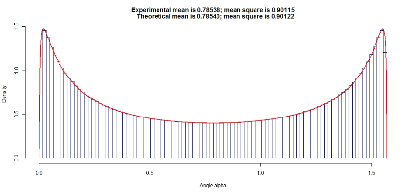
Figure 1: Density function for angle $\alpha$ in Section 1; there are zeroes at $0$ and $\pi/2$ but maximum points at $\varepsilon$ and $\pi/2-\varepsilon$, where $\varepsilon\approx 0.018363$.

2 Isosceles Triangles

The equilateral triangle $T$ with vertices

$$\begin{array}[c]{ccccc}A=\left(\dfrac{1}{3^{1/4}},-\dfrac{1}{3^{3/4}}\right),&&B=\left(-\dfrac{1}{3^{1/4}},-\dfrac{1}{3^{3/4}}\right),&&C=\left(0,\dfrac{2}{3^{3/4}}\right)\end{array}$$

is centered at $(0,0)$ and has area $1$.  Images of $T$ under $M_{r}$ for $r>0$ encompass all unit area triangles satisfying the constraint $a=b$.  It is reasonable to adopt the model $r\sim\,$Lognormal$\left(-\frac{1}{2},1\right)$ so that $\operatorname{E}(M_{r})$ is the identity matrix.  Clearly

$$a=\left|M_{r}(C-B)\right|=\sqrt{\frac{r^{2}}{\sqrt{3}}+\frac{\sqrt{3}}{r^{2}}},$$

$$b=\left|M_{r}(C-A)\right|=\sqrt{\frac{r^{2}}{\sqrt{3}}+\frac{\sqrt{3}}{r^{2}}},$$

$$c=\left|M_{r}(B-A)\right|=\sqrt{\frac{4r^{2}}{\sqrt{3}}}$$

are the sides and consequently $c\sim\,$Lognormal$\left(-\frac{1}{2}+\ln\left(\tfrac{2}{3^{1/4}}\right),1\right)$,

$$\begin{array}[c]{lll}\operatorname*{E}\left(c\right)=\dfrac{2}{3^{1/4}},&&\operatorname*{E}\left(c^{2}\right)=\dfrac{4e}{\sqrt{3}}.\end{array}$$

In Section 4, we calculate the density function for $a$ to be

$$\frac{a}{\sqrt{2\pi}}\frac{\exp\left\{-\dfrac{1}{8}\left[\ln\left(\dfrac{\sqrt{3}}{2}\left(a^{2}-\sqrt{a^{4}-4}\right)\right)+1\right]^{2}\right\}+\exp\left\{-\dfrac{1}{8}\left[\ln\left(\dfrac{\sqrt{3}}{2}\left(a^{2}+\sqrt{a^{4}-4}\right)\right)+1\right]^{2}\right\}}{\sqrt{a^{4}-4}}$$

when $a>\sqrt{2}$.  Thus the moments of $a$ are

$$\operatorname*{E}\left(a\right)=3.9753634096801809039980060...,$$

$$\operatorname*{E}\left(a^{2}\right) =\sqrt{3}\left(\frac{1}{3}+e^{2}\right)e$$

$$=36.3585711936558006990230225....$$

No closed-form expression for the mean of $a$ is known.  We have not attempted to find any densities or moments for corresponding angles.

3 Arbitrary Triangles

A disappointing aspect of the preceding two sections is the lack of any bivariate densities or cross-correlations.  We shall now remedy this situation, but a disadvantage of our third model is its artificiality.

The sides $a$, $b$, $c$ of a triangle $\Delta$ satisfy

$$16=(a+b+c)(-a+b+c)(a-b+c)(a+b-c)$$

if and only if $\Delta$ has area $1$.  The set of all solutions $(a,b,c)$ of this quartic equation is a noncompact surface $\Sigma$ in the positive octant of $\mathbb{R}^{3}$.  The orthogonal projection of $\Sigma$ into the plane $c=0$ is the region bounded (away from the origin) by the hyperbola

$$a\,b=2.$$

For example, the interior point $(a,b)=(2\cdot 3^{-1/4},2\cdot 3^{-1/4})$ of the region corresponds to the equilateral triangle ($c=2\cdot 3^{-1/4}$).  But the correspondence is not one-to-one: the point also corresponds to an isosceles triangle with apex angle $\gamma=2\pi/3$ ($c=2\cdot 3^{1/4}$).  More generally, we have

$$c=\sqrt{a^{2}+b^{2}\pm 2\sqrt{a^{2}b^{2}-4}}$$

and the two possible values of $c$ are assigned equal probability in our model. The only exceptions lie on the hyperbola itself: any boundary point of the region corresponds uniquely to a right triangle ($c=\sqrt{a^{2}+b^{2}}$).

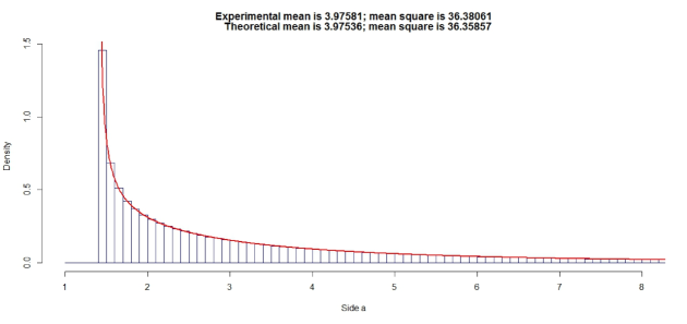
Figure 2: Density function for side $a$ in Section 2; the tail is asymptotically $O\left(\exp\left(-\frac{1}{2}\ln(a)^{2}\right)/a^{\delta}\right)$ as $a\rightarrow\infty$, where $\delta=1/2-\ln(3)/4\approx 0.225347.$

Random sampling of $a\,b\geq 2$ is performed as follows.  Generate $u$, $v$ independently according to Normal$\left(0,1\right)$.  If $u+v<0$, then reflect the point $(u,v)$ in the $xy$-plane across the diagonal line $x+y=0$; otherwise do nothing.  [The reflection is achieved via overwriting $(u,v)$ by $(-v,-u)$.]  Now translate $(u,v)$ by adding $\frac{1}{2}\ln(2)$ to each component. The density of $(u,v)$ is thus a folded bivariate normal:

$$\frac{1}{\pi}\exp\left\{-\frac{1}{2}\left[\left(u-\frac{1}{2}\ln(2)\right)^{2}+\left(v-\frac{1}{2}\ln(2)\right)^{2}\right]\right\}$$

for $u+v\geq\ln(2)$.  Let $a=e^{u}$ and $b=e^{v}$, then the bivariate density of $(a,b)$ is

$$\frac{1}{\pi}\exp\left\{-\frac{1}{2}\left[\left(\ln(a)-\frac{1}{2}\ln(2)\right)^{2}+\left(\ln(b)-\frac{1}{2}\ln(2)\right)^{2}\right]\right\}\frac{1}{a\,b}$$

for $a\,b\geq 2$.  Integrating on $b$ from $2/a$ to infinity, we obtain the univariate density of $a$:

$$\dfrac{1}{\sqrt{2\pi}}\exp\left[-\dfrac{1}{2}\left(\ln(a)-\dfrac{1}{2}\ln(2)\right)^{2}\right]\operatorname*{erfc}\left[-\frac{1}{\sqrt{2}}\left(\ln(a)-\dfrac{1}{2}\ln(2)\right)\right]\dfrac{1}{a}$$

for $a>0$, where $\operatorname*{erfc}$ is the complementary error function.  These results give rise to

$$\operatorname*{E}\left(a\right)=3.5452643891219526811143352...,$$

$$\operatorname*{E}\left(a^{2}\right)=27.2316390652988719486867211...,$$

$$\operatorname*{E}\left(a\,b\right)=10.0179601615245669326196491...$$

and, in particular, the cross-correlation coefficient between $a$ and $b$ is $\approx-0.174$.  Integrating the average of the two $c$-values

$$\dfrac{1}{2}\left(\sqrt{a^{2}+b^{2}+2\sqrt{a^{2}b^{2}-4}}+\sqrt{a^{2}+b^{2}-2\sqrt{a^{2}b^{2}-4}}\right)$$

gives $\operatorname*{E}\left(c\right)\approx 5.483$, which unfortunately demonstrates how artificial this model is.  We wish ideally for $\operatorname*{E}\left(c\right)$ to be equal to both $\operatorname*{E}\left(a\right)$ and $\operatorname*{E}\left(b\right)$, since there is no reason for one side to be preferred over the other two.  An alternative approach would involve the orthogonal projection of $\Sigma$ into the plane $c-a=0$ (rather than $c=0$), which may provide the desired symmetry.

Our goal of generating unit-area triangles analogously to unit-perimeter triangles – “throwing paint” rather than breaking a stick – remains elusive [3].  A final comment concerning Section 2 & Section 4 in [4] (based partly on [5]) is in order.  If the lengths of the three pieces (from randomly breaking the stick twice) instead are $a^{2}$, $b^{2}$, $c^{2}$ and all triangle inequalities are satisfied, then area has density function $96x$ over $[0,\sqrt{3}/12]$.  An even simpler outcome emerges if the lengths of the two pieces (from breaking the stick just once) are $a^{2}$, $b^{2}$ and angle $\gamma$ is taken to be Uniform$[0,\pi]$.  Area in this case is distributed according to Uniform$[0,1/4]$.  We wonder whether some elementary modifications of either case might lead to insight necessary to answer our question.

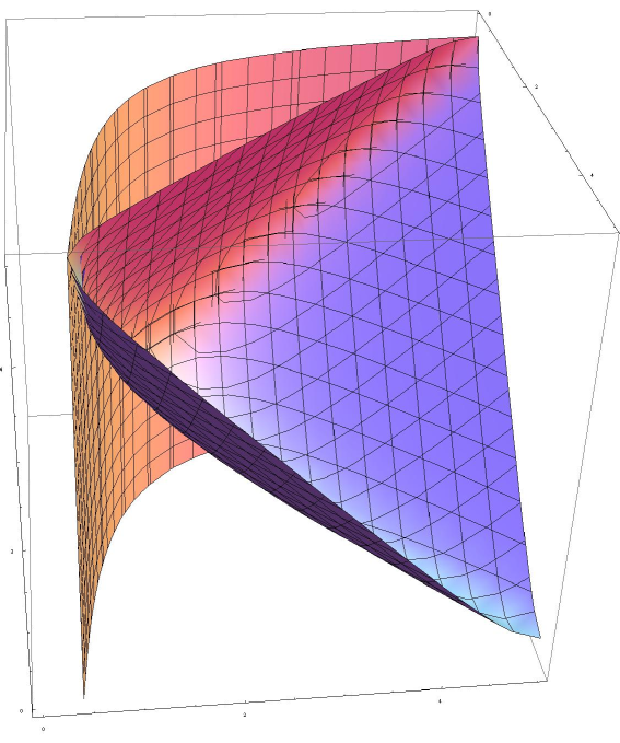
Figure 3: Surface $\Sigma$ in foreground and vertical cylinder (determined by $a\,b=2$) in background; intersection captures all right triangles.

4 Details of Calculation

We seek the distribution of the sum of a random variable $x\sim\,$Lognormal$\left(\mu,\sigma^{2}\right)$ and its reciprocal $1/x\sim\,$Lognormal$\left(-\mu,\sigma^{2}\right)$.  Solving the equation

$$x+\frac{1}{x}=y$$

for $x$ in terms of $y$, we obtain two positive values

$$\begin{array}[c]{ccc}x_{-}=\dfrac{1}{2}\left(y-\sqrt{y^{2}-4}\right)<1,&&x_{+}=\dfrac{1}{2}\left(y+\sqrt{y^{2}-4}\right)>1\end{array}$$

for $y>2$.  Because

$$\begin{array}[c]{ccccc}\dfrac{d}{dx}\left(x+\dfrac{1}{x}\right)=1-\dfrac{1}{x^{2}},&&1-\dfrac{1}{x_{-}^{2}}<0,&&1-\dfrac{1}{x_{+}^{2}}>0\end{array}$$

and

$$1-\frac{1}{x_{\mp}^{2}} =1-\dfrac{4}{\left(y\mp\sqrt{y^{2}-4}\right)^{2}}$$

$$=\dfrac{\left(y\mp\sqrt{y^{2}-4}\right)^{2}-4}{\left(y\mp\sqrt{y^{2}-4}\right)^{2}}$$

$$=\dfrac{y^{2}\mp 2y\sqrt{y^{2}-4}+\left(y^{2}-4\right)-4}{\left(y\mp\sqrt{y^{2}-4}\right)^{2}}$$

$$=\dfrac{2y^{2}\mp 2y\sqrt{y^{2}-4}-8}{\left(y\mp\sqrt{y^{2}-4}\right)^{2}}$$

$$=\dfrac{\mp 2\left(y\mp\sqrt{y^{2}-4}\right)\sqrt{y^{2}-4}}{\left(y\mp\sqrt{y^{2}-4}\right)^{2}}$$

$$=\dfrac{\mp 2\sqrt{y^{2}-4}}{y\mp\sqrt{y^{2}-4}}=\frac{\mp\sqrt{y^{2}-4}}{x_{\mp}},$$

it follows that the density function for $y$:

$$-\dfrac{1}{\sqrt{2\pi}\sigma}\frac{\exp\left\{-\dfrac{1}{2\sigma^{2}}\left[\ln\left(x_{-}\right)-\mu\right]^{2}\right\}\dfrac{1}{x_{-}}}{1-\dfrac{1}{x_{-}^{2}}}+\dfrac{1}{\sqrt{2\pi}\sigma}\frac{\exp\left\{-\dfrac{1}{2\sigma^{2}}\left[\ln\left(x_{+}\right)-\mu\right]^{2}\right\}\dfrac{1}{x_{+}}}{1-\dfrac{1}{x_{+}^{2}}}$$

simplifies to

$$\dfrac{1}{\sqrt{2\pi}\sigma}\frac{\exp\left\{-\dfrac{1}{2\sigma^{2}}\left[\ln\left(\dfrac{1}{2}\left(y-\sqrt{y^{2}-4}\right)\right)-\mu\right]^{2}\right\}+\exp\left\{-\dfrac{1}{2\sigma^{2}}\left[\ln\left(\dfrac{1}{2}\left(y+\sqrt{y^{2}-4}\right)\right)-\mu\right]^{2}\right\}}{\sqrt{y^{2}-4}}.$$

Consider now $z=\sqrt{y}$, for which $y=z^{2}$ and

$$\frac{d}{dy}\sqrt{y}=\frac{1}{2\sqrt{y}}=\frac{1}{2z};$$

the density function for $z$ is

$$\sqrt{\frac{2}{\pi}}\frac{z}{\sigma}\frac{\exp\left\{-\dfrac{1}{2\sigma^{2}}\left[\ln\left(\dfrac{1}{2}\left(z^{2}-\sqrt{z^{4}-4}\right)\right)-\mu\right]^{2}\right\}+\exp\left\{-\dfrac{1}{2\sigma^{2}}\left[\ln\left(\dfrac{1}{2}\left(z^{2}+\sqrt{z^{4}-4}\right)\right)-\mu\right]^{2}\right\}}{\sqrt{z^{4}-4}}$$

when $z>\sqrt{2}$.  As an example, if $\mu=-1/2$ and $\sigma=1$, then

$$\operatorname*{E}\left(z\right)=1.8366252372930300853898532...,$$

$$\operatorname*{E}\left(z^{2}\right) =1+e$$

$$=3.7182818284590452353602874....$$

No closed-form expression for the mean of $z=\sqrt{x+1/x}$ is known.  An attractive integral representation

$$\operatorname*{E}\left(z\right) =\dfrac{1}{\sqrt{2\pi}}{\displaystyle\int\limits_{0}^{\infty}}\sqrt{x+\frac{1}{x}}\exp\left[-\dfrac{1}{2}\left(\ln(x)+\dfrac{1}{2}\right)^{2}\right]\dfrac{1}{x}dx$$

$$=\dfrac{1}{\sqrt{\pi}}{\displaystyle\int\limits_{-\infty}^{\infty}}\sqrt{\cosh\left(u-\frac{1}{2}\right)}\exp\left(-\frac{1}{2}u^{2}\right)du$$

(found via $u-1/2=\ln(x)$) does not seem to help.

The arguments provided here can be extended to find the density function of $w=\sqrt{x^{2}/\kappa+\kappa/x^{2}}$ for any $\kappa>0$:

$$\frac{w}{\sqrt{2\pi}\sigma}\frac{\exp\left\{-\dfrac{1}{8\sigma^{2}}\left[\ln\left(\dfrac{\kappa}{2}\left(w^{2}-\sqrt{w^{4}-4}\right)\right)-2\mu\right]^{2}\right\}+\exp\left\{-\dfrac{1}{8\sigma^{2}}\left[\ln\left(\dfrac{\kappa}{2}\left(w^{2}+\sqrt{w^{4}-4}\right)\right)-2\mu\right]^{2}\right\}}{\sqrt{w^{4}-4}}$$

when $w>\sqrt{2}$.  The case $\kappa=\sqrt{3}$, $\mu=-1/2$ and $\sigma=1$ gives the density function for $a$ in Section 2.  As another example, if $\kappa=1$ instead, then

$$\operatorname*{E}\left(w\right)=3.3278221244164268180344110...,$$

$$\operatorname*{E}\left(w^{2}\right) =\left(1+e^{2}\right)e$$

$$=22.8038187516467129762888171....$$

Again, an attractive integral representation

$$\operatorname*{E}\left(w\right)=\dfrac{1}{\sqrt{\pi}}{\displaystyle\int\limits_{-\infty}^{\infty}}\sqrt{\cosh\left(2v-1\right)}\exp\left(-\frac{1}{2}v^{2}\right)dv$$

does not seem to help.  For reasons of brevity, we omit proof of the general formula.

Much more relevant material can be found at [6], including experimental computer runs that aided theoretical discussion here.

5 Addendum

Continuing a thought raised at the end of Section 3, define a new coordinate system $\tilde{a}$, $\tilde{b}$, $\tilde{c}$ via a $45^{\circ}$-rotation:

$$\begin{array}[c]{ccccc}a=\dfrac{1}{\sqrt{2}}\left(\tilde{a}-\tilde{c}\right),&&b=\tilde{b},&&c=\dfrac{1}{\sqrt{2}}\left(\tilde{a}+\tilde{c}\right)\end{array}$$

then the orthogonal projection of $\Sigma$ into the plane $\tilde{c}=0$ is the region bounded (away from the origin) by

$$\left(2\tilde{a}^{2}-\tilde{b}^{2}\right)\tilde{b}^{2}=16.$$

We note that the boundary is well-approximated, for large $\tilde{a}$, by $\tilde{b}=\sqrt{2}\tilde{a}$ from above and $\tilde{b}=2\sqrt{2}/\tilde{a}$ from below.  Ideas for natural random sampling of $\left(2\tilde{a}^{2}-\tilde{b}^{2}\right)\tilde{b}^{2}\geq 16$, akin to $a\,b\geq 2$ earlier, would be welcome.

References

- [1] M. Baker, A collection of formulae for the area of a plane triangle, Annals of Math. v. 1 (1885) n. 6, 134–138; v. 2 (1885) n. 1, 11–18.
-
[2]
K. Conrad, Decomposing ,
http://www.math.uconn.edu/~kconrad/blurbs/grouptheory/SL(2,R).pdf. - [3] S. R. Finch, Random triangles. VI, unpublished note (2011), http://www.people.fas.harvard.edu/~sfinch/.
- [4] S. R. Finch, Uniform triangles with equality constraints, http://arxiv.org/abs/1411.5216.
- [5] A. Edelman and G. Strang, Random triangle theory with geometry and applications, Found. Comput. Math. (to appear); http://www-math.mit.edu/~edelman/homepage/papers/focm.pdf.
-
[6]
S. R. Finch, Simulations in R involving triangles and
tetrahedra, http://www.people.fas.harvard.edu/~sfinch/csolve/rsimul.html.
Steven Finch Dept. of Statistics Harvard University Cambridge, MA, USA steven_finch@harvard.edu