Magnetically-driven crustquakes in neutron stars

Abstract

Crustquake events may be connected with both rapid spin-up ‘glitches’ within the regular slowdown of neutron stars, and high-energy magnetar flares. We argue that magnetic field decay builds up stresses in a neutron star’s crust, as the elastic shear force resists the Lorentz force’s desire to rearrange the global magnetic-field equilibrium. We derive a criterion for crust-breaking induced by a changing magnetic-field configuration, and use this to investigate strain patterns in a neutron star’s crust for a variety of different magnetic-field models. Universally, we find that the crust is most liable to break if the magnetic field has a strong toroidal component, in which case the epicentre of the crustquake is around the equator. We calculate the energy released in a crustquake as a function of the fracture depth, finding that it is independent of field strength. Crust-breaking is, however, associated with a characteristic local field strength of $2.4\times 10^{14}$ G for a breaking strain of $0.001$, or $2.4\times 10^{15}$ G at a breaking strain of $0.1$. We find that even the most luminous magnetar giant flare could have been powered by crustal energy release alone.

1 Introduction

The crust of a neutron star (NS) is a rigid elastic shell around a kilometre thick, which connects the supranuclear-density fluid core with the star’s magnetosphere, and in turn any observable phenomena. As for any elastic medium, however, there is a maximum strain it can sustain – beyond which the crust will yield locally, causing seismic activity or ‘crustquakes’.

A crustquake scenario related to changes in rotational strain was suggested shortly after the discovery of radio pulsars, as a way to explain observations that the otherwise stable spindown of a pulsar can be interrupted by abrupt increases – ‘glitches’ – in spin frequency and spin-down rate (Baym et al., 1969). The idea is that the rotational oblateness at the star’s birth is frozen into the crust; as the star spins down it wants to become more spherical, and the overly-oblate crust develops strains which eventually break it and cause an increase in angular momentum of the crust. This mechanism alone, however, cannot explain the observed timing behaviour; instead, in the currently standard glitch scenario the spin-up is attributed to a sudden transfer of angular momentum from a more rapidly rotating superfluid component to the rest of the star (Anderson & Itoh, 1975). Nonetheless, crustquakes are often invoked in glitch models, either as a trigger for these sudden angular-momentum transfer events (Link & Epstein, 1996; Eichler & Shaisultanov, 2010) or to explain the persistent changes in spin-down rate seen after some glitches (Alpar et al., 1994).

\psfrag{decay}{{\bf field decay/rearrangement}}\includegraphics[width=433.62pt]{figs/crust-crack-new.eps}

Figure 1: Cartoon of crust-breaking scenario. For clarity we have shown the motion of an equatorial region of magnetic flux to represent field rearrangement, but the argument is applicable to any local changes in the field anywhere in the crust. We assume the young NS has reached a hydromagnetic equilibrium by the time the crust freezes, so that the crust does not initially need to support any stresses (left-hand plot). At some later point in the star’s evolution the magnetic field has lost energy and would need to adjust to remain in a global fluid equilibrium, but whilst this adjustment may take place in the fluid core, it is resisted by shear stresses in the crust (middle plot). The magnetically-induced stresses to the crust build, and eventually some region of the crust will exceed its yield strain and break (right-hand plot). The local magnetic field will be able to return to a fluid equilibrium again.

In addition to these rotational effects, magnetic stresses will also develop in the crust throughout a NS’s lifetime, as a result of internal magnetic field evolution. For typical radio pulsars such stresses might be negligible, since the crust’s elastic energy exceeds the magnetic energy, and the elastic force dominates the Lorentz force. For highly magnetised NSs however, like magnetars – objects with inferred dipole magnetic fields at least as high as $\sim\!10^{15}$ G – the two energies are comparable, and it is quite feasible that magnetic stresses could be strong enough to induce crust-yielding: crustquakes or plastic flow. Such magnetically-driven seismic activity forms the core of the widely-accepted model for magnetar activity, firstly put forward by Thompson & Duncan (1995) to explain bursts in anomalous X-ray pulsars (AXPs) and the bursts and gamma-ray giant flares in soft-gamma ray repeaters (SGRs). The recurrent bursts in magnetars have characteristic durations in the range $\sim\!0.01-1\ \rm{s}$ and peak luminosities up to $10^{41}\ \rm{erg\ s}^{-1}$, and are in many cases associated with glitches or other timing anomalies (Woods & Thompson, 2006; Dib & Kaspi, 2014). The potential connection with crustquakes is consistent with the observation that the burst-energy distribution in magnetars follows a power law (Cheng et al., 1996; Göǧüş et al., 2000), similar to that of earthquakes.

Recent observations are indicative of a continuum of activity in radio pulsars and magnetars (Kaspi, 2010): SGRs have been discovered with weak inferred dipole fields (see, e.g. Rea et al. (2010)), and magnetar-like activity has been seen from some (otherwise rotationally-powered) radio pulsars, such as the burst and coincident glitch in J1846-0258 (Gavriil et al., 2008; Kuiper & Hermsen, 2009). This has led to considerable efforts to explain the different phenomenologies of NSs in a unified scheme by studying the thermal and magnetic-field evolution in their crusts (Perna & Pons, 2011; Pons & Rea, 2012). These first results suggest that seismic activity induced by magnetic field evolution is of relevance not only for magnetars, but also rotationally-powered pulsars.

Motivated by the many possible observational manifestations of crustal stresses in a NS, we study a mechanism in which a rearranging global magnetic field provides the source of these stresses, eventually causing the crust to yield. We derive a condition for magnetically-induced crustal failure based on the von Mises criterion for the yielding of elastic media. Using a variety of different magnetic-field models, including NSs with normal and superconducting cores and with a force-free magnetosphere, we study the crustal strain patterns that these field configurations would produce and the point at which regions of the crust will yield. We find a relationship between the depth of a crustal fracture, the breaking strain and the corresponding energy release, and deduce a characteristic field strength associated with crustquakes. We argue that magnetically-induced crustquakes could power even the most luminous magnetar phenomena, contrary to previous suggestions, as well as operate in NSs with less exceptional inferred dipole magnetic field strengths.

2 Magnetic-field equilibrium sequences

Around a day into its life a neutron star begins to form a crust, crystallising gradually from the inside out over the course of the following century. Before the crust has even begun to form, however, it is reasonable to expect the magnetic field to have reached an equilibrium with the fluid star, since the timescale of this process will be the same order of magnitude as an Alfvén-wave crossing time (around a second for typical NS parameters and a $10^{14}$ G field; shorter for stronger fields). The crust will thus freeze in a relaxed state threaded by its early-stage magnetic field; in the absence of shear stresses the equilibrium description of this phase will just be that of a magnetised fluid body (left panel of figure 1). Over time the star will gradually lose magnetic energy through secular decay processes; see section 3. The magnetic field will want to adjust to a new fluid equilibrium, but its rearrangement will be inhibited by the crust’s rigidity (middle plot of figure 1). The magnetically-induced stresses in the crust will thus grow over time, and eventually exceed the elastic yield value; when this happens the crust will break in the region where its breaking strain has been exceeded, and the field will be able to return (locally) to its fluid equilibrium configuration, depicted in the right-hand panel of figure 1. The stress that builds up in a NS’s crust will thus be sourced by the difference between the field configuration present when the crust froze, and the magnetic field’s desired present equilibrium, which it is prevented from reaching by shear stresses. Both the ‘before’ and the (desired) ‘after’ magnetic-field configurations are therefore fluid equilibria, so by comparing two such equilibria with different values of magnetic energy we can determine the expected stresses built up in an elastic crust. A quantitative description of the above scenario is given in section 4.2, and its potential shortcomings are discussed in the following subsection, 4.3.

To explore the possible range of these ‘before’ and ‘after’ magnetic-field configurations during the evolution of a highly-magnetised neutron star, we consider three classes of neutron-star model: accounting for the possibilities that the core protons are superconducting or not, and considering a scenario where the star has a magnetar-like magnetosphere in equilibrium with its interior field (and matches smoothly to it at the stellar surface). From these various plausible models of a NS’s field configuration we hope to look for universal features and also possible differences in how the crust breaks which could be used to distinguish between them.

Our model NS is composed of protons, neutrons and electrons, but the electrons have negligible inertia and their chemical potential can simply be added as an extra contribution to that of the protons. We are then left with a two-fluid core of protons and superfluid neutrons, matched at $0.9$ times the stellar radius $R_{*}$ to a non-superconducting and unstrained crust. We capture these features by confining the neutron fluid to the region between the centre and $0.9R_{*}$, while having the proton fluid extend from the centre out to the stellar surface, so that the shell from $0.9R_{*}$ to $R_{*}$ is a single-fluid region. Since a relaxed elastic medium obeys the same equilibrium equations as a fluid, we can thus regard the proton fluid in this outer single-fluid region as a ‘crust’ (Prix, Novak & Comer, 2005). The equation of state we choose is effectively a double polytrope (Lander, Andersson & Glampedakis, 2012), setting the proton and neutron polytropic indices $N_{\textrm{p}},N_{\textrm{n}}$ to values of $1.5$ and $1.0$ respectively, to mimic a ‘realistic’ core proton-fraction profile in the core (e.g. that of Douchin & Haensel (2001)). Since the polytropic indices of the two fluids are different, the stellar models have composition-gradient stratification. The neutron-density profile has, however, negligible impact on these configurations. Finally, although it would naturally be more desirable to work directly with a tabulated equation of state, instead of our double-polytrope approximation to one, we do not believe that doing so would have any serious impact on our results; see the discussion in section 4.1.

The code we use to calculate equilibria works in dimensionless units, and physical values given here come from redimensionalising code results to one particular model star of $1.4$ solar masses and with fixed neutron and proton polytropic constants of $k_{\textrm{n}}=5.65\times 10^{4}\ \textrm{g}^{-1}\textrm{cm}^{5}\textrm{s}^{-2}$ and $k_{\textrm{p}}=2.74\times 10^{10}\ \textrm{g}^{-2/3}\textrm{cm}^{4}\textrm{s}^{-2}$ respectively. For our chosen neutron and proton density profiles these values produce a star with radius of 12 km (varying very slightly with field strength). Note that since all our models have the same mass and the same equation of state (i.e. fixed polytropic indices and constants), they correspond to the same physical star – allowing for a direct comparison between different models.

In all cases we are interested in mixed poloidal-toroidal magnetic-field configurations, since these are the most generic models and also the most likely to be stable (Tayler, 1980). Although the toroidal-field component can be locally strong in our models, its contribution to the total magnetic energy is always small compared with the poloidal one. The equilibrium models we consider here are all chosen to have the strongest possible toroidal component; as we will see later in section 4, this allows us to put an upper limit on how readily the crust will yield.

The key differences between our three classes of model come from the form of the magnetic force $\boldsymbol{\mathfrak{F}}_{\textrm{mag}}$, and the electric current distribution; we discuss each case next and show example field configurations, all with a polar-cap field strength $B_{p}=6.0\times 10^{14}$ G for direct comparison.

2.1 Normal core protons, vacuum exterior

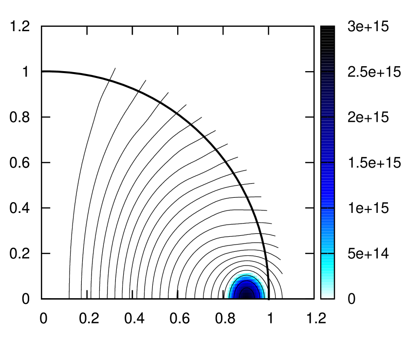
Figure 2: Magnetic-field configuration for a model magnetar with a polar-cap field strength $B_{p}=6.0\times 10^{14}$ G and a total magnetic energy of $6.8\times 10^{47}$ erg. The core is a two-fluid system of superfluid neutrons and normal protons, matched to a normal crust at a dimensionless radius $r/R_{*}=0.9$. The thick black arc at $r/R_{*}=1$ represents the stellar surface. We plot the poloidal-field lines, denoting the direction of this field component, whilst the colour scale shows the magnitude of the toroidal component, whose direction is azimuthal – into/out of the page.

This is the simplest case, where both the core protons and the crust are subject to the familiar Lorentz force for normal (non-superconducting) matter:

$$\boldsymbol{\mathfrak{F}}_{\textrm{mag}}=\frac{1}{4\pi}(\nabla\times{\bf{B}})\times{\bf{B}},$$ (1)

where ${\bf{B}}$ is the magnetic field. Note that the neutron fluid does not feel any magnetic force. We assume that the exterior of the star is a vacuum, with no charged particles able to carry an electric current, so that Ampère’s law simply imposes a restriction on the form of the external magnetic field ${\bf{B}}_{\textrm{ext}}$:

$$\nabla\times{\bf{B}}_{\textrm{ext}}=0.$$ (2)

An alternative way to look at this condition is that there could be magnetospheric currents, but that they do not communicate with the interior and therefore do not affect its equilibrium. One could justify this rather simplistic model by suggesting that the magnetic field in a magnetar’s core is strong enough to break proton superconductivity (Baym, Pethick & Pines, 1969a; Sinha & Sedrakian, 2014), so that the normal-matter equations would apply. One key motivation for us, however, is that it allows us to produce configurations with stronger toroidal components than in our other cases; see figure 2. We believe the reason for this to be numerical rather than physical – our code’s iterative scheme converges to strong-toroidal-field solutions more readily in this case than for the other two models considered in this paper. This class of model is constructed using the techniques described in Lander, Andersson & Glampedakis (2012), although the resultant field configurations are not dissimilar to those of single-fluid models.

2.2 Superconducting core protons, vacuum exterior

Our next class of equilibrium models are constructed as described in Lander (2014). These consist of a core of superfluid neutrons and type-II superconducting protons, matched to a normal crust. In the crust, the magnetic field is smoothly distributed (on a microscopic scale) and the magnetic force is just the Lorentz force (1), acting on the entire crust. In the core, by contrast, the effect of proton superconductivity is to quantise the field into an array of thin fluxtubes; on the macroscopic level, this produces a different magnetic force. Unlike the Lorentz force, which depends only on the macroscopic field ${\bf{B}}$, the magnetic force for a type-II superconductor also involves the lower critical field ${\bf H}_{c1}$, related to the magnetic field along fluxtubes (Easson & Pethick, 1977; Akgün & Wasserman, 2008; Glampedakis, Andersson & Samuelsson, 2011). This latter field is parallel to ${\bf{B}}$ and proportional to the local proton density: in the centre, where the proton density is highest, it reaches $10^{16}$ G, but is on average around $10^{15}$ G within the core, irrespective of the value of ${\bf{B}}$. The most important feature governing these equilibria is the difference in the form of the magnetic force for the core and crust:

$$\boldsymbol{\mathfrak{F}}_{\textrm{mag}}=\left\{\begin{split}&\frac{1}{4\pi}(\nabla\times{\bf H}_{c1})\times{\bf{B}}-\frac{\rho_{\mathrm{p}}}{4\pi}\nabla\left({B\frac{\partial{H_{c1}}}{\partial{\rho_{\mathrm{p}}}}}\right)&\ \ \textrm{(core)}\\ &\frac{1}{4\pi}(\nabla\times{\bf{B}})\times{\bf{B}}&\ \ \textrm{(crust)}\\ \end{split}\right.$$ (3)

Our models assume the core and crustal fields match without any current sheet in this region, and as for the models described in the previous subsection do not have any exterior current. An example of a model with core proton superconductivity is shown in figure 3.

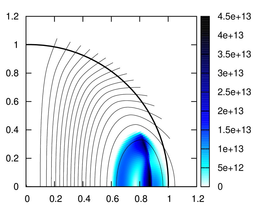
Figure 3: Magnetic-field configuration for a model NS with $B_{p}=6.0\times 10^{14}$ G, with a superfluid-superconducting core matched to a normal crust. The total magnetic energy for this model is $3.1\times 10^{48}$ erg. The crust-core boundary and surface are at dimensionless radii of $0.9$ and $1.0$ as before; and again, we plot poloidal field lines in black and toroidal-field magnitude with the colour scale. Note the weakness of the toroidal component compared with the normal-matter model in figure 2.

2.3 Normal core protons, magnetosphere

These equilibria are constructed in the same way as the models with a normal core, except that we now allow for a toroidal-field component that extends outside the star. This is sourced by a poloidal electric current in a magnetosphere of charged particles, located in a lobe around the equator as argued for by Beloborodov & Thompson (2007). Outside the lobe region there is vacuum, where the field obeys $\nabla\times{\bf{B}}_{\textrm{ext}}=0$, but within it there is a force-free region with

$$\nabla\times{\bf{B}}_{\textrm{ext}}=\alpha{\bf{B}}_{\textrm{ext}},$$ (4)

where $\alpha$ is a function constant along magnetic-field lines, governing the distribution of magnetospheric current; see Glampedakis, Lander & Andersson (2014) for details on the method of solution for these configurations. In figure 4 we plot two such models of NSs in dynamical equilibrium with their magnetosphere, both with $B_{p}=6.0\times 10^{14}$ G, but with $2.5\times 10^{46}$ erg of magnetic energy removed from the toroidal component in the second plot, illustrating how the magnetosphere rearranges in this case.

\psfrag{before}{initial state}\psfrag{after}{after magnetospheric decay}\includegraphics[width=433.62pt]{figs/magneto_6e14.eps}

Figure 4: Two magnetic-field configurations for a normal-matter NS with a current-carrying corona and $B_{p}=6.0\times 10^{14}$ G, but with the lower plot having $2.5\times 10^{46}$ erg less magnetic energy. All of this energy has been taken out of the toroidal component, visibly altering the magnetosphere. The toroidal component attains a maximum value greater than that of the model in figure 3, but still less than that in figure 2. The lower model has $5.4\times 10^{47}$ erg of magnetic energy.

At this point it is worth speculating about scenarios for the formation of an equatorial corona of current-carrying plasma, although this is not the focus of our work. The standard argument for the formation of such a corona (Beloborodov & Thompson, 2007) assumes the interior field evolves in such a way that it wishes to ‘eject magnetic helicity’ – equivalently, to induce an electric current in the environs of the star. For a mature NS this process cannot happen immediately, but initially results in crustal stresses building – when these are released the initially poloidal field is twisted in an azimuthal direction, thus generating a toroidal component.

As shown in Glampedakis, Lander & Andersson (2014), given a sufficiently dense corona of charged particles, the star can form a magnetosphere which is in dynamical equilibrium with the internal field and hence supported by a relaxed crust, as opposed to one which has to shear to generate the field. If we assume the toroidal component is always confined to the same flux surface (poloidal field line), then the decay of this field would cause the magnetosphere to change shape, moving in towards the crust. As before, the magnetic flux’s inward motion would initially be inhibited by shear forces, but at a later stage the induced stresses could grow large enough to break the crust. Figure 4 assumes a scenario like this, where the configuration of the upper panel decays into that of the lower panel.

One could also view the panels in reverse, however, where an internal toroidal field wishes to rise out of the star for whatever reason, but is again inhibited by the crust. Clearly one cannot view the specific configurations of figure 4 as representing this scenario, since that would require an increase in magnetic energy, but qualitatively similar solutions with decreasing magnetic energy could be constructed. In terms of a changing global equilibrium this way round seems less likely, but it does broadly represent the corona-formation mechanism discussed in Beloborodov & Thompson (2007) and Beloborodov (2009). Note that the strain patterns that would build by running the scenario in this order would be the same as in the reverse order, however, since the strain/yield criterion of section 4.2 remains the same if the ‘before’ and ‘after’ configurations are swapped around.

3 Field decay

The fact that NS magnetic fields do decay is well-established, from both theoretical and observational study; our knowledge of the relative importance of different decay mechanisms, and their corresponding timescales, is nevertheless surprisingly incomplete. If the activity of young NSs like magnetars is powered by field decay, however, there must be at least one rather rapidly-acting decay mechanism. We therefore consider it reasonable to assume magnetically-induced stresses will build in a NS crust on a timescale short enough to be astrophysically relevant, even if current theoretical uncertainties prevent us from pinpointing the mechanism(s) which will most readily build these stresses. Here we briefly review the literature on magnetic-field evolution to highlight the most promising mechanisms for relatively rapid changes in a NS’s field.

The most familiar source of magnetic field dissipation is Ohmic decay, which in terrestrial materials and the neutron-star crust is the macroscopic result of electrons scattering off a solid material’s ion lattice, thus heating it and reducing the electric current. Ohmic decay operates more rapidly on small-scale fields than large-scale ones. In the crust of a NS the separate process of Hall drift acts to redistribute the magnetic flux into structures of progressively shorter lengthscales (Goldreich & Reisenegger, 1992); although this process is not itself dissipative it aids Ohmic decay, which acts more rapidly on small-scale magnetic fields.

For the core, many studies have argued that the evolution is likely to be very slow. Ohmic decay itself must be restricted to the thin cores of normal protons at the centre of fluxtubes – these cores comprise a minute volume of the NS core, which is otherwise in a superconducting state, and so this decay mechanism is expected to be extremely slow (Baym, Pethick & Pines, 1969b). Ambipolar diffusion – a drift of the charged particles, and hence the magnetic field, with respect to the neutrons – is both dissipative and acts to move the core magnetic field outwards into the crust (Goldreich & Reisenegger, 1992). However, accounting for the superfluid state of the neutrons drastically increases its timescale (Glampedakis, Jones & Samuelsson, 2011).

For magnetic fields $B<H_{c1}\approx 10^{15}$ G, the Meissner effect is expected to expel core magnetic flux to the crust-core boundary, a region of (probably) higher electrical resistivity and hence faster Ohmic decay. More precisely, the Meissner effect dictates that the eventual equilibrium state of the field will be one where it is exponentially screened from the core over some short lengthscale – it does not specify the dynamical mechanism which might achieve this, nor the timescale. Different mechanisms have been invoked for the transport of magnetic flux out of the core. The fluxtubes may move out of the core through mutual self-repulsion (Kocharovsky, Kocharovsky & Kukushkin, 1996), driven by a buoyancy force (Muslimov & Tsygan, 1985; Wendell, 1988; Harrison, 1991; Jones, 1991), or dragged by the outwardly-moving neutron vortices as the star’s rotation rate decreases (Ding, Cheng & Chau, 1993). The result of these various studies is an assortment of prospective timescales for field decay which range over at least eight (!) orders of magnitude ($10^{4}-10^{12}$ yr). Nonetheless the consensus, inasmuch as there is one, points to a rather slow core evolution and suggests that observed field decay is crustal in origin.

Slow core-field evolution may, however, be contradicted by the observation that young NSs like magnetars are able to build and release huge stresses: the most energetic giant flare ($\sim\!10^{46}\ \textrm{erg}$) came from a magnetar believed to be under a thousand years old (Palmer et al., 2005; Tendulkar, Cameron & Kulkarni, 2012). Alternatively, instead of being the result of secular stress build-up, magnetar giant flares may be the manifestation of a rapidly-acting hydromagnetic instability (Thompson & Duncan, 1996; Ioka, 2001) – although that in itself requires the instability to be somehow suppressed until some critical point, and therefore one might again have to invoke the build-up of crustal stresses. There is clearly more work to be done in attempting to achieve some kind of consensus on the role of magnetic field decay in NS phenomena – but if crustquakes induce magnetar activity, as discussed in this paper, we may in fact be able to use observations to determine a core field decay timescale and hence reduce the discordance of the theoretical models.

4 Magnetically-induced crustquakes

4.1 Crustal properties

To obtain quantitative results about how a magnetic field can act to strain and eventually break a neutron-star crust, we need a realistic model of this region – in particular, for the crustal shear modulus and breaking strain. In our equilibrium models, described in section 2, we used a double-polytrope equation of state designed to mimic a ‘realistic’ core proton fraction, but unfortunately this results in an unrealistically low density crust. The crustal density distribution does not have a strong impact on the magnetic field configuration, but is important for calculating a reasonable shear-modulus profile. Accordingly, we choose to take quantities from a tabulated, ‘realistic’, equation of state (Douchin & Haensel, 2001), and by doing so we can take advantage of a recent shear-modulus fitting formula based on the results of molecular-dynamics simulations (Horowitz & Hughto, 2008).

Using a polytropic crust model to calculate magnetic-field equilibria, but then adopting parameters from a tabulated equation of state to calculate the shear modulus, is clearly not consistent. Nonetheless, we argue next that the level of inconsistency is justifiable to our order of working. We use our equilibrium calculations solely to get models of the magnetic field and not, for example, pressure or density profiles. Had we employed the Douchin-Haensel equation of state consistently throughout this work – i.e. for our equilibrium calculations too – we would have obtained somewhat different magnetic-field distributions. The degree of inconsistency in our approach in this paper, therefore, depends on the difference between equilibria calculated using our polytropic models and those calculated with the equation of state of Douchin & Haensel (2001) – and this difference should be small, since the dependence of magnetic-field distributions on the stellar equation of state is in fact quite weak (Yoshida, Yoshida & Eriguchi, 2006).

\psfrag{log_mu}{$\displaystyle\log\left({\frac{\mu}{\textrm{dyn\ cm}^{-2}}}\right)$}\psfrag{r_dimless}{$r/R_{*}$}\includegraphics[width=433.62pt]{figs/shear_mod.eps}

Figure 5: The profile of the shear modulus $\mu$ throughout the crust, calculated using equation (6) – a fitting formula based on the results of molecular-dynamics simulations (Horowitz & Hughto, 2008). The required crustal input quantities (for example, the variation of atomic number within the crust) come from polynomial fits to the tabulated equation of state of Douchin & Haensel (2001), and our magnetar temperature profile is taken from Kaminker et al. (2009).

4.1.1 Shear modulus

From the Douchin-Haensel tabulated equation of state we make simple polynomial fits to the radial dependence of the baryon number $n_{b}$, atomic weight $A$, atomic number $Z$ and free neutron fraction $x_{\textrm{n}}^{\textrm{free}}$ in the crust. We fit our temperature profile to results for a 1000-year-old magnetar from Kaminker et al. (2009) (see their figure 6; we use their profile for the lower of the two heat intensities, with a heat source at the top of the inner crust). The maximum temperature slightly exceeds $10^{9}$ K. Our fitting formulae approximate crustal parameters over the density range $0.05\rho_{\textrm{cc}}<\rho<\rho_{\textrm{cc}}$ (where $\rho_{\textrm{cc}}$ is the density at the crust-core boundary) and may deviate from the correct behaviour below this density. On our numerical grid the crust is covered by $24$ radial points, meaning that our fitting formulae are designed to approximate all but the outermost four points – precise enough for our purposes.

To calculate crustal properties, we first note that the ion number density in the crust $n_{i}=n_{b}(1-x_{\textrm{n}}^{\textrm{free}})/A$, from which we define the ion sphere radius $a_{i}=(4\pi n_{i}/3)^{-1/3}$. The Coulomb coupling parameter $\Gamma$ is then given by

$$\Gamma=\frac{(Ze)^{2}}{a_{i}T},$$ (5)

where $e$ is the elementary charge (i.e. of a proton). From the various crustal properties discussed above, we are now in a position to determine the shear modulus $\mu$ of our model NS crust using the formula from Horowitz & Hughto (2008):

$$\mu=\left({0.1106-\frac{28.7}{\Gamma^{1.3}}}\right)\frac{n_{i}}{a_{i}}(Ze)^{2}.$$ (6)

The resulting shear modulus profile we use is shown in figure 5. At the innermost crustal gridpoint $\mu=2.4\times 10^{30}$ dyn cm^-2 – a little higher than the crust-core value of $\mu=1.8\times 10^{30}$ dyn cm^-2 from Hoffman & Heyl (2012) and the classic estimate of $\mu\approx 10^{30}$ dyn cm^-2 (Ruderman, 1969).

4.1.2 Breaking strain

Recent molecular-dynamics simulations indicate that the neutron-star crust is considerably stronger than previously thought (Horowitz & Kadau, 2009; Hoffman & Heyl, 2012), with a breaking strain $\sigma_{\textrm{max}}$ around $0.1$ (dimensionless, since a strain is a fractional deformation; a ratio of two lengths). $\sigma_{\textrm{max}}$ is essentially temperature-independent as long as one is well above the melting temperature (whose value corresponds to $\Gamma\approx 175$); it is also independent of density, except perhaps in a narrow region of ‘nuclear pasta’ at the crust-core boundary (Ravenhall, Pethick & Wilson, 1983); and neither impurities nor strain rate have a significant impact on it. Accordingly, taking the breaking strain as constant is a good first approximation (Horowitz, 2015). Note that the breaking stress, by contrast, is a dimensional quantity (with units of pressure) and has significant variation within the crust (Chugunov & Horowitz, 2010). In this paper we adopt two canonical values for the breaking strain: $\sigma_{\textrm{max}}=0.1$ to reflect recent simulations, and $\sigma_{\textrm{max}}=0.001$ to compare with earlier work.

4.2 A criterion for magnetically-induced crustquakes

We are interested in how magnetic field decay/rearrangement causes strain to build in a neutron star’s crust, and where and when this strain might finally cause the crust to break. Since there is no reason to expect the magnetic field to be uniform – or to decay/rearrange uniformly – the built-up strains will vary greatly within the crust. Previous crust-breaking criteria based on global estimates (Thompson & Duncan, 1995; Hoffman & Heyl, 2012) are therefore not only somewhat crude, but also give no idea of where the crust will fail. We aim to improve on these by using a criterion, which we derive next, accounting for the local changes in magnitude and direction of the field.

To simplify the algebra in the derivation which follows, we use standard tensor index notation, denoting tensor indices with $i$ and $j$. We start with the general stress tensor for the crust in our model:

$$\tau_{ij}=-pg_{ij}+\mu\sigma_{ij}+\mathcal{M}_{ij},$$ (7)

where $p$ is fluid pressure, $g_{ij}$ the flat-space 3-metric, $\sigma_{ij}$ the elastic strain tensor and $\mathcal{M}_{ij}$ the Maxwell (magnetic) stress tensor. In this problem we are only considering equilibrium configurations — either strained or unstrained — so the sum of the stresses should balance: $\tau_{ij}=0_{ij}$, where $0_{ij}=0\ \forall\{i,j\}$.

We assume the NS’s crust freezes in a relaxed state, with a certain magnetic energy and polar-cap field strength; quantities pertaining to this state will be denoted with a subscript or superscript zero in the following derivation. With no shear forces present, the equilibrium at this stage is that of a fluid body:

$$0_{ij}=-p^{0}g_{ij}+\mathcal{M}^{0}_{ij}.$$ (8)

Over the star’s lifetime, different secular processes (see previous section) act to reduce the magnetic energy, so that the star’s evolution can be described by a sequence of quasi-static equilibria, with incrementally smaller values of magnetic energy. These are no longer fluid equilibria, however, as the crust resists any adjustment of the magnetic field by balancing the Lorentz forces by its elastic shear force:

$$0_{ij}=-pg_{ij}+\mu\sigma_{ij}+\mathcal{M}_{ij}.$$ (9)

The magnetically-induced change to the fluid pressure $p$ will be tiny, and so the difference between its initial value and that at a later time may safely be neglected, i.e. $p^{0}-p\approx 0$. The strain in the crust is thus entirely sourced by the difference in the Maxwell stress tensor between initial and later field configurations:

$$\mu\sigma_{ij}=\mathcal{M}^{0}_{ij}-\mathcal{M}_{ij}.$$ (10)

The magnetically-induced stresses in the crust gradually grow, and are largest where the field wishes to adjust the most. For sufficiently strong magnetic fields and sufficient readjustment, the crust will yield in some region, allowing the magnetic field in the affected region to return to a fluid equilibrium; recall the cartoon in figure 1.

To proceed we need the explicit form of $\mathcal{M}_{ij}$. Since the crust is not superconducting this is the familiar Maxwell stress tensor:

$$\mathcal{M}_{ij}=\frac{1}{4\pi}\left({B_{i}B_{j}-\frac{1}{2}B^{2}\delta_{ij}}\right).$$ (11)

Note that taking the divergence of this tensor gives:

$$\nabla\cdot\mathcal{M}=\frac{({\bf{B}}\cdot\nabla){\bf{B}}}{4\pi}-\frac{\nabla B^{2}}{8\pi},$$ (12)

the Lorentz force, as expected.

The von Mises criterion predicts that an isotropic elastic medium will yield when

$$\sqrt{\textstyle{\frac{1}{2}}\sigma_{ij}\sigma^{ij}}\geq\sigma_{\textrm{max}}.$$ (13)

This is not, strictly speaking, a criterion for breaking; ‘yield’ means only that the crust ceases to respond elastically to additional strains, but may enter a regime of plastic flow before actually breaking. We ignore the distinction between these two responses for now, and use the terms ‘yield’ and ‘break’ interchangeably. For the purposes of our work the distinction is not so important, as we anticipate both breaking and plastic flow to release the same total amount of pent-up magnetic energy, but perhaps in characteristically different ways and over different timescales; see section 5.

Now, from equations (10) and (11):

$$\sigma_{ij}\sigma^{ij} =\frac{1}{\mu^{2}}\left({\mathcal{M}^{0}_{ij}\mathcal{M}^{ij}_{0}+\mathcal{M}_{ij}\mathcal{M}^{ij}-\mathcal{M}^{0}_{ij}\mathcal{M}^{ij}-\mathcal{M}_{ij}\mathcal{M}^{ij}_{0}}\right)$$

$$=\frac{1}{64\pi^{2}\mu^{2}}\left({2B^{2}B_{0}^{2}+3B^{4}+3B_{0}^{4}-8({\bf{B}}\cdot{\bf{B}}_{0})^{2}}\right).$$ (14)

The von Mises criterion (13) applied to the case of crust-yielding sourced by a changing magnetic-field equilibrium is therefore:

$$\frac{1}{8\pi\mu}\sqrt{B^{2}B_{0}^{2}+\textstyle{\frac{3}{2}}B^{4}+\textstyle{\frac{3}{2}}B_{0}^{4}-4({\bf{B}}\cdot{\bf{B}}_{0})^{2}}\geq\sigma_{\textrm{max}}.$$ (15)

Since we will explore varying the breaking strain, we will use the following quantity in strain plots:

$$\frac{\sqrt{B^{2}B_{0}^{2}+\textstyle{\frac{3}{2}}B^{4}+\textstyle{\frac{3}{2}}B_{0}^{4}-4({\bf{B}}\cdot{\bf{B}}_{0})^{2}}}{8\pi\mu\sigma_{\textrm{max}}}.$$ (16)

Accordingly, we expect any regions in the crust where this quantity exceeds unity to break. We consider the validity of our crustquake model and alternatives to it in the next subsection, and then present our results.

4.3 Validity of our crustquake criterion

In this paper we aim to take a commonly-invoked idea of magnetic field decay driving crustquakes and put it on a firm quantitative footing. Our approach, in summary, is to study how a changing magnetic-field equilibrium strains a NS’s crust. We do not perform time-dependent simulations of this process, so we cannot actually simulate a fracture event – instead, we use the von Mises yield criterion to check which regions of the crust have exceeded the breaking strain, and infer that those regions will yield. We have in mind a scenario where a substantial region of the crust fails collectively in a fracture – which appears contradictory to a recent suggestion that crack propagation, and hence mechanical failure, is inhibited in magnetised NS crusts by the Lorentz force (Levin & Lyutikov, 2012). We are not considering mechanical failures with arbitrary geometry, however, but ones which are induced by the Lorentz force and therefore are dictated by the magnetic-field geometry rather than impeded by it. Nonetheless, even if the crust fails gradually in small regions and/or enters a regime of plastic flow (Jones, 2003; Beloborodov & Levin, 2014), the results we present should still represent the total energy output over the yield process.

We assume shear stresses are sourced solely by the crust resisting the rearrangement of the star’s hydromagnetic equilibrium. This is in the same spirit as Braithwaite & Spruit (2006), although their approach was to isolate one piece of the Lorentz force to diagnose the build-up of stress, whereas we have derived a tensor-based yield criterion which follows rigorously from elasticity theory. By comparing hydromagnetic equilibria, we are neglecting the separate secular evolution of the star’s field, and in particular that of the crust (Pons, Miralles & Geppert, 2009); the only role of any dissipative effect in our models is to induce the field to rearrange into a new equilibrium. Our study is therefore complementary to the crustquake modelling of Perna & Pons (2011), who did look at the build-up of crustal stresses due to magneto-thermal evolution in the crust, but neglected any effects related to changes in the star’s global equilibrium.

\psfrag{supercon}{core superconductivity}\psfrag{normal}{normal core}\psfrag{vacuum}{vacuum exterior}\psfrag{magnetosphere}{magnetosphere}\psfrag{high-sigma}{high-$\sigma_{\textrm{max}}$}\psfrag{low-sigma}{low-$\sigma_{\textrm{max}}$}\includegraphics[width=433.62pt]{figs/strains.eps}

Figure 6: Logarithmic plots of the ratio of magnetic strain to breaking strain within a neutron-star crust; when the ratio exceeds unity (i.e. zero for this logarithmic plot) the crust should break. The colour scale shows regions where the ratio is $0.5$ or greater, corresponding to $-0.3$ or greater on the logarithmic scale, reflecting the fact that a real NS crust’s crystalline lattice may contain flaws and impurities which cause it to break before reaching the limit for a pure crust. We plot the crust at twice its actual thickness to show strain patterns more clearly. All plots show strain built up in NSs with a present-day field strength $B_{p}=6.0\times 10^{14}$ G, after the loss of $2.5\times 10^{46}$ erg of magnetic energy. This loss represents $0.80\%$ of the present-day total magnetic energy for the left-hand plots (superconducting core protons and a vacuum exterior), $4.7\%$ for the middle plots (normal core protons, non-vacuum exterior) and $3.6\%$ for the right-hand plots (normal core protons, vacuum exterior). The top row shows results for a very strong crust, with a breaking strain $\sigma_{\textrm{max}}=0.1$; the bottom row is the same set of configurations but assuming a more ‘traditional’ value of $\sigma_{\textrm{max}}=0.001$. Our models show that a NS crust yields most easily if the star has a locally strong toroidal-field component, with the failure occurring in the outer equatorial region first.

In addition to the potential role played by the secular field-rearrangement processes in the crust, one other potential concern is the inherent degeneracy in picking sequences of equilibria to represent snapshots of the rearrangement of a NS’s decaying magnetic field. Since this process is dissipative, there is no obvious quantity to hold constant – in contrast with, for example, the case of accretion-driven burial of a NS’s magnetic field (Payne & Melatos, 2004). Although we rescale our numerical results to one specific physical NS ($1.4$ solar masses and a radius of $12$ km), our picture of a sequence of equilibria as snapshots of a secular evolution is therefore not self-consistent. Somewhat arbitrarily, we assume that the ratio of poloidal to toroidal components remains constant for our models with only interior currents, whilst assuming that in our ‘magnetosphere’ models the exterior current decays most quickly, thus predominantly reducing the toroidal component (which is partially sourced by these exterior currents). Ideally one would verify these assumptions with a full magneto-thermal evolution of the coupled core-crust-magnetosphere system, but the technology to perform such simulations is not yet available. For now, we believe the work presented in this paper to be as complete as is currently possible.

4.4 Strain patterns in a neutron-star crust

In figure 6 we plot the strain patterns that would develop in a NS crust after a period in which $2.5\times 10^{46}$ erg of magnetic energy has decayed, assuming the crust’s initial state was relaxed. In all cases the final, ‘present-day’ polar cap field strength is taken to be $B_{p}=6.0\times 10^{14}$ G. For clarity the $0.1R_{*}$-thick crust ($1.2$ km for our models) has been stretched linearly in the plot to appear at twice its actual thickness. We consider the three classes of model described in section 2: superconducting core protons and a vacuum exterior; normal core protons and magnetospheric currents; normal core protons and a vacuum exterior. We plot the quantity from equation (16), which is greater than unity for regions of the crust which are expected to yield; since our colourscale is logarithmic, zero represents the minimum value at which the crust is expected to yield (given the caveats discussed in the previous subsection). To include regions on the verge of breaking, we also show parts of the crust where the quantity (16) exceeds $0.5$. These parts may actually fail, rather than just being on the verge of it, if the crustal lattice contains flaws/impurities or if a large region fails collectively, for example. The colour scale shows how much strain builds up in each region. The top row of plots assumes a very strong crust, with $\sigma_{\textrm{max}}=0.1$, whilst the bottom row uses $\sigma_{\textrm{max}}=0.001$ for comparison; see the discussion in section 4.1.2.

Superficially, figure 6 seems to suggest that normal-matter models with a vacuum exterior are the most prone to fracture, given a fixed loss of total magnetic energy. If we return to the equilibrium models used to generate these plots (figures 2, 3 and 4), however, we see that the comparison is not quite fair: the three classes of equilibria have strikingly different toroidal-field strengths, with that of the superconducting model being an order of magnitude weaker than the other two. A more reliable conclusion to draw from our results is that a strong toroidal-field component allows for the greatest build-up of stress in a NS crust, in agreement with previous studies (Thompson & Duncan, 1995; Pons & Perna, 2011). Our results are also distinct from this earlier work, however, in that we anticipate the greatest stress build-up – and eventually a crustquake – to occur in a belt around the equator. By contrast, a poloidal-dominated field builds up stresses more gradually, and in a region around the pole.

4.5 Energy release and characteristic field strength for crustquakes

One key question for any model of crustquakes is the amount of energy that could be released in such an event. Here we compare sequences of models to determine the relationship between the various quantities in the problem: the energy release in a quake, the depth of the ‘fracture’ (i.e. the region which fails), the breaking strain and the polar-cap field strength. For later comparison, we first quote the result of a back-of-the-envelope calculation (Thompson & Duncan, 1995) for crustquake energy release:

$$\frac{E_{\textrm{out}}}{10^{40}\textrm{ erg}}\sim 4\left({\frac{l}{1\textrm{ km}}}\right)^{2}\left({\frac{B_{\textrm{c}}}{10^{15}\textrm{ G}}}\right)^{-2}\left({\frac{\sigma_{\textrm{max}}}{0.001}}\right)^{2},$$ (17)

where $B_{\textrm{c}}$ is the crustal magnetic field. Note that this estimate gives the energy released $E_{\textrm{out}}$ from the failure of an area of size $l^{2}$; we find the notion of energy release from a volume more natural, since magnetic energy is a volume integral over $B^{2}$.

For our results, we produce sequences of field configurations by fixing one equilibrium model, the ‘after’ (present-day) model with crustal strains sourced by the magnetic field, and varying the other, ‘before’ (original) configuration – i.e. the initial star with its relaxed crust. We assume the ‘before’ field has decayed into the ‘after’ field – so that the greater the difference in magnetic energy between these models, the larger the region of the crust that should be strained to the point of yielding. We also explore the effect of varying the breaking strain and the ‘after’ field strength. We then compare the depth of the fracture in each case with the magnetic-energy change in the region which fails, which we regard as the energy released over the crustquake and denote $E_{\textrm{quake}}$.

As discussed in the previous subsection, our models with normal core protons and vacuum exterior have the highest ratio of toroidal-component maximum to polar-cap field strength. We believe that equilibrium solutions with similarly high ratios do exist in other cases, in particular the case with core superconductivity, but that our numerical scheme is simply less successful at converging to them. In this section we will only consider the class of models with a normal core and vacuum exterior, and will use the strongest toroidal components we can, as before, since this seems to be associated with the greatest build-up of strain. Given that we believe similarly strong toroidal fields should exist in other cases, however, the results presented here are intended to be representative of a favourable crust-breaking scenario for any model.

\psfrag{Emag}{$\displaystyle\frac{E_{\textrm{quake}}}{10^{45}\textrm{ erg}}$}\psfrag{frac_depth}{$\displaystyle\frac{d}{R_{\textrm{c}}}$}\includegraphics[width=433.62pt]{figs/released_Emag.eps}

Figure 7: The amount of energy released in a crustal fracture, as a function of fracture depth. Fixing the present-day polar-cap field strength as $B_{p}=3.0\times 10^{14}$ G we consider three different breaking strains, as labelled on the figure: $\sigma_{\textrm{max}}=0.001,0.005,0.01$. Top: for sufficiently deep fractures the relationship between depth and energy loss is approximately exponential (shown by the lines). Bottom: a zoomed-in version of the above shows that for more shallow fractures the relationship deviates from the exponential one and is better approximated by a cubic function.

We begin by fixing the present-day polar-cap field strength as $3.0\times 10^{14}$ G and varying the initial field strength. We then calculate the ratio of magnetically-induced strain $\sigma$ to breaking strain $\sigma_{\textrm{max}}$ throughout the crust, using equation (16), to determine what depth of region will fail according to the von Mises yield criterion. The difference in magnetic energy between the ‘before’ and ‘after’ equilibrium configurations, within the volume of the crust which breaks, gives us the energy $E_{\textrm{quake}}$ released in such a crustquake:

$$E_{\textrm{quake}}=\int\limits_{\sigma\geq\sigma_{\textrm{max}}}\frac{(B_{0}^{2}-B^{2})}{8\pi}\ \textrm{d}V.$$ (18)

Our results for the variation of energy release with fracture depth are plotted in figure 7 for three different breaking strains, to allow us to check the dependence on this quantity too. For fracture depths exceeding around half the crustal thickness, we find that the data is fitted satisfactorily by an exponential relation between energy release and depth; see top panel. For more shallow fractures, however, a cubic fit is better (bottom panel). Note that the exponential relation could not in any case be applicable at shallow depths, since it does not give the correct limiting behaviour that if there is no fracture there can be no energy release (i.e. the energy-versus-depth fit line must pass through the origin).

\psfrag{Emag}{$\displaystyle\frac{E_{\textrm{quake}}}{10^{45}\textrm{ erg}}$}\psfrag{frac_depth}{$\displaystyle\frac{d}{R_{\textrm{c}}}$}\includegraphics[width=433.62pt]{figs/varyB_Equake_inset.eps}

Figure 8: The relationship between fracture depth and energy release for four different present-day polar-cap field strengths, for a breaking strain of $0.005$. We see that the results appear to be completely independent of the field strength. The exponential fit is seen to approximate the behaviour for deep fractures and large energy release, whilst the cubic fit (inset) is more accurate for shallow fractures and smaller release of energy.

Since equation (17) suggests our results may be dependent on the NS’s field strength, we investigate this next. In figure 8 we fix the breaking strain at $0.005$ and show the variation of crustquake energy release with fracture depth for four different present-day polar-cap field strengths, varying over an order of magnitude. The data points for the four different field strengths all appear to lie along the same line, with no evident variation with field strength. This is not actually so surprising – whilst the stresses are induced by the magnetic field, they are stored as elastic energy, so that crustquake energy release depends only on crustal properties: the volume of the crust which yields and the strain at which this occurs. The magnetic-field strength is likely to be important in affecting the rate of crustquake events, but such time-dependent behaviour is beyond the scope of this paper.

As for figure 7, we see in figure 8 that the quake energy-depth relation appears to be exponential for deeper fractures, and cubic for shallower fractures (see inset). Combining our results from these last two figures and denoting the crustal thickness by $R_{\textrm{c}}$, we find that the relation between quake depth $d$ and energy release is independent of the field strength – in contrast with earlier estimates – and given by

$$\frac{E_{\textrm{quake}}}{10^{45}\textrm{ erg}}=0.31\left({\frac{\sigma_{\textrm{max}}}{0.001}}\right)\exp\left[6(\textstyle\frac{d}{R_{\textrm{c}}}-1)\right]$$ (19)

for deep fractures ($d\gtrsim 0.5R_{\textrm{c}}$), and

$$\frac{E_{\textrm{quake}}}{10^{45}\textrm{ erg}}=0.25\left({\frac{\sigma_{\textrm{max}}}{0.001}}\right)\left({\frac{d}{R_{\textrm{c}}}}\right)^{3}$$ (20)

for more shallow ones.

Since we work in axisymmetry, the above results apply to the case of a whole equatorial belt of crust fracturing at once; the width and length of the fracture are therefore not independent of the depth, and so we obtain relations in terms of this one fracture dimension, instead of all three. Whilst the width and depth of the fracture are both related to the crustal thickness, the length $l$ is related to the larger scale of the circumference of the star $2\pi R_{*}=20\pi R_{\textrm{c}}$. To reflect this, we can modify equation (20) by replacing one factor of $d/R_{\textrm{c}}$ with the term $l/2\pi R_{*}$ to reflect the expected relationship if the length of the fracture does not extend right across the star:

$$\frac{E_{\textrm{quake}}}{10^{45}\textrm{ erg}}\approx 0.25\left({\frac{\sigma_{\textrm{max}}}{0.001}}\right)\left({\frac{d}{R_{\textrm{c}}}}\right)^{2}\left({\frac{l}{2\pi R_{*}}}\right).$$ (21)

Note that our results are only quantitatively correct for our particular (axisymmetric) crust-yielding scenario though, so the above relation is an approximate one. Now, from the definition of magnetic energy as a volume integral of $B^{2}$, we see that its dimensions are $[E]=[B]^{2}L^{3}$; we can therefore use our quake energy-depth relations to find a characteristic field strength associated with the crust yielding. In particular, if we take the shallow-fracture formula (21) and multiply through by $10^{45}$ erg and $R_{\textrm{c}}^{3}=(1.2\times 10^{5}\textrm{ cm})^{3}$ we get

$$E_{\textrm{quake}}\approx 2.3\times 10^{27}\left({\frac{\sigma_{\textrm{max}}}{0.001}}\right)d^{2}l\textrm{ erg},$$ (22)

where we have also used the fact that the ratio of fracture depth to length $d/l\approx R_{\textrm{c}}/2\pi R_{*}=1/20\pi$. Equation (22) gives us a relation in physical units between quake energy, depth and length, with a constant of proportionality $2.3\times 10^{27}(\sigma_{\textrm{max}}/0.001)$, which must therefore have dimensions of $[B]^{2}$. Given the expression for magnetic energy release (18), we choose to define a characteristic field strength $B_{\textrm{break}}$ for breaking a cubic region of crust by equating the constant of proportionality from (22) with $8\pi B_{\textrm{break}}^{2}$. From equation (22) this then gives

$$B_{\textrm{break}}=2.4\times 10^{14}\left({\frac{\sigma_{\textrm{max}}}{0.001}}\right)^{1/2}\textrm{ G}.$$ (23)

We interpret this result to mean that, although the quake energy-depth relation does not involve the field strength itself, there is nonetheless a characteristic (local) strength of field related to crust-breaking.

5 Discussion

Neutron stars display a variety of abrupt energetic phenomena – most spectacularly the giant flares of magnetars, but also smaller bursts, and glitches in their rotation rate. These phenomena all point to some sudden release of stress that has built up gradually – and the star’s elastic crust is a natural candidate for a region that can become gradually stressed then fail suddenly. It is, therefore, worth concluding with a discussion of the possible role of magnetically-induced crustquakes in flares, bursts and glitches.

We turn first to a class of phenomena for which crustquakes have traditionally not been invoked: the giant flares of magnetars. The three events observed to date have all involved energy outputs in excess of $10^{44}$ erg (Fenimore, Klebesadel & Laros, 1996; Feroci et al., 2001; Palmer et al., 2005), an amount thought to be too great to have come from crustal energy release alone (Thompson & Duncan, 1995); this worry, in part, has motivated a number of studies exploring the alternative possibility that spontaneous reconnection in the magnetosphere is responsible for magnetar flares, in analogy with dynamics in the solar corona (see, e.g., Lyutikov (2003)). One key result of our paper is that a crust stressed by magnetic-field rearrangement can, in fact, comfortably store the required amount of energy to power a giant flare.

The most energetic observed giant flare to date was the 2004 event of SGR 1806-20; its estimated energy output over the flare was an enormous $2\times 10^{46}$ erg (Palmer et al., 2005). This value is not very precise – in particular, the probable anisotropic nature of the flare would make it an overestimate – but let us nonetheless assume that this amount of energy was released from a crustquake. From equation (19), we then have an estimate that the minimum breaking strain of the crust must be around $0.065$ (corresponding to the case of a fracture extending to the base of the crust). This value is comfortably below the recent result, obtained from molecular dynamics simulations, that a NS crust has a breaking strain of $0.12$ (Horowitz & Kadau, 2009). These simulations also show that the crust fails in a large-scale collective fashion – this could conceivably fit the observed behaviour of giant flares, whose luminosity peaks rapidly then decays exponentially (Palmer et al., 2005).

We can also use our results to put an upper limit on the expected maximum size of a giant flare powered by crustal energy release alone. Taking a breaking strain of $0.12$ and assuming a fracture extending to the base of the crust, equation (19) gives a maximum total energy release of $4\times 10^{46}$ erg. If any future giant flare appears to be more energetic than this (using the isotropic-emission assumption), then either the energy release is not crustal in origin, or it is highly anisotropic – leaving current estimates for flare energies seriously in error.

In addition to the rare giant flares, magnetars also suffer far more common short-duration bursts with energies up to $\sim\!10^{41}$ erg and intermediate events with energies around $10^{43}$ erg. If these bursts are also a manifestation of crustquakes, they must involve the yielding of much more shallow regions. Unlike the highly rigid inner regions of the crust, the outermost part of the crust can only support small stresses, and could feasibly fail at lower strains through some gradual process (like plastic flow or a succession of small fractures) instead of one large collective failure; this would account for the groups of small bursts seen from some sources (Mazets et al., 1999; Mereghetti et al., 2009). Assuming short bursts are indeed powered by the release of crustal energy, equation (20) suggests that a $10^{41}$-erg event would be associated with the magnetar’s crust yielding to a depth of roughly $90$m (for a breaking strain of $0.001$), or to a depth of $20$m (if the breaking strain is $0.1$). Interestingly, the burst afterglow of Swift J$1822.3-1606$ has been shown to be well modelled by a $3\times 10^{42}$-erg shallow-depth heat deposition (Scholz et al., 2012) – which could have resulted from a magnetically-induced crustquake; see also Rea et al. (2013) for similar outburst modelling for SGR $0418+5729$ and Camero et al. (2014) for SGR $0501+4516$. A period of burst activity might indicate the gradual failure of a somewhat deeper region; our energy-depth formulae should still be valid for this case, but with the crustquake energy release being the total energy output over the period of bursting.

The final class of abrupt phenomena we wish to mention are glitches. Unlike flares and bursts, these spin-up events cannot be due to magnetically-induced crustquakes, since the resulting change in the stellar moment of inertia due to such a crustquake event could only ever be minute: it scales with the ratio of magnetic to fluid pressure. Instead, we expect the usual glitch scenario to apply even for highly-magnetised NSs: the star’s superfluid component cannot spin down regularly with the crust and so develops a difference in angular velocity; beyond some critical value, however, the superfluid is forced to re-equilibrate with the crust by transferring angular momentum, which is then seen as a spin-up of the crust (Anderson & Itoh, 1975). Nonetheless, it may not be safe to assume that the magnetic field can be neglected in the treatment of glitch modelling. As discussed in the introduction, radiative changes associated with glitches have been observed in AXPs, and moreover in at least three typically rotationally-powered pulsars with high magnetic fields (Antonopoulou et al., 2015). These observations may point to magnetically-induced crustquake activity occurring simultaneously – either as a trigger or a result of the glitch.

Finally, we have identified a characteristic field strength (23) associated with crust-breaking, corresponding to the constant of proportionality in the quake energy-depth relation. It suggests that for a crustquake to occur, the field strength must reach approximately $10^{14}-10^{15}$ G locally (depending on the crustal breaking strain); this is in agreement with the findings of Pons & Perna (2011), who considered a different scenario for the build-up of magnetically-induced stresses. Superficially, it appears as if this characteristic field strength might only be attained in magnetars – but in fact, the observed field strengths of NSs are just inferences about the dipolar field component at the polar cap. It is quite likely that NSs with inferred dipole fields of the order of $10^{13}$ G, or perhaps lower still, will harbour some region in their crust where the local field exceeds $10^{14}$ G. Within our crustquake model, therefore, it would be quite natural to find crossover sources displaying both ‘radio-pulsar’ and ‘magnetar’ characteristics – and we anticipate the distinctions between supposedly different classes of NS to become further eroded over time.

References

- Akgün & Wasserman (2008) Akgün T., Wasserman I., 2008, MNRAS 383, 1551
- Alpar et al. (1994) Alpar M.A., Chau H.F., Cheng K.S., Pines D., 1994, ApJ 427, L29
- Anderson & Itoh (1975) Anderson P.W., Itoh N., 1975, Nature 256, 25
- Antonopoulou et al. (2015) Antonopoulou D., Weltevrede P., Espinoza C.M., Watts A.L., Johnston S., Shannon R.M., Kerr M., 2015, MNRAS 447, 3924
- Baym, Pethick & Pines (1969a) Baym G., Pethick C., Pines D., 1969, Nature 224, 673
- Baym, Pethick & Pines (1969b) Baym G., Pethick C., Pines D., 1969, Nature 224, 674
- Baym et al. (1969) Baym G., Pethick C., Pines D., Ruderman M., 1969, Nature 224, 872
- Beloborodov (2009) Beloborodov A.M., 2009, ApJ 703, 1044
- Beloborodov & Levin (2014) Beloborodov A.M., Levin Y., 2014, ApJ 794, L24
- Beloborodov & Thompson (2007) Beloborodov A.M., Thompson C., 2007, ApJ 657, 967
- Braithwaite & Spruit (2006) Braithwaite J., Spruit H.C., 2006, A&A 450, 1097
- Camero et al. (2014) Camero A., Papitto A., Rea N., Viganò D., Pons J.A., Tiengo A., Mereghetti S., Turolla R. et al, 2014, MNRAS 438, 3291
- Cheng et al. (1996) Cheng B., Epstein R.I., Guyer R.A., Young A.C., 1996, Nature 382, 518
- Chugunov & Horowitz (2010) Chugunov A.I., Horowitz C.J., MNRAS 407, L54
- Dib & Kaspi (2014) Dib R., Kaspi V.M., 2014, ApJ 784, 37
- Ding, Cheng & Chau (1993) Ding K.Y., Cheng K.S., Chau H.F., 1993, ApJ 408, 167
- Douchin & Haensel (2001) Douchin F., Haensel P., 2001, A&A 380, 151
- Easson & Pethick (1977) Easson I., Pethick C. J., 1977, Phys. Rev. D 16, 275
- Eichler & Shaisultanov (2010) Eichler D., Shaisultanov R., 2010, ApJ 715, L142
- Fenimore, Klebesadel & Laros (1996) Fenimore E.E., Klebesadel R.W., Laros J.G., 1996, ApJ 460, 964
- Feroci et al. (2001) Feroci M., Hurley K., Duncan R.C., Thompson C., 2001, ApJ 549, 1021
- Franco, Link & Epstein (2000) Franco L.M., Link B., Epstein R.I., 2000, ApJ 543, 987
- Gavriil et al. (2008) Gavriil F.P., Gonzalez M.E., Gotthelf E.V., Kaspi V.M., Livingstone M.A., Woods P.M., 2008, Science 319, 1802
- Glampedakis, Andersson & Samuelsson (2011) Glampedakis K., Andersson N., Samuelsson L., 2011, MNRAS 410, 805
- Glampedakis, Jones & Samuelsson (2011) Glampedakis K., Jones D.I., Samuelsson L., 2011, MNRAS 413, 2021
- Glampedakis, Lander & Andersson (2014) Glampedakis K., Lander S.K., Andersson N., 2014, MNRAS 437, 2
- Gnedin, Yakovlev & Potekhin (2001) Gnedin O.Y., Yakovlev D.G., Potekhin A.Y., 2001, MNRAS 324, 725
- Goldreich & Reisenegger (1992) Goldreich P., Reisenegger A., 1992, ApJ 395, 250
- Göǧüş et al. (2000) Göǧüş E., Woods P.M., Kouveliotou C., van Paradijs J., Briggs M.S., Duncan R.C., Thompson C., 2000, ApJ 532, L121
- Harrison (1991) Harrison E., 1991, MNRAS 248, 419
- Hoffman & Heyl (2012) Hoffman K., Heyl J.S., 2012, MNRAS 426, 2404
- Horowitz (2015) Horowitz C.J., 2015, private communication
- Horowitz & Hughto (2008) Horowitz C.J., Hughto J., 2008, arXiv:0812.2650
- Horowitz & Kadau (2009) Horowitz C.J., Kadau K., 2009, Phys. Rev. Lett. 102, 191102
- Ioka (2001) Ioka K., 2001, MNRAS 327, 639
- Jones (1991) Jones P.B., 1991, MNRAS 253, 279
- Jones (2003) Jones P.B., 2003, ApJ 595, 342
- Kaminker et al. (2009) Kaminker A.D., Potekhin A.Y., Yakovlev D.G., Chabrier G., 2009, MNRAS 395, 2257
- Kaspi (2010) Kaspi V., 2010, P.N.A.S. 107, 7147
- Kocharovsky, Kocharovsky & Kukushkin (1996) Kocharovsky V.V., Kocharovsky Vl.V., Kukushkin V.A., 1996, Radiophys. and Quant. Electronics 39, 18
- Krüger, Ho & Andersson (2014) Krüger C.J., Ho W.C.G., Andersson N., 2014, arxiv:1402.5656
- Kuiper & Hermsen (2009) Kuiper L., Hermsen W., 2009, A&A 501, 1031
- Lander, Andersson & Glampedakis (2012) Lander S.K., Andersson N., Glampedakis K., 2012, MNRAS 419, 732
- Lander (2013) Lander S.K., 2013, Phys. Rev. Lett. 110, 071101
- Lander (2014) Lander S.K., 2014, MNRAS 437, 424
- Levin & Lyutikov (2012) Levin Y., Lyutikov M., 2012, MNRAS 427, 1574
- Link & Epstein (1996) Link B., Epstein R.I., 1996, ApJ 457, 844
- Livingstone, Kaspi & Gavriil (2010) Livingstone M.A., Kaspi V.M., Gavriil F.P., 2010, ApJ 710, 1710
- Livingstone et al. (2011) Livingstone M.A., Ng C.-Y., Kaspi V.M., Gavriil F.P., Gotthelf E.V., 2011, ApJ 730, 66
- Lyutikov (2003) Lyutikov M., 2003, MNRAS 346, 540
- Mazets et al. (1999) Mazets E.P., Aptekar R.L., Butterworth P.S., Cline T.L., Frederiks D.D., Golenetskii S.V., Hurley K., Il’inskii V.N., 1999, ApJ 519, L151
- Melatos, Peralta & Wyithe (2008) Melatos A., Peralta C., Wyithe J.S.B., 2008, ApJ 672, 1103
- Mereghetti et al. (2009) Mereghetti S., Götz D., Weidenspointner G., von Kienlin A., Esposito P., Tiengo A., Vianello G., Israel G.L. et al., 2009, ApJ 696, L74
- Muslimov & Tsygan (1985) Muslimov A.G., Tsygan A.I., 1985, Sov. Astron. Lett. 11, 80
- Palmer et al. (2005) Palmer D.M., Barthelmy S., Gehrels N., Kippen R.M., Cayton T., Kouveliotou C., Eichler, D., Wijers, R.A.M.J. et al., 2005, Nature 434, 1107
- Payne & Melatos (2004) Payne D.J.B., Melatos A., 2004, MNRAS 351, 569
- Perna & Pons (2011) Perna R., Pons J.A., 2011, ApJ 727, L51
- Pons, Miralles & Geppert (2009) Pons J.A., Miralles J.A., Geppert U., 2009, A&A 496, 207
- Pons & Perna (2011) Pons J.A., Perna R., 2011, ApJ 741, 123
- Pons & Rea (2012) Pons J.A., Rea N., 2012, ApJ 750, L6
- Prix, Novak & Comer (2005) Prix R., Novak J., Comer G.L., 2005, PRD 71, 043005
- Ravenhall, Pethick & Wilson (1983) Ravenhall D.G., Pethick C.J., Wilson J.R., 1983, Phys. Rev. Lett. 50, 26
- Rea et al. (2010) Rea N., Esposito P., Turolla R., Israel G.L., Zane S., Stella L., Mereghetti S., Tiengo A. et al., 2010, Science 330, 944
- Rea et al. (2013) Rea N., Israel G.L., Pons J.A., Turolla R., Viganò D., Zane S., Esposito P., Perna R. et al., 2013, ApJ 770, 65
- Ruderman (1968) Ruderman M., 1968, Nature 218, 1123
- Ruderman (1969) Ruderman M., 1969, Nature 223, 597
- Ruderman, Zhu & Chen (1998) Ruderman M., Zhu T., Chen K., 1998, ApJ 492, 267
- Sinha & Sedrakian (2014) Sinha M., Sedrakian A., 2014, arXiv:1403.2829
- Scholz et al. (2012) Scholz P., Ng C.-Y., Livingstone M.A., Kaspi V.M., Cumming A., Archibald R.F., 2012, ApJ 761, 66
- Tayler (1980) Tayler R.J., 1980, MNRAS 191, 151
- Tendulkar, Cameron & Kulkarni (2012) Tendulkar S.P., Cameron P.B., Kulkarni S.R., 2012, ApJ 761, 76
- Thompson & Duncan (1995) Thompson C., Duncan R.C., 1995, ApJ 275, 255
- Thompson & Duncan (1996) Thompson C., Duncan R.C., 1996, ApJ 473, 322
- Wendell (1988) Wendell C.E., 1988, ApJ 333, L95
- Woods & Thompson (2006) Woods P.M., Thompson C., 2006, Soft gamma repeaters and anomalous X-ray pulsars: magnetar candidates in Compact stellar X-ray sources, ed. W.Lewin & M. van der Klis, Cambridge University Press
- Yoshida, Yoshida & Eriguchi (2006) Yoshida S., Yoshida S., Eriguchi Y., 2006, ApJ 651, 462