Dottorando:
Davide Massari

Relatore:
Chiar.mo Prof. Francesco R. Ferraro
Co–Relatori:
Dr. Emanuele Dalessandro
Dr. Alessio Mucciarelli
Prof. Barbara Lanzoni
Dr. Livia Origlia
Coordinatore:
Chiar.mo Prof. Lauro Moscardini

Introduction

One of the most debated topic in modern astrophysics is the formation and evolution of galaxy bulges. According to some theoretical models, bulges may built up from the merger of substructures formed from the instability and fragmentation of a gaseous disk in the early phases of the evolution of a galaxy. Such a scenario has been tested and confirmed by several numerical simulations (e.g. Noguchi 1999; Immeli et al. 2004), according to which the proto-disk of a galaxy would locally fragment into massive clumps of gas, forming stars at a very high star formation rate. Then, these clumps are forced to drift towards the center of the galaxy because of dynamical friction and eventually end up in merging together and form a bulge. Such massive clumps may have been indeed observed at high redshift in the chain and clumpy galaxies (see Elmegreen et al. 2008; Dekel et al. 2009). However, no confirmation about this scenario has been found for the closest and best studied bulge, the Galactic one. The only notable exception may be the recent suggestion that the stellar system Terzan 5 could be the remnant of one of these bulge pristine fragments (Ferraro et al. 2009).

Terzan 5 has been historically cataloged as a globular cluster. It is located in the bulge of the Galaxy, in a region of the sky strongly extincted by dust. Its peculiar nature has remained hidden behind this dusty curtain until adaptive-optics infrared observations revealed the presence of two well separated red clumps in its color-magnitude diagram (Ferraro et al. 2009). A prompt spectroscopic follow-up demonstrated that such populations have very different iron content, with a discrepancy as large as $\Delta$[Fe/H]$=0.5$ dex. A more detailed study on a sample of 34 red giant branch stars further revealed that the metal-poor component has a metallicity [Fe/H]$\simeq-0.27$ and is $\alpha$-enhanced, while the metal-rich population has an average [Fe/H]$\simeq+0.25$ and has solar-scaled $\alpha$-element abundance (Origlia et al. 2011). Moreover, no anti-correlations among light elements similar to those commonly observed in genuine Galactic globular clusters, have been found for Terzan 5.

All these features demonstrate that Terzan 5 is not a genuine globular cluster, but a stellar system that experienced more complex star formation and chemical enrichment histories. In fact, the [$\alpha$/Fe] vs. [Fe/H] trend shown by Terzan 5 populations indicates that while the metal-poor component formed from a gas mainly enriched by type II supernovae, the metal-rich one has formed from a gas further polluted by type Ia supernovae on a longer timescale. This means that the initial mass of the system had to be large enough to retain the gas ejected by these violent explosions. Moreover, the fact that the $\alpha$-elements abundance starts to drop towards solar values at solar metallicity is very peculiar and suggests a very high star formation rate. All these chemical features are strikingly similar to those observed in only one other stellar system in the Galaxy: the Galactic bulge. Therefore, we believe that Terzan 5 could be the remnant of one of the massive clumps that contributed to form the Galactic bulge itself.

Within this exciting scenario, we are carrying on a project aimed at reconstructing the origin and the evolutionary history of Terzan 5. To achieve this goal, a multi-fold approach is needed. First of all, it is crucial to determine the star formation history of Terzan 5 and thus to estimate the absolute ages of its populations via the Main-Sequence Turn-Off luminosity method. In fact, the color and magnitude separation of the two red clumps in the IR color-magnitude diagram may suggest a younger age for the metal-rich component, but as argued in D’Antona et al. (2010) also a difference in the helium content between the two populations can explain the observed magnitude split, thus mitigating any age spread. The direct measure of any split in the Main-Sequence Turn-Off would definitely break such degeneracy. However, severe limitations to the detailed analysis of the evolutionary sequences in the optical CMDs are introduced by the strong contamination from the underlying bulge field population and by the presence of large differential reddening. To face these problems, we measured relative proper motions for Terzan 5 stars, reaching several magnitudes below the Main-Sequence Turn-Off (see Chapter 2 of this Thesis) and we built the highest-resolution extinction map ever constructed in the direction of Terzan 5 (see Chapter 3).

The other crucial step toward a proper understanding of the nature and the evolutionary history of Terzan 5 is the detailed study of its kinematical properties. We therefore collected spectra for more than 1600 stars in the direction of the system. These have been used to determine the chemical and kinematical properties of the surrounding bulge stars, as described in Chapter 4, and to build a bulge-decontaminated metallicity distribution for Terzan 5 based on a very large number of stars. This allowed us to test (see Chapter 5 and 6) whether the actual metallicity distribution of Terzan 5 is bi/multi-modal (like that observed in massive systems such as dwarf galaxies and suggesting a bursty star formation) or rather unimodally broad (thus mimicking a prolonged star formation).

The detailed photometric, spectroscopic and kinematical analysis of the stellar populations of Terzan 5 is starting to shed new light on the true nature of this fascinating system and will possibly allow us to test one of the most promising scenarios about the formation of the Galactic bulge.

Chapter 1 General context: the Galactic bulge

More than half the light in the local Universe is found in spheroids (e.g. Fukugita et al. 1998). The Galactic bulge, that is the central structure of the Milky Way, is the only spheroid where individual stars can be resolved and studied in detail. The importance of this stellar system is therefore huge, and the understanding of its formation and evolution is one of the fundamental goals of the modern astrophysics.

Any precise definition of the Galactic bulge extent is somewhat arbitrary. Usually it is defined as the region within the central 3 kpc of the Galaxy, whereas the central kpc is often referred to as the inner bulge. It accounts for about $20$% of the total mass of the Milky Way and $25$% of its bolometric luminosity. Because of the strong and spatially varying extinction obscuring this region (see the reddening map in Figure 1.1, taken from Schlegel et al. 1998), the bulge has always been very difficult to investigate, especially at optical wavelengths.

A few fields are characterized by low extinction: these are the Baade’s Window (at Galactocentric coordinates l,b$=0.9$°,$-3.9$°), the Plaut’s Field (l,b$=0$°,$-8$°) and the Sagittarius I Field (l,b$=1.3$ °,$-2.65$°). For this reason, they have historically been the subject of the first photometric and spectroscopic studies on bulge stars (see, e.g., Baade 1951 for the discovery of RR Lyrae stars and Nassau & Blanco 1958 for the first detection of M giants in the direction of the Galactic center). More recently, the advent of near-infrared (NIR) facilities allowed to investigate the properties of the bulge also in the regions most affected by reddening, and unveiled the complexity of its stellar populations. Current and future large photometric and spectroscopic surveys in both optical and NIR bands will shed new light on this stellar system.

In the following Sections, a summary of the currently known properties of the Galactic bulge will be provided, together with an overview of some of the models proposed to explain how it formed and evolved and the role of the stellar system Terzan 5 in this context.

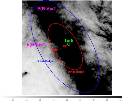
Figure 1.1: Reddening map of the central region of the Galaxy. Dark colors indicate large extinction, with color excess E(B-V)$>1$ dex and vice-versa. The location of Terzan 5 is marked in green, together with the extent of the outer bulge (blue ellipse) and of the inner bulge (red ellipse).

1.1 The structure of the Galactic bulge

The Galactic bulge is a triaxial, oblate system possibly composed of three bar structures: a central massive bar, a long thin bar, and a nuclear bar. While the presence of the first main component is well established, the existence of the other two, minor bars is still debated (see e.g. Gerhard & Martinez-Valpuesta 2012).

The main component is a boxy bar, that accounts for most of the mass of the bulge itself, being as massive as about $2\times 10^{10}$ M_⊙. Its presence has been traced with different methods, from the kinematics of gas (Liszt & Burton 1980) and planetary nebulae (Beaulieu et al. 2000), to star counts (e.g. Gonzalez et al. 2012) and optical depth gradients in microlensing events (Zhao & Mao 1996). The collected observables point toward the presence of a bar which is $\sim 2-3$ kpc in radius, with a vertical scale height of $\sim 300$ pc, an axis ratio of about $1:0.3:0.3$ and tilted by an angle of $\sim 20-30$°with respect to the line of sight (Babusiaux & Gilmore 2005; Cao et al. 2013). A sketch of the main bar structure is plotted in Figure 1.2.

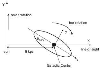
Figure 1.2: Shape and orientation of the main bar as it appears if the Galaxy is seen face-on. The near side of the bar is at positive Galactic longitude. The clockwise rotation of the bar is also marked (Figure taken from Rich 2013).

Recent IR observations demonstrated that the color-magnitude diagram (CMD) of bulge stars shows a double red clump (RC, see Figure 1.3), clearly separated in magnitude (McWilliam & Zoccali 2010; Nataf et al. 2010). This feature has been interpreted in terms of a distance effect, due to a X-shaped distribution of stars in the bar. According to this interpretation, the bar would show its X-shape when seen tangentially, while it appears boxy/peanut-shaped when viewed from the Sun.

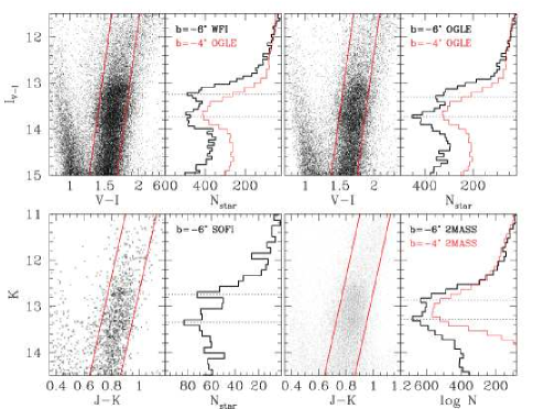
Figure 1.3: Optical (upper panels) and IR (lower panels) CMD of the bulge analyzed in McWilliam & Zoccali (2010). The luminosity functions for stars at Galactic latitude b$=-6$° (black histograms) clearly show two distinct peaks.

The stronger evidence for the presence of a “long bar”comes from an asymmetry in the disk star counts towards the Galactic center found by several authors (Hammersley et al. 2001; Benjamin et al. 2005). According to these works, such a long bar would be thin, with a vertical scale height of about $100$ pc, and seen with an inclination angle of 45°, thus almost aligned with the main bar. However, such an asymmetry has been observed only in the first quadrant, and its detection may be strongly biased by the presence of foreground disk stars. Therefore, accurate proper motion data are necessary to disentangle this sub-structure from the main bar and to firmly asses its actual existence.

An inner, nuclear bar has been also claimed, but its precise definition is more challenging, given both the strong extinction in the direction of the Galactic center and the contamination by the other sub-structures. According to Alard (2001), this bar should have an inclination angle of $\sim 70$°and may be as massive as the long bar.

Finally the presence of any spheroidal component, and the amount of bulge mass enclosed in it, is still debated. If we define the spheroidal component of the bulge as that formed either via hierarchical merging of substructures (Toomre 1977) or from the monolithic collapse of primordial gas clouds (Eggen et al. 1962), then such a component should be slowly rotating, mostly supported by random motions, and with surface brightness profiles following a Sersic law $\mu(r)\sim r^{1/n}$, with Sersic index $n\sim 4$. Recent kinematical observations (see Section 1.2.3) ruled out any spheroidal component contributing for more than the $8\%$ of the bulge mass (Shen et al. 2010). Moreover, measured values of the Sersic index are typically smaller, around 2-2.5 (Rich 2013), closer to what observed in the so-called pseudo-bulges (see Kormendy & Kennicutt 2004). However, numerical simulations by Saha et al. (2012) demonstrated that the buckling instability of the bar may have spun up any possible spheroidal component, which would therefore be kinematically indistinguishable from the bar at the present epoch.

1.2 Bulge stellar populations

In order to constrain the possible scenarios for the formation and evolution of the Galactic bulge, it is crucial to characterize its stellar populations in terms of age, chemistry and kinematics.

1.2.1 Age

The best way to determine the absolute age of a stellar population is by measuring the luminosity of the Main-Sequence Turn-Off (MSTO) in the CMD. The CMD of the Galactic bulge is particularly difficult to measure because of the strong contamination by disk field stars. When properly decontaminated by means of statistical star counts (as in Zoccali et al. 2003; Valenti et al. 2013) or by proper motions analysis (Clarkson et al. 2008, see Figure 1.4), the CMDs obtained in all the studies performed so far revealed that the bulge is predominantly old, at least as old as its globular clusters ($\gtrsim 10$ Gyr). Moreover, by considering also the population of Blue Straggler Stars (BSS) that in the CMD can mimic a younger component, Clarkson et al. (2011) concluded that only $<3.4$% of the bulge population can be younger than 5 Gyr.

The old age of the bulge is also confirmed by the discovery of RR Lyrae stars (e.g. Baade 1951; Alcock et al. 1998), which are good tracers of old stellar populations.

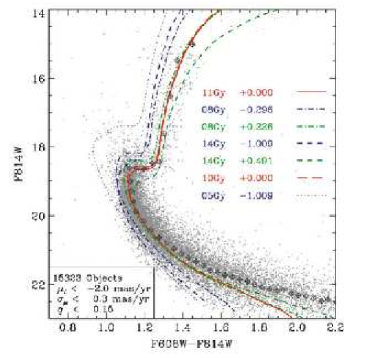
Figure 1.4: Proper-motion-selected optical CMD of the bulge stars in the Sagittarius I Field. The luminosity of the MSTO indicates that most of the population is old. The MS is in fact best-fitted by an 11 Gyr old isochrone, with very small room for satisfactory fits by younger models.

Although the bulk of the bulge is old, several pieces of evidence have been found supporting the presence of an intermediate-age population. This includes the discovery of long periods ($>400$ days) Mira variables, that are associated with younger ages (Feast 1963). However, a recent work on Mira variables (Blommaert & Groenewegen 2007) compiled from the Optical Gravitational Lensing Experiment II survey (OGLE-II, Udalski et al. 2000) concluded that the majority of these stars lie in the innermost 50 pc of the bulge.

Microlensing is a very powerful approach to study the faint population of bulge dwarfs. In fact, the strong magnification due to microlensing events can boost the magnitude of such stars by up to 5 mag, thus making them very good targets for medium-high resolution spectroscopy. From this kind of analysis, Bensby et al. (2013) found evidence for a quite large ($\sim 25$%) young and metal-rich stellar component (see Figure 1.5), numerically inconsistent with the results drawn from the CMD analysis. However, such studies are possibly affected by biases that favor the selection of metal-rich (and young) sources (Cohen et al. 2010). Also, the precise age of these stars depends on the adopted He-content (see e.g. Nataf & Gould 2012).

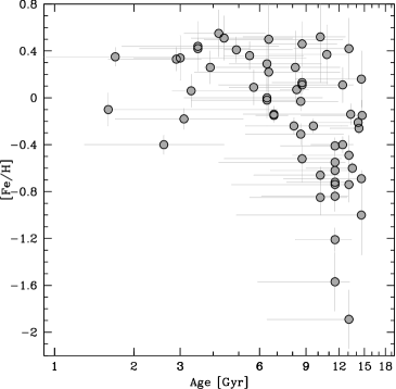
Figure 1.5: Age vs. metallicity relation for the sample of microlensed bulge dwarfs analyzed by Bensby et al. (2013). An important fraction of these stars ($\sim 25$%) appear to be younger than 6 Gyr.

Young and intermediate-age stellar populations are instead certainly present in the inner 100 pc of the bulge (Mezger et al. 1999; van Loon et al. 2003; Schuller et al. 2006).

1.2.2 Chemistry

The chemical composition of the Galactic bulge is a crucial information to constraint its formation and evolutionary history, and to understand its connection with other Galactic populations such as those in the disk and the halo.

The investigation of the bulge chemistry using medium and high-resolution spectroscopy started a few decades ago. McWilliam & Rich (1994) were the first to measure abundances for a large sample of K giants in the Baade’s Window from high signal-to-noise (SNR), optical spectra with resolution R$\sim 17000$. These authors found the iron abundances of bulge stars to span a wide range of values, from [Fe/H]$\sim-1$ dex to [Fe/H]$\sim+0.5$ dex. Moreover, they found the $\alpha$-elements to be enhanced relative to both the thick and the thin disk populations.

These two main features have been confirmed by many subsequent works. In fact, both optical (e.g. Fulbright et al. 2006; Zoccali et al. 2008; Johnson et al. 2011, 2012, 2013; Ness et al. 2013a; Johnson et al. 2014) and infrared (e.g. Rich & Origlia 2005; Rich et al. 2007; Rich, Origlia & Valenti 2012) studies, in different locations of the bulge, demonstrated that the metallicity distribution of its stars peaks around solar [Fe/H] (with a vertical gradient of about $-0.6$ dex kpc^-1, that likely flattens at latitudes $|b|<4$°), and reaches iron abundances as high as $\sim+0.5$ dex with a long metal-poor tail down to [Fe/H]$\sim-1.5$ dex (see for example Figure 1.6 taken from Zoccali et al. 2008).

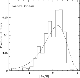
Figure 1.6: Metallicity distribution of the sample of bulge RC stars analyzed by Zoccali et al. (2008). The distribution peaks at solar values and displays a long metal-poor tail down to [Fe/H]$\sim-1.5$ dex, while reaching metallicity as high as [Fe/H]$\sim+0.5$ dex.

Some works found this metallicity distribution to be multi-modal (Hill et al. 2011; Ness et al. 2013a), with two main components peaking at sub-solar ([Fe/H]$\sim-0.3$ dex) and super-solar ([Fe/H]$\sim+0.3$ dex) metallicity. The $\alpha$-elements have generally been found to be enhanced with respect to iron at least up to solar [Fe/H] and then progressively declining towards solar values of [$\alpha$/Fe] (see Figure 1.7), with the location of the knee in the [$\alpha$/Fe] vs [Fe/H] trend possibly occuring at different metallicities depending on the kind of $\alpha$-element (Fulbright et al. 2007; Gonzalez et al. 2011). Such a behavior suggests that the stars with [Fe/H]$<0$ dex probably formed from a gas mainly enriched by core collapse supernovae (ccSN) on very short timescales and with a quite high star formation rate (SFR), while stars with super-solar metallicity probably formed from a gas further polluted by SNIa. Also, at odds with what is observed for iron abundances, no [$\alpha$/Fe] abundance gradient has been found in the bulge.

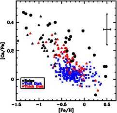
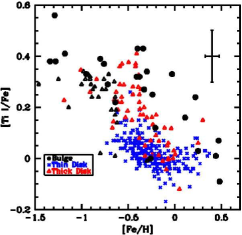
Figure 1.7: Examples of $\alpha$-enhancement for the sample of bulge stars (black dots) studied in Fulbright et al. (2007). The left panel shows the behavior of Calcium, while Titanium is plotted in the right panel. In both cases the differences among the bulge sample with respect to thin disk (blue crosses) and thick disk (red triangles) stars are evident, with the bulge sample being more enhanced and with the knee point being located at higher metallicity.

Given these abundance patterns, the bulge appears as a different population with respect to the thin/thick disk and the halo in many respects. First of all, the metallicity regime of the bulge is clearly much different with respect to that of the halo (see Figure 1.8). Moreover, the rare bulge stars at [Fe/H]$<-1.3$ dex, which somewhat overlap the metal-intermediate and poor halo populations, exhibit similar trends only in terms of “explosive” $\alpha$-elements (i.e. those produced during ccSN events, such as Ca, Si, Ti), but with a much smaller scatter than what is observed in halo stars (Fulbright et al. 2007, see Figure 1.8).

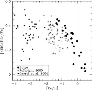
Figure 1.8: Summed abundances of the explosive $\alpha$-elements Si, Ca and Ti. The bulge stars (sample taken from Fulbright et al. 2007 and plotted as black filled circles) clearly shows a smaller scatter than halo stars (other symbols, from Fulbright 2000; Cayrel et al. 2004).

Secondly, the $\alpha$-element abundance pattern observed in the bulge is clearly different from that of the thin disk (which stays almost constant at solar values, see Figure 1.7), resulting from a more recent and prolongated star formation. Also, the light odd element Al is an efficient tool in separating these populations, as clearly demonstrated in Fulbright et al. (2007) where Al in bulge stars was found to be definitely enhanced with respect to both thin disk and dwarf galaxies (see Figure 1.9).

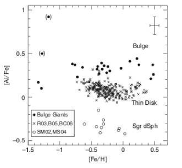
Figure 1.9: Comparison among [Al/Fe] vs [Fe/H] abundances for bulge, thin disk and dwarf galaxies stars. Bulge stars (black filled circles) are clearly over-abundant in Al content with respect to the other samples.

Finally, the separation between bulge and thick disk stars in terms of $\alpha$-elements is less neat and still disputed. Several works found the bulge giants to be more enhanced than thick disk giants. This has also been confirmed for a sample of microlensed dwarf stars by Bensby et al. (2013). Only Meléndez et al. (2008); Ryde et al. (2009) and Alves-Brito et al. (2010) claim no or small differences between these two populations, especially in the [O/Fe] trend, but their samples are smaller and less statistically significant. An important difference has been found when measuring heavy neutron-capture element abundances, such as La and Eu. In fact, bulge stars have low [La/Eu] over almost the entire range of metallicities (pure r-process regime, see Kappeler et al. 1989), this being consistent with a so fast enrichment that AGB stars had not enough time to pollute the star-forming gas with s-process (see the upper panel of Figure 1.10 from Johnson et al. 2012). Instead, the thick disk has an higher [La/Eu], more compatible with a gas s-process polluted on longer timescales.

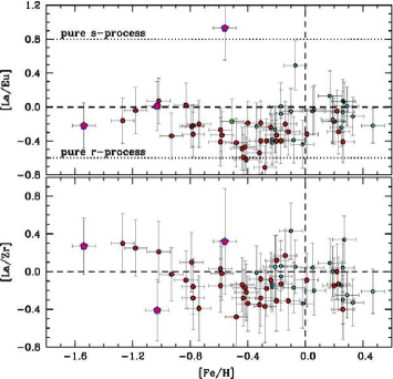
Figure 1.10: Upper panel: [La/Eu] vs. [Fe/H] for the bulge stars analyzed in Johnson et al. (2012). Red giant branch (RGB) stars are plotted in red, while RC stars are shown as cyan circles. The level of [La/Eu] is consistent with a pure r-process regime, indicating an extremely fast enrichment.

1.2.3 Kinematics

The first studies of the bulge kinematics used neutral hydrogen (HI) gas as a tracer (Liszt & Burton 1980). From these works the first evidence of the presence of a bar was obtained (see Section 1.1), with structural parameters close to those favored today (Binney et al. 1991). Stellar tracers have been systematically used only later on, when multi-object spectrographs became available to the community, allowing the measure of radial velocity for large samples of bulge stars.

In the recent years, two major radial velocity surveys of the outer bulge have been undertaken.

($1$) The Bulge RAdial Velocity Assay (BRAVA, Rich et al. 2007) measured radial velocity for $4500$ M giants located between $-10$°$<$l$<10$°and $-8$°$<$b$<-4$°, finding that the bulge does not show a pure solid-body rotation but exhibits a cylindrical rotation (Howard et al. 2008, 2009; Kunder et al. 2012, see Figure 1.11).

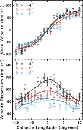
Figure 1.11: Radial velocity (upper panel) and velocity dispersion (lower panel) vs. Galactic longitude trends for the bulge fields studied in the BRAVA survey. The different colors indicate different Galactic latitudes. The typical features of cylindrical rotation are evident in both cases.

According to these results, Shen et al. (2010) demonstrated using N-body simulations that the fraction of the bulge component in a non-barred configuration should be smaller than the 8%.

($2$) The Abundance and Radial velocity Galactic Origins Survey (ARGOS, Freeman et al. 2013) targeted more than $28000$ stars in the bulge and in the inner disk measuring both radial velocity and chemical abundances and found a rotation curve in good agreement with the BRAVA results (see Figure 1.12).

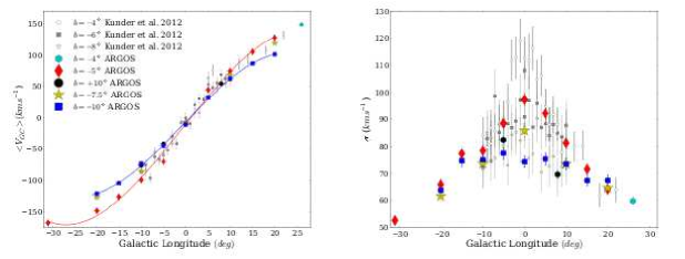
Figure 1.12: Same plots as in Figure 1.11 but for the bulge fields surveyed by ARGOS. The results of this survey (shown with different colored symbols depending on the latitude) agree well with the BRAVA results (shown as grey symbols).

Very recently the Giraffe Inner Bulge Survey (GIBS, Zoccali et al. 2014) has been carried out with the aim of measuring radial velocities and chemical abundances for about $6500$ RC stars in the inner bulge. The first results of the survey confirm the cylindrical rotation of the bulge also for a sample of K giants at Galactic latitude b$=-2$°, in a region closer to the Galactic plane than probed by the previous surveys, and found a velocity dispersion peak in the bulge central region, possibly indicating the presence of an overdensity in the inner $250$ pc (see Figure 1.13).

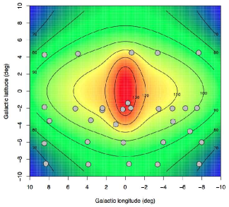
Figure 1.13: Color-coded velocity dispersion map obtained by the GIBS survey. A high velocity dispersion peak is evident in the central region of the bulge, possibly indicating the presence of an over-density in the inner 250 pc of the Galaxy.

Other powerful approaches to study the kinematics of the bulge are the Fabry-Perot imaging in the Ca II 8542 absorption line (see Rangwala et al. 2009) and proper motions. In fact, the typical peak velocity dispersion of the bulge (of the order of $\sim 100$ km s^-1) correspond to 2-3 ${\rm mas\,yr^{-1}}$in terms of proper motions. Such a value is measurable in reasonable temporal baselines also with ground-based observations. By using data from the OGLE-II survey, Rattenbury et al. (2007) found that the proper-motion dispersion of bulge stars declines with increasing Galactic latitude and longitude.

Also, by combining radial velocity and proper motions it is possible to build the so-called velocity ellipsoid. Zhao et al. (1994) found that for bulge stars a correlation between transverse proper motion and radial velocity exists. This produces a velocity ellipsoid with a major axis which appears angled off of normal (see Figure 1.15). Such a feature is called vertex deviation and appears to be related to stars with bar-like orbits (Zhao & Mao 1996; Soto et al. 2007).

The combination of chemical and kinematical information gives other important clues to understand the complexity of the bulge populations. Ness et al. (2013b) decomposed the metallicity distribution of the bulge in several Gaussian components and distinguished two main populations with a rotating bar kinematics, one peaking at [Fe/H]$\simeq-0.25$ dex and being $\alpha$-enhanced and the other peaking at [Fe/H]$\simeq+0.15$ and kinematically colder. On the other hand, they found only a small fraction (5%) of metal-poor stars ([Fe/H]$<-1$ dex) showing a kinematics typical of a slowly rotating spheroidal, with a velocity dispersion not changing with longitude. These kinematical features for the three components are summarized in Figure 1.14, where both the rotation curve and the velocity dispersion trend with respect to the Galactic longitude are shown (different colors represent samples at different Galactic latitude).

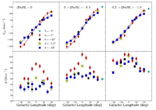
Figure 1.14: Same plots as in Figure 1.12 but for three different bins of metallicity. The sub and super-solar components (left and middle panels) show the same behavior, with the typical features of cylindrical rotation. On the other end, the most metal-poor component (right panel) shows a kinematic more compatible with that of a slowly rotating spheroidal.

Finally, Zhao et al. (1994); Soto et al. (2007); Babusiaux et al. (2010) observed a vertex deviation in the velocity ellipsoid only for stars with [Fe/H]$>-0.5$ dex (see Figure 1.15), thus indicating that most of the bar population should be more metal-rich than this value.

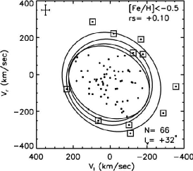
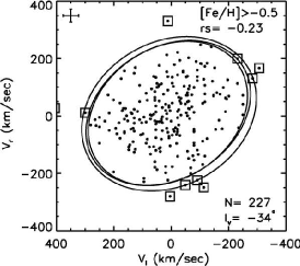
Figure 1.15: Example of vertex deviation (from Soto et al. 2007). In the left panel, stars with [Fe/H]$<-0.5$ dex do not show evidence of correlation among the velocity ellipsoid components. In the right panel, stars with [Fe/H]$>-0.5$ dex display a correlation between radial velocity and the transverse component of proper motion. This causes the velocity ellipsoid to have a preferential orientation which is defined as vertex deviation.

1.3 Bulge formation and evolution theories

The old age of the bulge stars and the observed chemical patterns indicate that the bulge formed early and rapidly, from a gas mainly enriched by ccSN (Matteucci & Brocato 1990; Matteucci & Romano 1999). Chemical evolutionary models have been able to reproduce the observed chemistry by requiring a formation timescale smaller than 1 Gyr (Ballero et al. 2007; Cescutti & Matteucci 2011). Such properties, together with the presence of a vertical abundance gradient, are naturally accounted for by a dissipative collapse model (Eggen et al. 1962).

On the other hand the stellar kinematics of the bulge, which appears peanut/X-shaped and which is cylindrically rotating, is consistent with a purely dynamical evolution of a disk buckling into a bar (Shen et al. 2010; Saha et al. 2012). However, these authors argued that the presence of a bar would have spun up to cylindrical rotation any classical bulge component, thus making it kinematically indistinguishable. Martinez-Valpuesta & Gerhard (2013) demonstrated that a bulge formed from the instability of the disk would show a vertical abundance gradient if the original disk were characterized by a radial abundance gradient.

Another interesting hypothesis (see e.g. Immeli et al. 2004; Carollo et al. 2007; Elmegreen et al. 2008) is that bulges form at high redshift (z$\sim 2-3$) via a combination of disk instabilities and mergers of giant clumps (Elmegreen et al. 2008; Dekel et al. 2009) on short dynamical timescales. These giant clumps would form stars rapidly and with very high SFR (thus producing stars that today would appear old and with the same chemistry as that observed in the bulge) and then would dynamically evolve towards the center of the galaxy. There, they would merge together and their stars would develop the typical kinematics of a bar.

The only way to directly test this latter scenario is to find the relics of such massive clumps, which may still be orbiting in the bulge of the host galaxy. Ferraro et al. (2009, hereafter F09) may have discovered the first remnant of one of these objects in our Galaxy: the bulge stellar system Terzan 5.

1.4 Terzan 5

Terzan 5 is a stellar system commonly catalogued as an old (Ortolani et al. 2001) globular cluster (GC), located in the bulge of our Galaxy (its Galactic coordinates are $l=3.8395$°, $b=1.6868$°). The distance (5.9 kpc, see also Ortolani et al. 2007) and reddening (E(B-V)$=2.38$, see also Barbuy et al. 1998) we adopt in this Thesis are from Valenti et al. (2007) F09 discovered the presence of two distinct sub-populations, which define two RCs clearly separated in luminosity and color in the $(K,J-K)$ CMD (Figure 1.16) obtained through observations taken with the Multi-Conjugate Adaptive Optics Demonstrator (MAD) mounted at the Very Large Telescope (VLT).

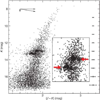
Figure 1.16: IR CMD of Terzan 5. The inset highlights the presence of the two RCs, well separated in color and magnitude, in a direction perpendicular to that of the reddening vector (shown as a black arrow in the top-left corner of the Figure). Photometric errors are also marked on the right side of the plot.

The analysis of high-resolution IR spectra obtained with NIRSPEC at the Keck II telescope, demonstrated that the two populations have significantly different iron content (see the left panel of Figure 1.17): the bright RC (at $K=12.85$) is populated by a quite metal rich component ([Fe/H]$\simeq+0.3$), while the faint clump (at $K=13.15$) corresponds to a relatively metal poor population at [Fe/H]$\simeq-0.2$. Before this discovery, such a large difference in the iron content ($\Delta$ [Fe/H]$>0.5$ dex) was found only in $\omega$ Centauri, a GC-like system in the Galactic halo, now believed to be the remnant of a dwarf galaxy accreted by the Milky Way.

Figure 1.17: Left panel: Combined spectra measured for three faint RC (FHB) and three bright RC (BHB) stars in Terzan 5. Solid lines correspond to the best-fit synthetic spectra computes at the marked metallicities ([Fe/H]$\simeq-0.2$ dex and [Fe/H]$\simeq+0.3$ dex). The dashed lines show the spectra expected by assuming the reverse metallicities ([Fe/H]$\simeq 0.3$ dex for the FHB and [Fe/H]$\simeq-0.2$ dex for the BHB). Right panel: isochrone fitting of the IR CMD of Terzan 5. The metal-poor component is best fitted with an old ($12$ Gyr) isochrone, while the metal-rich population is well fitted by a younger isochrone ($6$ Gyr old). All the theoretical models are taken from the BaSTI database (Pietrinferni et al. 2004, 2006).

Origlia et al. (2011, hereafter O11) presented a detailed study of the abundance patterns of Terzan 5, demonstrating that (1) the abundances of light elements (like O, Mg, and Al) measured in both the sub-populations do not follow the typical anti-correlations observed in genuine GCs (Carretta et al. 2009; Mucciarelli et al. 2009, see left panel of Figure 1.18); (2) the overall iron abundance and the $\alpha-$enhancement of the metal poor component demonstrate that it formed from a gas mainly enriched by Type II supernovae (SNII) on a short timescale, while the progenitor gas of the metal rich component was further polluted by SNIa on longer timescales; (3) these chemical patterns are strikingly similar to those measured in the bulge field stars (see the right panel of Figure 1.18), with the $\alpha$-elements being enhanced up to solar metallicity and then progressively decreasing towards solar values (see Section 1.2.2).

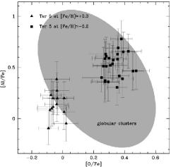
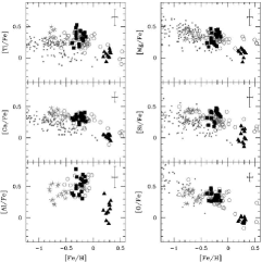
Figure 1.18: Spectroscopic screening of Terzan 5 giants from Origlia et al. (2011). Left panel: the light elements measured in Terzan 5 stars (solid circles and triangles) clearly do not show the typical anti-correlation commonly observed in genuine GCs (the grey shaded area). Right panel: all the measured $\alpha$-elements for Terzan 5 targets (black filled symbols) follow the same trend observed for bulge stars (grey symbols) in the [$\alpha$/Fe] vs [Fe/H] plot.

There is also another interesting chemical similarity between Terzan 5 and the bulge stellar population. In fact, as already described in Section 1.2.2, the latter shows a metallicity distribution with two major peaks at sub-Solar and super-Solar [Fe/H], very similar to the metallicities of the two populations discovered in Terzan 5. Chemical abundances of bulge dwarf stars from microlensing experiments (see e.g. Cohen et al., 2010; Bensby et al., 2013, and references therein) also suggest the presence of two populations, a sub-Solar and old one with [$\alpha$/Fe] enhancement, and a possibly younger, more metal-rich one with decreasing [$\alpha$/Fe] enhancement for increasing [Fe/H].

Each Terzan 5 component shows a small internal metallicity spread and the most metal-rich population is also more centrally concentrated (F09, Lanzoni et al. 2010, hereafter L10).

All these observational results demonstrate that Terzan 5 is not a genuine GC, but a stellar system with a more complex star formation and chemical enrichment history. Indeed it is likely to have been much more massive in the past than today (with a mass of at least a few $10^{7}-10^{8}M_{\odot}$, while its current value is $\sim 10^{6}M_{\odot}$; L10), thus to retain the high-velocity gas ejected by violent SN explosions. Moreover, it likely formed and evolved in strict connection with its present-day environment (the bulge), thus suggesting the possibility that it is the relic of one of the pristine fragments that contributed to form the Galactic bulge itself. In this context, also the extraordinary population of millisecond pulsars (MSPs) observed in Terzan 5 can find a natural explanation. In fact, the system hosts 34 MSPs. This amounts to $\sim 25\%$ of the entire sample of MSPs known to date in Galactic GCs (Ransom et al., 2005, ; see the updated list at www.naic.edu/$\sim$pfreire/GCpsr.html). In order to account for the observed chemical abundance patterns, a large number of SNII is required. These SNII are expected to have produced a large population of neutron stars, mostly retained by the deep potential well of the massive proto-Terzan 5. The large collisional rate of this system (Verbunt & Hut, L10) may also have favored the formation of binary systems containing neutron stars and promoted the re-cycling process responsible for the production of the large MSP population now observed in Terzan 5.

Chapter 2 HST Relative Proper Motions of Terzan 5

As already discussed in Chapter 1, the analysis of the evolutionary sequences in the optical CMD of Terzan 5 is extremely difficult because of the large differential extinction and the strong contamination of the underlying bulge population and foreground sources.

In this Chapter the issue of field contamination is addressed. In general, the most efficient way to decontaminate CMDs from non-member stars is the determination of accurate stellar proper motions (PMs). To this aim, we analyzed two epochs of high-resolution Hubble Space Telescope (HST) images obtaining relative PMs (i.e. PMs of stars in the HST field of view with respect to the average motion of Terzan 5) for more than $100,000$ stars reaching m${}_{{\rm F606W}}\simeq 28$, i.e. about 3 magnitudes below the MSTO. This allowed us to define a method to reliably select cluster member stars and discard foreground and background sources.

Two additional applications of the technique used in this Thesis are also presented in the Appendix.

2.1 Observations

In order to measure the PMs in the direction of Terzan 5 we used two HST high-resolution data sets acquired with the Wide Field Channel (WFC) of the Advanced Camera for Survey (ACS). The WFC/ACS is made up of two $2048\times 4096$ pixel detectors with a pixel scale of $\sim 0.05\mbox{${}^{\prime\prime}$}\,$pixel^-1 and separated by a gap of about 50 pixels, for a total field of view (FoV) of $\sim 200\mbox{${}^{\prime\prime}$}\times 200\mbox{${}^{\prime\prime}$}$. The data set used as first epoch was obtained under GO-9799 (PI: Rich). It consists of two deep exposure images, one in the F606W filter and the other in the F814W filter (with exposure times of $340$ s), and one short exposure ($10$ s) image in the F814W filter, taken on September 9, 2003.

The second-epoch data set is composed of data obtained through GO-12933 (PI: Ferraro). This program consists of several deep images taken both with the WFC/ACS in the F606W and F814W filters, and with the IR channel of the Wide Field Camera 3 (WFC3) in the F110W and F160W filters. The WFC3 IR camera is made of a single $1024\times 1024$ pixel detector. Its pixel scale is $\sim 0.13\mbox{${}^{\prime\prime}$}\,$pixel^-1 and the total FoV is $123\mbox{${}^{\prime\prime}$}\times 136\mbox{${}^{\prime\prime}$}$. Because of the larger pixel size of the WFC3 IR detector (it is almost three time the size of the WFC/ACS pixel) and given that the Full Width Half Maximum (FWHM) of the Point Spread Function (PSF) in the IR is larger than in the optical bands, we used only the WFC/ACS images for the PM determination. The sample used consists of $5\times 365\,$s images in F606W and $5\times 365\,$s images in F814W, with one short exposure image per filter ($50$ s and $10$ s, respectively). These observations were taken on August 18, 2013, therefore the two available data sets provide a temporal baseline of $\sim 9.927$ yrs.

2.2 Relative Proper Motions

The techniques applied in the present work have been developed in the context of the HSTPROMO collaboration (van der Marel et al. 2014; Bellini et al. 2014), of which I am currently member. HSTPROMO aims at improving our understanding of the dynamical evolution of stars, stellar clusters and galaxies in the nearby Universe through measurement and interpretation of proper motions.

The analysis has been performed on _FLC images, which have been flat-fielded, bias-subtracted and corrected for Charge Transfer Efficiency (CTE) losses by the pre-reduction pipeline with the pixel-based correction described in Anderson & Bedin (2010) and Ubeda & Anderson (2012). The main data-reduction procedures we used are described in detail in Anderson & King (2006). Here we provide only a brief description of the main steps of the analysis. The first step consists in the photometric reduction of each individual exposure of the two epochs with the publicly available program img2xym$\_$WFC.09$\times$10. This program uses a pre-determined model of spatially varying PSFs plus a single time-dependent perturbation PSF (to account for focus changes or spacecraft breathing). The final output is a catalog with instrumental positions and magnitudes for a sample of sources above a given flux threshold in each exposure. Star positions were then corrected in each catalog for geometric distortion, by means of the solution provided by Anderson (2007).

To check the quality of our photometry, we built the WFC/ACS (m_F606W, m${}_{{\rm F606W}}-$m_F814W) CMD of Terzan 5. The F606W and the F814W samples were constructed by selecting stars in common among at least 3 out of 5 deep-single-exposure catalogs. The CMD resulting from these two samples is shown in Figure 2.1. The instrumental magnitudes have been calibrated onto the VEGAMAG system using aperture corrections and zeropoints reported in the WFC3 web page. As it is evident from Figure 2.1, the evolutionary sequences of Terzan 5 are strongly affected by differential reddening, however they can be identified well in the CMD obtained. The MS extends for almost $4$ magnitudes below the TO. A blue sequence is visible at m${}_{{\rm F606W}}<23$ mag and (m${}_{{\rm F606W}}-$m${}_{{\rm F814W}})<2.6$ mag and it remains well separated from the cluster RGB. This sequence is likely populated by young field stars.

Figure 2.1: (m_F606W, m${}_{{\rm F606W}}-$m_F814W) CMD of Terzan 5. All the cluster evolutionary sequences are distorted because of differential reddening effect. A bright, blue sequence is clearly separated from the cluster sequences and it is likely traced by young field stars.

The second step in measuring relative PMs is to astrometrically relate each exposure to a distortion-free reference frame, which from now on we will refer to as the master frame. Since no high-resolution photometry other than that coming from these data sets is available, we defined as master frame the catalog obtained from the combination of all the second-epoch single-exposure catalogs corrected for geometric distortions. In this way, the master frame is composed only of stars with at least $10$ position measurements (5 for each filter). We then applied a counter-clockwise rotation of $88.84$°  in order to give to the master frame the same orientation as the absolute reference frame, here defined by the Two Micron All Sky Survey (2MASS) catalog (see L10).

We then transformed the measured position of each star in each exposure into the master frame by means of a six-parameter linear transformation based on the positions of several hundreds reference stars. Such reference stars are the stars with respect to which our PMs would be computed. For convenience, we chose to compute all PMs relative to the mean motion of the cluster. Therefore our reference list is composed of stars which are likely cluster members. These are initially selected on the basis of their location on the CMD, including in the list only well-measured and unsaturated stars. Then, for each star in each catalog, we computed the position on the master frame using a transformation based on only the closest 50 reference stars. To maximize the accuracy of these transformations we treated each chip of our exposures separately, in order to avoid spurious effects related to the presence of the gap.

Figure 2.2: Uncertainties in the X and Y displacements in units of pixel yr^-1. Bright, well measured stars have displacement errors typically smaller than 0.002 pixel yr^-1 in each coordinate, i.e. smaller than 0.1 ${\rm mas\,yr^{-1}}$.

At the end of the procedure, for each star we have up to $3$ first-epoch position measurements and up to $12$ second-epoch positions on the master frame. However, stars brighter than m${}_{{\rm F606W}}\simeq 17.9$ saturate in the long exposures. Therefore, for the brightest stars we have only $1$ first-epoch and $2$ second epoch positions. To estimate the relative motion of each star we adopted a 3$\sigma$-clipping algorithm and computed the median X and Y positions of each star in the first and in the second epoch. The difference between the two median positions gives the star’s X and Y displacements in $\Delta{\rm T}=9.927$ years. To determine the displacements of bright stars with only one or two positional measurements, we adopted either the single or the mean X and Y position values, respectively. The errors in each direction and within each epoch ($\sigma_{1,2}^{{\rm X,Y}}$) were computed as:

$${\rm rms_{1,2}^{{\rm X,Y}}}/\sqrt{N_{1,2}}$$ (2.1)

where rms_1,2 is the rms of the positional residuals about the median value, and N_1,2 is the number of measurements. Therefore, the error in each PM-component associated to each star is simply the sum in quadrature between first- and second-epoch errors: $\sigma_{\rm PM}^{{\rm X}}=\sqrt{(\sigma_{1}^{{\rm X}})^{2}+(\sigma_{2}^{{\rm X}})^{2}}/\Delta{\rm T}$ and $\sigma_{\rm PM}^{{\rm Y}}=\sqrt{(\sigma_{1}^{{\rm Y}})^{2}+(\sigma_{2}^{{\rm Y}})^{2}}/\Delta{\rm T}$. The error associated to the PM of the brightest stars measured only in the short exposures were computed by adopting as positional uncertainties the typical errors determined in the long exposure catalogs at the same instrumental magnitude.

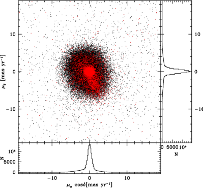
Figure 2.3: Vector Point Diagram (VPD) of the PMs measured for the $127,172$ stars (black dots) in the direction of Terzan 5. Their distributions in the Right Ascension and Declination axis are shown in the histograms in the bottom and right panel, respectively. PMs measured for stars with m${}_{F606W}<24$ mag are shown as red dots. At least two components are visible: the first showing a symmetric distribution centered around the origin (corresponding to the bulk of Terzan 5 member stars) and an asymmetric structure roughly centered at (2.5, -5) ${\rm mas\,yr^{-1}}$.

By selecting stars on the basis of this first PM determination, we repeated the entire procedure the number of times needed to make the number of stars in the reference list stable, i.e. with variations smaller than 2-3%. To be conservative, for all the unsaturated stars in the deep exposures we decided to build the final PM catalog taking into account only the 123 172 stars having at least 2 position measurements in each epoch. The typical error as a function of magnitude is shown in Figure  2.2. For well-exposed stars it is smaller than 0.002 pixel yr^-1 in each coordinate, i.e. smaller than 0.1 ${\rm mas\,yr^{-1}}$. Faint stars or stars with only few epochs measurements show larger errors, but always smaller than 0.01 pixel yr^-1.

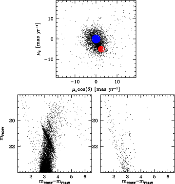
Figure 2.4: Upper panel: VPD of the stars brighter than m${}_{F606W}=24$ mag. Stars belonging to the symmetric component of likely members are plotted in blue, while those belonging to the asymmetric component centered at (2.5, -5) ${\rm mas\,yr^{-1}}$are plotted in red. Left-lower panel: CMD described by VPD-selected likely member stars. with the exception of few contaminating stars, only the cluster evolutionary sequences are visible. Right-lower panel: CMD described by stars belonging to the VPD asymmetric feature. This population is dominated by young foreground disk stars along the blue plum.

We converted the PMs into absolute units (${\rm mas\,yr^{-1}}$) by multiplying the measured displacements by the pixel scale of the master frame ($0.05\mbox{${}^{\prime\prime}$}/$pixel) and dividing by the temporal baseline ($9.927$ yr). Since the master frame is already oriented according to the equatorial coordinate system, the X PM-component corresponds to that projected along (negative) Right Ascension ($-\mu_{\alpha}\cos\delta$), while the Y PM-component corresponds to that along Declination ($\mu_{\delta}$). The output of this analysis is summarized in Figure 2.3, where we show the Vector Point Diagram (VPD) for all the stars with a measured PM.

By selecting stars with m${}_{{\rm F606W}}<24$ (red points in Figure 2.3), which typically have the most accurate PMs (red points in Figure 2.2), the VPD clearly shows at least two components. One is a symmetric distribution centered around the origin, corresponding to Terzan 5 member stars. The bulk of this population is confined within a circle of radius 2${\rm mas\,yr^{-1}}$. The other is an asymmetric structure approximately centered around the coordinate (2.5, -5) ${\rm mas\,yr^{-1}}$in the VPD. The location of these two components in the CMD clearly reveal their nature (see Figure 2.4). In fact, while the stars of the first component (shown as blue dots in the VPD) describe in the CMD the evolutionary sequences of the cluster (left-lower panel), the stars belonging to the asymmetric component (red dots) correspond in the CMD to the blue plum (right-lower panel) essentially populated by young disk stars in the foreground of Terzan 5.

Such a conclusion is confirmed by the comparison with the prediction of the Besançon model (Robin et al. 2003) for a field centered at the coordinates of Terzan 5 and having the same size as that of the WFC/ACS and with only young (t${}_{age}<7$ Gyr) Galactic disk stars (see Figure 2.5).

Figure 2.5: Comparison between the ACS optical CMD and that predicted by a simulation of the Besançon model including only Galactic disk stars younger than 7 Gyr. Such a comparison clearly demonstrates that the bluer sequence in the CMD of Terzan 5, already identified as composed of field stars by the PMs, correspond to the MS of foreground Disk stars.

2.3 Analysis of the PM-selected CMD

In this Section we analyze the CMDs obtained with different data sets and filters after an appropriate decontamination from non-member stars performed on the basis of the measured PMs.

2.3.1 Optical CMD

The first analysis is performed on the optical (m_F606W, m${}_{{\rm F606W}}-$m_F814W) CMD of Terzan 5 obtained with the WFC/ACS dataset described in Section 2.1. Since, as shown in Figure 2.3, the bulk of the PMs in the VPD is concentrated within a circle of radius $2$ ${\rm mas\,yr^{-1}}$and we expect it to be dominated by likely member stars, we adopted this as member selection criterium. We therefore considered all the sources lying outside such a circle as non-member stars. The CMD obtained from such a selection is shown in Figure 2.6.

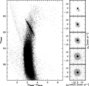
Figure 2.6: Left panel: optical CMD of Terzan 5. Stars selected as likely members are shown as black dots, while sources excluded by the selection are plotted in grey. The measured relative PMs are efficient in decontaminating the CMD and only cluster evolutionary sequences survive the selection criterium. Right panels: magnitude-binned VPDs for all the stars in the optical catalogue. Each bin has a size of 2 mag. Sources are color coded as in the left panel, and the red circles mark the selection of asymmetric feature.

In the Figure, member stars are plotted as black dots, while non members stars are shown in grey. The selection applied leaves in the CMD only stars clearly belonging to the cluster evolutionary sequences while excluding most of the outliers. A small degree of contamination is still present, probably because the distribution of field stars (mainly bulge stars) in the VPD overlaps that of Terzan 5 members. However, we can conclude that the PMs analysis performed in this Thesis is efficient in decontaminating the CMD from foreground and background sources in Terzan 5.

Since the method described to identify and reject foreground and background stellar sources in the direction of Terzan 5 is reliable and works well, in the following we will analyze the IR CMD obtained in F09 by means of observations taken with the MAD camera in order to check whether all the properties discovered in that CMD hold after the PM decontamination.

2.3.2 MAD Infrared CMD

With the aim of studying the large population of MSPs hosted by Terzan 5, F09 exploited the great capability of the multi-conjugate adaptive optics system MAD mounted at the VLT. The obtained (K, J-K) IR CMD revealed the presence of two well separated RCs (see Chapter 1). Since their separation in both color and magnitude is perpendicular with respect to the direction of the reddening vector, it has been interpreted as a genuine feature due to the presence of two sub-populations with different properties in terms of age, metallicity or helium content. A prompt spectroscopic follow-up demonstrated that the two populations have at least different metallicities, with stars belonging to the faint RC having [Fe/H]$\simeq-0.3$ dex and those belonging to the bright RC with [Fe/H]$\simeq+0.3$.

This spectroscopic follow-up also revealed that the samples of stars belonging to the two RCs have the same radial velocity, corresponding to the systemic velocity of Terzan 5. Moreover, the photometric study performed in L10 showed that the two RCs also share the same center of gravity. Finally, the bright RC was also found to be more centrally concentrated than the faint RC. All these findings clearly suggest that the two populations are members of Terzan 5 and exclude that they are the result of a superposition in the sky (in this case the bright RC should be the closer and thus less concentrated population, at odds with what is observed).

Despite this evidence, the membership of the two populations has been questioned in some works (see for example Willman & Strader 2012). To solve this issue, our PM analysis is applied to the IR CMD. The result is summarized in Figure 2.7.

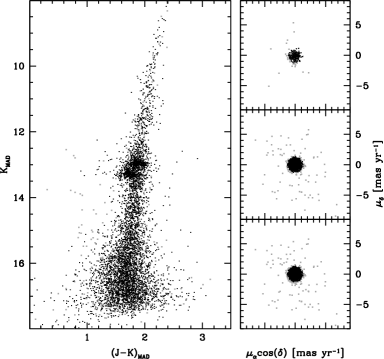
Figure 2.7: Left panel: IR CMD of Terzan 5 obtained from MAD observations. The PM-selected member stars are shown as black dots, while the sources excluded as grey dots. Despite the stringent selection, the presence of the two RC is evident. Right panels: magnitude-binned VPDs (each magnitude bin has a size of 3 mag). Stars are color-coded as in the left panel.

The left panel shows the IR CMD of Terzan 5 after the decontamination (black dots), with the sources excluded by the PM selection shown as grey dots. Such a selection is even more stringent in this case than that adopted in Section 2.3.1. In fact, as shown in the magnitude-binned VPDs in the right panels, we excluded all the stars with a total PM vector $\mu=\sqrt{(\mu_{\alpha}\cos\delta)^{2}+(\mu_{\delta})^{2}}>1.3$ ${\rm mas\,yr^{-1}}$. The overall smaller dispersion should not be interpreted as an intrinsic feature but rather as due to the fact that the IR CMD is less deep than the optical one and faint stars with more uncertain PM are not present. Despite such a tighter selection, the decontaminated CMD clearly exhibits the two well separated RCs.

Figure 2.8 shows the VPDs of stars properly selected in the two RCs. As can be seen, the two distributions appear quite symmetric, both showing a small (1.3${\rm mas\,yr^{-1}}$) dispersion around the origin. However we underline that the accuracy of these PMs is not sufficient to reveal possible intrinsic differences in the kinematics of the two populations. At this stage, we can only conclude that they are not distinguishable in terms of cluster membership, being both well within the adopted VPD-members selection criterium.

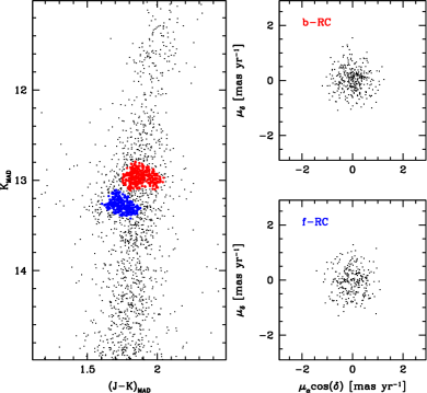
Figure 2.8: Left panel: IR-MAD CMD of Terzan 5 zoomed in the RC region. Faint-RC stars are plotted in blue, while bright-RC stars are plotted in red. Right panels: VPDs of b-RC (upper panel) and f-RC (lower panel) stars: in both cases stars lie within the 2${\rm mas\,yr^{-1}}$circle adopted as membership selection criterium. No clearcut differences between the two distributions are visible.

Overall the number of contaminants in the IR CMD is much smaller than what observed in the optical case. However this is somehow expected, given that this photometry comes from a smaller FoV in the very central region of the system, where the cluster population is supposed to dominate.

Therefore, the relative PMs measured in this Chapter and applied to the MAD CMD definitely demonstrate that both the populations discovered in Terzan 5 are clearly member of the system.

2.4 Conclusions

In this Chapter we addressed the issue of field contamination in the photometric analysis of Terzan 5. We performed a relative PM analysis to separate fore- and background stars from those belonging to the system. In particular, we used the approach developed in the context of the HSTPROMO collaboration to measure relative PMs for 123 172 optical sources found in the direction of Terzan 5.

The resulting VPD shows a dominant component distributed symmetrically around the origin of the diagram and extending out to about $2$ ${\rm mas\,yr^{-1}}$, and two minor and sparser components, one of them being clearly asymmetric and preferentially located in the fourth quadrant.

From the analysis of the optical CMD, we demonstrated that the measured PMs are efficient in decontaminating the photometry from non-member populations, and by comparing our photometry with that predicted by the Besançon model at the Terzan 5 coordinates we showed that the asymmetric feature observed in the VPD is likely to be populated by young Galactic disk stars.

Finally, the analysis of the PM-selected IR CMD showed that the two populations discovered in Terzan 5 are present in the CMD even after a stringent decontamination. Such an evidence, coupled with the features already discovered in previous works, demonstrates that both the populations in Terzan 5 are genuine members of the system.

Chapter 3 High resolution reddening map in the direction of the stellar system Terzan 5

Severe limitations to a detailed analysis of the evolutionary sequences in the CMDs of Terzan 5 are introduced by the presence of large differential reddening. To face this problem we build the highest-resolution extinction map ever constructed in the direction of this system. This is the subject of the present Chapter.

In particular, we used optical images acquired with the HST to construct an extinction map in the direction of Terzan 5 which has a spatial resolution of $8\mbox{${}^{\prime\prime}$}\times 8\mbox{${}^{\prime\prime}$}$, over a total FoV of $200\mbox{${}^{\prime\prime}$}\times 200\mbox{${}^{\prime\prime}$}$. The absorption clouds show a patchy structure on a typical scale of $20\mbox{${}^{\prime\prime}$}$ and extinction variations as large as $\delta E(B-V)\sim 0.67$ mag. These correspond to an absolute color excess ranging from $E(B-V)=2.15$ mag, up to 2.82 mag. After the correction for differential reddening, two distinct red giant branches become clearly visible in the optical color magnitude diagram of Terzan 5 and we verified that they well correspond to the two sub-populations with different iron abundances recently discovered in this system.

All the details of this study are described in Massari et al. (2012).

3.1 Differential reddening correction

3.1.1 The data-set

The photometric data used in this work consist of a set of high-resolution images obtained with the WFC of the ACS on board the HST (GO-9799, see F09 and L10). The WFC/ACS camera has a FoV of $\sim 200\mbox{${}^{\prime\prime}$}\times 200\mbox{${}^{\prime\prime}$}$ with a plate-scale of 0.05^′′/pixel. Both F606W (hereafter $V$) and F814W ($I$) magnitudes are available for a sample of about 127,000 stars. The magnitudes were calibrated on the VEGAMAG photometric system by using the prescriptions and zero points by Sirianni et al. (2005). The final catalog was placed onto the 2MASS absolute astrometric system by following the standard procedure discussed in previous works (e.g., L10). The $(I,V-I)$ CMD shown in Figure 3.1 clearly demonstrates the difficulty of studying the evolutionary sequences in the optical plane, because of the broadening and distortion induced by differential reddening. In particular, the RGB is anomalously wide ($\Delta(V-I)\sim 0.8$ mag) and the two RCs appear highly stretched along the reddening vector.

Figure 3.1: $(I,V-I)$ CMD of the $\sim 127,000$ stars measured in the ACS FoV. The photometric errors at different magnitude levels are shown. Note how the distortions of the evolutionary sequences (in particular the RCs) follow the reddening vector, shown in the upper left corner.

3.1.2 The method

The method here adopted to compute the differential reddening within the ACS FoV is similar to those already used in the literature (see e.g., McWilliam & Zoccali, 2010; Nataf et al., 2010). Briefly, the amount of reddening is evaluated from the shift along the reddening vector needed to match a given (reddened) evolutionary sequence to the reference one, which is selected as the least affected by the extinction. Thus, the first step of this procedure is to define the reddening vector in the considered CMD. It is well known that the extinction $A_{\lambda}$ varies as a function of the wavelength $\lambda$, and the shape of the extinction curve is commonly described by the parameter $R_{\lambda}=A_{\lambda}/E(B-V)$. In order to determine the value of $R_{\lambda}$ at the reference wavelengths of the F606W and F814W filters ($\lambda_{V}=595.8$ and $\lambda_{I}=808.7$ nm, respectively; see http://etc.stsci.edu/etcstatic/users_guide), we adopted the equations 1, 3a and 3b of Cardelli et al. (1989), obtaining $R_{V}=2.83$ and $R_{I}=1.82$. With these values we then computed the reddening vector shown in Figure 3.1. A close inspection of the CMD shows that the direction of the distortions along the RCs and the RGB is well aligned with the reddening vector.

As second step, the ACS FoV has been divided into a regular grid of $m\times n$ cells. The cell size has been chosen small enough to provide the highest possible spatial resolution, while guaranteeing the sampling of a sufficient number of stars to properly define the evolutionary sequences in the CMD. In order to maximize the number of stars sampled in each cell, we used the Main Sequence. After several experiments varying the cell size, we defined a grid of 25×25 cells, corresponding to a resolution of $8.0\mbox{${}^{\prime\prime}$}\times 8.0\mbox{${}^{\prime\prime}$}$. In order to minimize spurious effects due to photometric errors and to avoid non-member stars, we considered only stars brighter than $V=26.6$ and with $2.7<(V-I)<3.7$ colors. We also set the upper edge of the CMD selection box as the line running parallel to the reddening vector (see Figure 3.2). With these prescriptions the number of stars typically sampled in each cell is larger than 60, even at large distance from the cluster center.

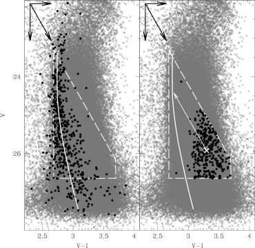
Figure 3.2: $(V,V-I)$ CMD of Terzan 5 zoomed in the MS region (grey crosses). The white dashed lines (same in both panels) delimit the selection box for the stars used for the computation of the differential reddening correction in each cell. The reddening vector is shown in the upper left corners of the diagrams. Left panel– The stars in the least extincted (bluest) cell are marked as black dots and their best-fit is shown as a white solid line. Right panel– The mean color and magnitude of the stars selected in the $i$-th cell (black dots) define the equivalent cell-point ($\langle V-I\rangle$, $\langle V\rangle$), marked as a white cross. The color excess of the cell is obtained by quantifying the shift needed to project this point onto the reference line along the reddening vector.

The accurate inspection of the MS population in each cell allowed us to identify the one with the lowest extinction (i.e. where the MS population shows the bluest average color): it is located in the South-East region of the cluster at a distance $r\simeq 80\mbox{${}^{\prime\prime}$}$ from its center. The stars in this cell are shown in the left panel of Figure 3.2 and those enclosed in the selection box have been used as reference sequence for evaluating the differential reddening in each cell. As a "guide line" of this sequence we used an isochrone of 12 Gyr and metallicity $Z=0.01$ (from Marigo et al., 2008; Girardi et al., 2010) suitably shifted to best-fit the MS star distribution (see the heavy white line in Figure 3.2).

For each cell of the grid we determined the mean $\langle V-I\rangle$ color and $\langle V\rangle$ magnitude. A sigma-clipping rejection at 2-$\sigma$ has been adopted to minimize the contribution of Galactic disc stars (typically much bluer than those of Terzan 5) and any other interloper. Each cell is then described by the ($\langle V-I\rangle,\langle V\rangle$) color-magnitude pair, which defines the equivalent cell-point in the CMD (as an example, see the cross marked in the right panel of Figure 3.2). The relative color excess of each $i$-th cell, $\delta[E(V-I)]_{i}$, is estimated by quantifying the shift needed to move the equivalent cell-point onto the reference sequence along the reddening vector (see the right panel of Figure 3.2). From the value of $\delta[E(V-I)]_{i}$, the corresponding $\delta[E(B-V)]_{i}$ is easily computed using the relation

$$\delta[E(B-V)]_{i}=\frac{\delta[E(V-I)]_{i}}{(R_{V}-R_{I})},$$ (3.1)

where $i=1,m\times n$ and $m\times n=625$ is the total number of cells in our grid. The $V$ and $I$ magnitudes of all stars in the $i$-th cell are then corrected by using the derived $\delta[E(B-V)]_{i}$ and a new CMD is built. The whole procedure is iteratively repeated and a residual $\delta[E(B-V)]_{i}$ is calculated after each iteration. The process stops when the difference in the color excess between two subsequent steps becomes negligible ($\lesssim 0.02$ mag). The final value of the relative color excess in each cell $\delta[E(B-V)]_{i}$ is thus given by the sum over all the iterative steps. For robustness, we applied this procedure in both the $(I,V-I)$ and $(V,V-I)$ planes. The difference between the two estimates turned out to be always smaller than $\sim 0.01$ mag and the average of the two measures was then adopted as the final estimate of the differential reddening in each cell.

3.1.3 Error estimate and caveats

Our estimate of the error associated to the color-excess in each cell is based on the method described by von Braun & Mateo, 2001 (see also Alonso-García et al., 2011). We considered the uncertainty on the mean color of the $i$-th cell as the main source of error on the value of $\delta[E(B-V)]_{i}$. This latter was then computed as the ratio between the 1-$\sigma$ dispersion of the mean color and the parameter $a=\cos(180-\theta)$, where $\theta$ is the angle between the reddening vector and the color-axis. Geometrically, this is equivalent to measure the difference between the values of $\delta[E(B-V)]_{i}$ of the first and last contact-points of the color error-bar when moved along the reddening vector to match the reference line. We did not consider the error on the mean magnitude because, since the reference line is almost vertical, its contribution is negligible. Following these prescriptions we obtain a typical formal error of about $0.03$ mag on each color excess value $\delta[E(B-V)]_{i}$.

A potential problem with this procedure to quantify the differential reddening of Terzan 5 is the presence of two stellar populations with distinct iron abundances. Indeed, the metal-rich population is expected to be systematically redder than the metal-poor one in the CMD, and we therefore expect that at least a fraction of stars with redder colors along the MS are genuine metal-rich objects, and not metal-poor stars affected by a larger extinction. However, by using the Girardi et al. (2010) isochrones, the expected intrinsic difference in the $(V-I)$ color between the metal-rich and metal-poor populations is only $\delta(V-I)\sim 0.05$ mag. Moreover, the metal-rich population has been found to be more centrally segregated than the metal-poor one (F09, L10). Hence, we expect the former to become progressively negligible with increasing radial distance from the cluster center. On the other hand, the uncertainties due to the photometric errors are dominant in the central region of the system, where the two populations are comparable in number. Finally, the use of average values for the color and magnitude in each cell ($\langle V-I\rangle$ and $\langle V\rangle$), with the addition of a sigma-clipping rejection algorithm, should reduce the effect of contamination by metal-rich stars. Thus, an overall error of $0.05$ mag on the color excesses $\delta[E(B-V)]_{i}$ is conservatively adopted to take into account any possible residual effects due to the presence of a double population in Terzan 5.

3.2 Results

The final differential reddening map in the direction of Terzan 5 is shown in Figure 3.3, with lighter colors indicating less obscured regions and the center of gravity and core radius (r_c, see L10) also marked for reference. We find that, within the area covered by the WFC/ACS, the color excess variations can be as large as $\delta E(B-V)=0.67$ mag. This is consistent with the value of 0.69 mag estimated by Ortolani et al. (1996) from the elongation of the RC. The obscuring clouds appear to be structured in two main dusty patches: the first one is located in the North-Western corner of the map at $30\mbox{${}^{\prime\prime}$}-35\mbox{${}^{\prime\prime}$}$ from the center, with an average differential extinction $\delta E(B-V)>0.4$ mag and a peak value of 0.67 mag. The second one is placed in the South-Eastern corner, with typical values of $\delta E(B-V)\sim 0.3$ mag. These two regions seem to be connected by a bridge-like structure with $\delta E(B-V)\gtrsim 0.2-0.3$ mag.

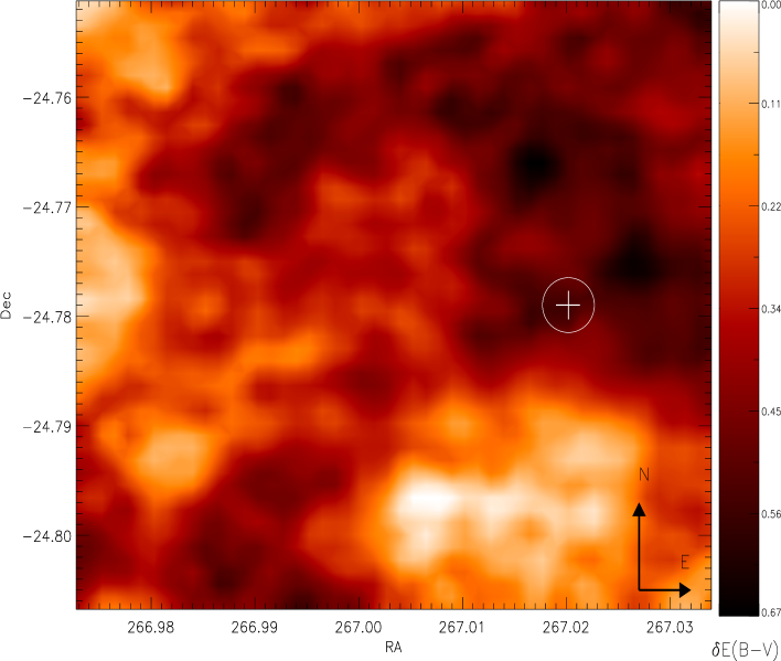
Figure 3.3: Reddening map of the WFC/ACS FoV ($200\mbox{${}^{\prime\prime}$}\times 200\mbox{${}^{\prime\prime}$}$) in the direction of Terzan 5. The differential color excess $\delta E(B-V)$ ranges between zero (lightest) and 0.67 (darkest). The gravity center and core radius of Terzan 5 (L10) are marked for reference as white cross and circle, respectively.

We used this map to correct our photometric catalogue. Figure 3.4 shows the comparison between the observed (left panel) and the differential-reddening corrected (right panel) CMDs in the $(V,V-I)$ plane. After the correction, both the color extension of the RC and the RGB width are significantly reduced by 40% and $>50$%, respectively, and V magnitudes become $\sim 0.5$ mag brighter. To properly quantify the effect of such a correction on the MS width, we selected the stars along an almost vertical portion of MS and compared their color distributions before and after the correction. To this end, we selected stars with $25<V<25.5$ in the observed CMD, and 0.5 mag brighter in the corrected one (see the dashed lines in Figure 3.4). The result is shown in the bottom panels of the figure. Before the correction the MS color distribution is well represented by a Gaussian with a dispersion $\sigma=0.18$, significantly larger than the photometric error at this magnitude level ($\sigma_{phot}\sim 0.13$). Instead, the intrinsic width of the corrected MS is well reproduced by the convolution of two Gaussian functions separated by 0.05 mag in color, with a ratio of 1.6 between their amplitudes, and each one having $\sigma=0.13$ equal to the photometric error. Such a color separation corresponds to what expected for two stellar populations with metallicities equal to those measured in Terzan 5 (see Sect. 3.1.3). The adopted ratio between the amplitudes corresponds to the number counts ratio between metal-poor and metal-rich populations (L10). Hence, these two Gaussian functions correspond to the two sub-populations at different metallicities observed in Terzan 5. Note that the corrected MS color distribution shows an asymmetry toward the redder side, which is more pronounced in the center of the system and decreases at progressively larger distances. The highest amplitude Gaussian (corresponding to the metal-poor population) is unable to properly account for this feature, while the convolution with the reddest and lowest amplitude Gaussian (corresponding to the metal-rich population, which is observed to decrease in number with increasing distance from the center) provides an excellent match.

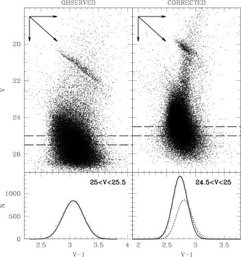
Figure 3.4: Comparison between the optical CMDs of Terzan 5 before (left panel) and after (right panel) the differential reddening correction. Only stars located at a distance $20\mbox{${}^{\prime\prime}$}<r<80\mbox{${}^{\prime\prime}$}$ are plotted for sake of clarity. All the sequences in the corrected CMD are much less stretched along the reddening vector. The bottom panels show the color distributions (grey histograms) for a nearly vertical portion of MS at $25<V<25.5$ in the observed CMD, and at $24.5<V<25$ in the corrected one (see the dashed lines in the two upper panels). Before the correction, the color distribution is well represented by a Gaussian with $\sigma=0.18$ (while the photometric error is $\sigma_{phot}\sim 0.13$). After the correction, the distribution is well fitted by the convolution of two Gaussian functions with $\sigma=0.13$, separated by 0.05 mag in color and with an amplitude ratio of 1.6. The solid Gaussian corresponds to the metal-poor population of Terzan 5, while the dotted one represents the metal-rich component (Sect. 3.2).

The derived reddening correction was also applied to the $(K,V-K)$ CMD obtained from the combination of the ACS and near-infrared data (see F09). Figure 3.5 shows the corrected CMD with two well separated RGB sub-populations and the two distinct RCs. The ratio between the number of stars counted along the two RGBs is $\sim 1.5$, in very good agreement with the value from the RCs (see above and L10).

Figure 3.5: Brightest portion of the differential reddening corrected $(K,V-K)$ CMD of Terzan 5, with error bars also reported. Beside the two RCs, also two well separated RGBs are clearly distinguishable. The solid and dashed lines correspond to the mean ridge lines of the metal-poor and the metal-rich sub-populations, respectively.

The differential reddening corrected CMD can be finally used to estimate the absolute color excess in the direction of Terzan 5. Different values of $E(B-V)$ are provided in the literature, ranging from 1.65 (estimated by Armandroff & Zinn 1988 from the strength of an interstellar band at 8621Å), up to 2.19 and 2.39, derived from optical or infrared photometry (Barbuy et al., 1998; Cohn et al., 2002; Valenti et al., 2007). However, all these estimates are average values and do not take into account the presence of differential reddening. Here, instead, we want to build a 2-dimensional map of the absolute reddening and, to this end, we shifted the corrected $(V,V-I)$ CMD of Terzan 5 along the reddening direction until it matches the CMD of 47 Tucanae, adopted as reference cluster since it is metal-rich, low extincted and with a well-determined distance modulus. In particular we looked for the best match between the RC of the metal-poor population of Terzan 5 and the RC of 47 Tucanae. We adopted the color excess $E(B-V)=0.04$ and the distance modulus $\mu_{0}=13.32$ for 47 Tucanae (from Ferraro et al., 1999), and $\mu_{0}=13.87$ for Terzan 5 (Valenti et al., 2007). From Girardi et al. (2010) model, in the $(V,V-I)$ plane the RC of 47 Tucanae turns out to be 0.02 mag brighter and 0.03 mag bluer than the metal-poor one of Terzan 5 because of a difference in their metallicity ([Fe/H]$=-0.70$ for 47 Tucanae and [Fe/H]$=-0.27$ for the metal-poor population of Terzan 5; see Ferraro et al. 1999 and O11, respectively). Taking into account these slight differences, a nice match of the two RCs is obtained by adopting $E(B-V)=2.15$ mag. Since the corrected CMD is, by construction, referred to the bluest cell, the absolute color excess within the WFC/ACS FoV varies from $E(B-V)=2.15$ up to $E(B-V)=2.82$ mag. In order to check the reliability of these estimates, we compared it with the values found by Gonzalez et al. (2012) from the Vista Variable in the Via Lactea survey. In a $2\mbox{${}^{\prime}$}\times 2\mbox{${}^{\prime}$}$ region centered on Terzan 5, these authors found an extinction $A_{K}=0.80$ mag. Using Cardelli et al. (1989) coefficients to convert $E(B-V)$ to $A_{K}$, our estimate varies from $A_{K}=0.75$ to $A_{K}=0.98$ mag, in nice agreement with Gonzalez et al. (2012) result.

Moreover, we looked for a possible correlation between the color excess and the dispersion measures for 34 MSPs of Terzan 5 studied by Ransom (2007). In this case we did not find a strong correlation, probably because mostly (75%) of the MSP sample is situated within the inner $20\mbox{${}^{\prime\prime}$}$ of the system, where the estimate of $E(B-V)$ is more uncertain (see Sect. 3.1.3).

Chapter 4 Chemical and kinematical properties of Galactic bulge stars surrounding the stellar system Terzan 5

In order to investigate the kinematical and chemical properties of Terzan 5, we have collected spectra for more than 1600 stars in its direction. In this Chapter we focus on the properties of the bulge field population surrounding the system, with the aim of providing crucial information for further studies of both Terzan 5 and the bulge itself. In fact, this is a statistically significant sample of field stars which can be used to decontaminate the population of Terzan 5 from non-members. Moreover, it is one of the few large samples of bulge stars spectroscopically investigated at low and positive latitudes (b$=+1.7$°), thus allowing interesting comparisons with other well studied bulge regions.

The complete description of this analysis can be found in Massari et al. (2014a).

4.1 The sample

This study is based on a sample of 1608 stars within a radius of 800^′′from the center of Terzan 5 ($\alpha_{{\rm J}2000}=17^{\rm h}:48^{\rm m}:4^{\rm s\!.}85$, $\delta_{{\rm J}2000}=-24^{\circ}:46\mbox{${}^{\prime}$}:44\mbox{${}^{\prime\prime}$}6$; see F09, L10). While the overall survey will be described in a forthcoming paper (Francesco Ferraro et al. in preparation), in this work we focus on a sub-sample of stars representative of the field population surrounding Terzan 5. Given the value of the tidal radius of the system (r${}_{t}\simeq 300\mbox{${}^{\prime\prime}$}$; L10, Miocchi et al. 2013), we conservatively selected as genuine field population members all the targets more distant than $400\mbox{${}^{\prime\prime}$}$ from the center of Terzan 5. This sub-sample is composed of $615$ stars belonging to two different datasets obtained with FLAMES (Pasquini et al., 2002) at the ESO-VLT and with DEIMOS (Faber et al. 2003) at the Keck II Telescope. Each target has been selected from the ESO-WFI optical catalog described in L10, along the brightest portion of the RGB, with magnitudes brighter than $I<18.5$. In order to avoid contamination from other sources, in the selection process of the spectroscopic targets we avoided stars with bright neighbors (I${}_{neighbor}<{\rm I_{star}}+1.0$) within a distance of 2^′′. The spatial distribution of the entire sample is shown in Figure 4.1, where the selected field members are shown as large filled circles.

Figure 4.1: Spatial distribution of all the targets in our spectroscopic survey in the direction of Terzan 5. The center of gravity and tidal radius ($r_{t}\simeq 300\mbox{${}^{\prime\prime}$}$) of Terzan 5 (from L10) are marked with a gray cross and a gray dashed circle, respectively. The targets discussed in this work (shown as filled black circles) are all located at more than 400^′′ from the center (gray solid circle), well beyond the Terzan 5 tidal radius.

The FLAMES dataset was collected under three different programs: 087.D-0716(B), PI: Ferraro; 087.D-0748(A), PI: Lovisi; and 283.D-5027(A), PI: Ferraro. All the spectra were acquired in the GIRAFFE/MEDUSA mode, allowing the allocation of 132 fibers across a $25\mbox{${}^{\prime}$}$ diameter FoV in a single pointing. We used the GIRAFFE setup HR21, with a resolving power of 16200 and a spectral coverage ranging from 8484 Å to 9001 Å. This grating was chosen because it includes the prominent Ca II triplet lines, which are excellent features to measure radial velocities also in relatively low signal-to-noise ratio (SNR) spectra. Other metal lines (mainly Fe I) lie in this spectral range, thus allowing a direct measurement of the iron abundance. Multiple exposures (with integration times ranging from 1500 to 3000 s, according to the magnitude of the targets) were secured for the majority of the stars, in order to reach SNR$\sim$30 even for the faintest ($I\sim 18.5$) targets. The data reduction was performed with the FLAMES-GIRAFFE pipeline, including bias-subtraction, flat-field correction, wavelength calibration with a standard Th-Ar lamp, re-sampling at a constant pixel-size and extraction of one-dimensional spectra. Since a correct sky subtraction is particularly crucial in this spectral range (because of the large number of O₂ and OH emission lines), 15-20 fibers were used to measure the sky in each exposure. Then a master sky spectrum was obtained from the median of these spectra and it was subtracted from the target spectra. Finally, all the spectra were shifted to zero-velocity and in the case of multiple exposures they were co-added.

The DEIMOS dataset was acquired using the 1200 line/mm grating coupled with the GG495 and GG550 order-blocking filters, covering the $\sim$6500-9500 Å spectral range at a resolution of R$\sim$7000 at $\sim$8500 Å. The DEIMOS FoV is $16$^′$\times 5$^′, allowing the allocation of more than 100 slits in a single mask. The observations were performed with an exposure time of 600 s, securing SNR$\sim$50-60 spectra for the brightest targets and achieving SNR$\sim$15-20 for the faintest ones (I$\sim 17$). The spectra have been reduced by means of the package developed for an optimal reduction and extraction of DEIMOS spectra and described in Ibata et al. (2011).

4.2 Radial velocities

Radial velocities ($v_{\rm rad}$) for the target stars were measured by cross-correlating the observed spectra with a template of known velocity, following the procedure described in Tonry & Davis (1979) and implemented in the FXCOR software under IRAF. As templates we adopted synthetic spectra computed with the SYNTHE code (Sbordone et al., 2004). For most of the stars the cross-correlation procedure is performed in the spectral region $\sim$8490-8700 Å, including the prominent Ca II triplet lines that can be well detected also in noisy spectra. For some very cool stars, strong TiO molecular bands dominate this spectral region, preventing any reliable measurement of the Ca features (Figure 4.2 shows the comparison between two FLAMES spectra, with and without strong molecular bands). In these cases, the radial velocity was measured from the TiO lines by considering only the spectral region around the TiO bandhead at $\sim$8860 Å and by using as template a synthetic spectrum including all these features. Because several stars show both the Ca II triplet lines and weak TiO bandheads, for some of them the radial velocity has been measured independently using the two spectral regions. We always found an excellent agreement between the two measurements, thus ruling out possible offsets between the two $v_{\rm rad}$ diagnostics.

Figure 4.2: Examples of spectra poorly (solid line) and severely (dashed line) affected by the TiO molecular bands ($\lambda>8860$ Å). The gray regions highlight the wavelength ranges adopted to compute the $q$-parameter defined in the text (Section 4.3). For these two spectra very different values of $q$ have been obtained: $q=0.94$ and $q=0.28$ for the solid and dashed spectrum, respectively. According to the adopted selection criterion (q$>0.6$), the iron abundance has not been computed from the latter.

For the FLAMES dataset, where multiple exposures were secured for most of the stars, radial velocities were obtained from each exposure independently. The final radial velocity is computed as the weighted mean of the individual velocities (each corrected for its own heliocentric velocity), by using the formal errors provided by FXCOR as weights. For the DEIMOS spectra, we checked for possible velocity offsets due to the mis-centering of the target within the slit (see the discussion about this effect in Simon & Geha, 2007), through the cross-correlation of the A telluric band (7600-7630 Å). We found these offsets to be of the order of few km s^-1. The uncertainty on the determination of this correction (always smaller than 1 km s^-1) has been added in quadrature to that provided by FXCOR. The typical final error on our measured v_rad is $\sim 1.0$ km s^-1.

The distribution of the measured $v_{\rm rad}$ for the 615 targets is shown in Figure 4.3. It ranges from $-264.0$ km s^-1 to $+303.9$ km s^-1. By using a Maximum-Likelihood procedure, we find that the Gaussian function that best describes the distribution has mean $\langle v_{\rm rad}\rangle=21.0\pm 4.6$ km s^-1 and $\sigma_{v}=113.0\pm 2.7$ km s^-1. We converted radial velocities to Galactocentric velocities ($v_{\rm GC}$) by correcting for the Solar reflex motion (220 km s^-1; Kerr & Lynden-Bell 1986) and assuming as peculiar velocity of the Sun in the direction (l,b)$=$(53°,25°) $v=18.0$ km s^-1 (Schönrich et al., 2010). The conversion equation is then:

$$v_{{\rm GC}}=v_{{\rm rad}}+220[\sin(l)\cos(b)]+18[\sin(b)\sin(25)+\cos(l)\cos(25)\cos(l-53)],$$ (4.1)

where velocities are in km s^-1, and (l,b)=(3.8°, 1.7°) is the location of Terzan 5. The Galactocentric velocity distribution estimated in this way peaks at $<v_{{\rm GC}}>=47.7\pm 4.6$ km s^-1.

Figure 4.3: Radial velocity distribution for the 615 spectroscopic targets at $r>400\mbox{${}^{\prime\prime}$}$. The mean value and dispersion are indicated. The bin size (20 km s^-1) is the same as that adopted by Nidever et al. (2012), but in our case no high velocity sub-components are found. The systemic velocity of Terzan 5 (v${}_{{\rm rad}}\simeq-83$ km s^-1) and the location of the subcomponent found in Nidever et al. (2012) (v${}_{{\rm rad}}\simeq 200$ km s^-1) are also marked with the black arrows for sake of comparison.

This value turns out to be in good agreement with the values found in the context of three recent kinematic surveys of the Galactic bulge: the BRAVA survey (Rich et al. 2007), the ARGOS survey (Freeman et al. 2013) and the GIBS survey (Zoccali et al. 2014). In fact, in fields located close to the Galactic Plane and with Galactic longitude as similar as possible to ours, Howard et al. (2008, see also Kunder et al. 2012) found $<v_{{\rm GC}}>=53.0\pm 10.3$ km s^-1 at (l,b)=(4°,-3.5°) for BRAVA, Ness et al. (2013b) found $<v_{{\rm GC}}>=44.4\pm 3.8$ km s^-1 at (l,b)=(5°,-5°) for ARGOS and Zoccali et al. (2014) obtained $<v_{{\rm GC}}>=55.9\pm 3.9$ km s^-1 at (l,b)=(3°,-2°) for GIBS. Thus, all the measurements agree within the errors with our result. As for the velocity dispersion, our estimate ($\sigma_{v}=113\pm 2.7$ km s^-1) agrees well with the result of Kunder et al. (2012), who found $\sigma_{v}=106$ km s^-1, and with that of Zoccali et al. (2008) who measured $\sigma_{v}=112.5\pm 6.4$ km s^-1. Instead, it is larger than that quoted in Ness et al. (2013b) $\sigma_{v}=92.2\pm 2.7$ km s^-1. Since their field is the farthest from ours among those selected for the comparison, we ascribe such a difference to the different location in the bulge. As a further check, we used the Besançon Galactic model (Robin et al. 2003) to simulate a field with the same size of our photometric sample (i.e., the WFI FoV) around the location of Terzan 5, and we selected all the bulge stars lying within the same color and magnitude limits of our sample. The velocity dispersion for these simulated stars is $\sigma_{v}=119$ km s^-1, in agreement with our estimate.

It is worth mentioning that Nidever et al. (2012) identified a high velocity ($v_{{\rm rad}}\sim$200 km s^-1) sub-component that accounts for about 10% of their entire sample of $\sim 4700$ bulge stars. Such a feature has been found in eight fields located at -4.3°$<$b$<2$°and 4°$<$l$<14$°. Nidever et al. (2012) suggest that such a high-velocity feature may correspond to stars in the Galactic bar which have been missed by other surveys because of the low latitude of the sampled fields. However, as is evident in Figure 4.3 (where we adopted the same bin-size used in Fig. 2 of Nidever et al. (2012) for sake of comparison), we do not find neither high-velocity peak nor isolated substructures in our sample, despite its low latitude. In fact, the skewness calculated for our distribution is $-0.02$, clearly demonstrating its symmetry. Also Zoccali et al. (2014) did not find any significant peak at such large velocity in the recent GIBS survey.

4.3 Metallicities

For a sub-sample of $284$ stars we were able to also derive metallicity. As already pointed out in Section 4.2, spectra of cool giants are affected by the presence of prominent TiO molecular bands. These bands make particularly uncertain the determination of the continuum level. While this effect has no consequences on the determination of radial velocities, it could critically affects the metallicity estimate. Therefore we limited the metallicity analysis only to stars whose spectra suffer from little contamination from the TiO bands. In order to properly evaluate the impact of the TiO bands in the considered wavelength range, we performed a detailed analysis of a large set of synthetic spectra and we defined a parameter $q$ as the ratio between the flux of the deepest feature of the TiO bandhead at 8860 Å (computed as the minimum value in the spectral range 8859.5 Å$<\lambda<$8861 Å) and the continuum level measured with an iterative 3 $\sigma$-clipping procedure in the adjacent spectral range, 8850Å$<\lambda<$8856 Å (see the shaded regions of Figure 4.2).

We found that the continuum level of synthetic spectra for stars with $q>0.8$ is slightly ($<2\%$) affected by TiO bands over the entire spectral range, while for stars with $0.6<q<0.8$ the region marginally ($<5\%$) affected by the contamination is confined between 8680 Å and 8850 Å. Instead, stars with $q<0.6$ have no useful spectral ranges (where at least one of the Fe I in our linelist falls) with TiO contamination weak enough to allow a reliable chemical analysis. We therefore analyzed targets with $q>0.8$ (counting 126 objects) using the full linelist (see Section 4.3.2), while for targets with $0.6<q<0.8$ (158 objects) only a sub-set of atomic lines lying in the safe spectral range $8680-8850$ Å has been adopted. All targets with $q<0.6$ (329 stars) have been excluded from the metallicity analysis. Hence the metallicity analysis is limited to 284 stars (corresponding to $\sim 46\%$ of the entire sample observed in the spectroscopic survey). In Section 4.3.5 we discuss the impact of this selection on the results of the analysis.

4.3.1 Atmospheric parameters

We derived effective temperatures (T_eff) and gravities ($\log$ $g$) photometrically. In order to minimize the effect of differential reddening we used the 2MASS catalog, correcting the (K, J-K) CMD for differential extinction according to our new wide-field reddening map, shown in Figure 4.4. This was obtained by applying to the optical WFI catalog the same procedure described in Chapter 3. Because of the large incompleteness at the MS level we were forced to use red clump stars as reference. Since these stars are significantly less numerous than MS stars, the spatial resolution of the computed reddening map ($60\mbox{${}^{\prime\prime}$}\times 60\mbox{${}^{\prime\prime}$}$) is coarser than that ($8\mbox{${}^{\prime\prime}$}\times 8\mbox{${}^{\prime\prime}$}$) published in Massari et al. (2012) for the HST ACS field of view. However, despite this difference in resolution, the WFI reddening map agrees quite well with that for ACS in the overlapping region. Indeed for the stars in common between the two catalogs, the average difference between the differential reddening estimates is $\langle\Delta E(B-V)\rangle=0.01$ mag with a dispersion $\sigma=0.1$ mag. This latter value is also the uncertainty that we conservatively adopt for our color excess estimates.

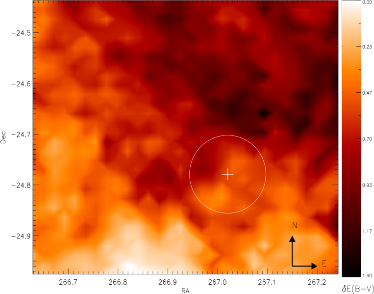
Figure 4.4: Reddening map in the direction of Terzan 5 covering the entire $\sim 25$^′$\times 25$^′ FoV. Dark colors correspond to regions of large extinction (see the color bar on the right). The center and tidal radius of Terzan 5 are marked for sake of comparison.

Figure 4.5 shows the IR CMD after the internal reddening correction, with the positions of the spectroscopic targets highlighted. To determine T_eff, we adopted the (J-K)${}_{0}-$T_eff empirical relation quoted by Montegriffo et al. (1998). Since the relation is calibrated onto the SAAO photometric system, we previously converted our 2MASS magnitudes following the prescriptions in Carpenter (2001). To estimate photometric gravities, we used the relation:

$$\log g=\log g_{\odot}+4\log(T_{{\rm eff}}/T_{\odot})+\log(M/M_{\odot})+0.4(M_{{\rm bol}}-M_{{\rm bol},\odot})$$ (4.2)

adopting $\log$ $g_{\odot}$=4.44 dex, T_⊙=$5770$ K, M${}_{{\rm bol},\odot}=4.75$, M$=0.8$ M_⊙ and a distance of 8 kpc. Such a distance is the average value predicted by the Besançon model for a simulated field with the size of the FoV covered by our observations and centered around Terzan 5. This value is also normally adopted when bulge stars are analyzed (Zoccali et al. 2008; Alves-Brito et al. 2010; Hill et al. 2011, see also Sect. 4.3.5 for a discussion on the impact of distance on our results). Bolometric corrections were taken from Montegriffo et al. (1998). The small number (about 10) of Fe I lines available in the spectra prevents us to derive reliable values of microturbulent velocity ($v_{turb}$; see Mucciarelli 2011 for a review of the different methods to infer this parameter). We therefore referred to the works of Zoccali et al. (2008) and Johnson et al. (2013) on large samples of bulge giant stars characterized by metallicities and atmospheric parameters similar to those of our targets. Since no specific trend between $v_{turb}$ and the atmospheric parameters is found in these samples, we adopted their median velocity $v_{turb}=$1.5 km s^-1 ($\sigma=0.16$ km s^-1) for all the targets.

Figure 4.5: (K, J-K) CMD corrected for internal differential extinction, for all the stars located at $400\mbox{${}^{\prime\prime}$}<r<800\mbox{${}^{\prime\prime}$}$ from the center of Terzan 5, in our ESO-WFI photometric sample (small dots). The spectroscopic targets are shown with large symbols. The targets for which iron abundance could be estimated are highlighted as large filled circles. The three strips adopted to evaluate the impact of the selection bias discussed in the text (Section 4.3.5) are shown. The horizontal dashed lines delimit the bias-free sample adopted to derive the metallicity distribution shown as a grey histogram in Figure 4.6.

4.3.2 Chemical analysis

The Fe I lines used for the chemical analysis were selected from the latest version of the Kurucz/Castelli dataset of atomic data. We included only Fe I transitions found to be unblended in synthetic spectra calculated with the typical atmospheric parameters of our targets and at the resolutions provided by the GIRAFFE and DEIMOS spectrographs. These synthetic spectra were calculated with the SYNTHE code, including the entire Kurucz/Castelli line-list (both for atomic and molecular lines) convolved with a Gaussian profile at the resolution of the observed spectra. Due to the different spectral resolution of the two datasets, we used two different techniques to analyze the spectral lines and determine the chemical abundances.

(1) FLAMES spectra— The chemical analysis was performed using the package GALA (Mucciarelli et al., 2013), an automatic tool to derive the chemical abundances of single, unblended lines by using their measured equivalent widths (EWs). The adopted model atmospheres were calculated with the ATLAS9 code (Castelli & Kurucz, 2004). In our analysis, we run GALA fixing all the atmospheric parameters estimated as described above and leaving only the metallicity of the model atmosphere free to vary iteratively in order to match the iron abundance derived from EWs. EWs were obtained with the code 4DAO (Mucciarelli 2013), aimed at running DAOSPEC (Stetson & Pancino, 2008) for a large set of spectra, tuning automatically the main input parameters used by DAOSPEC and providing graphical outputs to visually inspect the quality of the fit for each individual spectral line. The EWs were measured adopting a Gaussian function that is a reliable approximation for the line profile at the resolution of our spectra. EW errors were estimated by DAOSPEC from the standard deviation of the local flux residuals (see Stetson & Pancino, 2008) and lines with EW errors larger than 10% were rejected.

(2) DEIMOS spectra— Due to the low resolution of the DEIMOS spectra, the high degree of line blending and blanketing makes the derivation of the abundances through the method of the EWs quite complex and uncertain. Thus, the iron abundances were measured by comparing the observed spectra with a grid of synthetic spectra, following the procedure described in Mucciarelli et al. (2012). Each Fe I line was analyzed independently by performing a $\chi^{2}$-minimization between the normalized observed spectrum and a grid of synthetic spectra (computed with the code SYNTHE, convolved at DEIMOS resolution and resampled at the pixel-size of the observed spectra). Then, the normalization is readjusted locally in a region of $\sim$50-60 Å in order to improve the quality of the fit. Uncertainties in the fitting procedure for each spectral line were estimated by using Monte Carlo simulations: for each line, Poissonian noise was added to the best-fit synthetic spectrum in order to match the observed SNR, and then the fit was re-computed with the same procedure described above. A total of 1000 Monte Carlo realizations has computed for each line, and the dispersion of the derived abundance distribution was adopted as the abundance uncertainty. Typical values are of about $\pm$0.2 dex.

4.3.3 Calibration stars

Because of its prominence, the Ca II triplet is commonly used as a proxy of the metallicity. However, several Fe I lines fall in the spectral range of the adopted FLAMES and DEIMOS setups and we therefore decided to measure the iron abundance directly from these lines. To demonstrate the full reliability of the atomic data adopted to derive the metallicity we performed the same analysis on a set of high-resolution, high-SNR spectra of the Sun and of Arcturus. For the Sun we adopted the solar flux spectrum quoted by Neckel & Labs (1984), while for Arcturus we used the high-resolution spectrum of Hinkle et al. (2000). Both spectra were analyzed by adopting the same linelist used for the targets of this study. For the Sun, the solar model atmosphere computed by F. Castelli was used (T_eff=5777 K, $\log$ $g$=4.44 dex), and v_turb=1.2 km s^-1 (Andersen et al. 1999) was adopted. For Arcturus we calculated a suitable ATLAS9 model atmosphere with the atmospheric parameters (T_eff=5286 K, $\log$ $g$=1.66 dex, v_turb=1.7 km s^-1) listed by Ramirez & Allende Prieto (2011). The resulting iron abundance for the Sun is A(Fe I)_Sun=7.49$\pm$0.03 dex, in very good agreement with that listed by Grevesse & Sauval (1998, A(Fe)$=7.50$). For Arcturus we obtained A(Fe I)_Arcturus=7.00$\pm$0.02, corresponding to [Fe/H]$=-0.50\pm 0.02$ dex, in excellent agreement with the measure of Ramirez & Allende Prieto (2011) who quote [Fe/H]$=-0.52\pm 0.02$. Thus, we conclude that the adopted atomic lines provide a reliable estimate of the iron abundance.

As discussed in Section 4.3, for the 158 stars with $0.6<q<0.8$ we limited the metallicity analysis to the iron lines in a restricted wavelength range ($8680-8850$ Å) poorly affected by the TiO bands. In order to properly check for any possible systematic effect due to the different line list adopted, we re-performed the metallicity analysis of the 126 stars with $q>0.8$ using only the reduced line list. We found a very small off-set in the derived abundance ($\delta[Fe/H]=$[Fe/H]_full-[Fe/H]${}_{reduced}=-0.06\pm 0.01$ dex), that was finally applied to the iron abundance obtained for the 158 low-$q$ targets.

4.3.4 Uncertainties

The global uncertainty of our iron abundance estimates (typically $\sim 0.2$ dex) is computed as the sum in quadrature of two different sources of error. The first one is the error arising from the uncertainties on the atmospheric parameters. Since they have been derived from photometry, the formal uncertainty on these quantities depends on all those parameters which can affect the location of the targets in the CMD, such as photometric errors, uncertainty on the absolute and differential reddening and errors on the distance modulus (DM). In order to evaluate the uncertainties on $T_{eff}$ and $\log$ $g$ we therefore repeated their estimates for every single target assuming $\sigma_{K}=0.04$, $\sigma_{J-K}=0.05$, $\sigma_{\delta[E(B-V)]}=0.1$ (see Section 4.3.1), $\sigma_{[E(B-V)]}=0.05$ (Massari et al. 2012) and a conservative value $\sigma_{\rm DM}=0.3$ (corresponding to $\pm 1$ kpc) for the DM. Following this procedure we found uncertainties of $\pm 160$ K in T_eff and $\pm 0.2$ dex in $\log$ $g$. For $v_{turb}$ we adopted a conservative uncertainty of 0.2 km s^-1 (see Section 4.3.1). To estimate the impact of these uncertainties on the iron abundance, we repeated the chemical analysis assuming, each time, a variation by 1$\sigma$ of any given parameter (keeping the other ones fixed).

The second source of error comes from the internal abundance estimate uncertainty. For each target this was estimated as the dispersion around the mean of the abundances derived from the used lines, divided by the root square of the number of lines. It is worth noticing that for any given star the dispersion is calculated by weighting the abundance of each line by its own uncertainty (as estimated by DAOSPEC for the FLAMES targets, and from Monte Carlo simulations for the DEIMOS targets).

4.3.5 Results

The iron abundances and their total uncertainties for each of the 284 targets analyzed are listed in Table 4.1, together with the adopted atmospheric parameters. The [Fe/H] distribution for the entire sample is shown as a dashed-line histogram in Figure 4.6. The distribution is quite broad, extending from [Fe/H]$\simeq-1.2$ dex, up to [Fe/H]$\simeq 0.8$ dex, with a pronounced peak at [Fe/H]$=-0.25$ dex. However, the exclusion of a significant fraction of stars with spectra seriously contaminated by TiO bands (see Setc. 4.3), possibly introduced a selection bias on the derived metallicity distribution. In fact prominent TiO bands are preferentially expected in the coolest and reddest stars. This is indeed confirmed by Figure 4.5, showing that the targets for which no abundance measure was feasible (open circles) preferentially populate the brightest and coolest portion of the RGB. Since this is also the region were the most metal-rich stars are expected to be found, in order to provide a meaningful metallicity distribution, representative of the bulge population around Terzan 5, we restricted our analysis to a sub-sample of targets likely not affected by such a bias. To this purpose, in the CMD corrected for internal reddening we selected only stars in the magnitude range $9.2<K_{c}<9.8$ (see dashed lines in Figure 4.5), where metallicity measurements have been possible for 82% of the surveyed stars (i.e., 112 objects over a total of 136). The metallicity distribution for this sub-sample is shown as a grey histogram in the top panel of Figure 4.6. The distribution is still quite broad, extending from [Fe/H]$\simeq-1.2$ dex up to [Fe/H]$\simeq 0.7$ dex, but the sub-solar component (with $-0.5<$[Fe/H]$<0$ dex) seems to be comparable in size to the super-solar component (with $0<$[Fe/H]$<0.5$ dex).

Figure 4.6: Top panel: Metallicity distribution of the bulge field around Terzan 5 for the entire sample of 284 stars (dashed histogram) and for the sub-set of 112 targets selected at $9.2<K_{c}<9.8$ (grey histogram), free from the bias introduced by the TiO bands (which preferentially affects the spectra of the most metal-rich objects). Bottom panel: Metallicity distribution observed in the unbiased sub-set of stars (the same grey histogram as above), compared to the generalized distribution (solid line) obtained from 1000 realization described in the text (Section 4.3.5). The dashed lines delimit the metallicity ranges adopted to define the R_l/h parameter (see text). The percentage of stars in each metallicity range is also marked.

In order to properly evaluate the existence of any residual bias, we followed the method described in Zoccali et al. (2008). We considered three strips in the CMD roughly parallel to the slope of the bulge RGB (Figure 4.5). In each strip, we computed the fraction $f$ defined as the ratio between the number of stars with measured metallicity and the number of targets observed in the spectroscopic surveys. In the selected sub-sample, the $f$ parameter ranges from 0.75 up to 0.90, with the peak in the central bin and with the reddest bin being the less sampled. In order to evaluate the impact of this residual inhomogeneity on the derived metallicity distribution we randomly subtracted from the bluest and central bins a number of stars (2 and 18, respectively) suitable to make the $f$ ratio constant in all the strips. We repeated such a procedure $1000$ times, and for each iteration a new metallicity distribution has been computed. The bottom panel of Figure 4.6 shows the generalized distribution obtained from the entire procedure, overplotted to the observed one. As can be seen, the two distributions are fully compatible, thus providing the final confirmation that the observed distribution is not affected by any substantial residual bias. Hence it has been adopted as representative of the metallicity distribution of the bulge population around Terzan 5.

Table 4.1: Identification number, coordinates, atmospheric parameters, iron abundances and their uncertainties for the Terzan 5 field stars in our sample.

ID	RA	Dec	Teff	log $g$	[Fe/H]	$\sigma_{[Fe/H]}$	Dataset
			(K)	(dex)	(dex)	(dex)
1030711	267.1829348	-24.6923402	3922	0.6	-0.22	0.22	FLAMES
1052484	267.1470436	-24.6830821	4220	0.8	-0.19	0.19	FLAMES
1071029	267.1182806	-24.6825530	3971	1.9	0.39	0.18	FLAMES
1071950	267.1169145	-24.6630493	3832	0.9	0.24	0.19	FLAMES
1072160	267.1165783	-24.6588856	4111	0.9	0.63	0.20	FLAMES
2009060	267.0686838	-24.6638585	4434	0.9	-0.34	0.17	FLAMES
2029939	267.0366131	-24.6637204	4366	1.4	0.69	0.15	FLAMES
2065353	266.9816844	-24.6414183	4013	0.9	-0.04	0.26	FLAMES
2066891	266.9791962	-24.6560448	4371	1.1	0.22	0.19	FLAMES
2068105	266.9771994	-24.6119254	3888	0.9	0.04	0.22	FLAMES

Note. — The entire table is available in the online version of the journal.

In order to compare our results with previous studies, in Figure 4.7 we show the metallicity distribution obtained in the present work and those derived in different regions of the Galactic bulge: $-6$°$<$b$<-2$°(for a sub-sample of micro-lensed dwarfs Bensby et al., 2013), the Baade’s window (for a sub-sample of giants; Hill et al., 2011 and Zoccali et al., 2008), l$=-5.5$°, b$=-7$°(for a sample of giants; Johnson et al., 2013), and the Ness et al. (2013a) field closest to the Galactic disk, at b$=-5$°. The distributions appear quite different. However a few common characteristics can be noted and deserve a brief discussion. Apart from the presence of more or less pronounced peaks, all the distributions show: ($i$) a major sub-solar ([Fe/H]$\simeq-0.2$ dex) component; ($ii$) a super-solar component ([Fe/H]$\simeq 0.2$ dex); ($iii$) a quite extended tail towards low metallicities (reaching [Fe/H]$\simeq-1.5$ dex). However, the relative percentage in the two prominent components appears to be different from one field to another. In order to properly quantify this feature, we defined the ratio R${}_{l/h}=$N${}_{l}/$N_h, where N_l is the number of stars in the sub-solar component (with $-0.5<$[Fe/H]$<0$ dex) and N_h is the number of stars in the super-solar component (with $0<$[Fe/H]$<0.5$ dex). The value of R_l/h is labelled in each panel of Figure 4.7.

Figure 4.7: Comparison of the iron distribution in a few bulge fields at different Galactocentric locations. The corresponding references and Galactic coordinates are indicated in each panel. Vertical dashed lines delimitate the metallicity ranges defining the sub- and super-solar metallicity components. The value of the R_l/h parameter defined in the text (Section 4.3.5) is also reported in each panel.

In Figure 4.8 we plot the value of R_l/h for 13 bulge regions at different latitudes published in the literature (see e.g. Bensby et al. 2013, Hill et al. 2011, Zoccali et al. 2008, Johnson et al. 2011, 2013, Gonzalez et al. 2011, Ness et al. 2013a). The value obtained for the bulge field around Terzan 5 is shown as a large filled circle. It is interesting to note how the populations observed in the 13 reference fields define a clear trend, suggesting that the super-solar component tends to be dominant at latitudes below $|$b$|<5$°. The field around Terzan 5 is located at the lowest latitude observed so far. It nicely fits into this trend, and it suggests the presence of a plateau at R${}_{l/h}\sim 0.8$ for $|$b$|<4$°(see also Rich, Origlia & Valenti 2012). On the other hand, the Galactic location of the field can possibly be the reason for the small amount of stars detected with [Fe/H]$<-0.5$. Figure 4.9 shows the fraction (f_MP) of metal-poor objects (with [Fe/H]$<-0.5$) with respect to the total number of stars for each of the samples described in Figure 4.8, as a function of $|$b$|$. Also in this case a clear trend is defined: the percentage of metal-poor stars drops from $\sim 40$% at $|$b$|\sim 10$°  to a few percent at the latitude of Terzan 5, the only exception being the most external field of Zoccali et al. (2008). Our findings are in good agreement with several recent results about the general properties of the Galactic bulge. Indeed, metal-rich stars are dominant at low Galactic latitudes, that is closer to the Galactic plane (see e.g. Ness et al., 2014, and references therein). Also, we checked the impact on these findings of the assumption of a $8$ kpc distance. We repeated the chemical analysis by adopting distances of $6$ and $10$ kpc. The change of the surface gravity (on average $+0.25$ dex and $-0.2$ dex, respectively) leads to only small differences in the measured [Fe/H], with the stellar metallicities differing on average by $0.06$ dex ($\sigma=0.04$ dex) and $-0.05$ dex ($\sigma=0.02$ dex), in the two cases. Such a tiny difference moves the value of R_l/h from $0.89$ to $0.58$ and $1.26$, respectively, leaving it fully compatible with a flat behavior for $|$b$|<4$° in both cases, while it does not change significantly (less than 1%) the value of f_MP. We underline that this is the first determination of the spectroscopic metallicity distribution for a significant sample of stars at these low and positive Galactic latitudes. Other spectroscopic surveys at low latitudes are needed to confirm the existence of these features.

Figure 4.8: R_l/h parameter as a function of the Galactic latitude (absolute value). The 13 fields taken from the literature nicely describe a metallicity gradient, suggesting that the super-solar component increases with decreasing Galactic latitude. The field measured around Terzan 5 is highlighted with a large filled circle and possibly suggests the presence of a “plateau” at R${}_{l/h}\simeq 0.8$ for $|$b$|<4$°.

Finally it is worth commenting on the velocity dispersion obtained for the two main metallicity components in the field surrounding Terzan 5. We found two similar values, $\sigma_{v}=108\pm 8$ km s^-1 and $\sigma_{v}=111\pm 11$ km s^-1 for the sub-solar and the super-solar component, respectively. The two measured values are in agreement with those observed in the fields at b$=-5$° and at low longitudes (l$<5$°) by Ness et al. (2013b, see the red diamonds in the lower panels of their Figure 7) in the same metallicity range (-0.5$<$[Fe/H]$<0.5$ dex).

Figure 4.9: Fraction of metal-poor stars with [Fe/H]$<-0.5$ dex (f_MP) as a function of the absolute value of the Galactic latitude. The considered bulge fields are the same as those in Fig. 4.8 and also in this case they describe a clear trend, with the only exception of the survey at the largest latitude (from Zoccali et al. 2008). The field measured around Terzan 5 is highlighted with a large filled circle and fits very well into the correlation.

4.4 Summary

We determined the radial velocity distribution for a sample of 615 stars at (l,b)=(3.7°,1.8°), representative of the bulge field population surrounding the peculiar stellar system Terzan 5. We found that the distribution is well fitted by a Gaussian function with $<v_{\rm rad}>=21.0\pm 4.6$ km s^-1 and $\sigma_{v}=113.0\pm 2.7$ km s^-1. Once converted to Galactocentric velocities, these values are in agreement with the determinations obtained in other bulge fields previously investigated. We did not find evidence for the high-velocity sub-component recently identified in Nidever et al. (2012).

Because of the strong contamination of TiO bands, we were able to measure the iron abundance only for a sample of 284 stars (corresponding to $\sim 46\%$ of the entire sample) and we could derive an unbiased metallicity distribution only from a sub-sample of 112 stars with $9.2<K_{c}<9.8$. Statistical checks have been used to demonstrate that this is a bias-free sample representative of the bulge population around Terzan 5. The metallicity distribution turns out to be quite broad with a peak at [Fe/H]$\simeq+0.05$ dex and it follows the general metallicity-latitude trend found in previous studies, with the number of super-solar bulge stars systematically increasing with respect to the number of sub-solar ones for decreasing latitude. Indeed the population ratio between the sub-solar and super solar components (quantified here by the parameter R_l/h) measured around Terzan 5 nicely agrees with that observed in other low latitude bulge fields, possibly suggesting the presence of a plateau for $|$b$|<4$°. Moreover, also the fraction of stars with [Fe/H]$<-0.5$ measured around Terzan 5 fits well into the correlation with $|$b$|$ found from previous studies.

Chapter 5 The Terzan 5 puzzle: discovery of a third, metal-poor component

In this Chapter we present the discovery of 3 red giant stars belonging to Terzan 5, with metallicity [Fe/H]$\simeq-0.8$ dex, significantly smaller than that of the sub-Solar component previously detected (F09, O11).

For all the details regarding such a discovery see Origlia et al. (2013).

5.1 Observations and chemical abundance analysis

In the context of an ongoing spectroscopic survey with VLT-FLAMES and Keck-DEIMOS of the Terzan 5 stellar populations, aimed at constructing a massive database of radial velocities and metallicities (Massari et al. 2014a; Ferraro et al.; 2014 in preparation), we found some indications of the presence of a minor ($\sim 3\%$) component significantly more metal-poor than the sub-Solar population of Terzan 5. We acquired high resolution spectra of 3 radial velocity candidate metal-poor giants members of Terzan 5. Observations using NIRSPEC (McLean et al., 1998) at Keck II were undertaken on 17 June 2013. We used the NIRSPEC-5 setting to enable observations in the $H$-band and a $0.43\mbox{${}^{\prime\prime}$}$ slit width that provides an overall spectral resolution R=25,000.

Data reduction has been performed by using the REDSPEC IDL-based package developed at the UCLA IR Laboratory. Each spectrum has been sky subtracted by using nod pairs, corrected for flat-field and calibrated in wavelength using arc lamps. An O-star spectrum observed during the same night has been used to remove to check and remove telluric features. The SNR per resolution element of the final spectra is always $>$30. Figure 5.1 shows portions of the observed spectra and the comparison with a Terzan 5 giant with similar stellar parameters and higher iron content from the sub-Solar population studied by O11.

Figure 5.1: Portion of the NIRSPEC $H$-band spectra of two red giants of Terzan 5 with similar temperature ($\rm T_{eff}\approx 3800$ K), but different chemical abundance patterns (solid line for the metal-poor star #243, dotted line for a sub-Solar star at [Fe/H]$\approx$-0.22 from O11). The metal poor giant #243 has significantly shallower features. A few atomic lines and molecular bands of interest are marked.

We compare the observed spectra with synthetic ones and we obtain accurate chemical abundances of C and O using molecular lines and of Fe, Ca, Si, Mg, Ti and Al using neutral atomic lines, as also described in O11 and references therein.

We made use of both spectral synthesis analysis and equivalent width measurements of isolated lines. Synthetic spectra covering a wide range of stellar parameters and elemental abundances have been computed by using the same code as in O11 and described in detail in Origlia, Rich & Castro (2002) and Origlia & Rich (2004). The code uses the LTE approximation, the molecular blanketed model atmospheres of Johnson, Bernat & Krupp (1980) at temperatures $\leq$4000 K, and the Grevesse & Sauval (1998) abundances for the Solar reference.

Stellar temperatures have been first estimated from colors, by using the reddening estimates by Massari et al. (2012) and the color-temperature scale by Montegriffo et al. (1998), calibrated on globular cluster giants. Gravity has been estimated from theoretical isochrones (Pietrinferni et al., 2004, 2006), according to the position of the stars on the RGB. An average microturbulence velocity of 2 km/s has been adopted (see e.g. Origlia et al., 1997, for a detailed discussion). The simultaneous spectral fitting of the CO and OH molecular lines that are especially sensitive to temperature, gravity and microturbulence variations (see also Origlia, Rich & Castro, 2002), allow us to fine-tune our best-fit adopted stellar parameters.

5.2 Results

Our provisional estimate for the systemic velocity of Terzan 5, as inferred from our VLT-FLAMES and Keck-DEIMOS survey, is –82 km/s with a velocity dispersion of $\approx$15 km/s.

From the NIRSPEC spectra we first measured the radial velocity of the 3 stars under study and confirm values within $\approx 1\sigma$ from the systemic velocity of Terzan 5 (see Table 5.1). These stars are located in the central region of Terzan 5, at distances between 13 and 71 arcsec from the center (see Table 5.1). Our VLT-FLAMES and Keck-DEIMOS survey shows that in this central region the contamination by field stars with similar radial velocities and metallicity is negligible (well below 1%). Preliminary analysis of proper motions also indicates that these stars are likely members of Terzan 5.

Table 5.1: Stellar parameters and abundances for the 3 observed giants in Terzan 5.

#	$\rm T_{eff}$	log g	$\rm v_{r}^{a}$	rb	$\rm[Fe/H]$	$\rm[O/Fe]$	$\rm[Si/Fe]$	$\rm[Mg/Fe]$	$\rm[Ca/Fe]$	$\rm[Ti/Fe]$	$\rm[Al/Fe]$	$\rm[C/Fe]$
243	3800	1.0	-74	71	-0.78	+0.36	+0.53	+0.30	+0.38	+0.35	+0.24	-0.12
					$\pm$0.02	$\pm$0.05	$\pm$0.10	$\pm$0.03	$\pm$0.04	$\pm$0.10	$\pm$0.10	$\pm$0.07
262	4000	1.0	-64	13	-0.83	+0.26	+0.22	+0.46	+0.39	+0.31	+0.39	-0.47
					$\pm$0.08	$\pm$0.09	$\pm$0.13	$\pm$0.08	$\pm$0.08	$\pm$0.13	$\pm$0.13	$\pm$0.11
284	3800	0.5	-92	24	-0.75	+0.25	+0.44	+0.33	+0.36	+0.55	+0.60	-0.05
					$\pm$0.05	$\pm$0.08	$\pm$0.11	$\pm$0.13	$\pm$0.08	$\pm$0.11	$\pm$0.11	$\pm$0.09

We then measured the chemical abundances of iron, alpha-elements, carbon and aluminum. Our best-fit estimates of the stellar temperature and gravity, radial velocity and chemical abundances with $\rm 1\sigma$ random errors are listed in Table 5.1. In the evaluation of the overall error budget we also estimate that systematics due to $\rm\Delta T_{eff}\pm$200 K, $\rm\Delta log\leavevmode\nobreak\ g\pm$0.5 dex, $\rm\Delta\xi\pm$0.5 km/s variations in the adopted stellar parameters can affect the inferred abundances by $\approx\pm 0.15$ dex. However, the derived abundance ratios are less dependent on the systematic error, since most of the spectral features used to measure abundance ratios have similar trends with varying the stellar parameters, and at least some degeneracy between abundance and the latter is canceled out.

We find the average iron abundance [Fe/H]=–0.79$\pm$0.04 r.m.s. to be significantly lower (by a factor of $\sim 3$) than the value of the sub-Solar population ([Fe/H]$=-0.25$), pointing towards the presence of a distinct population in Terzan 5, rather than to the low metallicity tail of the sub-Solar component.

As shown in Figure 5.2, our newly discovered metal-poor population has an average $\alpha$-enhancement ([$\alpha$/Fe]$=+0.36\pm 0.04$ r.m.s.) similar to that of the sub-Solar one, indicating that both populations likely formed early and on short timescales from a gas polluted by type II SNe.

Figure 5.2: Individual [$\alpha$/Fe] and [Al/Fe] abundance ratios as a function of [Fe/H] for the 3 observed metal-poor giants (solid dots), and the 20 sub-Solar (open squares) and 13 super-Solar (open triangles) giants from O11, for comparison. Typical errorbars are plotted in the top-right corner of each panel.

As the stars belonging to the sub-Solar component, also these other giants with low iron content show an enhanced [Al/Fe] abundance ratio (average [Al/Fe]$=+0.41\pm 0.18$ r.m.s.) and no evidence of Al-Mg and Al-O anti-correlations, and/or large [O/Fe] and [Al/Fe] scatters, although no firm conclusion can be drawn with 3 stars only.

We also measured some [C/Fe] depletion (at least in stars #243 and #262), as commonly found in giant stars and explained with mixing processes in the stellar interiors during the evolution along the RGB.

5.3 Discussion and Conclusions

New spectroscopic observations of 3 stars, members of Terzan 5, have provided a further evidence of the complex nature of this stellar system and of its likely connection with the bulge formation and evolution history.

We find that Terzan 5 hosts a third, metal-poorer population with average [Fe/H]=$-0.79\pm 0.04$ r.m.s. and [$\alpha$/Fe] enhancement. From our VLT-FLAMES/Keck-DEIMOS survey, we estimate that this component represents a minor fraction (a few percent) of the stellar populations in Terzan 5.

Notably, a similar fraction ($\approx 5\%$) of metal-poor stars ([Fe/H]$\approx-1$) has been also detected in the bulge (see e.g. Ness et al., 2013a, b, and references therein). This metal-poor population shows a kinematics typical of a slowly rotating spheroidal or a metal weak thick disk component.

Our discovery significantly enlarges the metallicity range covered by Terzan 5, which amounts to $\Delta$[Fe/H]$\approx 1$ dex. Such a value is completely unexpected and unobserved in genuine globular clusters. Indeed, within the Galaxy only another globular-like system, namely $\omega$Centauri, harbors stellar populations with a large ($>$1 dex) spread in iron (Norris & Da Costa, 1995; Sollima et al., 2005; Johnson & Pilachowski, 2010; Pancino et al., 2011). This evidence strongly sets Terzan 5 and $\omega$Centauri apart from the class of genuine globular clusters, and suggests a more complex formation and evolutionary history for these two multi-iron systems.

It is also interesting to note that detailed spectroscopic screening recently performed in $\omega$Centauri revealed an additional sub-component significantly more metal-poor (by $\Delta$[Fe/H]$\sim 0.3-0.4$ dex) than the dominant population (Pancino et al., 2011). The authors suggest that this is best accounted for in a self-enrichment scenario, where these stars could be the remnants of the fist stellar generation in $\omega$Centauri.

The three populations of Terzan 5 may also be explained with some self-enrichment. The narrow peaks in their metallicity distribution can be the result of a quite bursty star formation activity in the proto-Terzan 5, which should have been much more massive in the past to retain the SN ejecta and progressively enrich in metals its gas. However, Terzan 5 might also be the result of an early merging of fragments with sub-Solar metallicity at the epoch of the bulge/bar formation, and with younger and more metal-rich sub-structures following subsequent interactions with the central disk.

However, apart from the similarity in terms of large iron range and possible self-enrichment, $\omega$Centauri and Terzan 5 likely had quite different origins and evolution. It is now commonly accepted that $\omega$Centauri can be the remnant of a dwarf galaxy accreted from outside the Milky Way (e.g. Bekki & Freeman, 2003). At variance, the much higher metallicity of Terzan 5 and its chemical similarity to the bulge populations suggests some symbiotic evolution between these two stellar systems.

Chapter 6 The metallicity distribution of the stellar system Terzan 5

In order to accurately reconstruct the evolutionary history of Terzan 5, a first crucial step is to precisely determine the metallicity distribution of its stellar populations, based on a statistically significant sample of stars. In this Chapter we present and discuss the iron abundances measured for a sample of 220 giants distributed over the entire radial extent of Terzan 5, from the innermost regions, out to the tidal radius.

All the details of this work can be found in Massari et al. (2014b).

6.1 Observations and data reduction

This work is part of a large spectroscopic survey of stars in the direction of Terzan 5, aimed at characterizing the kinematical and chemical properties of the stellar populations within the system and in the surrounding Galactic bulge field. While the overall survey will be described in a forthcoming paper (Ferraro et al. 2014 in preparation) and the properties of the field around Terzan 5 have been discussed in Chapter 4 and in Massari et al. (2014a, hereafter M14a), here we focus on the metallicity distribution of Terzan 5.

This study is based on a sample of stars located within the tidal radius of Terzan 5 (r${}_{t}\simeq 300\mbox{${}^{\prime\prime}$}$; Lanzoni et al. 2010; Miocchi et al. 2013) observed with two different instruments: FLAMES (Pasquini et al., 2002) at the ESO-VLT and DEIMOS (Faber et al. 2003) at the Keck II Telescope. The spectroscopic targets have been selected from the optical photometric catalog of Terzan 5 described in Lanzoni et al. (2010) along the brightest portion ($I<17$) of the RGB. In order to avoid contamination from other sources, in the selection process of the spectroscopic targets we avoided stars with bright neighbors (I${}_{neighbor}<{\rm I_{star}}+1.0$) within a distance of 2^′′. The spatial distribution of the observed targets is shown in Fig. 6.1.

Figure 6.1: Spatial distribution of the spectroscopic targets in Terzan 5. FLAMES and DEIMOS targets are shown as triangles and circles, respectively. The central gray square marks the region where the NIRSPEC targets are located (see Section 6.4.1 for the details about the membership). Filled symbols mark targets for which the iron abundance was measured while empty symbols are used to indicate targets affected by TiO contamination for which no abundance determination was possible. The dashed circle marks the tidal radius of the system, $r_{t}=276\mbox{${}^{\prime\prime}$}=7.9$ pc ($100\mbox{${}^{\prime\prime}$}$ corresponding to 2.86 pc at the distance of Terzan 5).

(1) FLAMES dataset— This dataset has been collected under three different programs (ID: 087.D-0716(B), PI: Ferraro, ID: 087.D-0748(A), PI: Lovisi and ID: 283.D-5027(A), PI: Ferraro). As already described in M14a, all the spectra have been obtained using the HR21 setup in the GIRAFFE/MEDUSA mode, providing a resolving power of R$\sim 16200$ and a spectral coverage ranging from 8484 Å to 9001 Å. This grating has been chosen because it includes the prominent Ca II triplet lines, which are widely used features for radial velocity estimates, even in low SNR spectra. Several metal lines (mainly of Fe I) lie in this spectral range, thus allowing a direct measurement of [Fe/H]. In order to reach SNR$\sim$40-50 even for the faintest ($I\sim 17$) targets, multiple exposures with integration times ranging from 1500 s to 2400 s (depending on the magnitude of the targets) have been secured for the majority of the stars. In order to reduce the acquired spectra we used the FLAMES-GIRAFFE ESO pipeline. This includes bias-subtraction, flat-field correction, wavelength calibration with a standard Th-Ar lamp, resampling at a constant pixel-size and extraction of one-dimensional spectra. Because of the large number of O₂ and OH emission lines in this spectral range, a correct sky subtraction is a primary requirement. Thus, in each exposure $15$-$20$ fibers have been used to measure the sky. The master sky spectrum obtained as the median of these spectra has been then subtracted from the stellar ones. Finally, all the spectra have been reported to zero-velocity and in the case of multiple exposures they have been co-added together.

(2) DEIMOS dataset— This spectral dataset has been acquired by using the 1200 line/mm grating coupled with the GG495 and GG550 order-blocking filters. The spectra cover the $\sim$6500-9500 Å wavelength range with a resolution of R$\sim 7000$ at $\lambda\sim 8500$ Å. An exposure time of $600$ s for each pointing allowed to reach SNR$\sim 50-60$ for the brightest stars and SNR$\sim 15-20$ for the faintest ones ($I\sim 17$ mag). We used the package described in Ibata et al. (2011) for an optimal reduction and extraction of the DEIMOS spectra.

For sake of comparison, Fig. 6.2 shows two spectra of the same star observed with FLAMES (top panels) and with DEIMOS (bottom panels).

Figure 6.2: The Ca II triplet spectral region for star 34, as obtained from FLAMES (left-upper panel) and DEIMOS (left-lower panel) observations. The right panels show the zoomed spectra around two Fe I lines used in the analysis.

6.2 Analysis

6.2.1 Atmospheric parameters

T_eff and $\log$ $g$ for each target have been derived from near infrared photometry in order to minimize the effect of possible residuals in the differential reddening correction. The $(K,J-K)$ CMD has been obtained by combining the SOFI catalog of Valenti et al. (2007) for the central $2.5$^′$\times 2.5$^′  and 2MASS photometry in the outermost regions. Magnitudes and colors of each star have been corrected for differential extinction according to their spatial location with respect to the center of Terzan 5. For stars in the innermost regions, lying within the FoV of the ACS/HST observations (see Lanzoni et al. 2010), the reddening map published in Massari et al. (2012, , see Chapter 3) has been adopted. Instead the correction for stars in the outer regions has been estimated from the new differential reddening map described in M14a (see Chapter 4). The target positions in the reddening-corrected CMD are shown in Fig. 6.3. In order to estimate T_eff and $\log$ $g$, the position of each target in the reddening-corrected CMD has been projected onto a reference isochrone. Following F09, we adopted a 12 Gyr-old isochrone extracted from the BaSTI database (Pietrinferni et al. 2006) with metallicity Z$=0.01$ (corresponding to [Fe/H]$=-0.25$), $\alpha$-enhanced chemical mixture and helium content Y$=0.26$ dex (well reproducing the dominant stellar population in Terzan 5, see O11). The isochrone is shown as dashed line in Fig. 6.3. Since Terzan 5 hosts at least two stellar populations, but they are photometrically indistinguishable in the near-infrared plane, in Section 6.3, we discuss the effect of using isochrones with different metallicities and ages.

Figure 6.3: Infrared CMD of Terzan 5 corrected for differential reddening. Symbols are as in Fig. 6.1, with empty symbols marking the targets affected by TiO contamination. The BaSTI isochrone with an age of 12 Gyr and metallicity Z=0.01 used to derive the atmospheric parameters is also shown as a long-dashed line. The box delimited by the short-dashed line indicates the sample not affected by TiO contamination that was selected to compute the metallicity distribution.

As already explained in M14a, the small number (about 10) of Fe I lines observed in the FLAMES and DEIMOS spectra (see Section 6.2.2) prevents us from deriving a reliable spectroscopic determination of $v_{turb}$ (see Mucciarelli 2011 for a review of the different methods to estimate this parameter). Therefore, for homogeneity with our previous work we adopted the same value, $v_{turb}=$1.5 km s^-1, which is a reasonable assumption for cool giant stars (see also Zoccali et al. 2008; Johnson et al. 2013).

6.2.2 Chemical analysis

We adopted the same Fe I linelist and the same techniques to analyze the spectra and to determine the chemical abundances as those used in M14a.

(1) FLAMES data-set— We performed the chemical analysis using the package GALA (Mucciarelli et al., 2013), an automatic tool to derive chemical abundances of single, unblended lines by using their measured EWs. The adopted model atmospheres have been calculated with the ATLAS9 code (Castelli & Kurucz, 2004). Following the prescriptions by M14a, we performed the analysis running GALA with all the model atmosphere parameters fixed and allowing only the metallicity to vary iteratively in order to match the iron abundance measured from EWs. The latter were measured by using the code 4DAO (Mucciarelli 2013). This code runs DAOSPEC (Stetson & Pancino, 2008) for large sets of spectra, tuning automatically the main input parameters used by DAOSPEC. It also provides graphical outputs that are fundamental to visually check the quality of the fit for each individual spectral line. EW errors are estimated by DAOSPEC as the standard deviation of the local flux residuals (see Stetson & Pancino, 2008). All the lines with EW errors larger than 10% were excluded from the analysis.

(2) DEIMOS data-set— The lower resolution of DEIMOS causes a high degree of line blending and blanketing in the observed spectra. The derivation of the abundances through the method of the EWs is therefore quite uncertain. Thus, the iron abundances for this dataset have been measured by comparing the observed spectra with a grid of synthetic spectra, according to the procedure described in Mucciarelli et al. (2012). Each Fe I line has been analyzed individually by performing a $\chi^{2}$-minimization between the normalized observed spectrum and a grid of synthetic spectra. The synthetic spectra have been computed with the code SYNTHE (Sbordone et al. 2004) assuming the proper atmospheric parameters for each individual star, then convolved at the DEIMOS resolution and finally resampled at the pixel size of the observed spectra. To improve the quality of the fit, the normalization is iteratively readjusted locally in a region of $\sim$50-60 Å. We estimated the uncertainties in the fitting procedure for each spectral line by using Monte Carlo simulations: for each line, Poissonian noise is added to the best-fit synthetic spectrum in order to reproduce the observed SNR and then the fit is re-computed as described above. The dispersion of the abundance distribution derived from 1000 Monte Carlo realizations has been adopted as the abundance uncertainty (typically about $\pm$0.2 dex).

6.3 Error budget

In order to verify the robustness of our abundance analysis, in the following we discuss the effect of each specific assumption we made and the global uncertainty on the iron abundance estimates.

6.3.1 Systematic effects

1. Choice of the isochrone. The atmospheric parameters of the selected targets have been determined from the projection onto an isochrone corresponding to the old, sub-solar population (see Fig.6.3). However, as discussed by F09 and O11, Terzan 5 hosts at least two stellar populations with different iron abundances and possibly ages. In order to quantify the effect of using isochrones with different metallicity/age, we re-derived the atmospheric parameters by using a BaSTI isochrone (Pietrinferni et al., 2004) with an age of 6 Gyr, Z=+0.03 and a solar-scaled mixture (corresponding to [Fe/H]=+0.26 dex). The temperatures of the targets decrease by less than 200 K and the gravities increase by $\sim$0.2 (as a consequence of the larger evolutive mass). By re-analyzing the spectra of these stars with the new parameters, we obtained very similar iron abundances, the mean difference and rms scatter being $\langle$[Fe/H]${}_{{\rm 6\leavevmode\nobreak\ Gyr}}$-[Fe/H]${}_{{\rm 12\leavevmode\nobreak\ Gyr}}\rangle=0.00$ dex and $\sigma=0.12$ dex, respectively. We performed an additional check by adopting the metallicity of the extreme metal poor component ([Fe/H]$\simeq-0.8$ dex), by using a BaSTI isochrone with an age of 12 Gyr, Z$=0.004$ and $\alpha$-enhanced (corresponding to [Fe/H]$\simeq-1$ dex), finding that iron abundances increase only by about 0.06 dex.

2. Temperature scale. To check the impact of different T_eff scales we derived the atmospheric parameters by adopting the Dartmouth (Dotter et al., 2007) and Padua (Marigo et al., 2008) isochrones, and we found negligible variations ($\delta T_{{\rm eff}}\leq$50 K). Also the adoption of the ($J-K$)–T_eff empirical scale by Montegriffo et al. (1998) has a marginal impact (smaller than 100 K) on the derived temperatures. Such differences lead to iron variations smaller than 0.05 dex.

3. Microturbulent velocities. The assumption of a different value of $v_{turb}$ has the effect of shifting the metallicity distribution, without changing its shape. Typically, a variation of $\pm$0.1 km s^-1 leads to iron abundance variations of $\mp$0.07-0.1 dex. Given the typical dispersion of $v_{turb}$ for this kind of stars (see M14a), this effect would lead to a systematic shift of the distribution of a few tenths of dex. However the nice match between the abundances measured in these work and those obtained by O11 and Origlia et al. (2013, hereafter O13) from higher-resolution spectra for the targets in common (see Section 6.4.1) demonstrates that our choice of $v_{turb}$ is adequate.

4. Model atmospheres. We repeated the analysis of the targets by adopting MARCS (Gustafsson et al., 2008) and ATLAS9-APOGEE (Mezsaros et al., 2012) model atmospheres, instead of the ATLAS9 models by Castelli & Kurucz (2004). The adoption of different model atmospheres calculated assuming different lists for opacity, atomic data and computation recipes leads to variations smaller than $\pm$0.1 dex in the [Fe/H] determination, and it does not change the shape of the metallicity distribution.

6.3.2 Abundance uncertainties

As discussed in M14a, the global uncertainty of the derived iron abundances (typically $\sim 0.2$ dex) has been computed as the sum in quadrature of two different sources of error.

(i) The first one is the error arising from the uncertainties on the atmospheric parameters. Since they have been derived from photometry, the formal uncertainty on these quantities depends on all those parameters which can affect the location of the targets in the CMD, such as photometric errors ($\sigma_{{\rm K}}$ and $\sigma_{{\rm J-K}}$ for the magnitude and the color, respectively), uncertainty on the absolute and differential reddening ($\sigma_{{\rm[E(B-V)]}}$ and $\sigma_{{\rm\delta[E(B-V)]}}$, respectively) and errors on the distance modulus ($\sigma_{{\rm DM}}$). In order to evaluate the uncertainties on $T_{{\rm eff}}$ and $\log$ $g$ we therefore repeated the projection onto the isochrone for every single target assuming $\sigma_{K}=0.04$, $\sigma_{J-K}=0.05$, $\sigma_{\delta[E(B-V)]}=0.05$ for the targets in the ACS sample (Massari et al. 2012), $\sigma_{\delta[E(B-V)]}=0.1$ for targets in the WFI FoV (M14a), and $\sigma_{[E(B-V)]}=0.05$ and $\sigma_{DM}=0.05$ (Valenti et al. 2010). We found that uncertainties on T_eff range from $\sim$60 K up to $\sim$120 K, and those on $\log$ $g$ are of the order of 0.1-0.15 dex. For $v_{turb}$ we adopted a conservative uncertainty of 0.2 km s^-1.

(ii) The second source of error is the internal abundance uncertainty. For each target this was estimated as the dispersion of the abundances derived from the lines used, divided by the squared root of the number of lines. It is worth noticing that, for any given star, the dispersion is calculated by weighting the abundance of each line by its own uncertainty (as estimated by DAOSPEC for the FLAMES targets, and from Monte Carlo simulations for the DEIMOS targets).

6.4 Results

6.4.1 Metallicity distribution

In order to build the metallicity distribution of Terzan 5, we selected bona fide members according to the following criteria:

(i) we considered only stars within the tidal radius of Terzan 5 ($\sim 4.6$^′, Lanzoni et al. 2010, see also Miocchi et al. 2013);

(ii) we considered stars with radial velocities within $\pm 2.5\sigma$ (between $-123$ km s^-1 and $-43$ km s^-1) around the systemic radial velocity of Terzan 5 (v${}_{{\rm rad}}\simeq-83$ km s^-1, Ferraro et al. 2014 in preparation);

(iii) we discarded spectra affected by TiO molecular bands, which can make difficult the evaluation of the continuum level and in the most extreme cases they completely hide the spectral lines of interest. To evaluate the impact of TiO bands on the observed spectra we followed the strategy described in M14a, adopting the same q-parameter (defined as the ratio between the deepest feature of the TiO band at $\sim 8860$ Å and the continuum level measured in the adjacent spectral range $8850$Å$<\lambda<8856$ Å). Thus we analyzed the full set of absorption lines in all the targets with q$>0.8$, while we adopted a reduced linelist (by selecting only iron absorption lines in the range $8680$ Å$<\lambda<8850$ Å, which are only marginally affected by TiO contamination) for stars with $0.6<$q$<0.8$, and we completely discarded all the targets with q$<0.6$ (see the empty symbols in Figure 6.3).

Following these criteria, we selected a sample of 224 stars (170 from the FLAMES dataset and 54 from the DEIMOS dataset). A few stars observed with different instruments were used to check the internal consistency of the measures. In fact, three DEIMOS targets are in common with the FLAMES sample and the average difference between the metallicity estimates is $\langle$[Fe/H]${}_{{\rm DEIMOS}}-$[Fe/H]${}_{{\rm FLAMES}}\rangle$=+0.07$\pm$0.06 ($\sigma$=0.11 dex). One DEIMOS target is in common with the NIRSPEC sample by O11 and we find [Fe/H]_DEIMOS-[Fe/H]${}_{{\rm NIRSPEC}}=+0.02$ dex. Finally, three metal-poor FLAMES stars have been observed at higher spectral resolution with NIRSPEC by O13, and the average difference between the iron abundance estimates is $0.01\pm 0.02$ dex ($\sigma=0.03$), only. Hence we can conclude that iron abundances obtained from different instruments are in good agreement (well within the errors). For those stars with multiple measurements we adopted the iron abundance obtained from the dataset observed at higher spectral resolution. Thus the selected sample numbers 220 stars.

As discussed in detail in M14a, the rejection of targets severely contaminated by TiO bands introduces a bias that leads to the systematic exclusion of metal-rich stars. To avoid such a bias, we will focus the analysis only on a sub-sample of stars selected in a magnitude range ($9.6<{\rm K}_{c}<11.7$) where no targets have been discarded because of TiO contamination. Thus, the final sample discussed in the following contains a total of 135 stars and their measured iron abundances and final uncertainties (computed as described in Section 6.3.2), together with the adopted atmospheric parameters, are listed in Table 6.1. The [Fe/H] distribution for these 135 targets is shown in Figure 6.4.

Figure 6.4: Metallicity distribution obtained for the unbiased FLAMES+DEIMOS sample (135 targets selected in the magnitude range $9.6<$K${}_{c}<11.7$), before the statistical decontamination.

It is quite broad, extending from [Fe/H]=–1.01 to +0.94 dex, with an average value of [Fe/H]$=-0.12$ and a dispersion $\sigma=0.35$, much larger than the typical uncertainty on the abundance estimates. More in details, the observed distribution shows a main peak at [Fe/H]$\sim-0.30$ dex and a secondary component at [Fe/H]$\sim+0.30$ dex, in very good agreement with the results of O11. Also the third component discovered by O13 is clearly visible at [Fe/H]$\simeq-0.8$ dex. The distribution also shows a very metal-rich tail, up to [Fe/H]$\sim+0.8$ dex. However, only five stars have been measured with such an extreme metallicity value, with a somewhat larger uncertainty ($\sim 0.2$ dex). Figure 6.5 shows the spectra of two such super metal-rich stars (7009197 and 7036045 with metallicity of [Fe/H]$=+0.77$ dex and [Fe/H]$=+0.74$ dex, respectively), and the spectrum of a star with [Fe/H]$=+0.26$ dex and very similar atmospheric parameters (T${}_{{\rm eff}}=4325K$, $\log$ $g=1.7$ dex for the two super metal-rich targets and T${}_{{\rm eff}}=4269K$ and $\log$ $g=1.6$ dex for the latter). As can be seen, the super metal-rich stars have deeper iron absorption lines, thus indicating a higher metal content with respect to the star at [Fe/H]$=+0.26$ dex. Note that in order to fit these lines with an iron abundance of 0.3 dex, one needs to assume a significantly warmer ($\sim 500$ K) temperature. A spectroscopic follow-up at higher spectral resolution is needed to draw a more firm conclusions about the metal content of these stars. If their extremely high metallicity were confirmed, they would be among the most metal-rich stars in the Galaxy.

Table 6.1: Iron abundance of Terzan 5 stars.

ID	RA	Dec	Kc	Teff	log $g$	[Fe/H]	$\sigma_{{\rm[Fe/H]}}$	Dataset
			(mag)	(K)	(cm s-2)	(dex)	(dex)
109	266.9801977	-24.7835577	8.60	3741	0.7	–0.30	0.17	FLAMES
126	267.0292394	-24.7803417	8.60	3736	0.7	–0.26	0.14	FLAMES
134	267.0332227	-24.7953548	8.73	3771	0.7	–0.32	0.07	FLAMES
146	267.0254477	-24.7817867	8.78	3786	0.8	–0.38	0.07	FLAMES
148	267.0291700	-24.7969272	8.86	3804	0.8	–0.17	0.06	FLAMES
155	267.0286940	-24.7786346	8.83	3799	0.8	–0.34	0.09	FLAMES
158	267.0124475	-24.7843182	8.88	3814	0.8	–0.36	0.10	FLAMES
159	267.0226507	-24.7624999	8.83	3800	0.8	–0.32	0.06	FLAMES
164	267.0282685	-24.7949808	8.98	3838	0.8	–0.31	0.07	FLAMES
165	267.0315361	-24.7896355	8.95	3831	0.8	–0.18	0.15	FLAMES

Note. — Identification number, coordinates, K_c magnitude atmospheric parameters, iron abundances and their uncertainties, and corresponding dataset for all the 220 stars members of Terzan 5 with iron abundance measured. All stars with K${}_{c}<9.6$ or K${}_{c}>11.7$ have been excluded from the analysis of the MDF (see Section 6.4.1).

Figure 6.5: Comparison of the spectra of two super metal-rich stars (namely 7009197 and 7036045, shown as dashed and dotted line, respectively) and that of a star at [Fe/H]$=+0.26$ (solid line) with similar atmospheric parameters. The two super metal-rich stars show more pronounced absorption lines, thus indicating an actual, very high metallicity.

6.4.2 Statistical decontamination

Even though our sample has been selected within the narrow radial velocity range around the systemic velocity of Terzan 5, we may expect some contamination by a few bulge field stars. Hence, we performed a statistical decontamination by using the properties of the field population surrounding Terzan 5 described in M14a. As shown in detail in that paper, we found that the bulge field population has a very broad radial velocity distribution, peaking at v${}_{{\rm rad,field}}\sim 21$ km s^-1 and with a dispersion $\sigma\sim 113$ km s^-1, thus overlapping the Terzan 5 distribution. When considering different metallicity bins, the bulge population is distributed as follows: ($i$) $3$% with [Fe/H]$<-0.5$ dex; ($ii$) $44$% with $-0.5<$[Fe/H]$<0$ dex; ($iii$) $49$% with $0<$[Fe/H]$<0.5$ dex; ($iv$) $4$% with [Fe/H]$>0.5$ dex.

To perform a meaningful statistical decontamination we first split our sample in three radially selected sub-samples (see Fig. 6.6). The inner (r$<100$^′′) subsample is composed of 66 stars. The fractions of field stars expected (Ferraro et al. in prep.) to populate this inner region amounts to 2%, corresponding to a number of contaminating targets of about N${}_{1,field}=2$. The intermediate subsample ($100$^′′$<$r$<200$^′′) is composed of 48 stars. In this case, the number of expected field stars increases to N_2,field=16, i.e. the 32% of the subsample. Finally, in the outer sample ($200$^′′$<$r$<276$^′′), where we count 21 stars, the expected contamination by non-member stars amounts to 73% (corresponding to N${}_{3,field}=16$). Fig. 6.6 summarizes the number of stars observed (in black) and the number of contaminants expected (in grey, encircled) in each radial and metallicity bin considered.

For each radially selected sub-sample and metallicity bin, we then randomly subtracted the corresponding number of expected contaminants, thus obtaining the decontaminated sample.

Figure 6.6: Metallicity distributions of Terzan 5 stars in the inner r$<100$^′′(upper panel), intermediate $100$^′′$<$r$<200$^′′(middle panel) and outer $170$^′′$<$r$<276$^′′(lower panel) annuli. The total number of expected contaminants in each radial bin is reported in the upper-left corner of each panel. The number of stars observed in each metallicity bin (delimited by vertical dashed lines) is quoted, while the number of contaminants to be statistically subtracted is highlighted in grey and encircled in black.

6.4.3 Decontaminated distribution

The final decontaminated sample is composed of 101 stars and its metallicity distribution is shown in the upper panel of Fig. 6.7. For comparison, the lower panel shows the distribution of the 34 giant stars in the innermost region (r$<22\mbox{${}^{\prime\prime}$}$) of Terzan 5 analyzed in O11 and the three metal-poor stars studied in O13. The two main peaks at sub-solar and super-solar metallicity, as well as the peak of the minor (5%) metal-poor component at [Fe/H]$\sim$-0.8 dex nicely match each other in the two distributions.

Figure 6.7: Statistically decontaminated metallicity distribution for the FLAMES+DEIMOS sample (101 stars, upper panel), compared to that derived by O11 and O13 (34 and 3 stars respectively, lower panel).

It is worth noticing that, while in the O11 sample the super-solar component is about as numerous as the sub-solar one (40% and 60%, respectively), in the FLAMES+DEIMOS distribution the component at $\sim-0.3$ dex is dominant. This essentially reflects the different radial distributions of the two stellar populations observed in Terzan 5, with the metal-rich stars being more concentrated (at $r<20\mbox{${}^{\prime\prime}$}$), and rapidly vanishing at $r\gtrsim 50\mbox{${}^{\prime\prime}$}$ (see F09 and Lanzoni et al. 2010). Note, in fact, that while the 34 RGB stars observed by O11 are located at $r<22\mbox{${}^{\prime\prime}$}$, almost all the FLAMES+DEIMOS targets are at larger radial distances. In the FLAMES+DEIMOS distribution there are also three stars with very high metallicities ([Fe/H]$>+0.7$ dex). Given the small number of objects, at the moment we conservatively do not consider it as an additional sub-population of Terzan 5.

The overall metallicity distribution of Terzan 5, derived from a total of $135$ stars (corresponding to $101$ targets from the decontaminated FLAMES+DEIMOS sample discussed here, plus $34$ NIRSPEC giants from O11) is shown in Fig. 6.8. In order to statistically verify the apparent multi-modal behavior of the distribution, we used the Gaussian mixture modeling (GMM) algorithm proposed by Muratov & Gnedin (2010). This algorithm determines whether a distribution is better described by a unimodal or a bimodal Gaussian fit. In particular, three requirements are needed to rule out the unimodality of a distribution:

1. the separation D between the peaks, normalized to the widths of the Gaussians, defined as in Ashman et al. (1994), has to be strictly larger than 2;

2. the kurtosis of the distribution has to be negative;

3. the likelihood ratio test (Wolfe 1971), which obeys $\chi^{2}$ statistics, has to give sufficiently large values of $\chi^{2}$.

The algorithm also performs a parametric bootstrap to determine the confidence level at which the unimodality hypothesis can be accepted or rejected.

Figure 6.8: Decontaminated metallicity distribution for the combined FLAMES+DEIMOS (101 stars, this work) and NIRSPEC (34 targets, O11) spectroscopic samples. The solid red line shows the fit that best reproduces the observed distribution using three Gaussian profiles. Individual Gaussian components are shown as grey dashed lines. The percentage of each individual component with respect to the total sample of 135 stars is also reported.

First of all, we computed the GMM test on the two main components. In this case, all the three requirements are verified (D$=3.96$, kurtosis$=-0.89$ and $\chi^{2}=43.46$ with 4 degrees of freedom) and the unimodal fit is rejected with a probability P$>99.9$%. We then repeated the same procedure considering the most metal-poor component at [Fe/H]$\simeq-0.8$ and the sub-solar one. Also in this case the unimodal fit is rejected with a probability P$>99.9$%. We can therefore conclude that the metallicity distribution of Terzan 5 is clearly multi-peaked. We are able to reproduce its shape using three Gaussian profiles (red line in Fig. 6.8). Adopting the mean values and dispersions obtained from the GMM test, the two main peaks are located at [Fe/H]$\simeq-0.27$ dex (with $\sigma=0.12$) and [Fe/H]$\simeq+0.25$ dex (with $\sigma=0.12$), the sub-solar component being largely dominant (62% of the total). A minor component (6% of the total) is located at [Fe/H]$\simeq-0.77$ dex (with $\sigma=0.11$).

Finally in Fig. 6.9 we show the radial distribution of the 135 stars (101 from this study and 34 from O11) adopted to construct the Terzan 5 metallicity distribution shown in Fig. 6.8: the multi-modal metallicity distribution is clearly evident also in this plot. It is worth of noticing that the most metal poor component is essentially located in the innermost $80$^′′  from the cluster center, further supporting the membership of this minor component.

Figure 6.9: The [Fe/H] distribution as a function of the distance from the cluster center for the 135 stars composing the final decontaminated iron distribution shown in Fig 6.8: the multi-modality of the metallicity distribution is clearly evident. The bulk of each of the three components is located in the innermost $80$^′′  from the cluster center, thus further confirming the actual membership of all the three populations.

6.5 Discussion and Conclusions

The results presented in this work are based on a statistically significant sample of stars distributed over the entire radial extent of Terzan 5, thus solidly sampling the metallicity distribution of this stellar system. We confirm the previous claims by F09, O11 and O13 that Terzan 5 hosts multiple stellar populations characterized by significantly different iron contents.

The multi-modal iron distribution of Terzan 5 puts this stellar system in a completely different framework with respect to that of genuine GCs. In fact, the latter systems, although showing significant spreads in the abundance of light elements (as sodium, oxygen, aluminum etc.; see, e.g., Carretta et al. 2010a), still maintain a striking homogeneity in terms of iron content, thus indicating that their stellar populations formed within a potential well which was unable to retain the high-velocity gas ejected by violent SN explosions. Indeed, the iron content of stellar populations can be considered the main feature to distinguish between genuine GCs and more complex stellar systems (Willman & Strader 2012). Following this view, Terzan 5 certainly belongs to the latter class of objects.

Recent high-precision spectroscopic studies have shown some iron spread (but still with a range largely smaller than 1 dex) in a few GCs, namely M22 (Marino et al., 2009; Marino et al., 2011a, 2012), M2 (Yong et al., 2014), and M54 (Carretta et al., 2010b). However, the iron distributions observed in these systems are unimodal, with no evidence of multiple peaks, as we also verified by means of the GMM test described above. Only M54 shows a tail towards the metal-rich side of its metallicity distribution, but this population can be severely contaminated by the Sagittarius field stars (see Bellazzini et al. 1999, 2008).

Only another GC-like system in the Galaxy ($\omega$ Centauri) is known to host a large variety of stellar sub-populations (Lee et al., 1999; Pancino et al., 2000; Ferraro et al., 2004, 2006a; Bellini et al., 2009; Bellini et al., 2010, 2013) with a large range of iron abundance ($\Delta$[Fe/H]$>1$ dex; Norris & Da Costa, 1995; Origlia et al., 2003; Sollima et al., 2004; Sollima et al., 2007; Johnson & Pilachowski, 2010; Villanova et al., 2014), similar to what is observed in Terzan 5. As shown in Figure 6.10, a few similarities between Terzan 5 and $\omega$ Centauri can be indeed recognized: (i) a broad extension of the iron distribution ($\sim 1.8$ dex in Terzan 5 and $\sim 2$ dex in $\omega$ Centauri; see Johnson & Pilachowski 2010 for the latter); (ii) a multi-modal distribution; (iii) the presence of a numerically small stellar population ($\sim 5-10$% of the total in both cases) which is more metal-poor than the main peak, possibly corresponding to the first generation of stars in the system (see Pancino et al., 2011 for $\omega$ Centauri). The intrinsic large dispersion in [Fe/H] indicates that in the past these systems were massive enough to retain the high-energy, high-velocity ejecta of SNe, allowing for multiple bursts of star formation from increasingly iron-enriched gas over timescales of the order of a few $10^{9}$ years.

Figure 6.10: The metallicity distribution of $\omega$ Centauri (upper panel) and Terzan 5 (lower panel). The distribution of $\omega$ Centauri, together with the five Gaussians reproducing its multi-modality, have been taken from Johnson & Pilachowski (2010).

$\omega$ Centauri is now believed to be the remnant of a dwarf galaxy accreted by the Milky Way (e.g., Bekki & Freeman, 2003). In contrast, the high metallicity regime of Terzan 5 (not observed in the known satellites of our Galaxy) and its tight chemical link with the Galactic bulge (O11, O13, M14a) make very unlikely that it has been accreted from outside the Milky Way, and favor an in-situ formation. Terzan 5 could be the remnant of an early giant structure which may plausibly have contributed to form the Galactic bulge. In principle, the low dispersion of the iron content within each sub-population of Terzan 5 could be consistent with both a bursty star formation and chemical self-enrichment, and the dry merging of individual sub-structures with different metallicity (e.g. Immeli et al., 2004; Elmegreen et al., 2008; Förster Schreiber et al., 2011). However, the fact that among the three distinct sub-populations, the metal-rich one is more centrally concentrated than the more metal-poor ones seems to favor a self-enrichment scenario, at least for the formation of the metal-rich component (e.g. D’Ercole et al., 2008).

Certainly Terzan 5 is very peculiar, if not unique, system within the Galactic bulge. In order to solve the puzzle of its true nature, some pieces of information are still missing, such as the accurate estimate of the absolute ages of its populations, and a proper characterization of the global kinematical properties of the system.

Conclusions

The core project of this Thesis is the detailed study of the physical, chemical and kinematic properties of the puzzling stellar system Terzan 5 in the Galactic bulge, with the ultimate goal of unveiling its true nature and verifying whether it may be the remnant of one of the pristine structures that merged together contributing to form the Galactic bulge at early epochs.

Towards the age determination of Terzan 5 stellar populations

The accurate determination of the absolute ages of Terzan 5 stellar populations requires to measure the magnitude of their respective MSTO points in the CMD. However, such a task is made quite complex by the strong contamination from the underlying bulge stars and by the severe differential reddening in the direction of the system, which stretches and mixes together the evolutionary sequences. To solve these problems, we first measured accurate relative PMs for more than 120 000 stars in the direction of Terzan 5, reaching $\sim 4$ magnitudes below the TO in the CMD (see Chapter 2). These PMs allowed us to properly decontaminate both the optical and the IR photometric catalogs of Terzan 5 from non member stars, further demonstrating that both the RCs identified in the Terzan 5 CMDs belong to the system. We then built a high resolution reddening map for the inner $200\mbox{${}^{\prime\prime}$}\times 200\mbox{${}^{\prime\prime}$}$ of Terzan 5, finding a range of spatial variation for the color excess as large as $\delta E(B-V)\sim 0.67$ mag (see Chapter 3). A free tool providing the color excess values at any coordinate within the ACS-WFC FoV can be found at the web site http://www.cosmic-lab.eu/Cosmic-Lab/products. This study has provided the necessary preparatory work in order to construct a field-decontaminated and differential reddening-corrected CMD where the measure of the absolute ages of the distinct stellar populations in Terzan 5 can be performed.

The measure of relative PMs is also a necessary requirement for the determination of absolute PMs, from which to derive Terzan 5 3-D orbit within the Galactic potential. Unfortunately, up to now no extragalactic sources (the ideal objects to be used as an absolute motion reference frame - see the Appendix of the Thesis) have been found because of the strong extinction in the bulge direction. This lack makes it necessary to adopt other PM zero-points, such as those coming from stars in the Terzan 5 FoV. In this sense, GAIA will secure remarkably useful data to fix an absolute reference frame and properly address this issue.

Discovery of a third population

From the spectroscopic point of view, F09 and O11 isolated two components with different iron abundance based on a sample of 40 RC and RGB stars. The two components appeared to be discrete and with a small intrinsic dispersion ($\sim 0.1$ dex), thus suggesting that Terzan 5 experienced two separated bursts of star formation. However these features were derived from a statistically limited sample of stars. In order to determine the actual extent of the iron distribution in Terzan 5 stars, the spectra of more than 1600 stars obtained with several ground-based instruments have been analyzed. After the rejection of spectra severely contaminated by TiO bands, we determined both the radial velocity and the metallicity distributions of the bulge stars surrounding Terzan 5 (see Chapter 4), finding that they present features similar to those typically observed in other bulge fields at the same Galactic latitude. Then, by using this information to statistically decontaminate the sample of likely member stars of Terzan 5 (as selected from radial velocities), we discovered the presence of a third, metal-poor ([Fe/H]$\simeq-0.8$ dex) and $\alpha$-enhanced component (see Chapter 5).

We finally built a bias-free metallicity distribution counting $135$ stars (see Chapter 6). Such a distribution demonstrates that the iron spread in Terzan 5 is quite large (larger than 1 dex, ranging from [Fe/H]$\sim-0.9$ dex to [Fe/H]$\sim+0.5$ dex) and it shows three distinct components that are consistent with three separated populations. The stellar populations of Terzan 5 have also different [$\alpha$/Fe] abundance ratios: the two sub-solar ones are enhanced with respect to the solar ratio, while the most metal rich has about solar [$\alpha$/Fe]. Both the metallicity and the [$\alpha$/Fe] distributions of Terzan 5 are very similar to the distributions observed in the bulge fields (see Chapter 5.3). This seems to favor a scenario where Terzan 5 formed and evolved in tight connection with the bulge.

Comparison with other resolved stellar systems

Among the other Galactic stellar systems, only a few GCs, namely M22 (Marino et al., 2009; Marino et al., 2011a, 2012), M2 (Yong et al., 2014), M54 (Carretta et al., 2010b) and possibly NGC 1851 (Carretta et al., 2011), NGC 5824 (Saviane et al., 2012; Da Costa et al., 2014) and NGC 3201 (Simmerer et al. 2013), show some intrinsic iron spread. However, such a spread is much smaller that that observed in Terzan 5, being at the level of a few tenths dex only (see the discussion in Chapter 6.5) and the iron distributions of these GCs are broad (compared to vast majority of GCs) but unimodal. Moreover, while all the Galactic GCs show distinctive anti-correlations in the abundances of light elements like Na and O (Carretta et al. 2009; Mucciarelli et al. 2009), the two main populations of Terzan 5 do not. Therefore all these features demonstrate that Terzan 5 is not a genuine globular cluster. Also, the possibility that it is the merger-product of two or three independent stellar aggregates appears to be quite unlikely. Such a possibility has been found to be implausible for GCs in the Galactic halo. Although the chance of capturing a completely independent stellar system could be larger if the orbits were confined within the Galactic bulge, it should be noted that ($i$) such metal-rich (and possibly young) GCs are quite rare in the Galaxy and ($ii$) as shown in O11 all the sub-populations in Terzan 5 do not show any evidence of the typical light-elements anti-correlations routinely found in genuine GCs.

There is only one other GC-like stellar system in the Galaxy showing an intrinsic metallicity spread as large as that of Terzan 5, that is $\omega$ Centauri. Its peculiar retrograde orbit (Bekki & Freeman 2003), its chemistry (e.g. Johnson & Pilachowski 2010) and the finding of a possible tidal debris in the solar neighborhood (e.g. Majewski et al. 2012) suggest that it is not a genuine GC but rather the nucleus of an accreted dwarf galaxy. As already discussed in Chapter 6.5, Terzan 5 and $\omega$ Centauri show several features in common: a similar extent in their iron spread, the multi-modality of their metallicity distributions and the presence of a small, metal-poor component that in both cases could be the first-born population. However, there are also striking differences. Terzan 5 is much more metal-rich than $\omega$ Centauri. In fact, the iron distribution of Terzan 5 ranges between about $-0.9<$[Fe/H]$<+0.6$ dex, while that of $\omega$ Centauri ranges between $-2.0<$[Fe/H]$<-0.5$.

Such a high metallicity regime is very different from that typical of dwarf galaxies, with the only exception of dwarf ellipticals, (see e.g. Tolstoy et al. 2009; Carraro 2014). However, another chemical feature places Terzan 5 apart from the class of dwarf galaxies: the [$\alpha$/Fe] vs [Fe/H] trend. In fact, in dwarf galaxies the knee point in the [$\alpha$/Fe] vs [Fe/H] diagram, indicating the metallicity reached by the stellar system when SNIa start to contribute (and dominate) the iron chemical enrichment, is typically observed at low metallicity (for example the Sgr dSph, in spite of being a rare example of metal-rich dwarf, displays its knee point at [Fe/H]$\sim-1$ dex, see Monaco et al. 2007). Instead, in Terzan 5 the metallicity at which the $\alpha$-elements abundance stars to decrease is around solar, thus indicating a completely different chemical enrichment history.

The emerging scenario

The new observational picture of Terzan 5 arising from the results (both photometric and spectroscopic) described in this Thesis indicates that this stellar system:

1) is not a genuine globular cluster, primarily because of its huge spread in metallicity;

2) has a striking chemical similarity with the bulge stars (in terms of iron content and distribution, as well as alpha-element patterns).

On the other hand, it is quite unlike that it is:

3) the merger product of distinct GCs (in fact, no light-element anti-correlations are observed in the two main components, see O11);

4) the remnant of a satellite galaxy accreted by the Milky Way, since the metallicity regime and the [$\alpha$/Fe] abundance ratios are very different from those typical of these objects;

A bulge in situ origin therefore seems the most natural interpretation for Terzan 5. In this scenario the oldest populations of the system would trace the early stages of bulge formation, while the most metal-rich component would contain crucial information on the bulge more recent chemical evolution.

Additional support to this interpretation would come from the finding of other stellar systems in the bulge with the same features of Terzan 5. To this aim, we are currently collecting all the necessary data to properly investigate other candidate fragments of the pristine bulge, namely Liller 1, Terzan 6, NGC6440 and Djorgovski 2, showing structural features similar to those observed in Terzan5.

Appendix A Appendix

In this Appendix the method described in Chapter 2 to measure relative proper motions for Terzan 5 stars has been successfully applied to other two Galactic GCs, namely NGC 6681 and NGC 362, in order to derive the absolute proper motion in the first case and to analyze the BSS population in the second. In the following, the main results obtained from these analyses are described.

A.1 HST absolute proper motions of NGC 6681 (M70) and the Sagittarius Dwarf Spheroidal Galaxy

NGC 6681 is located in an extremely interesting region of the sky. In fact it overlaps the main body of the Sagittarius Dwarf Spheroidal galaxy (Sgr dSph). Thanks to the extraordinarily high photometric and astrometric accuracy of HST we have been able to kinematically separate the stellar populations belonging to the two systems and the measure the absolute PMs of the cluster and the dwarf spheroidal separately by using distant galaxies as zero-motion reference frame. This is the first time that the absolute PM of NGC 6681 has been estimated. All the details regarding this study, which uses techniques developed in the context of the HSTPROMO collaboration (see Chapter 2) are described in Massari et al. (2013).

A.1.1 General context

Galactic GCs provide a powerful tool to investigate the structure and the formation history of the Milky Way. Indeed, they are fundamental probes of the Galactic gravitational potential shape, from the outer region of the Galaxy (see Casetti-Dinescu et al. 2007) to the inner Bulge (Casetti-Dinescu et al. 2010). The currently and most widely accepted picture for the formation of the Galactic GC system (Zinn 1993, Forbes & Bridges 2010) points toward an accreted origin for the outer ($r>10$ kpc) young halo (YH) GCs, while a large number of the inner, old halo (OH) clusters probably formed via dissipationless collapse, coevally with the collapse of the protogalaxy. The finding of several OH, metal-poor GCs with a thick disc-like kinematics (Dinescu et al. 1999), sets a tight constraint on the epoch of the formation of the Galactic disc. Moreover, the demonstration that several YH GCs are kinematically associated with satellites of the Milky Way, such as the Sgr dSph (see for instance Bellazzini et al. 2003), gives important clues as to how the Galaxy was built up through merger episodes. Also the existence of other peculiar systems like $\omega$ Centauri (Norris & Da Costa 1995) and Terzan 5 (F09) harboring stellar populations with significant iron-abundance differences ($\Delta$[Fe/H]$>0.5$ dex) supports a complex formation scenario for the Galactic halo and the Bulge. Therefore, a detailed description of the kinematical properties of the Galactic GC system is a crucial requirement to obtain new and stronger constraints on the formation history of our Galaxy.

One of the best opportunities to study the shape, orientation and mass of the Milky Way dark matter halo is provided by the Sgr dSph (Ibata et al. 1994, Bellazzini et al. 1999) through the investigation of its luminous tidal streams. Recent studies have highlighted a so-called halo conundrum (Law et al. 2005), showing that the available models were not able to reproduce simultaneously the angular position, distance and radial-velocity trends of leading tidal debris. Law & Majewski (2010) claim to have solved this conundrum by introducing a non-axisymmetric component to the Galactic gravitational potential that can be described as a triaxial halo perpendicular to the Milky Way disc. Even if poorly motivated within the current Cold Dark Matter paradigm, these findings have subsequently been confirmed by Deg & Widrow (2013). However, Debattista et al. (2013) fail to reproduce plausible models of disc galaxies using such a scenario. In order to make substantial progress towards a solution of this debate, new observational data are needed, starting from accurate proper motions (PMs).

In this sense, publicly-available catalogs of absolute PMs for several Galactic GCs are of great importance. A notable example is the ground-based Yale/San Juan Southern Proper Motion catalog (Platais et al. 1998, Dinescu et al. 1997 and the following papers of the series). These kinds of studies are extremely difficult in regions of the sky where different stellar populations overlap (such as towards the Bulge) and the associated uncertainties are typically large, ranging between $0.4$ ${\rm mas\,yr^{-1}}$and $0.9$ ${\rm mas\,yr^{-1}}$(Casetti-Dinescu et al. 2007, Casetti-Dinescu et al. 2010). In this sense the Hubble Space Telescope (HST) provides a unique opportunity to measure high-accuracy stellar PMs even in the most crowded and complex regions of the Galaxy, as seen in Clarkson et al. (2008) or Anderson & van der Marel (2010), for example.

A.1.2 Observations and data reduction

In order to measure the PMs in the direction of NGC 6681 we used two HST data sets. The one used as first epoch was acquired under GO-10775 (PI: Sarajedini). It consists of a set of high-resolution images obtained with the WFC of the ACS. For our investigation we used four deep exposures in both the F606W and the F814W filters (with exposure times of $140$ sec and $150$ sec, respectively), taken on May 20, 2006. We work here exclusively with the _FLC images, which have been corrected with the pixel-based correction in the pipeline (Anderson & Bedin 2010, and Ubeda & Anderson 2012) as described in Chapter 2.

The second-epoch data set is composed of proprietary data obtained through GO-12516 (PI: Ferraro). This program consists of several deep, high-resolution images taken with the UVIS channel of the WFC3 in the F390W, F555W and F814W filters. The sample analyzed in this work consists of $9\times 150\,$s images in F555W and $13\times 348\,$s images in F814W. These images have not been corrected for CTE losses, since no pixel-based correction was available at the time of this reduction. These images were taken relatively soon after installation and background in these images is greater than 12 electrons, so any CTE losses should be small, particularly for the bright stars we are focusing on here (see Anderson et al. 2012). Since these observations were taken on November 5, 2011, the two data sets provide a temporal baseline of $\sim 5.464$ yrs.

The data reduction procedure and the relative PMs determination follow the prescriptions already discussed in Chapter 2. For the WFC3 UVIS dataset we used the program img2xym$\_$wfc3uv, which is similar to that developed for the analysis of ACS data. The output of this analysis is summarized in Figure A.1, where in the upper panels we show the VPDs and in the lower panels the corresponding CMDs. Close inspections of the VPDs suggest that at least three populations with distinct kinematics can be identified in the direction of NGC 6681.

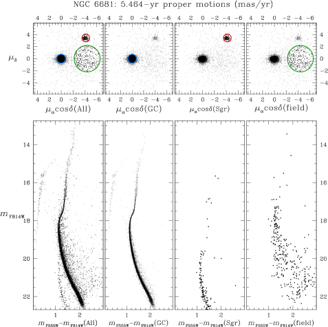
Figure A.1: The upper panels show the VPDs of the relative PMs. In the lower panels the CMDs corresponding to the selections applied in the VPDs are displayed. First column: in the VPD the different populations are indicated with different colors (a sample of cluster members in blue, of Sgr dSph stars in red, of the field in green), but no selection is applied. The corresponding CMD shows the entire PM catalog. Second column: in the VPD cluster members are selected within the blue circle and the corresponding CMD displays only well-defined cluster evolutionary sequences. Third column: Sgr dSph selection within the red circle and corresponding CMD. Fourth column: the selection in the VPD (in green) of the bulk-motion of field stars and their location on the CMD.

1. The cluster population is identified by the clump of stars at (0,0) ${\rm mas\,yr^{-1}}$. By selecting stars within the blue circle in the second upper panel, a clean CMD of the cluster is obtained (second lower panel of Fig. A.1).

2. A secondary clump of stars is located at roughly $(-4,3.5)$ ${\rm mas\,yr^{-1}}$. Stars selected within the red circle in the third upper panel of Fig. A.1 define in the CMD (the third lower panel) a sequence significantly fainter than that defined by cluster stars. Therefore, these stars belong to a population that is both kinematically and photometrically different from that of the cluster. This population appears uniformly distributed across the FoV of our observations and thus it can be associated to the Sgr dSph, whose main body is located in the background of NGC 6681.

3. A much sparser population of stars is centered around $(-4.5,0)$ ${\rm mas\,yr^{-1}}$. The bulk of this population is highlighted with the green circle in the last upper panel of Fig. A.1. The corresponding CMD suggests that this is essentially due to fore/background sources.

A.1.3 Absolute reference frame

In order to measure absolute PMs, an absolute zero point is required. The best option to define this zero point is to use extragalactic sources, since they are essentially stationary on account of their enormous distances. This method has already been adopted in several previous works, such as Dinescu et al. (1999), Bellini et al. (2010), and Sohn et al. (2012). In order to find extragalactic sources we first tried to use the Nasa Extragalactic Database (NED) but no sources in our FoV were reported. This is due to the strong incompleteness of of the NED catalog in the innermost regions of dense stellar systems. We then performed a careful visual inspection of our images. Thirty-one galaxies were identified by eye, but only 11 of them have point-like nuclei and thus are successfully fitted by the adopted PSF. Out of these, we selected only the 5 galaxies with an associated QFIT value (a parameter which describes how well the adopted PSF fits the brightness profile of the source, see Anderson & King 2006 for details) smaller than $0.6$: this was necessary to guarantee a measurement of the source centroid accurate enough to provide a precise determination of the zero point for the absolute PMs. Figure A.2 shows how these galaxies appear in the F814W band.

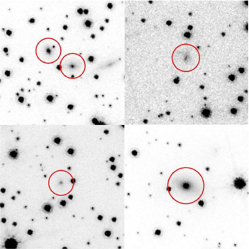
Figure A.2: The five selected background galaxies as they appear in the F814W images. They differ from the stellar sources since their light is more diffuse across the surrounding pixels. Their point-like nuclei allow us to accurately determine their centroid and thus to obtain a precise measure of their relative proper motions.

The selected galaxies are located very close to each other in the relative-PM VPD (Fig. A.3), as expected for distant sources. Therefore, we defined the zero-point of the absolute reference frame as the weighted mean of their relative PMs (see the blue dot in Figure A.3):

$$(\mu_{\alpha}\cos\delta,\mu_{\delta})_{{\rm gals}}=(-1.58\pm 0.18,4.57\pm 0.16)\leavevmode\nobreak\ {\rm mas\,yr^{-1}},$$ (I)

as measured with respect to the mean NGC 6681 motion derived in Section A.1.2. The uncertainties correspond to the error on the calculated weighted means.

A.1.4 NGC 6681

In order to measure the absolute PM of NGC 6681 we selected only stars within $1.0$ ${\rm mas\,yr^{-1}}$from the cluster mean motion and in the magnitude interval $17.5<$m${}_{{\rm F555W}}<22.5$ mag. We iteratively refined the selection by applying a $3\sigma$ rejection and re-calculating the barycenter of the PMs as the weighted mean value of the PMs of the selected stars, until the difference between two subsequent steps was smaller than $0.01$ ${\rm mas\,yr^{-1}}$. After the last iterative step, a total of $N_{clu}=14\,030$ stars survived the selection criteria. We used the sum in quadrature between each single measurement error and the velocity dispersion of the cluster $\sigma_{v}=0.12$ mas/yr (based on the line-of-sight velocity dispersion and distance given by Harris 1996) as weights. To estimate the error $\Delta PM$ on the weighted mean PM in each coordinate we use the standard error-in-the-mean, i.e., the dispersion of the surviving stars around the weighted mean PM, divided by $\sqrt{(}N_{\rm clu}-1)$. This includes scatter from the internal dispersion of NGC 6681 stars, which therefore does not need to be estimated explicitly. We find that the resulting error $\Delta PM$ is negligible compared to the error on the absolute reference frame. Therefore, the latter dominates the uncertainty on the final absolute PM of NGC 6681, which is:

$$(\mu_{\alpha}\cos\delta,\mu_{\delta})=(1.58\pm 0.18,-4.57\pm 0.16)\leavevmode\nobreak\ {\rm mas\,yr^{-1}}.$$ (II)

The PM derived here can be combined with the known distance and line-of-sight velocity of NGC 6681 from Harris (1996), to determine the motion of the cluster in the Galactocentric rest frame. Using the same formalism, conventions, and solar motion as in van der Marel et al. (2012), this yields $(V_{X},V_{Y},V_{Z})=(203\pm 2,111\pm 9,-179\pm 7)$ km s^-1. This corresponds to a total Galactocentric velocity $|{\vec{V}}|=292\pm 5$ km s^-1. This significantly exceeds the central velocity dispersion $\sigma\approx 120$ km s^-1 of the Milky Way’s spheroidal components (e.g., Deason et al. 2012). Hence, NGC 6681 must spend most of the time along its orbit at significantly larger distances from the Galactic Center than its current distance of $2.2$ kpc (Harris 1996).

A.1.5 Sagittarius Dwarf Galaxy

In order to determine the absolute PM of the Sgr dSph we basically followed the same procedure previously described for NGC 6681. In setting the weights for the PM averaging, we used the dispersion $\sigma_{v}\sim 0.3$ ${\rm mas\,yr^{-1}}$implied by Figure 6. This includes both contributions from the internal velocity dispersion of the Sgr dSph (see e.g. Frinchaboy et al. 2012), and unquantified systematic errors. We selected stars within $1.0$ ${\rm mas\,yr^{-1}}$from the Sgr dSph mean motion and in the interval $17.5<$m${}_{{\rm F555W}}<23.5$, which is one magnitude fainter with respect to the case of NGC 6681, since most of the Sgr dSph stars belong to its faint MS. The resulting absolute PM is:

$$(\mu_{\alpha}\cos\delta,\mu_{\delta})=(-2.54\pm 0.18,-1.19\pm 0.16)\leavevmode\nobreak\ {\rm mas\,yr^{-1}}.$$ (III)

We compared this value with previous estimates. With the aim of reconstructing the kinematical history of this galaxy and to predict its evolution in a triaxial Milky Way halo, Law & Majewski (2010) built a N-body model able to reproduce most of the system’s observed properties. In the Law & Majewski model, the Sgr dSph has a Galactocentric motion $(V_{X},V_{Y},V_{Z})=(230,-35,195)$ km s^-1, corresponding to a total velocity $|{\vec{V}}|=304$ km s^-1. The absolute PM predicted by the model is ($\mu_{\alpha}\cos\delta,\mu_{\delta})=(-2.45,-1.30$) ${\rm mas\,yr^{-1}}$(light green dot in Figure A.3). An estimate of the absolute PM of the Sgr dSph based on HST data has been recently presented by Pryor et al. (2010). The authors used foreground Galactic stellar populations as reference frame and they determined an absolute PM of ($\mu_{\alpha}\cos\delta,\mu_{\delta})=(-2.37\pm 0.2,-1.65\pm 0.22$) ${\rm mas\,yr^{-1}}$, which is shown as a magenta ellipse in Figure A.3. A ground-based estimate of the absolute PM of the Sgr dSph was presented by Dinescu et al. (2005). Using the Southern Proper Motion Catalog 3 they determined that $(\mu_{\alpha}\cos\delta,\mu_{\delta})=(-2.83\pm 0.20,-1.33\pm 0.20)$ ${\rm mas\,yr^{-1}}$, which is shown as the dark green ellipse in Figure A.3. These previous estimates are in rough agreement with the value determined here.

It is worth noting, however, that these other determinations are not directly comparable with ours, since they refer to different regions of the Sgr dSph. Indeed, this has two possible effects. The first one is that possible internal motions, such as rotation, could translate into different mean motions, thus introducing a systematic effect. This should not be a problem for the Sgr dSph, since this galaxy does not show any evidence of rotation (Peñarrubia et al. 2011). The second effect is that if the whole galaxy has a 3D velocity vector different from zero, then the observed PMs for different pointings are not the same, because of perspective effects due to the imperfect parallelism between the lines of sight (van der Marel et al. 2002). Since the Sgr dSph is a nearby galaxy, this effect could be relevant and we calculated the correction to apply (as in van der Marel & Guhathakurta 2008) in order to obtain comparable estimates at the center of mass of the Sgr dSph.

Under the hypothesis that the center of mass of the Sgr dSph is moving as the Law & Majewski (2010) prediction, our perspective-corrected PM measurement becomes ($\mu_{\alpha}\cos\delta,\mu_{\delta})=(-2.56\pm 0.18,-1.29\pm 0.16$) ${\rm mas\,yr^{-1}}$. The corrected Pryor et al. (2010) estimate becomes ($\mu_{\alpha}\cos\delta,\mu_{\delta})=(-2.37\pm 0.20,-1.63\pm 0.22$) ${\rm mas\,yr^{-1}}$, and the corrected Dinescu et al. (2005) estimate becomes $(\mu_{\alpha}\cos\delta,\mu_{\delta})=-2.83\pm 0.20,-1.56\pm 0.20)$ ${\rm mas\,yr^{-1}}$. Thus our measurement is consistent with the previous observations. The weighted average of all observational estimates of the center-of-mass PM of the Sgr dSph is $(\mu_{\alpha}\cos\delta,\mu_{\delta})=(-2.59\pm 0.11,-1.45\pm 0.11)$ ${\rm mas\,yr^{-1}}$. This is consistent with the theoretical model of Law & Majewski (2010), once the uncertainties on transforming that into a PM value (e.g., from uncertainties in the distance and solar motion) are taken into account as well. Therefore, our measurement is consistent within about a $1\sigma$ uncertainty both with theoretical predictions (Law & Majewski 2010) and the previous HST observations (Pryor et al. 2010).

A.1.6 Field

We compared the absolute PMs of Field stars in our catalog with those predicted in the same region of sky by the Besançon Galactic model (Robin et al. 2003). We generated a simulation over a 0.01 square degrees ($6\mbox{${}^{\prime}$}\times 6\mbox{${}^{\prime}$}$) FoV around the center of NGC 6681 ($l=2$°​.$85$, $b=-12$°​.$51$) and 50 kpc deep. To minimize any possible bias, we have constructed a sample as similar as possible to the observed stars, based on a comparison between the observed and the simulated CMDs. Simulated field stars were selected within the magnitude range: $17.5<$m${}_{{\rm F555W}}<22.5$ mag and (m${}_{{\rm F555W}}-$m_F814W)$>1.5$ mag and 1378 stars survived these criteria. The average predicted motion is shown in Figure A.3 as a cyan ellipse, which corresponds to ($\mu_{\alpha}\cos\delta,\mu_{\delta})=(-0.91\pm 0.08,-2.39\pm 0.09$) ${\rm mas\,yr^{-1}}$.

Field stars in our observed catalog were selected following the same color and magnitude cuts. We also required these stars to have PM errors smaller than $0.2$ ${\rm mas\,yr^{-1}}$in each coordinate. Finally, we excluded those stars within $1.8$ ${\rm mas\,yr^{-1}}$of the cluster mean motion and within $1.0$ ${\rm mas\,yr^{-1}}$of the Sgr dSph mean motion. We iteratively removed field stars in symmetric locations with respect to the Sgr dSph and NGC 6681 exclusions in order to better define the mean motion of the Field population and adjusted the weighted mean motion after each iteration (thus following the method described by Anderson & van der Marel 2010 for the determination of the center of $\omega$ Cen). The 281 selected field stars used for the final estimate are shown as black crosses in Figure A.3. Since these stars display a large scatter in the VPD due to their velocity dispersion and not to their random errors, in this case we computed a statistically more appropriate $3\sigma$-clipped unweighted mean motion. It is shown as a blue ellipse in Figure A.3 and its value is:

$$(\mu_{\alpha}\cos\delta,\mu_{\delta})=(-1.21\pm 0.27,-4.39\pm 0.26){\rm mas\,yr^{-1}}.$$ (IV)

Our PM measurement is similar to the prediction of the Besançon model, in that it points in the same direction on the sky (see Figure A.3). However, the sizes of the PM vectors are not formally consistent to within the random errors. Since our measurements for Sgr dSph stars are entirely consistent with both previous measurements and theoretical predictions, this cannot be due to systematic errors in our measurements (which would affect all point sources equally). Instead, the mismatch is most likely due to shortcomings in the Besançon models. In particular, for pointings this close to the Galactic Plane, the model predicted PM distribution is likely to depend sensitively on the adopted dust extinction model, which is poorly constrained observationally. Also, the model predicted PM distribution depends on the solar motion in the Milky Way, which continues to be debated (e.g., McMillan 2011; Bovy et al. 2012).

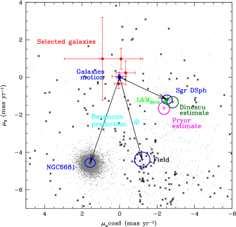
Figure A.3: VPD of the absolute PMs. The red dots indicate the selected background galaxies, whose mean motion corresponds to the zero point of the VPD. The blue ellipses are centered on the measured absolute PMs of the three populations (marked with a blue cross) and their size corresponds to the calculated 68.3% confidence region. The black arrows indicate their absolute PM vectors. In the proximity of the Sgr dSph estimate, the PM value predicted by Law & Majewski (2010) is shown as a light green dot, while the Pryor et al. (2010) and Dinescu et al. (2005) measurements and their 68.3% confidence regions are shown as magenta and dark green ellipses, respectively. Finally, the cyan ellipse describes the prediction on the PM of the field population by the Besançon model, which differs from our estimate obtained using the stars in the same magnitude and color range (marked with black crosses, see the text for the selection criteria).

A.2 Double Blue Straggler sequences in GCs: the case of NGC 362

The second case under study concerns the BSS population of the Galactic GC NGC 362. A series of suitably planned photometric observations with the HST and the analysis of the proper-motion-selected CMD allowed us to discover two distinct sequences of BSS, a rare feature observed only in one other GC in the Galaxy (namely M30, Ferraro et al 2009b). All the details regarding this study can be found in Dalessandro et al. (2013).

A.2.1 General context

Among the large variety of exotic objects (like X-ray binaries, MSPs, etc.) which populate the dense environment of Galactic GCs (see Bailyn 1995, Paresce et al. 1992, Bellazzini et al. 1995, Ferraro et al. 2001, 2003, 2006c, Ransom et al. 2005, Freire et al. 2008), BSS surely represent the most numerous and ubiquitous population. Indeed, BSS have been detected in any properly observed stellar system (GCs, see Fusi Pecci et al. 1992, Ferraro et al. 1992 Piotto et al. 2004; open clusters – Mathieu & Geller 2009 – dwarf galaxies – Mapelli et al. 2009). BSS are brighter and bluer than the MSTO, thus mimicking a population significantly younger than normal cluster stars. Indeed, observations demonstrated that they have masses larger than that of MSTO stars ($m=1.2-1.7\leavevmode\nobreak\ M_{\odot}$; Shara et al. 1997; Gilliland et al. 1998; De Marco et al. 2004, Fiorentino et al. 2014). However, stellar evolution models predict that single stars of comparable mass generated at the epoch of the cluster formation should have already evolved away from the MS; thus some mechanisms must have been at work to increase the mass of these objects in their relatively recent past ($2-3$ Gyr ago; Sills et al. 2002).

Two main formation scenarios for BSS have been proposed over the years: mass transfer (MT-BSS) and direct collision (COL-BSS). The collisional formation channel between two single stars was theorized for the first time by Hills & Day (1976). Following works (Lombardi et al. 2002; Fregeau et al. 2004) showed that BSS may form also via collision between binary-single and binary-binary systems. In the mass transfer scenario (McCrea 1964), the primary star transfers material to the secondary one through the inner Lagrangian point when its Roche Lobe is filled. In this picture the secondary star becomes a more massive MS star (with a lifetime increased by a factor of 2 with respect to a normal star of the same mass – McCrea 1964) with an envelope rich of gas accreted from the donor star. Chemical anomalies are expected for MT-BSS (Sarna & De Greve 1996), since the accreted material (currently settled at the BSS surface) could come from the inner region of the donor star, where nuclear processing occurred. Spectroscopic results supporting the occurrence of the MT formation channel in a few BSS have been recently obtained (Ferraro et al. 2006a; Lovisi et al. 2013). Conversely, surface chemical anomalies are not expected for COL-BSS (Lombardi et al. 1995), since no significant mixing should occur between the inner core and the outer envelope.

In GCs, where the stellar density significantly varies from the center to the external regions, BSS can be generated by both processes (Fusi Pecci et al. 1992, Ferraro et al 1995). Recent works suggested that MT is the dominant formation mechanism in low density clusters (Sollima et al. 2008) and possibly also in high-density clusters (Knigge et al. 2009). However the discovery of two distinct sequences of BSS in M 30 (Ferraro et al. 2009b) clearly separated in color further supports the possibility that both formation channels can coexist within the cluster core. In fact the blue BSS sequence is nicely reproduced by collisional models (Sills et al 2009), while the red one is compatible with binary systems undergoing MT (see Tian et al. 2006). The origin of the double sequence might be possibly related to the core-collapse process that can trigger the formation of both red and blue BSS, enhancing the probability of collisions and boosting the mass-transfer process in relatively close binaries. Given the evolutionary time-scales for stars in the BSS mass range, the fact that the two sequences are still well distinguishable is a clear indication that core collapse occurred no more than $1-2$ Gyr ago.

In order to further explore the link between the presence of a double sequence of BSS and the occurrence of core collapse, we acquired HST images with the WFC3 for a sample of suspected post-core collapse GGCs. Here we report on the discovery of the second case of a BSS double sequence in NGC 362 .

A.2.2 Observations and Data analysis

In the present work we used data acquired with the UVIS channel of the WFC3 on 2012 April 13 (Proposal ID: 12516; PI: Ferraro). The dataset is composed of fourteen exposures obtained through the F390W (hereafter U) filter, each one with an exposure time $t_{\rm exp}=348$ sec, ten F555W (V) images with $t_{\rm exp}=150$ sec and fifteen F814W (I) frames with $t_{\rm exp}=348$ sec. Each pointing is dithered by a few pixels in order to allow a better subtraction of CCD defects, artifacts and false detections. The data reduction follows the same procedure described in Chapter 2.

As evident in Figure A.4, the CMD of NGC 362 is contaminated by fore and background Galaxy stars and even more strongly by the Small Magellanic Cloud (SMC) populations. In particular the MS of the SMC defines a quite clear sequence at $V>20$ and $0<(U-I)<2$. In order to evaluate the level of contamination in the direction of the cluster, we performed the already described relative PM analysis. For this purpose we complemented our HST WFC3 images with a first epoch data-set consisting of WFC/ACS images obtained in June 2006 (Prop ID 10775; PI: Sarajedini). Also in this case, we repeated the procedure already followed in Chapter 2.

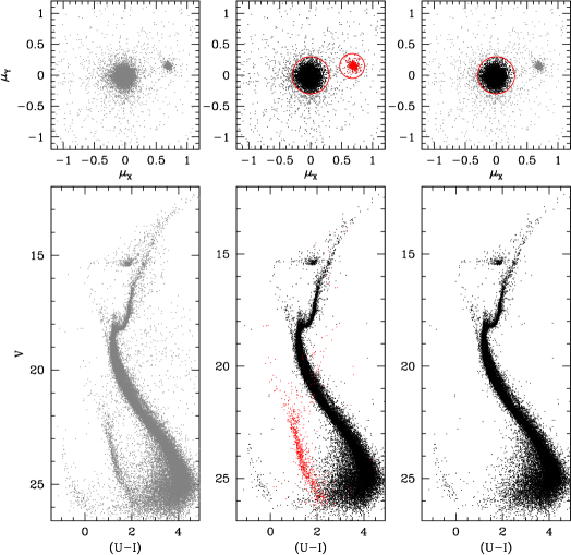
Figure A.4: Upper panels. In the leftmost panel VPDs in pixel/yr of all the stars identified in common between the first and second epoch data sets. In the middle panel the cluster and the SMC populations are selected in black and red respectively. In the rightmost panel only cluster member are selected. Lower panels. From left to right, (V,U-I) CMDs for all the detected stars, for stars with a high cluster membership probability and SMC selected stars (red dots), and for cluster members only.

The upper panels of Figure A.4 present the VPD obtained, where we can distinguish two main sub-populations. The first and dominant one, centered at ($\mu_{X}=0$ pixel yr^-1, $\mu_{Y}=0$ pixel yr^-1) is, by construction, the cluster population. The second, at ($\mu_{X}=0.7$ pixel yr^-1, $\mu_{Y}=0.2$ pixel yr^-1) is instead populated by the SMC stars. The separation between the two components appears clearly in the (V,U-I) CMDs as shown in the lower panels of Figure A.4. In Figure A.5, we show the VPD at different magnitude levels. As expected, the population belonging to the SMC starts to appear in the VPD diagram for $V>20$. In addition the distribution of NGC 362 and SMC gets broader as a function of increasing magnitudes, because of the increasing uncertainties on the centroid positions of faint stars. The same behavior is visible at bright magnitudes ($V<17$) because of non-linearity and saturation problems.

To build a clean sample of stars with a high membership probability, we defined in the VPD and for each magnitude bin a different fiducial region centered on ($\mu_{X}=0$ pixel yr^-1, $\mu_{Y}=0$ pixel yr^-1). The fiducial regions have radii of $2\times\sigma$, where $\sigma$ is the dispersion of fiducial member stars, i.e. those with a distance $r<0.3$ pixel yr^-1 from ($\mu_{X}=0$ pixel yr^-1, $\mu_{Y}=0$ pixel yr^-1) (see the member selection in the upper panels of Figure A.4). It is worth noting that slightly different criteria for the membership selection do not appreciably affect the results about the BSS population.

A.2.3 The BSS double sequence

Given its observed density profile that shows a moderate cusp in the central region of the cluster (see details in Dalessandro et al. 2013), NGC 362 is suspected to have started the core collapse process. This makes it particularly interesting in the context of the working hypothesis proposed by Ferraro et al. (2009b) that clusters undergoing the core-collapse process could develop a double BSS sequence. For this reason, the BSS population of NGC 362 has been analyzed first in the (V,V-I) CMD, in order to perform a direct comparison with the observations of M 30 (Ferraro et al. 2009b). Following the approach adopted in previous papers (Lanzoni et al. 2007a,b; Dalessandro et al. 2008a,b) we selected BSS candidates by defining a box which roughly selects stars brighter and bluer than the TO point, corresponding to $V_{TO}\sim 19$ and $(V-I)_{\rm TO}\sim 0.7$. As usual, in our selection we tried to avoid possible contamination of blends from the SGB, TO region, and the saturation limit of the deep exposures (dashed line in Figure A.5). With these limits 65 candidates BSS have been identified. We emphasize that the selection criteria are not a critical issue here, since the inclusion or exclusion of a few stars does not affect in any way the results of this work. The selected BSS are shown in the zoomed region of the CMD in Figure A.6. At a close look it is possible to distinguish two almost parallel and similarly populated sequences, separated by about $\Delta V\sim 0.4$ and $\Delta(V-I)\sim 0.15$. Such a feature resembles the one observed in M 30.

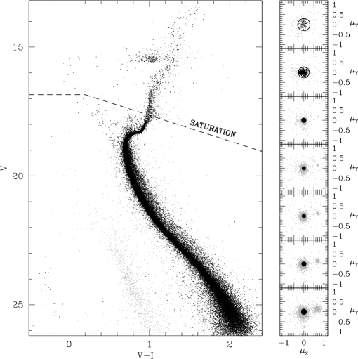
Figure A.5: On the left (V,V-I) CMD of stars in the WFC3 FoV. In black stars selected according to their membership probability, in grey stars excluded on the basis of the criteria highlighted in the VPDs in the right panels. On the right, VPDs at different magnitude levels. The distribution of stars gets broader moving to very faint and bright magnitudes because of the uncertainties on the centroid determination. The black circle represent the $2\sigma$ fiducial region used to clean our sample from non-member stars.

In order to perform a more direct comparison with M 30, we over-plotted two fiducial areas (grey regions in Figure A.6) representative of the color and magnitude distribution of the red and blue BSS populations in that cluster. Differences in distance moduli and reddening have been properly taken into account. Figure A.6 shows that the BSS of NGC 362 nicely fall within the same fiducial regions used to separate the BSS sequences in the case of M 30 (Ferraro et al., 2009b) and only sparsely populate the region between the two. Moreover the BSS population of NGC 362 show luminosity and color extensions similar to the ones observed in M 30. The red sequence appears slightly more scattered than that observed in M 30. This is mainly due to the fact that in the case of NGC 362 a few candidate BSS at $(V-I)\sim 0.6$ have been included into the sample. However, we can safely conclude that, within the photometric uncertainties, the two BSS sequences of NGC 362 well resemble the red and blue BSS sequences of M 30. The blue BSS sample counts 30 stars which are distributed along a narrow and well defined sequence in the (V, V-I) CMD, while the red sequence counts 35 stars. The relative sizes of the two populations is very similar to what found in M 30.

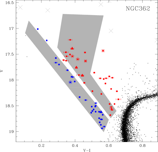
Figure A.6: A zoomed view of the (V,V-I) CMD of NGC 362 on the BSS region. BSS are highlighted as red and blue symbols, and the photometric errors are shown as error bars. The grey areas represent the fiducial loci of the red BSS and blue BSS of M 30 (from Ferraro et al., 2009b). Open squares are SX-Phoenicis found by Szekely et al. (2007). Open pentagons and filled triangles are respectively SX-Phoenicis and WUMa stars identified in this work. Grey crosses are stars excluded for saturation or non linearity problems.

In order to quantify the significance of the bi-modality of the distribution shown in Figure A.6, we used the Gaussian mixture modeling algorithm presented by Muratov & Gnedin (2010) and already described in Chapter 6. We obtain that a unimodal distribution is rejected with a $99.6\%$ probability; hence it is bimodal with a confidence level of $3\sigma$.

We analyzed the spatial distribution of the red and blue BSS populations by looking at their cumulative radial distribution (see Figure A.7). We used SGB stars in the magnitude interval $18<$V$<18.5$ as reference population. Both the red and the blue BSS samples are more centrally concentrated than the reference population. A Kolmogorov-Smirnov test gives a probability $P\sim 10^{-5}$ that they are extracted from the same parent population. Moreover, red BSS are more centrally segregated than the blue ones, with a high ($3\sigma$) confidence level that they are extracted from different populations. In addition, in striking agreement with what found by Ferraro et al. (2009b) in M 30, we do not observe any blue BSS within $5\mbox{${}^{\prime\prime}$}-6\mbox{${}^{\prime\prime}$}$ from $C_{grav}$ and both the blue and red samples completely disappear (within the WFC3 FoV) at distances $r>75\mbox{${}^{\prime\prime}$}$. The observational evidence collected so far leads us to conclude that NGC 362 is the second cluster, after M 30, showing a clear double sequence of BSS.

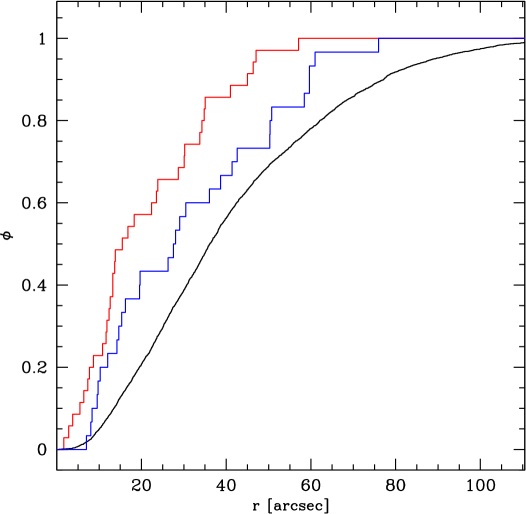
Figure A.7: Cumulative radial distribution of the red and blue BSS samples. In black the distribution of SGB stars, taken as reference population. This analysis is limited to the WFC3 FoV which extends to a distance from $C_{grav}$ $r\sim 100\mbox{${}^{\prime\prime}$}$, corresponding to about $8-9r_{c}$.

A.2.4 Discussion

The accurate HST WFC3 photometry presented in these Sections has revealed the presence of two almost parallel BSS sequences in the core of NGC 362. This represents the second case, after M 30 (Ferraro et al. 2009b), for which a double BSS sequence has been observed. The red and blue BSS populations are well separated in the (V, V-I) CMD by $\Delta$V$\sim 0.4$ and $\Delta$(V-I)$\sim 0.15$, and they nicely overlap with the distribution of BSS shown in Ferraro et al (2009b, see Figures A.6). As in the case of M 30, the red population is significantly more centrally concentrated than the blue one (Figure A.7) and their sizes are very similar. Also the total number of BSS normalized to the total cluster luminosity is basically the same in these two systems. In fact we count, within $r_{t}$ and after field stars subtraction, 77 BSS in NGC 362 which has $L_{V}\sim 2\times 10^{5}L_{\odot}$, and 51 in M 30 (Ferraro et al 2009b) which has instead $L_{V}\sim 10^{5}L_{\odot}$. Ferraro et al. (2009b) argued that blue BSS are likely the result of collisions while red BSS are binary systems in an active phase of mass-transfer. Observational hints supporting this interpretative scenario have been recently shown by Lovisi et al. (2013). A similar approach can be followed to interpret the two sequences in NGC 362. The results are shown in Figure A.8. Indeed the position of the blue sequence in the CMD can be nicely reproduced by a collisional isochrone (Sills et al. 2009) of proper metallicity ([Fe/H]=-1.31) and age $t=0.2$ Gyr and by assuming a distance modulus $(m-M)_{0}=14.68$ and reddening $E(B-V)=0.05$ (Ferraro et al. 1999).

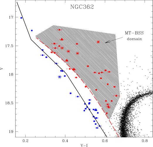
Figure A.8: As in Figure 7, the grey shaded area (here defined as “MT-BSS domain”) approximately indicates the region populated by mass-transfer binaries in M 67 (Tian et al. 2006), "translated" into the CMD of NGC 362. The solid black line is a 0.2 Gyr collisional isochrone (Sills et al. 2009).

In Ferraro et al. (2009b) the position of the red BSS sequence in the CMD has been found to be well reproduced by the lower luminosity boundary defined by the distribution of binary stars with ongoing mass-transfer, as found in Monte Carlo simulations by Tian et al. (2006). This boundary approximately corresponds to the locus defined by the Zero-Age-MS (ZAMS) shifted to brighter magnitudes by $0.75$ mag. The locus obtained for NGC 362 is shown as a red dashed line in Figure A.8. As can be seen, red BSS lie in a sparse area adjacent to the lower boundary in a region that we can call the MT-BSS domain (highlighted in grey in Figure A.8).

In Ferraro et al. (2009b), the presence of two distinct sequences of BSS has been connected to the dynamical state of M 30, in particular to the fact that this cluster might have recently ($1-2$ Gyr ago) experienced the collapse of the core. The dynamical state of NGC 362 is quite debated, and controversial results are found in the literature (Fischer et al. 1993; McLaughlin & van der Marel 2005). The density profile cusp ($\alpha\sim-0.2$, see Dalessandro et al. (2013)) is shallower than typically observed in PCC clusters and could indicate that NGC 362 is on the verge or is currently experiencing the collapse of the core (Vesperini & Trenti 2010). The advanced dynamical age of NGC 362 is also suggested by its monotonic BSS radial distribution. In fact, in the "dynamical clock" classification (Ferraro et al. 2012), NGC 362 belongs (with M 30) to the family of the highly dynamically-evolved clusters (Family III).

On the basis of this observational evidence we can argue that also in the case of NGC 362 the presence of a double BSS sequence could be connected to the advanced dynamical state of the cluster. As in the case of M 30, the fact that we observe two distinct sequences, and in particular a well defined blue one, implies that the event that triggered the formation of the double sequence is recent and short-lived. If this event is connected with the dynamical evolution of the system, it could likely be the collapse of the core (or its initial phase). Indeed, during the collapse, the central density rapidly increases, also enhancing the probability of gravitational encounters (Meylan & Heggie 1997): thus, blue BSS could be formed by direct collisions boosted by the high densities reached in the core, while the red BSS population could have been incremented by binary systems brought to the mass-transfer regime by hardening processes induced by gravitational encounters (McMillan, Hut & Makino 1990; Hurley et al. 2008). Within such a scenario the properties of the blue BSS suggest that the core collapse occurred very recently ($\sim 0.2$ Gyr ago) and over a quite short time scale, of the order of the current core relaxation time ($\sim 10^{8}$ yr; Harris 1996).

References

- Andersen et al. (1999) Andersen, J., et al. 1999, Transactions of the International Astronomical Union, Series A, 24, 36
- Anderson & King (2006) Anderson, J., & King, I., STScI Inst. Sci. Rep. ACS 2006-01 (Baltimore: STScI)
- Anderson (2007) Anderson, J. 2007, Instrument Science Report ACS 2007-08, 12 pages, 8
- Anderson & Bedin (2010) Anderson, J., & Bedin, L. R. 2010, PASP, 122, 1035
- Anderson & van der Marel (2010) Anderson, J., & van der Marel, R. P. 2010, ApJ, 710, 1032
- Anderson et al. (2012) Anderson, J., MacKenty, J., Baggett S., et al. 2012, WFC3/ISR 2012-2013 (Baltimore, MD: STScI)
- Alard (2001) Alard, C. 2001, A&A, 379, L44
- Alcock et al. (1998) Alcock, C., Allsman, R. A., Alves, D. R., et al. 1998, ApJ, 492, 190
- Alonso-García et al. (2011) Alonso-García, J., Mateo, M., Sen, B., Banerjee, M., & von Braun, K. 2011, AJ, 141, 146
- Alves-Brito et al. (2010) Alves-Brito, A., Meléndez, J., Asplund, M., Ramírez, I., & Yong, D. 2010, A&A, 513, A35
- Armandroff & Zinn (1988) Armandroff, T. E., & Zinn, R. 1988, AJ, 96, 92
- Ashman et al. (1994) Ashman, K. M., Bird, C. M., & Zepf, S. E. 1994, AJ, 108, 2348
- Baade (1951) Baade, W. 1951, Publications of Michigan Observatory, 10, 7
- Babusiaux & Gilmore (2005) Babusiaux, C., & Gilmore, G. 2005, MNRAS, 358, 1309
- Babusiaux et al. (2010) Babusiaux, C., Gómez, A., Hill, V., et al. 2010, A&A, 519, A77
- Ballero et al. (2007) Ballero, S. K., Matteucci, F., Origlia, L., & Rich, R. M. 2007, A&A, 467, 123
- Barbuy et al. (1998) Barbuy, B., Bica, E., & Ortolani, S. 1998, A&A, 333, 117
- Bailyn (1995) Bailyn, C. D. 1995, ARA&A, 33, 133
- Beaulieu et al. (2000) Beaulieu, S. F., Freeman, K. C., Kalnajs, A. J., Saha, P., & Zhao, H. 2000, AJ, 120, 855
- Bekki & Freeman (2003) Bekki, K., & Freeman, K. C. 2003, MNRAS, 346, L11
- Bellazzini et al. (1995) Bellazzini, M., Pasquali, A., Federici, L., Ferraro, F. R., & Pecci, F. F. 1995, ApJ, 439, 687
- Bellazzini et al. (1999) Bellazzini, M., Ferraro, F. R., & Buonanno, R. 1999, MNRAS, 307, 619
- Bellazzini et al. (2003) Bellazzini, M., Ferraro, F. R., & Ibata, R. 2003, AJ, 125, 188
- Bellazzini et al. (2008) Bellazzini, M., Ibata, R. A., Chapman, S. C., et al. 2008, AJ, 136, 1147
- Bellini et al. (2009) Bellini, A., Piotto, G., Bedin, L. R., et al. 2009, A&A, 507, 1393
- Bellini et al. (2010) Bellini, A., Bedin, L. R., Piotto, G., et al. 2010, AJ, 140, 631
- Bellini et al. (2010) Bellini, A., Bedin, L. R., Pichardo, B., et al. 2010, A&A, 513, A51
- Bellini et al. (2013) Bellini, A., Anderson, J., Salaris, M., et al. 2013, ApJL, 769, L32
- Bellini et al. (2014) Bellini, A., Anderson, J., van der Marel, R. P., et al. 2014, ApJ, 797, 115
- Bensby et al. (2013) Bensby, T., Yee, J. C., Feltzing, S., et al. 2013, A&A, 549, A147
- Benjamin et al. (2005) Benjamin, R. A., Churchwell, E., Babler, B. L., et al. 2005, ApJL, 630, L149
- Binney et al. (1991) Binney, J., Gerhard, O. E., Stark, A. A., Bally, J., & Uchida, K. I. 1991, MNRAS, 252, 210
- Blommaert & Groenewegen (2007) Blommaert, J. A. D. L., & Groenewegen, M. A. T. 2007, From Stars to Galaxies: Building the Pieces to Build Up the Universe, 374, 193
- Bovy et al. (2012) Bovy, J., Allende Prieto, C., Beers, T. C., et al. 2012, ApJ, 759, 131
- Cao et al. (2013) Cao, L., Mao, S., Nataf, D., Rattenbury, N. J., & Gould, A. 2013, MNRAS, 434, 595
- Canterna (1976) Canterna, R. 1976, AJ, 81, 228
- Cardelli et al. (1989) Cardelli, J. A., Clayton, G. C., & Mathis, J. S. 1989, ApJ, 345, 245
- Carollo et al. (2007) Carollo, C. M., Scarlata, C., Stiavelli, M., Wyse, R. F. G., & Mayer, L. 2007, ApJ, 658, 960
- Carpenter (2001) Carpenter, J. M. 2001, AJ, 121, 2851
- Carraro (2014) Carraro, G. 2014, arXiv:1406.1243
- Carretta et al. (2009) Carretta, E., Bragaglia, A., Gratton, R. G., et al. 2009, A&A, 505, 117
- Carretta et al. (2010a) Carretta, E., Bragaglia, A., Gratton, R., et al. 2010, ApJL, 712, L21
- Carretta et al. (2010b) Carretta, E., Bragaglia, A., Gratton, R. G., et al. 2010, ApJL, 714, L7
- Carretta et al. (2011) Carretta, E., Lucatello, S., Gratton, R. G., Bragaglia, A., & D’Orazi, V. 2011, A&A, 533, A69
- Casetti-Dinescu et al. (2007) Casetti-Dinescu, D. I., Girard, T. M., Herrera, D., et al. 2007, AJ, 134, 195
- Casetti-Dinescu et al. (2010) Casetti-Dinescu, D. I., Girard, T. M., Korchagin, V. I., van Altena, W. F., & López, C. E. 2010, AJ, 140, 1282
- Castelli & Kurucz (2004) Castelli, F., & Kurucz, R. L. 2004, arXiv:astro-ph/0405087
- Cayrel et al. (2004) Cayrel, R., Depagne, E., Spite, M., et al. 2004, A&A, 416, 1117
- Cescutti & Matteucci (2011) Cescutti, G., & Matteucci, F. 2011, A&A, 525, A126
- Clarkson et al. (2008) Clarkson, W., Sahu, K., Anderson, J., et al. 2008, ApJ, 684, 1110
- Clarkson et al. (2011) Clarkson, W. I., Sahu, K. C., Anderson, J., et al. 2011, ApJ, 735, 37
- Cohen et al. (2010) Cohen, J.G., Gould, A., Thompson, I.B., Feltzing, S., Bensby, T., Johnson, J.A., Huang, W., Melendez, J., Lucatello, S., & Asplund, M. 2010, ApJ, 711, L48
- Cohn et al. (2002) Cohn, H. N., Lugger, P. M., Grindlay, J. E., & Edmonds, P. D. 2002, ApJ, 571, 818
- Combes et al. (1990) Combes, F., Debbasch, F., Friedli, D., & Pfenniger, D. 1990, A&A, 233, 82
- D’Antona et al. (2010) D’Antona, F., Ventura, P., Caloi, V., et al. 2010, ApJL, 715, L63
- D’Ercole et al. (2008) D’Ercole, A., Vesperini, E., D’Antona, F., McMillan, S. L. W., & Recchi, S. 2008, MNRAS, 391, 825
- D’Odorico et al. (2006) D’Odorico, S., Dekker, H., Mazzoleni, R., et al. 2006, Proc. SPIE, 6269
- Da Costa et al. (2014) Da Costa, G. S., Held, E. V., & Saviane, I. 2014, MNRAS, 438, 3507
- Dalessandro et al. (2008a) Dalessandro, E., Lanzoni, B., Ferraro, F. R., et al. 2008a, ApJ, 677, 1069
- Dalessandro et al. (2008b) Dalessandro E., Lanzoni B., Ferraro F. R., Vespe F., Bellazzini M., Rood R. T., 2008b, ApJ, 681, 311
- Dalessandro et al. (2014) Dalessandro, E., Massari, D., Bellazzini, M., et al. 2014, ApJL, 791, L4
- Dalessandro et al. (2013) Dalessandro, E., Ferraro, F. R., Massari, D., et al. 2013, ApJ, 778, 135
- De Marco et al. (2004) De Marco, O., Lanz, T., Ouellette, J. A., Zurek, D., & Shara, M. M. 2004, ApJL, 606, L151
- Deason et al. (2012) Deason, A. J., Belokurov, V., Evans, N. W., & An, J. 2012, MNRAS, 424, L44
- Debattista et al. (2013) Debattista, V. P., Roskar, R., Valluri, M., et al. 2013, arXiv:1301.2670
- Decressin et al. (2007) Decressin, T., Charbonnel, C., & Meynet, G. 2007, A&A, 475, 859
- Deg & Widrow (2013) Deg, N., & Widrow, L. 2013, MNRAS, 428, 912
- Dekel et al. (2009) Dekel, A., Sari, R., & Ceverino, D. 2009, ApJ, 703, 785
- Dinescu et al. (1997) Dinescu, D. I., Girard, T. M., van Altena, W. F., Mendez, R. A., & Lopez, C. E. 1997, AJ, 114, 1014
- Dinescu et al. (1999) Dinescu, D. I., Girard, T. M., & van Altena, W. F. 1999, AJ, 117, 1792
- Dinescu et al. (2005) Dinescu, D. I., Girard, T. M., van Altena, W. F., & López, C. E. 2005, ApJL, 618, L25
- Djorgovski (1993) Djorgovski S. 1993, in ASP Conf. Proc. 50, 325
- Dotter et al. (2007) Dotter, A., Chaboyer, B., Jevremović, D., Baron, E., Ferguson, J.-W., Sarajedini, A. & Anderson, J., 2007, AJ, 134, 376
- Eggen et al. (1962) Eggen, O. J., Lynden-Bell, D., & Sandage, A. R. 1962, ApJ, 136, 748
- Elmegreen et al. (2008) Elmegreen, B. G., Bournaud, F., & Elmegreen, D. M. 2008, ApJ, 688, 67
- Faber et al. (2003) Faber, S. et al., 2003, SPIE, 4841, 1657
- Feast (1963) Feast, M. W. 1963, MNRAS, 125, 367
- Ferraro et al. (1992) Ferraro, F. R., Fusi Pecci, F., & Buonanno, R. 1992, MNRAS, 256, 376
- Ferraro et al. (1995) Ferraro, F. R., Fusi Pecci, F., & Bellazzini, M. 1995, A&A, 294, 80
- Ferraro et al. (1999) Ferraro, F. R., Messineo, M., Fusi Pecci, F., et al. 1999, AJ, 118, 1738
- Ferraro et al. (2001) Ferraro, F. R., D’Amico, N., Possenti, A., Mignani, R. P., & Paltrinieri, B. 2001, ApJ, 561, 337
- Ferraro et al. (2003) Ferraro, F. R., Possenti, A., Sabbi, E., et al. 2003, ApJ, 595, 179
- Ferraro et al. (2004) Ferraro, F. R., Sollima, A., Pancino, E., et al. 2004, ApJL, 603, L81
- Ferraro et al. (2006a) Ferraro, F. R., Valenti, E., & Origlia, L. 2006, ApJ, 649, 243
- Ferraro et al. (2006b) Ferraro F. R., Sollima A., Rood R. T., Origlia L., Pancino E., Bellazzini M., 2006b, ApJ, 638, 433
- Ferraro et al. (2006) Ferraro, F. R., Sabbi, E., Gratton, R., et al. 2006, ApJL, 647, L53
- Ferraro et al. (2009) Ferraro, F. R., Dalessandro, E., Mucciarelli, A., et al. 2009, Nature, 462, 483
- Ferraro et al. (2009) Ferraro F. R., et al., 2009, Nature, 462, 1028 (F09)
- Ferraro et al. (2012) Ferraro, F.R. et al., 2012, Nature, 492, 393 (F12)
- Fiorentino et al. (2014) Fiorentino, G., Lanzoni, B., Dalessandro, E., et al. 2014, ApJ, 783, 34
- Fischer et al. (1993) Fischer, P., Welch, D. L., Mateo, M., & Cote, P. 1993, AJ, 106, 1508
- Forbes & Bridges (2010) Forbes, D. A., & Bridges, T. 2010, MNRAS, 404, 1203
- Förster Schreiber et al. (2011) Förster Schreiber, N. M., Shapley, A. E., Genzel, R., et al. 2011, ApJ, 739, 45
- Freeman et al. (2013) Freeman, K., Ness, M., Wylie-de-Boer, E., et al. 2013, MNRAS, 428, 3660
- Fregeau et al. (2004) Fregeau, J. M., Cheung, P., Portegies Zwart, S. F., & Rasio, F. A. 2004, MNRAS, 352, 1
- Freire et al. (2008) Freire, P. C. C., Ransom, S. M., Bégin, S., et al. 2008, ApJ, 675, 670
- Frinchaboy et al. (2012) Frinchaboy, P. M., Majewski, S. R., Muñoz, R. R., et al. 2012, ApJ, 756, 74
- Fulbright (2000) Fulbright, J. P. 2000, AJ, 120, 1841
- Fulbright et al. (2006) Fulbright, J. P., McWilliam, A., & Rich, R. M. 2006, ApJ, 636, 821
- Fulbright et al. (2007) Fulbright, J. P., McWilliam, A., & Rich, R. M. 2007, ApJ, 661, 1152
- Fukugita et al. (1998) Fukugita, M., Hogan, C. J., & Peebles, P. J. E. 1998, ApJ, 503, 518
- Fusi Pecci et al. (1992) Fusi Pecci, F., Ferraro, F. R., Corsi, C. E., Cacciari, C., & Buonanno, R. 1992, AJ, 104, 1831
- Gerhard & Martinez-Valpuesta (2012) Gerhard, O., & Martinez-Valpuesta, I. 2012, ApJL, 744, L8
- Gilliland et al. (1998) Gilliland R. L., Bono G., Edmonds P. D., Caputo F., Cassisi S., Petro L. D., Saha A., Shara M. M., 1998, ApJ, 507, 818
- Girardi et al. (2010) Girardi, L., Williams, B. F., Gilbert, K. M., et al. 2010, ApJ, 724, 1030
- Gonzalez et al. (2011) Gonzalez, O. A., Rejkuba, M., Zoccali, M., et al. 2011, A&A, 530, A54
- Gonzalez et al. (2012) Gonzalez, O. A., Rejkuba, M., Zoccali, M., et al. 2012, A&A, 543, A13
- Grevesse & Sauval (1998) Grevesse, N. & Sauval, A. J., 1998, SSRv, 85, 161
- Gustafsson et al. (2008) Gustafsson, B., Edvardsson, B., Eriksson, K., Jorgensen, U. G., Nordlund, A. & Plez, B., 2008, A&A, 486, 951
- Hammersley et al. (2001) Hammersley, P. L., López-Corredoira, M., & Garzon, F. 2001, Tetons 4: Galactic Structure, Stars and the Interstellar Medium, 231, 81
- Harris (1996) Harris, W. E. 1996, AJ, 112, 1487
- Hill et al. (2011) Hill, V., Lecureur, A., Gómez, A., et al. 2011, A&A, 534, A80
- Hills & Day (1976) Hills J. G., Day C. A., 1976, ApL, 17, 87
- Hinkle et al. (2000) Hinkle, K., Wallace, L., Valenti, J., Harmer, D., 2000, Visible and Near Infrared Atlas of the Arcturus Spectrum 3727-9300 A ed. Kenneth Hinkle, Lloyd Wallace, Jeff Valenti, and Dianne Harmer. (San Francisco: ASP)
- Howard et al. (2008) Howard, C. D., Rich, R. M., Reitzel, D. B., et al. 2008, ApJ, 688, 1060
- Howard et al. (2009) Howard, C. D., Rich, R. M., Clarkson, W., et al. 2009, ApJL, 702, L153
- Hurley et al. (2008) Hurley, J. R., Shara, M. M., Richer, H. B., et al. 2008, AJ, 135, 2129
- Ibata et al. (1994) Ibata, R. A., Gilmore, G., & Irwin, M. J. 1994, Nature, 370, 194
- Ibata et al. (2011) Ibata, R., Sollima, A., Nipoti, C., Bellazzini, M., Chapman, S. C., & Dalessandro, E., 2011, ApJ, 738, 186
- Immeli et al. (2004) Immeli, A., Samland, M., Gerhard, O., & Westera, P. 2004, A&A, 413, 547
- Johnson, Bernat & Krupp (1980) Johnson, H. R., Bernat, A. P., & Krupp, B. M. 1980, ApJS, 42, 501
- Johnson & Pilachowski (2010) Johnson, C. I., & Pilachowski, C. A. 2010, ApJ, 722, 1373
- Johnson et al. (2011) Johnson, C. I., Rich, R. M., Fulbright, J. P., Valenti, E., & McWilliam, A. 2011, ApJ, 732, 108
- Johnson et al. (2012) Johnson, C. I., Rich, R. M., Kobayashi, C., & Fulbright, J. P. 2012, ApJ, 749, 175
- Johnson et al. (2013) Johnson, C. I., Rich, R. M., Kobayashi, C., et al. 2013, ApJ, 765, 157
- Johnson et al. (2014) Johnson, C. I., Rich, R. M., Kobayashi, C., Kunder, A., & Koch, A. 2014, arXiv:1407.2282
- Kappeler et al. (1989) Kappeler, F., Beer, H., & Wisshak, K. 1989, Reports on Progress in Physics, 52, 945
- Kerr & Lynden-Bell (1986) Kerr, F. J., & Lynden-Bell, D. 1986, MNRAS, 221, 1023
- King (1972) King, I.R. 1972, A&A, 19, 166
- Knigge et al. (2009) Knigge, C., Leigh, N., & Sills, A. 2009, Nature, 457, 288
- Kormendy & Kennicutt (2004) Kormendy, J., & Kennicutt, R. C., Jr. 2004, ARA&A, 42, 603
- Kunder et al. (2012) Kunder, A., Koch, A., Rich, R. M., et al. 2012, AJ, 143, 57
- Lanzoni et al. (2007a) Lanzoni, B., Sanna, N., Ferraro, F. R., et al. 2007, ApJ, 663, 1040
- Lanzoni et al. (2007b) Lanzoni B., Dalessandro E., Ferraro F. R., Mancini C., Beccari G., Rood R. T., Mapelli M., Sigurdsson S., 2007b, ApJ, 663, 267
- Lanzoni et al. (2010) Lanzoni, B., Ferraro, F. R., Dalessandro, E., et al. 2010, ApJ, 717, 653
- Law et al. (2005) Law, D. R., Johnston, K. V., & Majewski, S. R. 2005, ApJ, 619, 807
- Law & Majewski (2010) Law, D. R., & Majewski, S. R. 2010, ApJ, 714, 229
- Lee et al. (1999) Lee, Y.-W., Joo, J.-M., Sohn, Y.-J., et al. 1999, Nature, 402, 55
- Liszt & Burton (1980) Liszt, H. S., & Burton, W. B. 1980, ApJ, 236, 779
- Lombardi et al. (1995) Lombardi, J., C., Jr., Rasio, F. A., & Shapiro, S. L. 1995, ApJL, 445, L117
- Lombardi et al. (2002) Lombardi, J. C., Jr., Warren, J. S., Rasio, F. A., Sills, A., & Warren, A. R. 2002, ApJ, 568, 939
- Lovisi et al. (2013) Lovisi, L., Mucciarelli, A., Lanzoni, B., et al. 2013, arXiv:1306.0839
- Majewski et al. (2012) Majewski, S. R., Nidever, D. L., Smith, V. V., et al. 2012, ApJL, 747, L37
- Mapelli et al. (2009) Mapelli, M., Ripamonti, E., Battaglia, G., et al. 2009, MNRAS, 396, 1771
- Marigo et al. (2008) Marigo, P., Girardi, L., Bressan, A., et al. 2008, A&A, 482, 883
- Marino et al. (2009) Marino, A. F., Milone, A. P., Piotto, G., et al. 2009, A&A, 505, 1099
- Marino et al. (2011a) Marino, A. F. et al., 2011, A&A, 532, 8
- Marino et al. (2012) Marino, A. F. et al., 2012, A&A, 541, 15
- Martinez-Valpuesta & Gerhard (2013) Martinez-Valpuesta, I., & Gerhard, O. 2013, ApJL, 766, L3
- Massari et al. (2012) Massari, D., Mucciarelli, A., Dalessandro, E., et al. 2012, ApJL, 755, L32
- Massari et al. (2013) Massari, D., Bellini, A., Ferraro, F. R., et al. 2013, ApJ, 779, 81
- Massari et al. (2014a) Massari, D., Mucciarelli, A., Ferraro, F. R., et al. 2014, ApJ, 791, 101
- Massari et al. (2014b) Massari, D., Mucciarelli, A., Ferraro, F. R., et al. 2014, ApJ, 795, 22
- Mathieu & Geller (2009) Mathieu, R. D., & Geller, A. M. 2009, Nature, 462, 1032
- Matteucci & Brocato (1990) Matteucci, F., & Brocato, E. 1990, ApJ, 365, 539
- Matteucci & Romano (1999) Matteucci, F., & Romano, D. 1999, Ap&SS, 265, 311
- McLaughlin & van der Marel (2005) McLaughlin D.E., van der Marel R.P., 2005, ApJSS, 161, 304
- McLean et al. (1998) McLean, I. S., Becklin, E. E., Bendiksen, O., et al. 1998, Proc. SPIE, 3354, 566
- McMillan et al. (1990) McMillan, S., Hut, P., & Makino, J. 1990, ApJ, 362, 522
- McMillan (2011) McMillan, P. J. 2011, MNRAS, 414, 2446
- McWilliam & Rich (1994) McWilliam, A., & Rich, R. M. 1994, ApJS, 91, 749
- McWilliam & Zoccali (2010) McWilliam, A., & Zoccali, M. 2010, ApJ, 724, 1491
- McCrea (1964) McCrea W. H., 1964, MNRAS, 128, 147
- Meléndez et al. (2008) Meléndez, J., Asplund, M., Alves-Brito, A., et al. 2008, A&A, 484, L21
- Meylan & Heggie (1997) Meylan, G., & Heggie, D. C. 1997, A&A Rev., 8, 1
- Mezger et al. (1999) Mezger, P. G., Zylka, R., Philipp, S., & Launhardt, R. 1999, A&A, 348, 457
- Mezsaros et al. (2012) Meszaros, Sz., Allende Prieto, C., Edvardsson, B., Castelli, F., Garcia Perez, A. E., Gustafsson, B., Majewski, S. R., Plez, B., Schiavon, R., Shetrone, M., & de Vicente, A., 2012, AJ, 144, 120
- Miocchi et al. (2013) Miocchi, P., Lanzoni, B., Ferraro, F. R., et al. 2013, ApJ, 774, 151
- Monaco et al. (2007) Monaco, L., Bellazzini, M., Bonifacio, P., et al. 2007, A&A, 464, 201
- Montegriffo et al. (1998) Montegriffo, P., Ferraro, F. R., Origlia, L. & Fusi Pecci, F., 1998, MNRAS, 297, 872
- Mucciarelli et al. (2009) Mucciarelli, A., Origlia, L., Ferraro, F. R., & Pancino, E. 2009, ApJL, 695, L134
- Mucciarelli (2011) Mucciarelli, A., 2011, A&A, 528, 44
- Mucciarelli et al. (2012) Mucciarelli, A., Bellazzini, M., Ibata, R., Merle, T., Chapman, S. C., Dalessandro, E., & Sollima, A., 2012, MNRAS, 426, 2889
- Mucciarelli et al. (2013) Mucciarelli, A., Pancino, E., Lovisi, L., Ferraro, F. R., & Lapenna, E. 2013, ApJ, 766, 78
- Mucciarelli (2013) Mucciarelli, A. 2013, arXiv:1311.1403
- Munoz, Geisler & Villanova (2013) Munoz, C., Geisler, D., & Villanova, S., 2013, MNRAS, 433, 2006
- Muratov & Gnedin (2010) Muratov, A. L., & Gnedin, O. Y. 2010, ApJ, 718, 1266
- Nataf et al. (2010) Nataf, D. M., Udalski, A., Gould, A., Fouqué, P., & Stanek, K. Z. 2010, ApJL, 721, L28
- Nataf & Gould (2012) Nataf, D. M., & Gould, A. P. 2012, ApJL, 751, L39
- Nassau & Blanco (1958) Nassau, J. J., & Blanco, V. M. 1958, ApJ, 128, 46
- Neckel & Labs (1984) Neckel, H., & Labs, D., 1984, SoPh, 90, 205
- Ness et al. (2013a) Ness, M., Freeman, K., Athanassoula, E., et al. 2013, MNRAS, 430, 836
- Ness et al. (2013b) Ness, M., Freeman, K., Athanassoula, E., et al. 2013, MNRAS, 432, 2092
- Ness et al. (2014) Ness, M., Debattista, V. P., Bensby, T., et al. 2014, ApJL, 787, L19
- Nidever et al. (2012) Nidever, D. L., Zasowski, G., Majewski, S. R., et al. 2012, ApJL, 755, L25
- Noguchi (1999) Noguchi, M. 1999, ApJ, 514, 77
- Norris & Da Costa (1995) Norris, J. E., & Da Costa, G. S. 1995, ApJ, 447, 680
- Origlia, Moorwood & Oliva (1993) Origlia, L., Moorwood, A. F. M., & Oliva, E. 1993, A&A, 280, 536
- Origlia et al. (1997) Origlia, L., Ferraro, F. R., Fusi Pecci, F., & Oliva, E. 1997, A&A, 321, 859
- Origlia, Rich & Castro (2002) Origlia, L., Rich, R. M., & Castro, S. 2002, AJ, 123, 1559
- Origlia et al. (2003) Origlia, L., Ferraro, F. R., Bellazzini, M., & Pancino, E. 2003, ApJ, 591, 916
- Origlia & Rich (2004) Origlia, L., & Rich, R. M. 2004, AJ, 127, 3422
- Origlia et al. (2011) Origlia, L., Rich, R. M., Ferraro, F. R., et al. 2011, ApJL, 726, L20
- Origlia et al. (2013) Origlia, L., Massari, D., Rich, R. M., et al. 2013, ApJL, 779, LL5
- Ortolani et al. (1996) Ortolani, S., Barbuy, B., & Bica, E. 1996, A&A, 308, 733
- Ortolani et al. (2001) Ortolani, S., Barbuy, B., Bica, E., et al. 2001, A&A, 376, 878
- Ortolani et al. (2007) Ortolani, S., Barbuy, B., Bica, E., Zoccali, M., & Renzini, A. 2007, A&A, 470, 1043
- Pancino et al. (2000) Pancino, E., Ferraro, F. R., Bellazzini, M., Piotto, G., & Zoccali, M. 2000, ApJL, 534, L83
- Pancino et al. (2011) Pancino, E., Mucciarelli, A., Sbordone, L., et al. 2011, A&A, 527, A18
- Paresce et al. (1992) Paresce, F., de Marchi, G., & Ferraro, F. R. 1992, Nature, 360, 46
- Pasquini et al. (2002) Pasquini, L., Avila, G., Blecha, A., et al. 2002, The Messenger, 110, 1
- Peñarrubia et al. (2011) Peñarrubia, J., Zucker, D. B., Irwin, M. J., et al. 2011, ApJL, 727, L2
- Pietrinferni et al. (2004) Pietrinferni, A., Cassisi, S., Salaris, M., & Castelli, F. 2004, ApJ, 612, 168
- Pietrinferni et al. (2006) Pietrinferni, A., Cassisi, S., Salaris, M., & Castelli, F. 2006, ApJ, 642, 797
- Piotto et al. (2004) Piotto, G., De Angeli, F., King, I. R., et al. 2004, ApJL, 604, L109
- Platais et al. (1998) Platais, I., Girard, T. M., Kozhurina-Platais, V., et al. 1998, AJ, 116, 2556
- Pryor et al. (2010) Pryor, C., Piatek, S., & Olszewski, E. W. 2010, AJ, 139, 839
- Ramirez & Allende Prieto (2011) Ramirez, I., & Allende Prieto, C., 2011, ApJ, 743, 135
- Rangwala et al. (2009) Rangwala, N., Williams, T. B., & Stanek, K. Z. 2009, ApJ, 691, 1387
- Ransom et al. (2005) Ransom, S. M., Hessels, J. W. T., Stairs, I. H., et al. 2005, Science, 307, 892
- Ransom (2007) Ransom, S. M. 2007, SINS - Small Ionized and Neutral Structures in the Diffuse Interstellar Medium, 365, 265
- Rattenbury et al. (2007) Rattenbury, N. J., Mao, S., Debattista, V. P., et al. 2007, MNRAS, 378, 1165
- Rich (1990) Rich, R. M. 1990, ApJ, 362, 604
- Rich & Origlia (2005) Rich, R. M., & Origlia, L. 2005, ApJ, 634, 1293
- Rich et al. (2007) Rich, R. M., Reitzel, D. B., Howard, C. D., & Zhao, H. 2007, ApJL, 658, L29
- Rich, Origlia & Valenti (2012) Rich, R. M., Origlia, L., & Valenti, E. 2012, ApJ, 746, 59
- Rich (2013) Rich, R. M. 2013, Planets, Stars and Stellar Systems. Volume 5: Galactic Structure and Stellar Populations, 271
- Robin et al. (2003) Robin, A. C., Reylé, C., Derrière, S., & Picaud, S. 2003, A&A, 409, 523
- Ryde et al. (2009) Ryde, N., Edvardsson, B., Gustafsson, B., et al. 2009, A&A, 496, 701
- Saha et al. (2012) Saha, K., Martinez-Valpuesta, I., & Gerhard, O. 2012, MNRAS, 421, 333
- Sanna et al. (2014) Sanna, N., Dalessandro, E., Ferraro, F. R., et al. 2014, ApJ, 780, 90
- Sarna & De Greve (1996) Sarna M. J., De Greve J.-P., 1996, QJRAS, 37, 11
- Saviane et al. (2012) Saviane, I., da Costa, G. S., Held, E. V., Sommariva, V., Gullieuszik, M., Barbuy, B., & Ortolani, S., 2012, A&A, 540, 27
- Sbordone et al. (2004) Sbordone, L., Bonifacio, P., Castelli, F., & Kurucz, R. L., MSAIS, 5, 93
- Schlegel et al. (1998) Schlegel, D. J., Finkbeiner, D. P., & Davis, M. 1998, ApJ, 500, 525
- Schönrich et al. (2010) Schönrich, R., Binney, J., & Dehnen, W. 2010, MNRAS, 403, 1829
- Schuller et al. (2006) Schuller, F., Omont, A., Glass, I. S., et al. 2006, A&A, 453, 535
- Shara, Saffer, & Livio (1997) Shara M. M., Saffer R. A., Livio M., 1997, ApJ, 489, L59
- Shen et al. (2010) Shen, J., Rich, R. M., Kormendy, J., et al. 2010, ApJL, 720, L72
- Sills et al. (2002) Sills, A., Adams, T., Davies, M. B., & Bate, M. R. 2002, MNRAS, 332, 49
- Sills et al. (2009) Sills, A., Karakas, A., & Lattanzio, J. 2009, ApJ, 692, 1411
- Simon & Geha (2007) Simon, J. D., & Geha, M., 2007, ApJ, 670, 313
- Simmerer et al. (2013) Simmerer, J., Ivans, I. I., Filler, D., Francois, P., Charbonnel, C., Monier, R., & James, G., 2013, ApJ, 764, 7L
- Sirianni et al. (2005) Sirianni, M., Jee, M. J., Benítez, N., et al. 2005, PASP, 117, 1049
- Sohn et al. (2012) Sohn, S. T., Anderson, J., & van der Marel, R. P. 2012, ApJ, 753, 7
- Sollima et al. (2004) Sollima, A., Ferraro, F. R., Origlia, L., Pancino, E., & Bellazzini, M. 2004, A&A, 420, 173
- Sollima et al. (2005) Sollima, A., Pancino, E., Ferraro, F. R., et al. 2005, ApJ, 634, 332
- Sollima et al. (2007) Sollima, A., Ferraro, F. R., Bellazzini, M., et al. 2007, ApJ, 654, 915
- Sollima et al. (2008) Sollima, A., Lanzoni, B., Beccari, G., Ferraro, F. R., & Fusi Pecci, F. 2008, A&A, 481, 701
- Soto et al. (2007) Soto, M., Rich, R. M., & Kuijken, K. 2007, ApJL, 665, L31
- Stetson & Pancino (2008) Stetson, P. B., & Pancino, E. 2008, PASP, 120, 1332
- Tian et al. (2006) Tian, B., Deng, L., Han, Z., & Zhang, X. B. 2006, A&A, 455, 247
- Tolstoy et al. (2009) Tolstoy, E., Hill, V., & Tosi, M. 2009, ARA&A, 47, 371
- Tonry & Davis (1979) Tonry, J. & Davis, M., 1979, AJ, 84, 1511
- Toomre (1977) Toomre, A. 1977, ARA&A, 15, 437
- Ubeda & Anderson (2012) Ubeda, L., Anderson, J., STScI Inst. Sci. Rep. ACS 2012-03 (Baltimore: STScI)
- Udalski et al. (2000) Udalski, A., Zebrun, K., Szymanski, M., et al. 2000, Acta Astron., 50, 1
- Uttenthaler et al. (2012) Uttenthaler, S., Schultheis, M., Nataf, D.M., Robin, A.C., Lebzelter, T., & Chen, B. 2012, A&A, 546, 57
- Valcarce & Catelan (2011) Valcarce, A. A. R., & Catelan, M. 2011, A&A, 533, A120
- Valenti et al. (2004) Valenti, E., Ferraro, F. R., & Origlia, L. 2004, MNRAS, 351, 1204
- Valenti et al. (2007) Valenti, E., Ferraro, F. R., & Origlia, L. 2007, AJ, 133, 1287
- Valenti et al. (2010) Valenti, E., Ferraro, F. R., & Origlia, L. 2010, MNRAS, 402, 1729
- Valenti et al. (2013) Valenti, E., Zoccali, M., Renzini, A., et al. 2013, A&A, 559, AA98
- van der Marel et al. (2002) van der Marel, R. P., Alves, D. R., Hardy, E., & Suntzeff, N. B. 2002, AJ, 124, 2639
- van der Marel & Guhathakurta (2008) van der Marel, R. P., & Guhathakurta, P. 2008, ApJ, 678, 187
- van der Marel et al. (2012) van der Marel, R. P., Fardal, M., Besla, G., et al. 2012, ApJ, 753, 8
- van der Marel et al. (2014) van der Marel, R. P., Anderson, J., Bellini, A., et al. 2014, Astronomical Society of the Pacific Conference Series, 480, 43
- van Loon et al. (2003) van Loon, J. T., Gilmore, G. F., Omont, A., et al. 2003, MNRAS, 338, 857
- Ventura et al. (2001) Ventura, P., D’Antona, F., Mazzitelli, I., & Gratton, R. 2001, ApJL, 550, L65
- Verbunt & Hut (1987) Verbunt F. & Hut P. 1987 in Proc. IAU Symp. 125, 187
- Vesperini & Trenti (2010) Vesperini, E., & Trenti, M. 2010, ApJL, 720, L179
- Villanova et al. (2014) Villanova, S., Geisler, D., Gratton, R. G., & Cassisi, S. 2014, arXiv:1406.5069
- von Braun & Mateo (2001) von Braun, K., & Mateo, M. 2001, AJ, 121, 1522
- Yong et al. (2014) Yong, D., Roederer, I. U., Grundahl, F., et al. 2014, MNRAS, 441, 3396
- Willman & Strader (2012) Willman, B., & Strader, J., 2012, AJ, 144, 76
- Wolfe (1971) Wolfe, A. M. 1971, BAAS, 3, 474
- Zhao et al. (1994) Zhao, H., Spergel, D. N., & Rich, R. M. 1994, AJ, 108, 2154
- Zhao & Mao (1996) Zhao, H., & Mao, S. 1996, MNRAS, 283, 1197
- Zinn (1993) Zinn, R., ASP Conf. Ser. 48, The Globular Cluster-Galaxy connection, ed. G.H. Smith & J.P. Brodie (San Francisco, CA:ASP), 38
- Zoccali et al. (2003) Zoccali, M., Renzini, A., Ortolani, S., et al. 2003, A&A, 399, 931
- Zoccali et al. (2008) Zoccali, M., Hill, V., Lecureur, A., et al. 2008, A&A, 486, 177
- Zoccali et al. (2014) Zoccali, M., Gonzalez, O. A., Vasquez, S., et al. 2014, A&A, 562, A66