Abstract

The potential for the measurement of the branching ratio of the Standard Model-like Higgs boson decay into a $\mathup{{}^{\scriptstyle{+}}}\mathup{{}^{\scriptstyle{-}}}$ pair at 1.4 TeV CLIC is analysed. The study is performed using the fully simulated CLIC_ILD detector concept, taking into consideration all the relevant physics and the beam-induced backgrounds. Despite the very low branching ratio of the $\mathup{{{H}}}\to\mathup{{}^{\scriptstyle{+}}}\mathup{{}^{\scriptstyle{-}}}$ decay, we show that the product of the branching ratio times the Higgs production cross section can be measured with a statistical uncertainty of 38$\,\%$, assuming an integrated luminosity of 1.5 $\text{ab}^{-1}$ collected in five years of the detector operation at the 1.4 TeV CLIC with unpolarised beams. With polarised beams (+80$\,\%$, -30$\,\%$), the statistical uncertainty is better than 25$\,\%$

1 Introduction

Measurements of Higgs branching ratios, and consequently Higgs couplings, provide a strong test of the Standard Model (SM) and the physics beyond. Models that could possibly extend SM Higgs sector, such as the Two Higgs Doublet model, the Little Higgs model or the Compositeness models predict Higgs couplings to EW bosons and Higgs Yukawa couplings (coupling-mass linearity) that deviate from the SM predictions [1, 2].

The Compact Linear Collider (CLIC) represents an excellent environment to study properties of the Higgs boson, including the couplings, with a very high precision [3, 4]. Measurement of the rare $\mathup{{{H}}}\to\mathup{{}^{\scriptstyle{+}}}\mathup{{}^{\scriptstyle{-}}}$ decay is particularly challenging because of the very low branching ratio (BR) of $2.14\times 10^{-4}$ predicted in the SM at the Higgs mass of 126 GeV [5]. Presently the search for the $\mathup{{{H}}}\to\mathup{{}^{\scriptstyle{+}}}\mathup{{}^{\scriptstyle{-}}}$ decay at ATLAS including 25 $\text{fb}^{-1}$ of data has yielded an upper limit for BR($\mathup{{{H}}}\to\mathup{{}^{\scriptstyle{+}}}\mathup{{}^{\scriptstyle{-}}}$) of $1.5\times 10^{-3}$ [6]. A similar upper limit was reported by the CMS experiment as well [7]. In the projections for the HL-LHC ATLAS experiment, the SM expectations are $2.3\sigma$ signal significance, or 46$\,\%$ signal counting uncertainty with $300\,\text{fb}^{-1}$ of data, and $7\sigma$ signal significance, or 21$\,\%$ counting uncertainty with $3\,\text{ab}^{-1}$ of collected data [8]. The respective projected significances at CMS are $2.5\sigma$ with $300\,\text{fb}^{-1}$ of data, and $7.9\sigma$ with $3\,\text{ab}^{-1}$ [7]. The measurement at CLIC requires excellent muon identification efficiency and momentum resolution as well as efficient background rejection.

One of the possible staged scenarios of the CLIC construction and operation, optimized for the best physics reach in shortest time with optimal cost, comprises the $350\,\mathrm{GeV}$, $1.4\,\mathrm{TeV}$ and $3\,\mathrm{TeV}$ centre-of-mass (CM) energy stages [9]. In the latter two stages sufficiently large Higgs boson samples are produced via the $\mathup{{{W}}}\mathup{{{W}}}$ fusion process that the measurement of the rare $\mathup{{{H}}}\to\mathup{{}^{\scriptstyle{+}}}\mathup{{}^{\scriptstyle{-}}}$ decay can be performed. The analysis of the $\mathup{{{H}}}\to\mathup{{}^{\scriptstyle{+}}}\mathup{{}^{\scriptstyle{-}}}$ decay at $3\,\mathrm{TeV}$ is presented in Ref. [10]. The analysis at $1.4\,\mathrm{TeV}$ is presented here. The target value of the integrated luminosity at the 1.4$\,\mathrm{TeV}$ stage is $1.5\,\text{ab}^{-1}$. At the instantaneous luminosity of $3.2\times 10^{34}\,\mathrm{cm}^{-2}\,\mathrm{s}^{-1}$ this is achieved in approximately five years of physics operation with 200 running days per year and an effective up-time of 50$\,\%$. This analysis assumes that the total integrated luminosity is collected with the CLIC_ILD detector concept [11]. Unpolarised beams are assumed. With 80$\,\%$ left-handed beam polarisation for the electrons and 30$\,\%$ right handed polarisation for the positrons, the Higgs production through $\mathup{{{W}}}\mathup{{{W}}}$ fusion can be enhanced by a factor 2.34 [4]. A conservative estimate of the final uncertainty in the case that $1.5\,\text{ab}^{-1}$ of data is collected with polarized beams is given at the end.

In this note, the analysis procedure is presented, and statistical and systematic uncertainties of the measurement are determined and discussed. In Section 2 the simulation tools used for the analysis are listed and in Section 3 the CLIC_ILD detector model is briefly described. Signal and background processes and event samples are discussed in Section 4. Tagging of spectator electrons in background processes is described in Section 5. Event preselection, and a final selection using Multivariate Analysis (MVA) is described in Section 6. The di-muon invariant mass fit and the extraction of the statistical uncertainty of the measurement are described in Section 7. A brief discussion of the eventual benefit of a better transverse momentum, $p_{\text{T}}$, resolution is found in Section 8. Systematic uncertainties are discussed in Section 9, followed by the conclusions. In the Appendix, distributions of sensitive variables used in the MVA are shown for all processes before and after the selection.

2 Simulation and analysis tools

The Higgs production through $\mathup{{{W}}}\mathup{{{W}}}$ fusion was simulated in WHIZARD V 1.95 [12] including the CLIC beam spectrum and the Initial State Radiation (ISR). PYTHIA 6.4 [13] was used to simulate the Higgs decay into two muons. The background events were also generated in WHIZARD, using PYTHIA 6.4 to simulate the hadronisation and fragmentation processes. The CLIC luminosity spectrum and the beam induced processes were obtained from GuineaPig 1.4.4 [14].

The interactions with the detector were simulated using the CLIC_ILD detector model within the Mokka simulation package [15], based on Geant4 [16]. A particle flow algorithm [17, 18] was employed in the reconstruction of the final state particles within the Marlin reconstruction framework [19].

The Toolkit for the Multivariate Analysis (TMVA) package [20] was used for the multivariate classification of signal and background events using their kinematic properties.

3 The CLIC_ILD detector model

For CLIC, the ILD detector model [21] has been modified according to specific experimental conditions at CLIC [3]. The subsystems of particular relevance for the present analysis are discussed in the following.

The main tracking device of CLIC_ILD is a Time Projection Chamber (TPC) providing a point resolution in the $r\phi$ plane better than $100\,\mathrm{\upmu m}$. Additional silicon trackers provide precision tracking at the outer surface of the TPC with single point accuracy in the $r\phi$ direction of $7\,\mathrm{\upmu m}$. Vertex detectors closer to the beam-pipe provide resolution better than $3\,\mathrm{\upmu m}$ [3].

High efficiency muon identification is made possible by the iron yoke instrumented with 9 layers of RPC detectors. Muon momenta are determined using the matching tracks in the TPC and the silicon trackers. The efficiency of the muon identification is influenced by the longitudinal segmentation of iron, as well as by the background processes. In the sample of muons from the $\mathup{{{H}}}\to\mathup{{}^{\scriptstyle{+}}}\mathup{{}^{\scriptstyle{-}}}$ decays, muon efficiency is above 99$\,\%$ in the barrel region.

This analysis depends particularly on the muon momentum resolution as it influences the width of the reconstructed di-muon invariant mass peak. The average muon transverse momentum resolution for the signal sample in the barrel region is $\Delta(1/p_{\text{T}})=3.3\times 10^{-5}\,\mathrm{GeV}^{-1}$.

In the very forward region of the CLIC_ILD detector, below 8^∘, no tracking information nor hadronic calorimetry is available. The region between 0.6^∘ and 6.3^∘ is instrumented with two silicon-tungsten sampling calorimeters, LumiCal and BeamCal, for the luminosity measurement, beam-parameter control, as well as tagging of high-energy electrons escaping the main detector at low angles. Together with the very forward segments of ECAL, EM calorimetry is thus available in the region between 0.6^∘ and 8^∘, offering the possibility to suppress four-fermion SM processes with the characteristic low-angle electron signature. The simulation of the very-forward electron tagging is described in Section 5.

Beamstrahlung photons, emitted in beam-beam interactions produce incoherent $\mathup{{{\mathup{{{e}}}}}^{\scriptstyle{+}}}\mathup{{{\mathup{{{e}}}}}^{\scriptstyle{-}}}$ pairs deposited mainly in the low-angle calorimeters. In addition, about 1.3 interactions of Beamstrahlung photons per bunch crossing produce hadrons with a wide angular distribution, influencing the muon momentum resolution due to the occupancy of the inner tracker. These hadrons were included in the analysis by overlaying a map of energy deposits in all detectors, randomly picked from a pre-simulated data set, before the digitisation phase and event reconstruction. Signal and all other background processes are fully simulated in the detector.

4 Event samples

At 1.4 TeV CLIC, the Standard Model Higgs boson is predominantly produced via $\mathup{{{W}}}\mathup{{{W}}}$ fusion (Figures 1 and 2). The effective cross-section for the Higgs production in $\mathup{{{W}}}\mathup{{{W}}}$ fusion assuming CLIC luminosity spectrum is 244 $\,\mathrm{fb}$. The Higgs production cross section above 1 TeV can be determined with a statistical precision better than 1$\,\%$ [4]. Nevertheless, the $\mathup{{{H}}}\to\mathup{{}^{\scriptstyle{+}}}\mathup{{}^{\scriptstyle{-}}}$ signal statistics is expected to be small because the SM prediction for the branching fraction of this particular decay is of the order of $10^{-4}$.

wwfusion (55,33) i1,i2 o1,o2,o3,o4 fermion,label=$\mathup{{{\mathup{{{e}}}}}^{\scriptstyle{-}}}$i1,v1 fermion,label=$\mathup{{{\mathup{{{e}}}}}^{\scriptstyle{+}}}$,label.side=leftv3,i2 fermionv1,o1 fermiono4,v3 boson,label=$\mathup{{{\mathup{{{W}}}}}^{\scriptstyle{-}}}$v1,v2 boson,label=$\mathup{{{\mathup{{{W}}}}}^{\scriptstyle{+}}}$,label.side=leftv3,v2 dashes,label=$\mathup{{{H}}}$v2,v4 fermionv4,o2 fermiono3,v4 v1,v2,v3,v4 ^-o2 ⁺o3 $\mathup{{{\mathup{}}}{}_{\scriptstyle{\!\mathup{{{e}}}}}}$o1 $\mathup{{\overline{{\mathup{}}}}{}_{\scriptstyle{\!\mathup{{{e}}}}}}$o4 l=$g_{\mathup{{{H}}}\mathup{{{W}}}\mathup{{{W}}}}$,l.a=180,l.d=.06wv2 l=$g_{\mathup{{{H}}}\mathup{}\mathup{}}$,l.d=.06wv4

Figure 1: Feynman diagram of the Higgs production in $\mathup{{{W}}}\mathup{{{W}}}$ fusion and the subsequent decay to a pair of muons.

As seen in Figure 2, at 1.4 $\,\mathrm{TeV}$ the Higgs boson is also produced via $\mathup{{{Z}}}\mathup{{{Z}}}$ fusion, with a cross-section equal to about 10$\,\%$ of the Higgs production cross section in $\mathup{{{W}}}\mathup{{{W}}}$ fusion. However, on a test sample of 300 events of $\mathup{{{Z}}}\mathup{{{Z}}}$ fusion followed by the Higgs decay to a pair of muons, not a single event passed the requirements applied in this analysis (Sec. 4.3 and 4.4) implying a selection efficiency smaller than 1.2$\,\%$ (95$\,\%$ CL) for this channel. Therefore this production channel was neglected in the analysis.

The number of simulated signal and background events was chosen so that accurate di-muon invariant mass distributions can be extracted. A sample of 24 000 signal events was simulated, roughly corresponding to a 300-fold of the number of events in 1.5 $\text{ab}^{-1}$ of data. From the signal sample, 6000 events were reserved for the training of the MVA. For each of the background processes, a 2 $\text{ab}^{-1}$ sample was generated, of which 0.5 $\text{ab}^{-1}$ were reserved for the MVA training. The full list of physics and beam-induced backgrounds is given in Table 1.

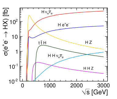
Figure 2: Higgs production cross-sections at different CM energies.

Events with momentum transfer $Q=\sqrt{\left|(p^{\mu}(\mathup{{{e}}}_{out})-p^{\mu}(\mathup{{{e}}}_{in}))^{2}\right|}$ smaller than 4 $\,\mathrm{GeV}$ between the incident and the spectator electron, $\mathup{{{e}}}_{in}$ and $\mathup{{{e}}}_{out}$, respectively, were simulated using the Effective Photon Approximation (EPA). In the EPA approach, the spectator electron is substituted by a quasi-real photon. In the presentation of results of this analysis, such events will be grouped together with the processes involving Beamstrahlung photons with the analogous initial state. Thus, for example, the sample denoted $\mathup{{{\mathup{{{e}}}}}^{\scriptstyle{\pm}}}\mathup{}\to\mathup{{{\mathup{{{e}}}}}^{\scriptstyle{\pm}}}\mathup{{}^{\scriptstyle{+}}}\mathup{{}^{\scriptstyle{-}}}$ contains both the events in which the photon is a Beamstrahlung photon, and the events in which the photon originates from the EPA modelling of the $\mathup{{{\mathup{{{e}}}}}^{\scriptstyle{+}}}\mathup{{{\mathup{{{e}}}}}^{\scriptstyle{-}}}\to\mathup{{{\mathup{{{e}}}}}^{\scriptstyle{+}}}\mathup{{{\mathup{{{e}}}}}^{\scriptstyle{-}}}\mathup{{}^{\scriptstyle{+}}}\mathup{{}^{\scriptstyle{-}}}$ process with small momentum transfer. In this way, processes with roughly similar kinematic characteristics are grouped together.

Table 1 lists the signal and all background processes with their respective cross-sections. Cross sections for processes with spectator electrons were calculated with the cut on momentum transfer $Q>4\,\mathrm{GeV}$, while cross-sections for processes involving initial photons include the cross-sections for the EPA approximation of the processes with spectator electrons for $Q<4\,\mathrm{GeV}$. Beside that, the cross sections for processes $\mathup{{{\mathup{{{e}}}}}^{\scriptstyle{\pm}}}\mathup{}\to\mathup{{{\mathup{{{e}}}}}^{\scriptstyle{\pm}}}\mathup{{}^{\scriptstyle{+}}}\mathup{{}^{\scriptstyle{-}}}$ and $\mathup{{{\mathup{{{e}}}}}^{\scriptstyle{\pm}}}\mathup{}\to\mathup{{{\mathup{{{e}}}}}^{\scriptstyle{\pm}}}\mathup{{{\mathup{}}}{}_{\scriptstyle{\!\mathup{}}}}\mathup{{\overline{{\mathup{}}}}{}_{\scriptstyle{\!\mathup{}}}}\mathup{{}^{\scriptstyle{+}}}\mathup{{}^{\scriptstyle{-}}}$ represent the sum of processes with the electron and the positron in the initial state.

The process $\mathup{{{\mathup{{{e}}}}}^{\scriptstyle{+}}}\mathup{{{\mathup{{{e}}}}}^{\scriptstyle{-}}}\to\mathup{{{\mathup{}}}{}_{\scriptstyle{\!\mathup{{{e}}}}}}\mathup{{\overline{{\mathup{}}}}{}_{\scriptstyle{\!\mathup{{{e}}}}}}\mathup{{}^{\scriptstyle{+}}}\mathup{{}^{\scriptstyle{-}}}$, characterised by the same final state as the signal, as well as by the same distribution of the CM energy in the initial state, represents an irreducible background and can not be substantially suppressed before the invariant mass fit. The process $\mathup{}\mathup{}\to\mathup{{{\mathup{}}}{}_{\scriptstyle{\!\mathup{}}}}\mathup{{\overline{{\mathup{}}}}{}_{\scriptstyle{\!\mathup{}}}}\mathup{{}^{\scriptstyle{+}}}\mathup{{}^{\scriptstyle{-}}}$ has a similar final state, but a different CM energy distribution in the initial state, since it involves Beamstrahlung or EPA photons rather than electrons. This leads to a different distribution of the boost of the di-muon system, as well as of the helicity angle, allowing separation from the signal to some extent (Section 6.2).

The four-fermion production process $\mathup{{{\mathup{{{e}}}}}^{\scriptstyle{+}}}\mathup{{{\mathup{{{e}}}}}^{\scriptstyle{-}}}\to\mathup{{{\mathup{{{e}}}}}^{\scriptstyle{+}}}\mathup{{{\mathup{{{e}}}}}^{\scriptstyle{-}}}\mathup{{}^{\scriptstyle{+}}}\mathup{{}^{\scriptstyle{-}}}$ is realised dominantly through the two-photon exchange mechanism and it fakes the missing energy signature of the signal in events in which electron spectators are emitted at angles smaller than 8^∘. For that reason, the tagging of EM showers at low angles (see Section 5) is applied. The processes $\mathup{{{\mathup{{{e}}}}}^{\scriptstyle{\pm}}}\mathup{}\to\mathup{{{\mathup{{{e}}}}}^{\scriptstyle{\pm}}}\mathup{{}^{\scriptstyle{+}}}\mathup{{}^{\scriptstyle{-}}}$ and $\mathup{{{\mathup{{{e}}}}}^{\scriptstyle{\pm}}}\mathup{}\to\mathup{{{\mathup{{{e}}}}}^{\scriptstyle{\pm}}}\mathup{{{\mathup{}}}{}_{\scriptstyle{\!\mathup{}}}}\mathup{{\overline{{\mathup{}}}}{}_{\scriptstyle{\!\mathup{}}}}\mathup{{}^{\scriptstyle{+}}}\mathup{{}^{\scriptstyle{-}}}$ are suppressed by EM shower tagging as well (see Table 2).

Process	$\sigma(\,\mathrm{fb})$
$\mathup{{{\mathup{{{e}}}}}^{\scriptstyle{+}}}\mathup{{{\mathup{{{e}}}}}^{\scriptstyle{-}}}\to\mathup{{{H}}}\mathup{}\mathup{}$, $\mathup{{{H}}}\to\mathup{{}^{\scriptstyle{+}}}\mathup{{}^{\scriptstyle{-}}}$	0.0522
$\mathup{{{\mathup{{{e}}}}}^{\scriptstyle{+}}}\mathup{{{\mathup{{{e}}}}}^{\scriptstyle{-}}}\to\mathup{{{\mathup{}}}{}_{\scriptstyle{\!\mathup{{{e}}}}}}\mathup{{\overline{{\mathup{}}}}{}_{\scriptstyle{\!\mathup{{{e}}}}}}\mathup{{}^{\scriptstyle{+}}}\mathup{{}^{\scriptstyle{-}}}$	129
$\mathup{{{\mathup{{{e}}}}}^{\scriptstyle{+}}}\mathup{{{\mathup{{{e}}}}}^{\scriptstyle{-}}}\to\mathup{{{\mathup{{{e}}}}}^{\scriptstyle{+}}}\mathup{{{\mathup{{{e}}}}}^{\scriptstyle{-}}}\mathup{{}^{\scriptstyle{+}}}\mathup{{}^{\scriptstyle{-}}}$	24.5∗
$\mathup{{{\mathup{{{e}}}}}^{\scriptstyle{\pm}}}\mathup{}\to\mathup{{{\mathup{{{e}}}}}^{\scriptstyle{\pm}}}\mathup{{}^{\scriptstyle{+}}}\mathup{{}^{\scriptstyle{-}}}$	1098∗
$\mathup{{{\mathup{{{e}}}}}^{\scriptstyle{\pm}}}\mathup{}\to\mathup{{{\mathup{{{e}}}}}^{\scriptstyle{\pm}}}\mathup{{{\mathup{}}}{}_{\scriptstyle{\!\mathup{}}}}\mathup{{\overline{{\mathup{}}}}{}_{\scriptstyle{\!\mathup{}}}}\mathup{{}^{\scriptstyle{+}}}\mathup{{}^{\scriptstyle{-}}}$	30
$\mathup{}\mathup{}\to\mathup{{{\mathup{}}}{}_{\scriptstyle{\!\mathup{}}}}\mathup{{\overline{{\mathup{}}}}{}_{\scriptstyle{\!\mathup{}}}}\mathup{{}^{\scriptstyle{+}}}\mathup{{}^{\scriptstyle{-}}}$	162
$\mathup{{{\mathup{{{e}}}}}^{\scriptstyle{+}}}\mathup{{{\mathup{{{e}}}}}^{\scriptstyle{-}}}\to\mathup{{{\mathup{{{e}}}}}^{\scriptstyle{+}}}\mathup{{{\mathup{{{e}}}}}^{\scriptstyle{-}}}\mathup{{{\mathup{}}}{}_{\scriptstyle{\!\mathup{}}}}\mathup{{\overline{{\mathup{}}}}{}_{\scriptstyle{\!\mathup{}}}}\mathup{{}^{\scriptstyle{+}}}\mathup{{}^{\scriptstyle{-}}}$	1.6

Table 1: List of the analysed processes with the corresponding cross-sections. Cross-section values marked by * were calculated with additional kinematic requirements, $100\,\mathrm{GeV}<m<150\,\mathrm{GeV}$, and $8^{\circ}<\theta<172^{\circ}$ for both muons. The cross sections for all processes with photons in the initial state include both the cross sections with the Beamstrahlung and with the EPA photons. Beside that, the cross sections for processes $\mathup{{{\mathup{{{e}}}}}^{\scriptstyle{\pm}}}\mathup{}\to\mathup{{{\mathup{{{e}}}}}^{\scriptstyle{\pm}}}\mathup{{}^{\scriptstyle{+}}}\mathup{{}^{\scriptstyle{-}}}$ and $\mathup{{{\mathup{{{e}}}}}^{\scriptstyle{\pm}}}\mathup{}\to\mathup{{{\mathup{{{e}}}}}^{\scriptstyle{\pm}}}\mathup{{{\mathup{}}}{}_{\scriptstyle{\!\mathup{}}}}\mathup{{\overline{{\mathup{}}}}{}_{\scriptstyle{\!\mathup{}}}}\mathup{{}^{\scriptstyle{+}}}\mathup{{}^{\scriptstyle{-}}}$ represent the sum of processes with the electron and the positron in the initial state.

5 Tagging of EM showers in the very forward region

In the region below 8^∘, the tracking information, as well as hadronic calorimetry, are not available. Background processes involving spectator electrons escaping near the beam tube mimick the missing energy signature of the signal. For that reason, as well as for the luminosity measurement and beam diagnostics, the very forward region is instrumented with EM calorimeters LumiCal and BeamCal [22].

Electron detection in the very forward region involves the reconstruction of EM showers in the presence of intense beam-induced background consisting of a large number of low-energy particles, mostly incoherent pairs and hadrons [23]. Neither reconstruction algorithms for the very forward detectors nor fully simulated samples of the beam-induced background were available at the time of this analysis. For that reason, tagging probability was simulated by parameterisation of the distribution of the reconstructed energy fluctuations due to the presence of the background and to the intrinsic energy resolution of the calorimeters. A requirement was imposed that the energy of the particle after adding the random fluctuation is above the mean background level in the layer with maximum deposit by at least $4\;\sigma$ of the background fluctuation. Figure 3 shows the longitudinal profiles of energy deposition by EM showers and by the beam-induced background in the LumiCal at CLIC. One can readily see that the background profile is fairly flat in the region of the maximum of the signal profile. On the other hand, the width at half maximum of the signal profile is about ten layers. Thus the $4\,\sigma$ requirement above roughly corresponds to the requirement that the signal is $2\,\sigma$ above background in ten consecutive layers. This is an ad-hoc but conservative estimate of the effective energy threshold due to the beam-induced backgrounds. As shown in the following, an additional ultimate energy cut at significantly higher energy was imposed to suppress tagging of signal events in coincidence with Bhabha particles.

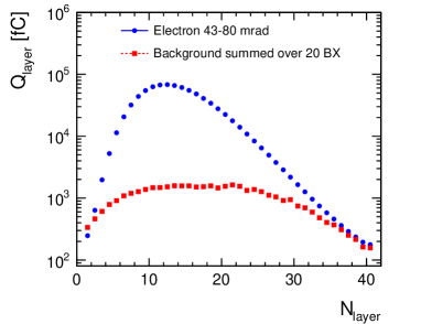
Figure 3: Comparison of the longitudinal profiles of energy deposition by EM showers and by the beam-induced background in the LumiCal at CLIC. Taken from ref. [24].

An adverse consequence of the rejection of events with high-energy electrons in the very forward region is that individual final-state particles from Bhabha events, detected in random coincidence with other processes, cause a loss of statistics because of indiscriminate rejection of a relatively large fraction of physics events. Taking into account the boost of the Bhabha event CM frame due to beam-beam effects, as well as the 0.5 ns bunch spacing at CLIC, and assuming a digitizer timing step of 10 ns, more than 30$\,\%$ of all events can be expected to be falsely tagged because of coincident detection of at least one final particle from a Bhabha event. In order to reduce the rate of coincident tagging of Bhabha particles, tagging was restricted to showers with energy higher than 200 GeV and polar angle above 1.7^∘ only. Under these conditions, the accidental tagging rate of Bhabha particles drops to 7$\,\%$. Table 2 summarises the rejection rates for the four-fermion and $\mathup{{{\mathup{{{e}}}}}^{\scriptstyle{\pm}}}\mathup{}\to\mathup{{{\mathup{{{e}}}}}^{\scriptstyle{\pm}}}\mathup{{}^{\scriptstyle{+}}}\mathup{{}^{\scriptstyle{-}}}$ processes, as well as for the signal. A large fraction of background with spectator electrons is removed in this way.

Process	Rejection rate by tagging final-state electrons	Total rejection including random Bhabha coincidence
$\mathup{{{\mathup{{{e}}}}}^{\scriptstyle{+}}}\mathup{{{\mathup{{{e}}}}}^{\scriptstyle{-}}}\to\mathup{{{\mathup{{{e}}}}}^{\scriptstyle{+}}}\mathup{{{\mathup{{{e}}}}}^{\scriptstyle{-}}}\mathup{{}^{\scriptstyle{+}}}\mathup{{}^{\scriptstyle{-}}}$	44$\,\%$	48$\,\%$
$\mathup{{{\mathup{{{e}}}}}^{\scriptstyle{\pm}}}\mathup{}\to\mathup{{{\mathup{{{e}}}}}^{\scriptstyle{\pm}}}\mathup{{}^{\scriptstyle{+}}}\mathup{{}^{\scriptstyle{-}}}$	38$\,\%$	42$\,\%$
Signal	0.2$\,\%$	7$\,\%$

Table 2: Rejection rates through EM shower tagging in the forward region for the most relevant signal and background processes.

6 Event selection

6.1 Preselection

In order to suppress the influence of the beam-induced background, only reconstructed particles with $p_{\text{T}}$ > 5 GeV were used in the analysis. Under this condition, the preselection of events was made by requiring a reconstruction of two muons in the event, with an invariant mass of the di-muon system in the range 105-145 GeV, as well as the absence of tagged electrons with energy above 200 GeV and polar angle above 1.7^∘.

6.2 MVA event selection

For the final selection, MVA techniques were used based on the Boosted Decision Tree (BDT) classifier implemented in the TMVA package. The following sensitive observables were used for the classification of events:

• Visible energy of the event excluding the energy of the di-muon system, $E_{vis}$,

• Transverse momentum of the di-muon system, $p_{\text{T}}(\mathup{}\mathup{})$,

• Scalar sum of the transverse momenta of the two selected muons, $p_{\text{T}}(\mathup{}_{1})+p_{\text{T}}(\mathup{}_{2})$,

• Boost of the di-muon system, $\beta=\left|p\right|/E$,

• Polar angle of the di-muon system, $\theta$,

• Cosine of the helicity angle, $\cos\theta^{*}=\frac{\vec{p^{\prime}}(\mathup{}_{1})\vec{p}(\mathup{}\mathup{})}{\left|p^{\prime}(\mathup{}_{1})\right|\left|p(\mathup{}\mathup{})\right|}$, where the apostrophe denotes the rest frame of the di-muon system.

Distributions of the sensitive observables for signal and all groups of background processes are given in the Appendix. The distributions of the process $\mathup{{{\mathup{{{e}}}}}^{\scriptstyle{+}}}\mathup{{{\mathup{{{e}}}}}^{\scriptstyle{-}}}\to\mathup{{{\mathup{}}}{}_{\scriptstyle{\!\mathup{{{e}}}}}}\mathup{{\overline{{\mathup{}}}}{}_{\scriptstyle{\!\mathup{{{e}}}}}}\mathup{{}^{\scriptstyle{+}}}\mathup{{}^{\scriptstyle{-}}}$ are very similar to those of the signal, implying that this process is irreducible by kinematic selections. The distributions of the process $\mathup{}\mathup{}\to\mathup{{{\mathup{}}}{}_{\scriptstyle{\!\mathup{}}}}\mathup{{\overline{{\mathup{}}}}{}_{\scriptstyle{\!\mathup{}}}}\mathup{{}^{\scriptstyle{+}}}\mathup{{}^{\scriptstyle{-}}}$ show small differences with respect to the signal. All processes with one or two spectator electrons show significant differences from the signal, primarily in the distribution of the visible energy. Further, for these processes the distribution of $p_{\text{T}}(\mathup{}\mathup{})$ exhibits a peak at low values of $p_{\text{T}}(\mathup{}\mathup{})$. This peak corresponds to events in which the di-muon system recoils against electron spectators or outgoing photons that are emitted below the angular cut of the very-forward EM-shower tagging.

The distribution of the BDT classifier variable for the signal and the main background processes is shown in Figure 4 (a). Clearly, the largest fraction of background events is very well separated from the signal, with the exception of $\mathup{}\mathup{}\to\mathup{{{\mathup{}}}{}_{\scriptstyle{\!\mathup{}}}}\mathup{{\overline{{\mathup{}}}}{}_{\scriptstyle{\!\mathup{}}}}\mathup{{}^{\scriptstyle{+}}}\mathup{{}^{\scriptstyle{-}}}$ and $\mathup{{{\mathup{{{e}}}}}^{\scriptstyle{\pm}}}\mathup{}\to\mathup{{{\mathup{{{e}}}}}^{\scriptstyle{\pm}}}\mathup{{{\mathup{}}}{}_{\scriptstyle{\!\mathup{}}}}\mathup{{\overline{{\mathup{}}}}{}_{\scriptstyle{\!\mathup{}}}}\mathup{{}^{\scriptstyle{+}}}\mathup{{}^{\scriptstyle{-}}}$ events that are separated to some extent, and the irreducible process $\mathup{{{\mathup{{{e}}}}}^{\scriptstyle{+}}}\mathup{{{\mathup{{{e}}}}}^{\scriptstyle{-}}}\to\mathup{{{\mathup{}}}{}_{\scriptstyle{\!\mathup{{{e}}}}}}\mathup{{\overline{{\mathup{}}}}{}_{\scriptstyle{\!\mathup{{{e}}}}}}\mathup{{}^{\scriptstyle{+}}}\mathup{{}^{\scriptstyle{-}}}$ that shows almost the same distribution as the signal. The classifier cut position was selected to maximise the significance, defined as $N_{s}/\sqrt{N_{s}+N_{b}}$, where $N_{s}$ and $N_{b}$ are the number of selected signal and background events, respectively. A plot of significance as a function of the position of the BDT cut is shown in Figure 4 (b). The optimal cut position was found at BDT = 0.098.

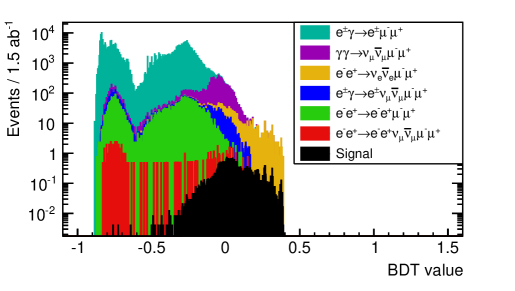
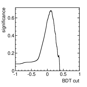
(a)                                                           (b)

Figure 4: Stacked histograms of the BDT classifier distribution for the signal and the background processes (a) and the significance as a function of the BDT cut position (b).

Distributions of the di-muon invariant mass are shown in Figure 5. Figure 5 (a) includes all events that pass the preselection, while Figure 5 (b) shows all events passing the BDT selection, as well. All samples were normalised to an integrated luminosity of $1.5\,\text{ab}^{-1}$. The MVA selection efficiency for the signal is 32$\,\%$. The overall signal efficiency including reconstruction, preselection, losses due to coincident tagging of Bhabha particles and the MVA is 26$\,\%$, resulting in an expected number of 20 signal events.

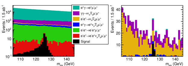
(a)                                                                        (b)

Figure 5: Stacked histograms of the Di-muon invariant mass distributions with preselecton only (a) and after BDT selection (b).

7 Di-muon invariant mass fit

The key observable for the determination of $\sigma(\mathup{{{H}}}\mathup{}\mathup{})\times\text{BR}(\mathup{{{H}}}\to\mathup{{}^{\scriptstyle{+}}}\mathup{{}^{\scriptstyle{-}}})$ is the number of selected signal events $N_{s}$ passing the final selection.

$$\sigma(\mathup{{{H}}}\mathup{}\mathup{})\times\text{BR}(\mathup{{{H}}}\to\mathup{{}^{\scriptstyle{+}}}\mathup{{}^{\scriptstyle{-}}})=\frac{N_{s}}{L\cdot\epsilon_{s}}$$ (1)

where $L$ is the integral luminosity given in units of $\,\mathrm{fb}^{-1}$ and $\epsilon_{s}$ is the total counting efficiency for the signal, including the reconstruction, preselection and MVA selection efficiencies.

In the experiment, the number of signal events is determined by fitting the model of the combined Probability Density Function (PDF), $f(m)$, of the di-muon invariant mass, $m$, for the signal and the background to the measured $m$ distribution,

$$f(m)=N_{s}f_{s}(m)+N_{b}f_{b}(m)$$ (2)

where $f_{s}(m)$ and $f_{b}(m)$ are the PDF for the signal and the background, respectively, and $N_{s}$ and $N_{b}$ are the respective numbers of signal and background events in the fitting window. The extraction of $f_{s}(m)$ and $f_{b}(m)$ from simulated data is described in Section 7.1.

In order to estimate the statistical uncertainty of the present analysis, 5000 Toy Monte-Carlo (MC) experiments were performed where pseudo-data were obtained by randomly picking signal $m$ values from the fully simulated signal sample, while background $m$ values were randomly generated from the background PDF. The sample sizes, $N_{s}$ and $N_{b}$, were sampled in each Toy MC experiment from the Poisson distribution with the respective mean values $\left<N_{s/b}\right>=L\cdot\sigma_{s/b}\cdot\epsilon_{s/b}$, where the integral luminosity $L$ is $1.5\;\text{ab}^{-1}$, $\epsilon_{s/b}$ is the total selection efficiency, and $\sigma_{s/b}$ the corresponding cross-section for the signal and the background, respectively. For each Toy MC experiment, the $m$ distribution is fitted by the function (2), and the RMS of the resulting distribution of $N_{s}$ over all Toy MC experiments is taken as the estimate of the statistical uncertainty of the measurement.

7.1 Signal and background PDF

The signal and background PDF were extracted by fitting to fully simulated datasets after the preselection and the MVA selection.

The signal sample was fitted with an ad-hoc function composed of a Gaussian with a flat tail and a Gaussian with an exponential tail (Eq. (5), Figure 6). The likelihood fit was performed with unbinned data using RooFit [25]. The results of the fit are listed in Table 3.

$$f_{s} =f_{flat}+C\cdot f_{exp}$$

$$f_{flat} =\left\{\begin{array}[]{rl}e^{-\frac{(m-m_{\mathup{{{H}}}})^{2}}{2\sigma^{2}+\beta_{L}(m-m_{\mathup{{{H}}}})^{2}}}&m<m_{\mathup{{{H}}}}\\ e^{-\frac{(m-m_{\mathup{{{H}}}})^{2}}{2\sigma^{2}+\beta_{R}(m-m_{\mathup{{{H}}}})^{2}}}&m>m_{\mathup{{{H}}}}\end{array}\right.$$ (5)

$$f_{exp} =\left\{\begin{array}[]{rl}e^{-\frac{(m-m_{\mathup{{{H}}}})^{2}}{2\sigma^{2}+\alpha_{L}|m-m_{\mathup{{{H}}}}|}}&m<m_{\mathup{{{H}}}}\\ e^{-\frac{(m-m_{\mathup{{{H}}}})^{2}}{2\sigma^{2}+\alpha_{R}|m-m_{\mathup{{{H}}}}|}}&m>m_{\mathup{{{H}}}}\end{array}\right.$$ (8)

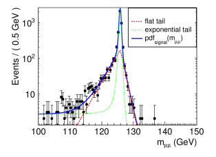
Figure 6: Distribution of the invariant mass, $m$, in the signal sample after MVA selection, and the corresponding fit to the data. The fit was performed in the range corresponding to the preselection cut in the analysis. The extension of the line below 105$\,\mathrm{GeV}$ is a graphical extrapolation.

Parameter	fitted value
$C$	$0.076\pm 0.008$
$\alpha_{L}$	$2.49\pm 0.19\,\mathrm{GeV}$
$\alpha_{R}$	$0.94\pm 0.06\,\mathrm{GeV}$
$\beta_{L}$	$0.157\pm 0.004$
$\beta_{R}$	$0.126\pm 0.006$
$m_{\mathup{{{H}}}}$	$125.847\pm 0.006\,\mathrm{GeV}$
$\sigma$	$0.246\pm 0.007\,\mathrm{GeV}$

Table 3: Fitted parameters of the distribution of the invariant mass, $m$, of the signal.

The $m$ distribution from the inclusive background data sample after event selection was fitted with a linear combination of a constant and an exponential term,

$$f_{b}=p_{0}(p_{1}e^{p_{2}(m-m_{\mathup{{{H}}}})}+(1-p_{1}))$$ (9)

The fit results for background are shown in Figure 7. As the normalisation to the common integrated luminosity requires different normalisation coefficients for different processes, binned data were used to combine the background processes in a straightforward manner, and binned $\chi^{2}$ fit was performed. The $\chi^{2}/N_{df}$ of the background fit was 62/61.

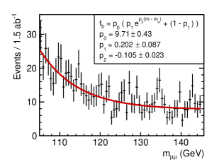
Figure 7: Distribution of the invariant mass, $m$, for the sum of all background processes after event selection. The result of the fit is also shown.

The overall function $f(m)$ (2) was fitted to the pseudo data of each Toy MC “experiment” using the unbinned likelihood method, and fixing all parameters of $f(m)$ except $N_{s}$ and $N_{b}$. An example of a Toy MC fit is given in Figure 8.

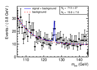
Figure 8: Distribution of the invariant mass, $m$, for the sum of the signal and background samples in one Toy MC run, together with the fit of the combined PDF model (Eq. (2)).

7.2 Distribution of the signal count

The RMS deviation of the resulting signal count distribution in 5000 repeated Toy MC experiments corresponds to the statistical uncertainty of the measurement (Figure 9 (a)). The pull distribution (Figure 9 (b)) is approximately centered at 0 and has an approximate width of 1, confirming that the PDFs of the signal and background di-muon invariant mass are adequate.

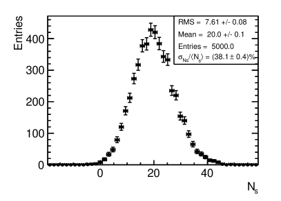
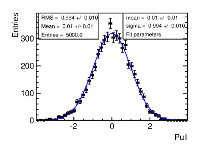
(a)                                                              (b)

Figure 9: Distribution of the number of signal events in the Toy MC experiments (a); the corresponding Pull distribution (b)

The relative statistical uncertainty of $\sigma(\mathup{{{H}}}\mathup{}\mathup{})\times\text{BR}(\mathup{{{H}}}\to\mathup{{}^{\scriptstyle{+}}}\mathup{{}^{\scriptstyle{-}}})$ is 38$\,\%$. This uncertainty is dominated by the contributions from the limited signal statistics and from the presence of irreducible backgrounds in the $\mathup{{{H}}}\to\mathup{{}^{\scriptstyle{+}}}\mathup{{}^{\scriptstyle{-}}}$ measurement. With 80$\,\%$ left-handed polarisation of the electron beam and 30$\,\%$ right handed polarisation for the positrons during the entire operation time at 1.4$\,\mathrm{TeV}$, the Higgs production through $\mathup{{{W}}}\mathup{{{W}}}$ fusion would be enhanced by a factor 2.34 [4]. The most important background contribution after the MVA selection, the $\mathup{{{\mathup{{{e}}}}}^{\scriptstyle{+}}}\mathup{{{\mathup{{{e}}}}}^{\scriptstyle{-}}}\to\mathup{{{\mathup{}}}{}_{\scriptstyle{\!\mathup{{{e}}}}}}\mathup{{\overline{{\mathup{}}}}{}_{\scriptstyle{\!\mathup{{{e}}}}}}\mathup{{}^{\scriptstyle{+}}}\mathup{{}^{\scriptstyle{-}}}$ process, is enhanced by the same factor because it is also mediated by $\mathup{{{W}}}$ bosons, which have only left-handed interactions. The remaining background processes are enhanced by a smaller factor, or not enhanced at all. In the conservative estimate, the statistical uncertainty is improved by a factor $1/\sqrt{2.34}$, neglecting the differences in the production ratio for the background processes, as well as the increase in the MVA selection efficiency for the signal due to the change in the optimal BDT cut. The upper limit of the statistical uncertainty with polarized beams is thus 25$\,\%$. As the polarization in principle affects the distributions of the kinematical observables, a precise estimate is possible only with the full simulation with polarized beams.

To estimate the significance of the signal against the null-hypothesis, another set of 5000 Toy MC runs was performed with zero signal count, and $f(m_{\mu\mu})$ (2) was fitted to the pseudo data. The resulting $N_{s}$ distribution was centered on zero with the standard deviation $\sigma_{N_{s}}(H_{0})=5.4$. Thus, in case the SM expected number of events $N_{s,SM}=20$ is realized in the experiment, the signal significance would be $3.7\,\upsigma$.

The Higgs coupling to muons, $g_{\mathup{{{H}}}\mathup{}\mathup{}}$, is optimally extracted in a global fit procedure taking into account all Higgs measurements both at the 350$\,\mathrm{GeV}$ and 1.4$\,\mathrm{TeV}$ stages, and extracting all involved Higgs couplings, as well as the total Higgs width in the same procedure. However, even in the suboptimal procedure of extraction of $g_{\mathup{{{H}}}\mathup{}\mathup{}}$ involving the present measurement alongside measurements giving access to $\Gamma_{\mathup{{{H}}}}$ and $g_{\mathup{{{H}}}\mathup{{{W}}}\mathup{{{W}}}}$, the dominant contribution to the coupling uncertainty is the statistical uncertainty of the $\mathup{{{H}}}\to\mathup{{}^{\scriptstyle{+}}}\mathup{{}^{\scriptstyle{-}}}$ measurement. An example of a minimal set of measurements giving model-independent access to $\Gamma_{\mathup{{{H}}}}$ and $g_{\mathup{{{H}}}\mathup{{{W}}}\mathup{{{W}}}}$ is the following: the recoil mass measurement at 350$\,\mathrm{GeV}$ giving access to $g_{\mathup{{{H}}}\mathup{{{Z}}}\mathup{{{Z}}}}$, the $\mathup{{{H}}}\to\mathup{{{b}}}\mathup{{\overline{{\mathup{{{b}}}}}}}$ measurements at both 350$\,\mathrm{GeV}$ and 1.4$\,\mathrm{TeV}$ stages giving access to the ratio $g_{\mathup{{{H}}}\mathup{{{W}}}\mathup{{{W}}}}$/$g_{\mathup{{{H}}}\mathup{{{Z}}}\mathup{{{Z}}}}$ and the $\mathup{{{H}}}\to\mathup{{{\mathup{{{W}}}}}^{\scriptstyle{+}}}\mathup{{{\mathup{{{W}}}}}^{\scriptstyle{-}}}$ measurement at 1.4$\,\mathrm{TeV}$ giving access to the ratio $g_{\mathup{{{H}}}\mathup{{{W}}}\mathup{{{W}}}}^{4}/\Gamma_{\mathup{{{H}}}}$ [4]. Assuming that no correlations exist between uncertainties of these measurements, their relative uncertainties add up quadratically to form the relative uncertainty of $g_{\mathup{{{H}}}\mathup{}\mathup{}}^{2}$. However, the contributions of measurement uncertainties other than the statistical uncertainty of the $\sigma(\mathup{{{H}}}\mathup{}\mathup{})\times\text{BR}(\mathup{{{H}}}\to\mathup{{}^{\scriptstyle{+}}}\mathup{{}^{\scriptstyle{-}}})$ measurement affect the final uncertainty only at the third significant digit, and can be neglected. Thus, the relative uncertainty of $g_{\mathup{{{H}}}\mathup{}\mathup{}}$ is 19$\,\%$. A summary of the results of the present analysis is given in Table 4.

$N_{s}$	$20.0\pm 7.6$
$\epsilon_{s}$	26$\,\%$
$\frac{\delta(\sigma(\mathup{{{H}}}\mathup{}\mathup{})\times\text{BR}(\mathup{{{H}}}\to\mathup{{}^{\scriptstyle{+}}}\mathup{{}^{\scriptstyle{-}}}))}{\sigma(\mathup{{{H}}}\mathup{}\mathup{})\times\text{BR}(\mathup{{{H}}}\to\mathup{{}^{\scriptstyle{+}}}\mathup{{}^{\scriptstyle{-}}})}$	38$\,\%$
$\delta(g_{\mathup{{{H}}}\mathup{}\mathup{}})/g_{\mathup{{{H}}}\mathup{}\mathup{}}$	19$\,\%$

Table 4: Summary of the results of the analysis of the $\sigma(\mathup{{{H}}}\mathup{}\mathup{})\times\text{BR}(\mathup{{{H}}}\to\mathup{{}^{\scriptstyle{+}}}\mathup{{}^{\scriptstyle{-}}})$ measurement at 1.4 TeV CLIC with unpolarised beams. All uncertainties are statistical.

8 Benefit of a better $p_{\text{T}}$ resolution

To estimate the eventual benefit of a better $p_{\text{T}}$ resolution, the analysis was repeated with substitution of the muon four-momenta reconstructed in the full simulation in the signal sample by the four-momenta obtained by a parametrisation of the momentum resolution ("fast simulation") for several different values of the resolution. Figure 10 displays the approximate dependence of the statistical uncertainty of the measurement on the average transverse momentum resolution in the whole detector. It is clear that even a large improvement of the momentum resolution would result in only a moderate improvement of the statistical uncertainty of the measured product of the cross-section and the branching ratio.

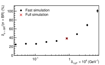
Figure 10: Dependence of the relative statistical uncertainty of the $\sigma(\mathup{{{H}}}\mathup{}\mathup{})\times\text{BR}(\mathup{{{H}}}\to\mathup{{}^{\scriptstyle{+}}}\mathup{{}^{\scriptstyle{-}}})$ on the transverse momentum resolution, $\delta_{1/p_{\text{T}}}$, averaged over the signal sample in the whole detector.

9 Systematic uncertainties

From Eq. (1) it is clear that uncertainties of the integral luminosity and muon identification efficiency influence the uncertainty of the branching ratio measurement at the systematic level. It has been shown in [26] that at a 3 TeV CLIC, where the impact of the beam-induced processes is the most severe, luminosity above ca. 75$\,\%$ of the nominal CM energy can be determined at the permille level using low-angle Bhabha scattering. Below 75$\,\%$ of the nominal CM energy the luminosity spectrum can be measured with a precision of a few percent using wide-angle Bhabha scattering [27]. About 17$\,\%$ of all Higgs events occur at a CM energy of the initial $\mathup{{{\mathup{{{e}}}}}^{\scriptstyle{+}}}\mathup{{{\mathup{{{e}}}}}^{\scriptstyle{-}}}$ pair below 75$\,\%$ of the nominal CM energy. Having in mind the intrinsic statistical limitations of the signal sample, this source of systematic uncertainty can be considered negligible.

On the detector side, an important systematic effect is the uncertainty on the transverse momentum resolution, because it directly influences the expected shape of the signal $m$ distribution. The sensitivity of the signal count to the accuracy of the knowledge of the $p_{\text{T}}$ resolution has been studied by performing the analysis with an artificially introduced error of an exaggerated magnitude on the assumed $p_{\text{T}}$ resolution used to extract the signal $m$ PDF. Results are shown in Figure 11. The relative counting bias $\,\mathrm{d}N_{s}/N_{s}$ per one percent bias of $\sigma_{pT}$ is 0.35$\,\%$.

The uncertainty of the muon identification efficiency will directly influence the signal selection efficiency. In addition, the uncertainty of the muon polar angle resolution impacts the $m$ reconstruction. Based on the results of the LEP experiments [28], it can be assumed that these detector related uncertainties are below a percent.

Because of the forward EM shower tagging, about 7$\,\%$ of signal events are rejected by coincidence with the detection of at least one of the final Bhabha particles. This fraction must be precisely calculated taking into account Bhabha event distributions, beam-beam effects, as well as the dependence of the tagging efficiency on energy and angle of incident electrons and photons. This is work in progress [29, 30, 31], but the uncertainty of this effect is also expected to be negligible compared to the statistical uncertainty of this measurement.

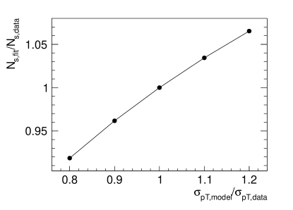
Figure 11: Impact of the uncertainty of the muon $p_{\text{T}}$ resolution on signal counting. The relative shift of the signal count is given as a function of the relative shift of the $p_{\text{T}}$ resolution.

10 Conclusions

There is a strong motivation to use precise Higgs measurements at CLIC to search for physics beyond the Standard Model. The measurement of Higgs boson couplings are of particular interest. The measurement of the branching ratio for the rare SM-like Higgs decay into two muons was simulated at a 1.4 CLIC collider with unpolarised beams. The measurement itself tests the muon identification and momentum resolution of the detector.

It was shown that the measurement of the cross-section times the branching ratio for the Standard Model Higgs decay into two muons can be performed with a statistical uncertainty of 38$\,\%$, assuming 1.5 $\text{ab}^{-1}$ integrated luminosity with unpolarized beams. If the same integrated luminosity is collected with 80$\,\%$ left-handed polarisation for the electrons and 30$\,\%$ right handed polarisation for the positrons, the statistical uncertainty improves to beter than 25%. The systematic uncertainties are negligible in comparison. The largest contributions to the statistical uncertainty come from the limited statistics of the signal and from the presence of the signal-like backgrounds from $\mathup{{{\mathup{{{e}}}}}^{\scriptstyle{+}}}\mathup{{{\mathup{{{e}}}}}^{\scriptstyle{-}}}\to\mathup{{{\mathup{}}}{}_{\scriptstyle{\!\mathup{{{e}}}}}}\mathup{{\overline{{\mathup{}}}}{}_{\scriptstyle{\!\mathup{{{e}}}}}}\mathup{{}^{\scriptstyle{+}}}\mathup{{}^{\scriptstyle{-}}}$ and $\mathup{}\mathup{}\to\mathup{{{\mathup{}}}{}_{\scriptstyle{\!\mathup{}}}}\mathup{{\overline{{\mathup{}}}}{}_{\scriptstyle{\!\mathup{}}}}\mathup{{}^{\scriptstyle{+}}}\mathup{{}^{\scriptstyle{-}}}$ processes. The uncertainty of $\sigma(\mathup{{{H}}}\mathup{}\mathup{})\times\text{BR}(\mathup{{{H}}}\to\mathup{{}^{\scriptstyle{+}}}\mathup{{}^{\scriptstyle{-}}})$ of 38$\,\%$ translates into the uncertainty of Higgs coupling to muons, $g_{\mathup{{{H}}}\mathup{}\mathup{}}$, of 19$\,\%$.

Appendix

Figures 12 and 13 show the distributions, before and after the MVA selection, respectively, of the sensitive variables used in the MVA analysis to separate the signal from the background.

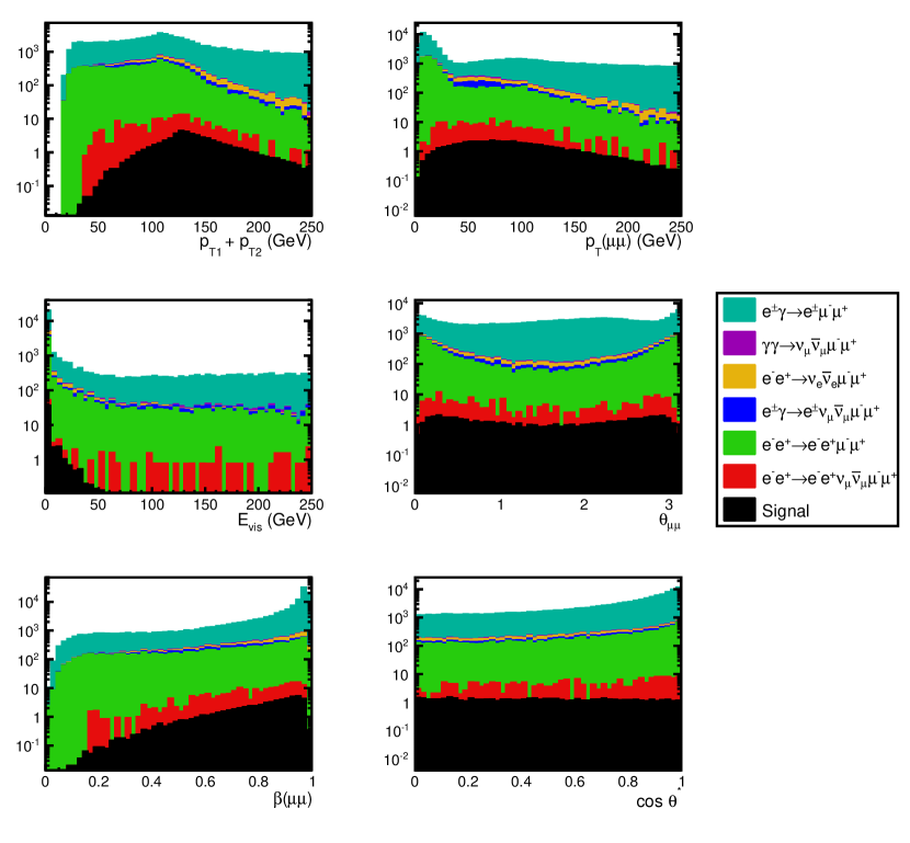
Figure 12: Distributions of the sensitive variables used in the MVA analysis for events that pass the preselection cuts.

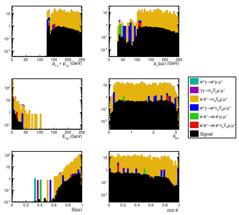
Figure 13: Distributions of the sensitive variables used in the MVA analysis for events that pass the preselection and the MVA selection.

References

- [1] Rick S. Gupta, Heidi Rzehak and James D. Wells “How well do we need to measure Higgs boson couplings?” arXiv:1206.3560 In Phys. Rev. D 86 American Physical Society, 2012 DOI: 10.1103/PhysRevD.86.095001
- [2] C. Englert et al. “Precision Measurements of Higgs Couplings: Implications for New Physics Scales” arXiv:1403.7191 In J. Phys G, 2014
- [3] “Physics and Detectors at CLIC: CLIC Conceptual Design Report” ANL-HEP-TR-12-01, CERN-2012-003, DESY 12-008, KEK Report 2011-7, arXiv:1202.5940 CERN, 2012
- [4] H. Abramowicz “Physics at the CLIC Linear Collider – Input to the Snowmass process 2013” arXiv:1307.5288, 2013
- [5] S. Dittmaier, C. Mariotti, G. Passarino and R. Tanaka “Handbook of LHC Higgs Cross Sections: 2. Differential Distributions” arXiv:1201.3084, 2012
- [6] The ATLAS Collaboration “Search for the Standard Model Higgs boson decay to with the ATLAS detector” arXiv:1406.7663, CERN-PH-EP-2014-131, 2014
- [7] Justin Hugon for the CMS Collaboration “Search for the Standard Model Higgs boson decaying to in pp collisions at = 7 and 8 TeV” arXiv:1409.0839, CMS-CR-2014-189, 2014
- [8] The ATLAS Collaboration “Projections for measurements of Higgs boson cross sections, branching ratios and coupling parameters with the ATLAS detector at a HL-LHC” ATL-PHYS-PUB-2013-014
- [9] “The CLIC Programme: towards a staged Linear Collider exploring the Terascale” ANL-HEP-TR-12-51, CERN-2012-005, KEK Report 2012-2, MPP-2012-115, CERN, 2012
- [10] C. Grefe “Light Higgs decay into muons in the CLIC_SiD CDR detector” CERN LCD-Note-2011-035, 2011
- [11] A. Münnich and A. Sailer “The CLIC_ILD_CDR Geometry for the CDR Monte Carlo Mass Production” LCD-Note-2011-002 , LCD-Note, 2011
- [12] Wolfgang Kilian, Thorsten Ohl and Jurgen Reuter “WHIZARD: Simulating Multi-Particle Processes at LHC and ILC” arXiv:0708.4233 In Eur. Phys. J. C71, 2011 DOI: 10.1140/epjc/s10052-011-1742-y
- [13] T. Sjostrand, S. Mrenna and P. Z. Skands “PYTHIA 6.4 Physics and Manual” arXiv:hep-ph/0603175 In JHEP 05, 2006 DOI: 10.1088/1126-6708/2006/05/026
- [14] D. Schulte “Beam-beam simulations with GUINEA-PIG” CERN-PS-99-014-LP, 1999
- [15] P. Freitas and H. Videau “Detector Simulation with Mokka/Geant4 : Present and Future” LC-TOOL-2003-010 In International Workshop on Linear Colliders (LCWS 2002), 2002
- [16] S. Agostinelli “Geant4 – A Simulation Toolkit” In Nucl. Instrum. Methods Phys. Res., Sect. A 506.3, 2003
- [17] M. A. Thomson “Particle Flow Calorimetry and the PandoraPFA Algorithm” arXiv:0907.3577 In Nucl. Instrum. Methods A611, 2009 DOI: 10.1016/j.nima.2009.09.009
- [18] J.S. Marshall, A. Münnich and M.A. Thomson “Performance of Particle Flow Calorimetry at CLIC” arXiv:1209.4039 In Nucl. Instrum. Methods A700, 2013 DOI: 10.1016/j.nima.2012.10.038
- [19] O. Wendt, F. Gaede and T. Kramer “Event reconstruction with MarlinReco at the ILC” arXiv:physics/0702171 In Pramana 69, 2007 DOI: 10.1007/s12043-007-0237-8
- [20] A. Höcker et al. “TMVA - Toolkit for multivariate data analysis” arXiv:physics/0703039, 2009
- [21] T. Abe “The International Large Detector: Letter of Intent” arXiv:1006.3396, 2010
- [22] H. Abramowicz “Forward instrumentation for ILC detectors” arXiv:1009.2433 In JINST 5, 2010 DOI: 10.1088/1748-0221/5/12/P12002
- [23] D. Dannheim and A. Sailer “Beam-induced Backgrounds in the CLIC Detectors”, LCD-Note, LCD-Note-2011-021, 2011
- [24] Rina Schwartz “Luminosity measurement at the Compact Linear Collider” CERN-THESIS-2012-345, MSc thesis, Tel Aviv University, Tel Aviv, Israel, 2012
- [25] W. Verkerke and D. P. Kirkby “The RooFit toolkit for data modeling” arXiv:physics/0306116, 2003
- [26] S Lukić, I Božović-Jelisavčić, M Pandurović and I Smiljanić “Correction of beam-beam effects in luminosity measurement in the forward region at CLIC” LCD-Note-2012-008, arXiv:1301.1449 In JINST 8, 2013
- [27] Stéphane Poss and André Sailer “Luminosity spectrum reconstruction at linear colliders” In Eur. Phys. J C74 Springer Berlin Heidelberg, 2014 DOI: 10.1140/epjc/s10052-014-2833-3
- [28] M. Grünewald and others “Precision electroweak measurements on the resonance” arXiv:hep-ex/0509008 In Phys. Rep. 427, 2006 DOI: 10.1016/j.physrep.2005.12.006
- [29] V. Makarenko “Status of new generator for Bhabha scattering” presented at the CLIC workshop, CERN, 2014 URL: https://indico.cern.ch/event/275412/session/5/contribution/183/material/slides/0.pdf
- [30] A. Sailer “Status Report on Forward Region Studies at CLIC” presented at the CLIC workshop, CERN, 2014 URL: https://indico.cern.ch/event/275412/session/5/contribution/171/material/slides/0.pdf
- [31] Strahinja Lukić “Forward electron tagging at ILC/CLIC” presented at the CLIC workshop, CERN, 2014 URL: https://indico.cern.ch/event/275412/session/5/contribution/172/material/slides/0.pdf