Time correlation functions for non-Hermitian quantum systems

Abstract

We introduce a formalism for time-dependent correlation functions for systems whose evolutions are governed by non-Hermitian Hamiltonians of general type. It turns out that one can define two different types of time correlation functions. Both these definitions seem to be physically consistent while becoming equivalent only in certain cases. Moreover, when autocorrelation functions are considered, one can introduce another function defined as the relative difference between the two definitions. We conjecture that such a function can be used to assess the positive semi-definiteness of the density operator without computing its eigenvalues. We illustrate these points by studying analytically a number of models with two energy levels.

I Introduction

Quantum dynamics of systems governed by non-Hermitian (NH) Hamiltonians is currently a very popular field of research. For example, this includes areas such as quantum transport and scattering by complex potentials suu54 ; ck58 ; lay63 ; bender07 ; varga ; berg ; miro ; varga2 ; muga ; thila , resonances and decaying states nimrod2 ; seba ; spyros ; fesh ; sudarshan , multiphoton ionization selsto ; baker ; baker2 ; chu , optical waveguides optics ; optics2 , and the theory of open quantum systems kor64 ; wong67 ; heg93 ; bas93 ; ang95 ; rotter ; rotter2 ; gsz08 ; bellomo ; banerjee ; reiter ; sz13 ; bg12 ; sz14 . Notwithstanding the long history, the core of the formalism of non-Hermitian quantum dynamics is still a topic of active research ghk10 ; ale ; grsc11 ; sz13 ; bg12 ; sz14 . From the viewpoint of the general formalism, one can divide the whole field of research into two main branches: pseudo-Hermitian quantum dynamics (together with the synonymous or sister theories, such as quasi-Hermitian and ${\cal PT}$-symmetric quantum mechanics) sgh92 ; ben99 ; zno02 ; mos10 and general non-Hermitian formalism. The former branch deals mainly with a class of NH Hamiltonians that have purely real eigenvalues. The latter branch, to which the study reported in this paper belongs, attempts to find a way to adopt general NH Hamiltonians as an effective tool for the description of dissipative processes. As regards this goal, the real-valuedness of the spectrum of the Hamiltonian operator is not compulsory - on the contrary, in some cases, it would be too restrictive. Indeed, the real parts of the eigenvalues can be related to the energy, as usual, whereas the imaginary parts can be linked to decay rates.

In this paper, we continue along the line of research started in Ref. sz13 . Our aim is to build a consistent formalism of quantum statistical mechanics when the dynamics is generated by non-Hermitian Hamiltonians. In Ref. sz13 , we adopted a well-defined quantum evolution equation for the density operator and considered a definition of statistical averages that allows one to retain the probabilistic interpretation of the density matrix. Here, our interest is devoted to the definition and study of the multi-time correlation functions since they are often directly related to measurable quantities, such as structure factors, fluctuation spectra, and scattering rates gzbook ; bpbook .

This paper is structured as follows. In Sec. II we give a brief outline of the quantum non-Hermitian approach. In Sec. III.1 we sketch the formalism for multi-time correlation functions in the conventional (Hermitian) case. In Sec. III.2 we generalize the formalism for multi-time correlation functions to the case of quantum dynamics generated by non-Hermitian Hamiltonians. In Sec. IV we apply such a formalism to a specific example: we compute the two-point correlation functions for a number of two-level systems (TLSs), which were also considered in sz13 . A summary is given in Sec. V.

II Non-Hermitian dynamics and averages

Let us consider a non-Hermitian Hamiltonian $\hat{H}\neq\hat{H}^{{\dagger}}$, which can be always written in the form

$$\hat{H}=\hat{H}_{+}-i\hat{\Gamma},$$ (1)

where $\hat{H}_{+}=\hat{H}_{+}^{{\dagger}}$ and $\hat{\Gamma}=\hat{\Gamma}^{{\dagger}}$. It can be shown that the evolution equation for the non-normalized density matrix $\hat{\Omega}$ can be written as

$$\frac{d}{dt}\hat{\Omega}(t) = -\frac{i}{\hbar}\left[\hat{H}_{+},\hat{\Omega}(t)\right]-\frac{1}{\hbar}\left\{\hat{\Gamma},\hat{\Omega}(t)\right\},$$ (2)

where the square brackets on the right hand side of Eq. (2) denote the commutator while the curly brackets denote the anti-commutator. In the context of theory of open quantum systems the evolution equation for the density operator $\hat{\Omega}$ effectively describes the original subsystem (with Hamiltonian $\hat{H}_{+}$) together with the effect of environment (represented by $\hat{\Gamma}$). Upon taking the trace of Eq. (2) one obtains:

$$\frac{d}{dt}{\rm tr}\hat{\Omega}(t) = -\frac{2}{\hbar}{\rm tr}\left(\hat{\Omega}(t)\hat{\Gamma}\right),$$ (3)

which shows that the trace of $\hat{\Omega}$ is not conserved during the evolution governed by a NH Hamiltonian. Defining the normalized density matrix as

$$\hat{\rho}(t)=\frac{\hat{\Omega}(t)}{{\rm tr}\hat{\Omega}(t)},$$ (4)

and using Eq. (3) we can obtain a non-linear equation of motion for $\hat{\rho}(t)$

$$\frac{d}{dt}\hat{\rho}(t)=-\frac{i}{\hbar}\left[\hat{H}_{+},\hat{\rho}(t)\right]-\frac{1}{\hbar}\left\{\hat{\Gamma},\hat{\rho}(t)\right\}+\frac{2}{\hbar}\hat{\rho}(t){\rm tr}\left(\hat{\rho}(t)\hat{\Gamma}\right),$$ (5)

which can be brought back into a linear form by using (4) as an ansatz (provided the initial condition $\text{tr}\hat{\rho}(t_{0})=1$ is assumed). The evolution equation for the normalized density operator effectively describes the original subsystem (with Hamiltonian $\hat{H}_{+}$) together with the effect of environment (represented by $\hat{\Gamma}$) and the additional term that restores the overall probability’s conservation. For the detailed discussion of important features of time evolution driven by NH Hamiltonians, such as the purity’s non-conservation and independence from the absolute value of the energy, the reader is referred to Refs. sz13 ; sz14 .

Given an arbitrary operator $\hat{\chi}$, its statistical average can be defined as

$$\langle\hat{\chi}(t)\rangle\equiv{\rm tr}\left(\hat{\rho}(t)\hat{\chi}\right)=\frac{{\rm tr}\left(\hat{\Omega}(t)\hat{\chi}\right)}{{\rm tr}\hat{\Omega}(t)},$$ (6)

which reduces to the standard quantum statistical rule in the case of Hermitian Hamiltonians.

III Time correlation functions

In the following we sketch the formalism for the two-time correlation functions in the Hermitian case in Sec. III.1. Its generalization to the non-Hermitian case is given in Sec. III.2.

III.1 Hermitian case

Given two arbitrary operators $\hat{\chi}$ and $\hat{\xi}$, it is known that their time-dependent correlation function in the Heisenberg picture of Hermitian quantum mechanics is defined as

$$C_{\chi\xi}(t_{2},t_{1})\equiv\langle\hat{\chi}(t_{2})\hat{\xi}(t_{1})\rangle\equiv{\rm tr}\left(\hat{\chi}(t_{2})\hat{\xi}(t_{1})\hat{\rho}(0)\right).$$ (7)

Now, assuming that the evolution takes place under the Hermitian operator $\hat{H}_{+}$, upon using the definition of the time-dependent Heisenberg operator ($\hat{\chi}(t)\equiv\exp\left[\frac{it}{\hbar}\hat{H}_{+}\right]\hat{\chi}\exp\left[\frac{-it}{\hbar}\hat{H}_{+}\right]$), and the properties of the trace, the Hermitian correlation function (7) can be rewritten as

$$C_{\chi\xi}(t_{2},t_{1})={\rm tr}\left\{\hat{\chi}\exp\left[\frac{-i(t_{2}-t_{1})}{\hbar}\hat{H}_{+}\right]\hat{\xi}\hat{\rho}_{\hat{H}_{+}}(t_{1})\exp\left[\frac{i(t_{2}-t_{1})}{\hbar}\hat{H}_{+}\right]\right\},$$ (8)

where

$$\hat{\rho}_{\hat{H}_{+}}(t_{1})\equiv\exp\left[\frac{-it_{1}}{\hbar}\hat{H}_{+}\right]\hat{\rho}\exp\left[\frac{it_{1}}{\hbar}\hat{H}_{+}\right].$$ (9)

The definition given in Eq. (8) represents the correlation function written in the Schrödinger picture, where the time dependence has been transferred from the operators to the density matrix. We take the Schrödinger form of the correlation function as the basis for the generalization to the non-Hermitian case, which is treated in Sec. III.2.

III.2 Non-Hermitian case

When the Hermitian Hamiltonian $\hat{H}_{+}$ is augmented by a non-Hermitian part $\hat{H}_{-}=-i\Gamma$, a natural generalization of Eq. (8) is

$${\cal C}_{\xi\chi}(t_{1},t_{2}) = {\rm tr}\left\{\hat{\chi}{\cal K}(t_{2},t_{1})\hat{\xi}{\cal K}(t_{1},t_{0})\hat{\rho}(t_{0})\right\}$$ (10)

$$= {\rm tr}\left\{\hat{\chi}{\cal K}(t_{2},t_{1})\hat{\xi}\hat{\rho}(t_{1})\right\}$$

$$= {\rm tr}\left\{\hat{\chi}{\cal K}(t_{2},t_{1})\{\hat{\xi}\hat{\Omega}(t_{1})/{\rm tr}\hat{\Omega}(t_{1})\}\right\},$$

where $\hat{\chi}$ and $\hat{\xi}$ are operators in the Schrödinger presentation, and ${\cal K}$ is the (generalized) evolution operator defined as follows. When ${\cal K}(t_{b},t_{a})$ is applied to anything on its right, it evolves it from time $t_{a}$ up to time $t_{b}$ using Eq. (5). Hence, in the expression above, the first application of ${\cal K}$ evolves $\hat{\rho}$ from time $t_{0}$ to time $t_{1}$ as a solution of (5). The second application of the evolution operator acts on the operator $\hat{\xi}\hat{\rho}(t_{1})$ and propagates it from the initial condition at $t_{1}$ until the final time $t_{2}$, using Eq. (5). Equation (10) has the obvious properties that it reduces to the correlation function of Hermitian quantum mechanics when $\hat{\Gamma}=0$ and to the normalized average of $\hat{\chi}$ when $\hat{\xi}$ is the identity operator. The correlation function that is defined by Eq. (10) is founded on the time evolution of the density matrix in terms of a non-Hermitian Hamiltonian and a non-linear equation of motion. Naturally, the non-linear equation (5) may invalidate the properties of the correlation function, which are related to linearity. Moreover, the linearizing ansatz (4), often adopted in calculations, can be applied only if the input of the evolution operator $\cal K$ has a unit trace. Otherwise, one should use other analytical (or numerical) approaches.

There is also the possibility of defining the correlation functions in terms of the linear non-Hermitian evolution given by Eq. (2):

$${\cal C}^{(L)}_{\xi\chi}(t_{1},t_{2}) = \frac{{\rm tr}\left\{\hat{\chi}{\cal K}_{L}(t_{2},t_{1})\hat{\xi}{\cal K}_{L}(t_{1},t_{0})\hat{\Omega}(t_{0})\right\}}{{\rm tr}\,\hat{\Omega}(t_{2})}$$ (11)

$$= \frac{{\rm tr}\left\{\hat{\chi}{\cal K}_{L}(t_{2},t_{1})\{\hat{\xi}\hat{\Omega}(t_{1})\}\right\}}{{\rm tr}\,\hat{\Omega}(t_{2})},$$

where ${\cal K}_{L}$ is the evolution operator defined as follows. When ${\cal K}_{L}(t_{b},t_{a})$ is applied to an operator on its right, it evolves it from time $t_{a}$ up to time $t_{b}$ using the linear equation (2). Hence, in the expression above, the first application of ${\cal K}_{L}$ evolves the non-normalized density matrix $\hat{\Omega}$ from time $t_{0}$ to time $t_{1}$ as a solution of Eq. (2). The second application of the evolution operator acts on the product $\hat{\xi}\hat{\Omega}(t_{1})$ and propagates it from the initial condition at $t_{1}$ until the final time $t_{2}$, using the Eq. (2). The denominator of the correlation function defined in Eq. (11), i.e., ${\rm tr}\,\hat{\Omega}(t_{2})$, takes into account the final normalization since, in this case, the time evolution is realized in terms of the non-normalized density matrix. Also the definition in (11) reduces to the correlation function of Hermitian quantum mechanics when $\hat{\Gamma}=0$ and to the normalized average of $\hat{\chi}$ when $\hat{\xi}$ is the identity operator. We propose Eqs. (10) and (11) as legitimate definitions of two-time correlation functions in the case of quantum dynamics realized by means of non-Hermitian Hamiltonians.

In the case of autocorrelation functions, when the initial time is taken as $t_{1}=0$ (which is equivalent to all times being counted from the moment $t=t_{0}=t_{1}$), the definitions in (10) and (11) can be reduced to

$${\cal C}_{\chi\chi}(t)={\rm tr}\left\{\hat{\chi}{\cal K}(t,0)\hat{\chi}\hat{\rho}(0)\right\},$$ (12)

$${\cal C}^{(L)}_{\chi\chi}(t)=\frac{{\rm tr}\left\{\hat{\chi}{\cal K}_{L}(t,0)\hat{\chi}\hat{\Omega}(0)\right\}}{{\rm tr}\,\hat{\Omega}(t)},$$ (13)

assuming that ${\rm tr}\,\hat{\Omega}(0)={\rm tr}\,\hat{\rho}(0)=1$. We will use the definitions in Eqs. (12) and (13) in Sec. IV.

The generalization of the definitions of correlation functions in (10) and (11) to the multi-time case is straightforward. In order to do this, first one can introduce the ordered sets of times $t_{n}>...>t_{1}\geqslant t_{0}$ and $s_{m}>...>s_{1}\geqslant t_{0}$, as well as their time-ordered union $\left\{\tau\right\}$: $\tau_{u}>...>\tau_{1}\geqslant t_{0}$ where $u\leqslant n+m$. Next, for any set of operators $\hat{\chi}_{j}$ ($j=1,...,m$) and $\hat{\xi}_{k}$ ($k=1,...,n$) in the Schrödinger picture, we define the superoperator $\Pi_{l}$ ($l=1,...,u$) through its action upon the operator $\hat{D}$ which can be either $\hat{\rho}$ or $\hat{\Omega}$ gzbook ; bpbook :

$$\Pi_{l}\hat{D}=\left\{\begin{array}[]{lll}\hat{\xi}_{k}\hat{D}&\text{if}\ \ \tau_{l}=t_{k}\not=s_{j}&\text{for some}\ k\ \text{and all}\ j,\\ \hat{D}\hat{\chi}_{j}&\text{if}\ \ \tau_{l}=s_{j}\not=t_{k}&\text{for some}\ j\ \text{and all}\ k,\\ \hat{\xi}_{k}\hat{D}\hat{\chi}_{j}&\text{if}\ \ \tau_{l}=t_{k}=s_{j}&\text{for some}\ k\ \text{and}\ j,\end{array}\right.$$ (14)

Then in the case of the definition in (10), one can introduce the multi-time correlation functions in the standard way:

$${\cal C}(t_{1},...,t_{n};s_{1},...,s_{m}) \equiv \left\langle\chi_{1}(s_{1})...\chi_{m}(s_{m})\xi_{n}(t_{n})...\xi_{1}(t_{1})\right\rangle$$ (15)

$$= \text{tr}\left\{\Pi_{u}{\cal K}(\tau_{u},\tau_{u-1})\Pi_{u-1}{\cal K}(\tau_{u-1},\tau_{u-2})...\Pi_{1}{\cal K}(\tau_{1},t_{0})\hat{\rho}(t_{0})\right\},$$

where the evolution operator $\cal K$ is defined as in the paragraph after Eq. (10). In the case of the other definition, given in (11), one can adopt the following generalization:

$${\cal C}^{(L)}(t_{1},...,t_{n};s_{1},...,s_{m}) \equiv \left\langle\chi_{1}(s_{1})...\chi_{m}(s_{m})\xi_{n}(t_{n})...\xi_{1}(t_{1})\right\rangle_{L}$$ (16)

$$= \frac{\text{tr}\left\{\Pi_{u}{\cal K}_{L}(\tau_{u},\tau_{u-1})\Pi_{u-1}{\cal K}_{L}(\tau_{u-1},\tau_{u-2})...\Pi_{1}{\cal K}_{L}(\tau_{1},t_{0})\hat{\Omega}(t_{0})\right\}}{\text{tr}\hat{\Omega}(\tau_{u})},$$

where the evolution operator ${\cal K}_{L}$ is defined in the paragraph after Eq. (11).

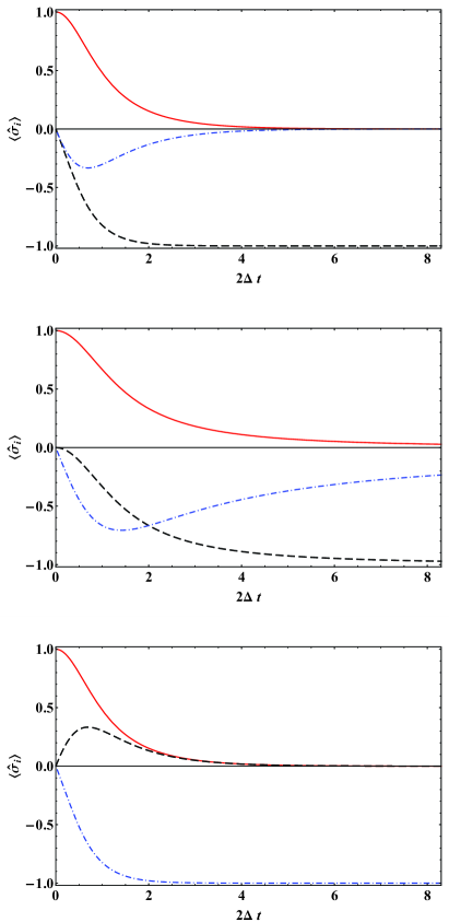
Figure 1: (Color online) Profiles of $\left\langle\hat{\sigma}_{x}\right\rangle$ (solid line), $\left\langle\hat{\sigma}_{y}\right\rangle$ (dashed line) and $\left\langle\hat{\sigma}_{z}\right\rangle$ (dot-dashed line) for the “on-shell” value $\nu=0$ and, from top to bottom, $a_{2}=1,0,-1$. The curves for ${\cal C}_{\sigma_{x}\sigma_{x}}$ and ${\cal C}_{\sigma_{x}\sigma_{x}}^{(L)}$ coincide with $\left\langle\hat{\sigma}_{x}\right\rangle$.

Finally, it should be mentioned that notwithstanding the mathematical equivalence of the evolution equations, which underlie the definitions of the correlation functions, these definitions themselves represent different physical points of view. The definition given in Eq. (15) (whose special cases are found in Eqs. (10) and (12)), implies that the actual time evolution is driven by the normalized density operator $\hat{\rho}$ whereas the non-normalized density $\hat{\Omega}$ is an auxiliary quantity. The definition given in Eq. (16) (whose special cases are found in Eqs. (11) and (13)), is based on the alternative point of view: it is the non-normalized density operator that actually drives the time evolution.

IV Correlations in two-level systems

In this section we consider as a specific example a number of non-Hermitian TLS models, which were already studied in Ref. sz13 . For these models the Hermitian part is common and is described by the Hamiltonian

$$\hat{H}_{+}=-\hbar\Delta\hat{\sigma}_{x},$$ (17)

$\Delta$ being a positive-valued constant parameter, whereas the anti-Hermitian part (the so-called decay rate operator) $\hat{\Gamma}$ varies. The models of such a kind are quite general: they are often used in order to effectively describe the dissipative and measurement-related phenomena in open quantum-optical and spin systems, such as the direct photodetection of a driven TLS interacting with the electromagnetic field bpbook .

Here we are going to compute the correlation functions using the definitions in Eqs. (10) and (11). In particular, we are going to explicitly consider the case of the autocorrelation functions, defined in Eqs. (12) and (13). Some other two-time correlation functions are presented in the Appendix.

With the goal of obtaining exact analytical results, and considering the comment after Eq. (10), we restrict our study only to those initial density matrices satisfying

$${\rm tr}\left(\hat{\sigma}_{k}\hat{\rho}(0)\right)={\rm tr}\left(\hat{\sigma}_{k}\hat{\Omega}(0)\right)/{\rm tr}\hat{\Omega}(0)=1,$$ (18)

where $k=x,z$, so that $\hat{\sigma}_{k}$ will denote a Pauli matrix operator in the Schrödinger picture. The initial conditions for the density matrix, which are labelled by the index $k$, do not need to be satisfied simultaneously. In general, such conditions restrict the physical situations that one can describe. However, we are not aiming at providing a general solution of the dynamics but we want to illustrate the formalism of the correlation function, introduced in Sec. III.2, by providing several specific examples. Hence, for what follows, it is useful to define the following density matrices that satisfy (18) for $k=x,z$, respectively:

$$\hat{\rho}_{x} = \frac{1}{2}\left(I+\sigma_{x}-\nu\sigma_{y}\right)$$ (21)

$$= \frac{1}{2}\sum_{j,m=g,e}|j\rangle\langle m|+\frac{i}{2}\nu\left(\begin{array}[]{cc}0&~{}~{}1\\ -1&~{}~{}0\end{array}\right),$$

$$\hat{\rho}_{z} = \frac{1}{2}\left(I+\sigma_{z}-\nu\sigma_{y}\right)$$ (24)

$$= |e\rangle\langle e|+\frac{i}{2}\nu\left(\begin{array}[]{cc}0&~{}~{}1\\ -1&~{}~{}0\end{array}\right),$$

where $\nu$ is some real-valued constant parameter, and we use the standard qubit notations

$$|e\rangle\langle e|=\left(\begin{array}[]{cc}1&~{}~{}0\\ 0&~{}~{}0\end{array}\right),\ \ \sum_{j,m=g,e}|j\rangle\langle m|=\left(\begin{array}[]{cc}1&~{}~{}1\\ 1&~{}~{}1\end{array}\right).$$

In order to describe physical situations, the initial conditions (21) and (24) must be supplemented with the condition of positive semi-definiteness of the density matrix $\hat{\rho}(0)$. In this case, such a condition is equivalent to

$$\nu=0.$$ (25)

The condition in Eq. (25), relating the value of the parameter $\nu$ to the positive semi-definiteness of the density matrix at the initial time, can be deduced by inspecting the eigenvalues of the density matrices in Eqs. (21) and (24):

$$\lambda_{\pm}[\hat{\rho}_{x}]=\lambda_{\pm}[\hat{\rho}_{z}]=\frac{1}{2}\left(1\pm\sqrt{1+\nu^{2}}\right).$$ (26)

In what follows we will call Eq. (25) the “on-shell” condition: it makes sure that the probabilistic interpretation of the density operator is preserved. Hence, the parameter $\nu$ can be regarded as a measure of the deviation of the solutions from those that are physically permitted. However, as it will be explained in detail later, it is convenient to first obtain the solutions “off-shell” (i.e., at $\nu\not=0$).

IV.1 Evolution with conserved average energy (exponential decay)

Let us consider the model specified by the sum of the Hermitian Hamiltonian in Eq. (17) and the anti-Hermitian part given by

$$\hat{\Gamma}^{\text{(ed)}}=\hbar\Delta\left(a_{2}\hat{\sigma}_{y}+\hat{\sigma}_{z}+\gamma\hat{I}\right),$$ (27)

where $a_{2}$ and $\gamma$ are two constant parameters. This model was considered in section 4.1 of sz13 .

As discussed previously, in order to compute analytically the autocorrelation functions ${\cal C}_{\sigma_{x}\sigma_{x}}$ and ${\cal C}_{\sigma_{x}\sigma_{x}}^{(L)}$, defined as in (12) and (13), we must impose the initial conditions in Eq. (21) on the density operator. As a result, the analytical expressions of the averages of the spin operators have the following form:

$$\langle\hat{\sigma}_{x}\rangle=\frac{a_{2}^{2}}{S^{(\text{ed})}_{\nu}(t)},$$ (28)

$$\langle\hat{\sigma}_{y}\rangle=\frac{1}{S^{(\text{ed})}_{\nu}(t)}\biggl{[}(\nu(1-a_{2}^{2})-1)\cosh{(\alpha t)}$$

$$\qquad\qquad-a_{2}^{2}\sinh{(\alpha t)}+1-\nu\biggr{]},$$ (29)

$$\langle\hat{\sigma}_{z}\rangle=\frac{a_{2}(1-\nu)}{S^{(\text{ed})}_{\nu}(t)}\left(e^{-\alpha t}-1\right),$$ (30)

where $\alpha=2a_{2}\Delta$, and we introduced the function $S^{(\text{ed})}_{b}(t)=(a_{2}^{2}-b+1)\cosh{(\alpha t)}+a_{2}^{2}b\sinh{(\alpha t)}+b-1,$ with $b$ being an index.

It is worth noting that the observable values do not depend on the parameter $\gamma$. This arises from the independence of Eq. (5) on the absolute value of the energy, as it was already discussed in sz13 ; sz14 . Another thing to note is that the value $\langle\hat{\sigma}_{x}\rangle\propto\left\langle H_{+}\right\rangle$, though vanishing at long times (as shown below), is not identically zero, since the initial condition (21) was used. Such a condition is different from the one used in sz13 . The form of the autocorrelation functions is:

$${\cal C}_{\sigma_{x}\sigma_{x}}(t)=a_{2}^{2}\biggl{[}\left(a_{2}^{2}+i\nu a_{2}+1\right)\cosh{(\alpha t)}$$

$$\qquad\qquad\quad+i\nu a_{2}\sinh{(\alpha t)}-i\nu a_{2}-1\biggr{]}^{-1},$$ (31)

$${\cal C}_{\sigma_{x}\sigma_{x}}^{(L)}(t)=\frac{a_{2}^{2}}{S^{(\text{ed})}_{\nu}(t)}=\langle\hat{\sigma}_{x}\rangle.$$ (32)

The long-time asymptotic values of Eqs. (28) - (32) are:

$$\lim\limits_{t\to+\infty}\langle\hat{\sigma}_{x}\rangle=0,$$ (33)

$$\lim\limits_{t\to+\infty}\langle\hat{\sigma}_{y}\rangle=-\left(\frac{1-a_{2}^{2}}{1+a_{2}^{2}}\right)^{\theta(-\alpha)},$$ (34)

$$\lim\limits_{t\to+\infty}\langle\hat{\sigma}_{z}\rangle=\frac{2\theta(-\alpha)a_{2}}{1+a_{2}^{2}},$$ (35)

$$\lim\limits_{t\to+\infty}{\cal C}_{\sigma_{x}\sigma_{x}}(t)=\lim\limits_{t\to+\infty}{\cal C}_{\sigma_{x}\sigma_{x}}^{(L)}(t)=0,$$ (36)

where $\theta(x)$ is the Heaviside step function. The comparative plots of different observables for some values of the parameters are shown in Fig. 1.

In order to compute analytically the autocorrelation functions ${\cal C}_{\sigma_{z}\sigma_{z}}$ and ${\cal C}_{\sigma_{z}\sigma_{z}}^{(L)}$, the initial condition in Eq. (24) is imposed. As a result, the analytical expressions of the averages of the spin operators have the form:

$$\langle\hat{\sigma}_{x}\rangle=0,$$ (37)

$$\langle\hat{\sigma}_{y}\rangle=\frac{a_{2}-1}{T^{(\text{ed})}_{\nu}(t)}\biggl{[}(1-\nu(a_{2}+1))\cosh{(\alpha t)}$$

$$\qquad\quad-a_{2}\sinh{(\alpha t)}-\frac{\nu}{a_{2}-1}-1\biggr{]},$$ (38)

$$\langle\hat{\sigma}_{z}\rangle=\frac{a_{2}(1-\nu)}{T^{(\text{ed})}_{\nu}(t)}\left(e^{-\alpha t}+\frac{a_{2}}{1-\nu}-1\right),$$ (39)

where we introduced the function $T^{(\text{ed})}_{b}(t)=(a_{2}^{2}-a_{2}-b+1)\cosh{(\alpha t)}-a_{2}(1-a_{2}b)\sinh{(\alpha t)}+a_{2}+b-1.$ The form of the corresponding autocorrelation functions is:

$${\cal C}_{\sigma_{z}\sigma_{z}}(t)=\frac{a_{2}}{T^{(\text{ed})}_{0}(t)}\left(e^{-\alpha t}+a_{2}-1\right),$$ (40)

$${\cal C}_{\sigma_{z}\sigma_{z}}^{(L)}(t)=\frac{a_{2}}{T^{(\text{ed})}_{\nu}(t)}\left(e^{-\alpha t}+a_{2}-1\right).$$ (41)

The long-times asymptotic values of Eqs. (37) - (41) are:

$$\lim\limits_{t\to+\infty}\langle\hat{\sigma}_{x}\rangle=0,$$ (42)

$$\lim\limits_{t\to+\infty}\langle\hat{\sigma}_{y}\rangle=-\left(\frac{1-a_{2}^{2}}{1+a_{2}^{2}}\right)^{\theta(-\alpha)},$$ (43)

$$\lim\limits_{t\to+\infty}\langle\hat{\sigma}_{z}\rangle=\frac{2\theta(-\alpha)a_{2}}{1+a_{2}^{2}},$$ (44)

$$\lim\limits_{t\to+\infty}{\cal C}_{\sigma_{z}\sigma_{z}}(t)=\frac{2\theta(-\alpha)a_{2}}{1+a_{2}^{2}},$$ (45)

$$\lim\limits_{t\to+\infty}{\cal C}_{\sigma_{z}\sigma_{z}}^{(L)}(t)=\frac{2\theta(-\alpha)a_{2}}{1+a_{2}^{2}}\frac{1}{1-\nu}.$$ (46)

In this set of solutions, it is clear that the autocorrelation function ${\cal C}_{\sigma_{z}\sigma_{z}}^{(L)}(t)$ depends on the initial conditions. It is also worth noticing that the ratio

$$\frac{\lim\limits_{t\to+\infty}{\cal C}_{\sigma_{z}\sigma_{z}}(t)}{\lim\limits_{t\to+\infty}{\cal C}_{\sigma_{z}\sigma_{z}}^{(L)}(t)}=1-\nu$$

does not depend on the parameters of the Hamiltonian but it depends on the parameter $\nu$ whose nature was discussed after Eq. (26).

The comparative plots of different observables for some values of parameters are shown in Fig. 2. It is easy to see that the difference between the two functions ${\cal C}_{\sigma_{k}\sigma_{k}}(t)$, and ${\cal C}^{(L)}_{\sigma_{k}\sigma_{k}}(t)$, for each case $k=x,z$, disappears when $\nu\to 0$. The implications of this feature are discussed in Sec. V.

IV.2 Evolution with conserved average energy (polynomial decay)

Here, we consider the model specified by the sum of the Hermitian Hamiltonian Eq. (17) and the anti-Hermitian part given by

$$\hat{\Gamma}^{\text{(pd)}}=\hbar\Delta\left(\hat{\sigma}_{z}+\gamma\hat{I}\right),$$ (47)

where the parameter $\gamma$ is specified as in Sec. IV.1. This model was considered in section 4.2 of sz13 .

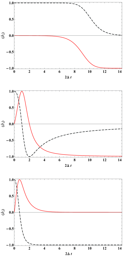
Figure 2: (Color online) Profiles of $\left\langle\hat{\sigma}_{y}\right\rangle$ (solid line) and $\left\langle\hat{\sigma}_{z}\right\rangle$ (dashed line) for the “on-shell” value $\nu=0$ and, from top to bottom, $a_{2}=1.0001,0,-1$. The value $\left\langle\hat{\sigma}_{x}\right\rangle$ is identically zero, and the curves for ${\cal C}_{\sigma_{x}\sigma_{x}}$ and ${\cal C}_{\sigma_{x}\sigma_{x}}^{(L)}$ coincide with $\left\langle\hat{\sigma}_{z}\right\rangle$.

As discussed previously, in order to compute analytically the autocorrelation functions ${\cal C}_{\sigma_{x}\sigma_{x}}$ and ${\cal C}_{\sigma_{x}\sigma_{x}}^{(L)}$, we use the initial condition specified by Eq. (21) on the density operator. Consequently, the analytical expressions of the averages of the spin operators have the form

$$\langle\hat{\sigma}_{x}\rangle=0,$$ (48)

$$\langle\hat{\sigma}_{y}\rangle=\frac{1-\nu}{S^{(\text{pd})}_{\nu}(t)}-1,$$ (49)

$$\langle\hat{\sigma}_{z}\rangle=\frac{2\Delta(\nu-1)t}{S^{(\text{pd})}_{\nu}(t)},$$ (50)

where we introduced the function $S^{(\text{pd})}_{b}(t)=2\Delta^{2}(1-b)t^{2}+1$. The form of the autocorrelation functions is:

$${\cal C}_{\sigma_{x}\sigma_{x}}(t)=\left[S^{(\text{pd})}_{0}(t)+2i\nu\Delta\,t\right]^{-1},$$ (51)

$${\cal C}_{\sigma_{x}\sigma_{x}}^{(L)}(t)=1/S^{(\text{pd})}_{\nu}(t).$$ (52)

The long-times asymptotic values of Eqs. (48) - (52) are:

$$\lim\limits_{t\to+\infty}\langle\hat{\sigma}_{x}\rangle=\lim\limits_{t\to+\infty}\langle\hat{\sigma}_{z}\rangle=0,$$ (53)

$$\lim\limits_{t\to+\infty}\langle\hat{\sigma}_{y}\rangle=-1,$$ (54)

$$\lim\limits_{t\to+\infty}{\cal C}_{\sigma_{x}\sigma_{x}}(t)=\lim\limits_{t\to+\infty}{\cal C}_{\sigma_{x}\sigma_{x}}^{(L)}(t)=0.$$ (55)

The graphs of different observables, corresponding to some values of the parameters, can be found in the middle plot of Fig. 1.

In order to compute analytically the autocorrelation functions ${\cal C}_{\sigma_{z}\sigma_{z}}$ and ${\cal C}_{\sigma_{z}\sigma_{z}}^{(L)}$, we impose the initial condition given by Eq. (24) on the density operator. It follows that the analytical expressions of the averages of the spin operators are:

$$\langle\hat{\sigma}_{x}\rangle=0,$$ (56)

$$\langle\hat{\sigma}_{y}\rangle=\frac{1-\nu}{T^{(\text{pd})}_{\nu}(t)}-1,$$ (57)

$$\langle\hat{\sigma}_{z}\rangle=\frac{1-2\Delta(1-\nu)t}{T^{(\text{pd})}_{\nu}(t)},$$ (58)

where $T^{(\text{pd})}_{b}(t)=2\Delta\left[\Delta(1-b)t-1\right]t+1$. The autocorrelation functions have the form

$${\cal C}_{\sigma_{z}\sigma_{z}}(t)=\frac{1-2\Delta\,t}{T^{(\text{pd})}_{0}(t)},$$ (59)

$${\cal C}_{\sigma_{z}\sigma_{z}}^{(L)}(t)=\frac{1-2\Delta\,t}{T^{(\text{pd})}_{\nu}(t)}.$$ (60)

The long-times asymptotic values of Eqs. (56) - (60) are:

$$\lim\limits_{t\to+\infty}\langle\hat{\sigma}_{x}\rangle=\lim\limits_{t\to+\infty}\langle\hat{\sigma}_{z}\rangle=0,$$ (61)

$$\lim\limits_{t\to+\infty}\langle\hat{\sigma}_{y}\rangle=-1,$$ (62)

$$\lim\limits_{t\to+\infty}{\cal C}_{\sigma_{z}\sigma_{z}}(t)=0,$$ (63)

$$\lim\limits_{t\to+\infty}{\cal C}_{\sigma_{z}\sigma_{z}}^{(L)}(t)=\delta_{1\nu},$$ (64)

where $\delta_{ab}$ is the Kronecker symbol.

The graphs of different observables, corresponding to some values of the parameters, can be found in the middle plot in Fig. 2. As before, the difference between the two functions ${\cal C}_{\sigma_{k}\sigma_{k}}(t)$ and ${\cal C}^{(L)}_{\sigma_{k}\sigma_{k}}(t)$ for each case $k=x,z$ disappears when $\nu\to 0$. The implications of this feature are discussed in Sec. V.

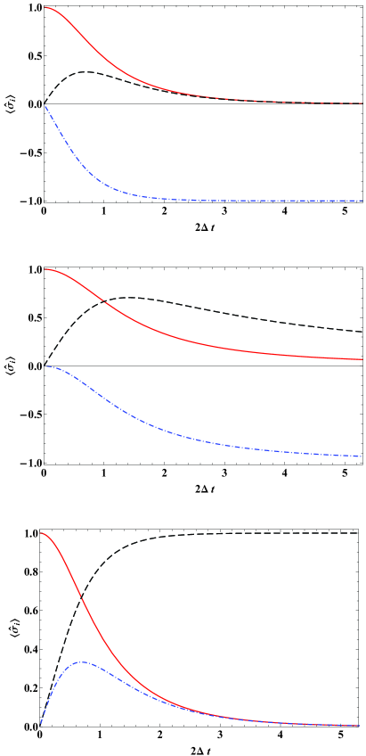
Figure 3: (Color online) Profiles of $\left\langle\hat{\sigma}_{x}\right\rangle$ (solid line), $\left\langle\hat{\sigma}_{y}\right\rangle$ (dashed line) and $\left\langle\hat{\sigma}_{z}\right\rangle$ (dot-dashed line) for the “on-shell” value $\nu=0$ and, from top to bottom, $\gamma=1,0,-1$. The curves for ${\cal C}_{\sigma_{x}\sigma_{x}}$ and ${\cal C}_{\sigma_{x}\sigma_{x}}^{(L)}$ coincide with $\left\langle\hat{\sigma}_{x}\right\rangle$.

IV.3 Evolution with asymptotic dephasing

Let us consider the model specified by the sum of the Hermitian Hamiltonian in Eq. (17) and the anti-Hermitian part given by

$$\hat{\Gamma}^{(\text{dph})}=-\hbar\Delta\left[\hat{\sigma}_{y}-\gamma\left(\hat{\sigma}_{z}+\hat{I}\right)\right],$$ (65)

where $\gamma$ is a constant parameter. This model was proposed in section 6 of sz13 . Since in Eq. (65) the parameter $\gamma$ does not appear only in the $\hat{I}$ term, it is going to appear in all of the expressions for the observables.

As discussed previously, in order to compute analytically the autocorrelation functions ${\cal C}_{\sigma_{x}\sigma_{x}}$ and ${\cal C}_{\sigma_{x}\sigma_{x}}^{(L)}$, we use the initial condition specified by Eq. (21) on the density operator. Consequently, solving the evolution equation yields the following components of the (non-normalized) density matrix:

$$(\hat{\Omega})_{11}=\frac{1}{2}e^{-2\Gamma t}\;,$$ (66)

$$(\hat{\Omega})_{12}=(\hat{\Omega})_{21}^{*}=\frac{e^{-2\Gamma t}}{2\gamma}\left[(\gamma+i(\nu\gamma-1))e^{\Gamma t}+i\right]\!,~{}~{}~{}$$ (67)

$$(\hat{\Omega})_{22}=\frac{\left(e^{-\Gamma t}-1\right)^{2}+2\nu\gamma\left(e^{-\Gamma t}-1\right)+\gamma^{2}}{2\gamma^{2}},$$ (68)

where $\Gamma=2\gamma\Delta$. It is worth recalling that for the model given by Eqs. (17) and (65), the off-diagonal components of the density matrix vanish at long times. Furthermore, the analytical expressions of the averages of the spin operators have the form:

$$\langle\hat{\sigma}_{x}\rangle=\frac{\gamma^{2}}{S^{(\text{dph})}_{\nu}(t)},$$ (69)

$$\langle\hat{\sigma}_{y}\rangle=\frac{\gamma}{S^{(\text{dph})}_{\nu}(t)}\left(1-\nu\gamma-e^{-\Gamma t}\right),$$ (70)

$$\langle\hat{\sigma}_{z}\rangle=\frac{\gamma^{2}e^{-\Gamma t}}{S^{(\text{dph})}_{\nu}(t)}-1,$$ (71)

where $\tilde{\gamma}^{2}=\gamma^{2}+1$ and we have introduced the function $S^{(\text{dph})}_{b}(t)=(\tilde{\gamma}^{2}-b\gamma)\cosh{(\Gamma t)}-b\gamma\sinh{(\Gamma t)}+b\gamma-1.$ The autocorrelation functions have the form:

$${\cal C}_{\sigma_{x}\sigma_{x}}(t)=\frac{\gamma^{2}}{S^{(\text{dph})}_{0}(t)+i\nu\left[\gamma^{2}\sinh{(\Gamma t)}-\cosh{(\Gamma t)}+1\right]},$$ (72)

$${\cal C}_{\sigma_{x}\sigma_{x}}^{(L)}(t)=\frac{\gamma^{2}}{S^{(\text{dph})}_{\nu}(t)}.$$ (73)

The long-time asymptotic values of Eqs. (69-73) are:

$$\lim\limits_{t\to+\infty}\langle\hat{\sigma}_{x}\rangle=0,$$ (74)

$$\lim\limits_{t\to+\infty}\langle\hat{\sigma}_{y}\rangle=-\frac{2\gamma\theta(-\Gamma)}{\tilde{\gamma}^{2}},$$ (75)

$$\lim\limits_{t\to+\infty}\langle\hat{\sigma}_{z}\rangle=-\left(\frac{1-\gamma^{2}}{\tilde{\gamma}^{2}}\right)^{\theta(-\Gamma)}\!,~{}~{}~{}$$ (76)

$$\lim\limits_{t\to+\infty}{\cal C}_{\sigma_{x}\sigma_{x}}(t)=\lim\limits_{t\to+\infty}{\cal C}_{\sigma_{x}\sigma_{x}}^{(L)}(t)=0,$$ (77)

where the function $\theta(x)$ has been defined in Sec. IV.1. The comparative plots of different observables for some values of parameters are shown in Fig. 3.

In order to compute analytically the autocorrelation functions ${\cal C}_{\sigma_{z}\sigma_{z}}$ and ${\cal C}_{\sigma_{z}\sigma_{z}}^{(L)}$, the initial condition in Eq. (24) is imposed. As a result, the analytical expressions of the averages of the spin operators have the form:

$$\langle\hat{\sigma}_{x}\rangle=0,$$ (78)

$$\langle\hat{\sigma}_{y}\rangle=\frac{\gamma}{T^{(\text{dph})}_{\nu}(t)}\left(2-\nu\gamma-2e^{-\Gamma t}\right),$$ (79)

$$\langle\hat{\sigma}_{z}\rangle=\frac{2\gamma^{2}e^{-\Gamma t}}{T^{(\text{dph})}_{\nu}(t)}-1,$$ (80)

where we have introduced the function $T^{(\text{dph})}_{b}(t)=(\tilde{\gamma}^{2}-b\gamma+1)\cosh{(\Gamma t)}-\gamma(\gamma+b)\sinh{(\Gamma t)}+b\gamma-2.$ The autocorrelation functions have the form:

$${\cal C}_{\sigma_{z}\sigma_{z}}(t)=\frac{4(1-\cosh{(\Gamma t)})}{T^{(\text{dph})}_{0}(t)}+1,$$ (81)

$${\cal C}_{\sigma_{z}\sigma_{z}}^{(L)}(t)=\frac{T^{(\text{dph})}_{0}+4(1-\cosh{(\Gamma t)})}{T^{(\text{dph})}_{\nu}(t)}.$$ (82)

The long-time asymptotic values of Eqs. (78-82) are:

$$\lim\limits_{t\to+\infty}\langle\hat{\sigma}_{x}\rangle=0,$$ (83)

$$\lim\limits_{t\to+\infty}\langle\hat{\sigma}_{y}\rangle=-\frac{2\gamma\theta(-\Gamma)}{\tilde{\gamma}^{2}},$$ (84)

$$\lim\limits_{t\to+\infty}\langle\hat{\sigma}_{z}\rangle=\lim\limits_{t\to+\infty}{\cal C}_{\sigma_{z}\sigma_{z}}(t)=-\left(\frac{1-\gamma^{2}}{\tilde{\gamma}^{2}}\right)^{\theta(-\Gamma)}\!,~{}~{}~{}~{}~{}$$ (85)

$$\lim\limits_{t\to+\infty}{\cal C}_{\sigma_{z}\sigma_{z}}^{(L)}(t)=\begin{cases}(\nu\gamma-1)^{-1}&\text{if }\Gamma>0,\\ \left(1-\gamma^{2}\right)/\tilde{\gamma}^{2}&\text{if }\Gamma<0,\end{cases}$$ (86)

where $\theta(x)$ has been defined in Sec. IV.1.

The comparative plots of different observables for some values of parameters are shown in Fig. 4. As in the previous sections, the difference between the two functions ${\cal C}_{\sigma_{k}\sigma_{k}}(t)$ and ${\cal C}^{(L)}_{\sigma_{k}\sigma_{k}}(t)$ for each case $k=x,z$ disappears when $\nu\to 0$. The possible implications of this feature shall be discussed in the next section.

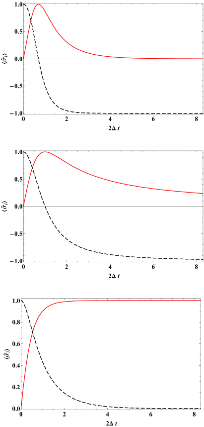
Figure 4: (Color online) Profiles of $\left\langle\hat{\sigma}_{y}\right\rangle$ (solid line) and $\left\langle\hat{\sigma}_{z}\right\rangle$ (dashed line) for the “on-shell” value $\nu=0$ and, from top to bottom, $\gamma=1,0,-1$. The value $\left\langle\hat{\sigma}_{x}\right\rangle$ is identically zero, and the curves for ${\cal C}_{\sigma_{x}\sigma_{x}}$ and ${\cal C}_{\sigma_{x}\sigma_{x}}^{(L)}$ coincide with $\left\langle\hat{\sigma}_{z}\right\rangle$.

V Discussion and Conclusion

Having as a final goal the proper foundation of the statistical mechanics of systems with non-Hermitian Hamiltonians (which is a research endeavor that we started in Ref. sz13 ), in this paper we have introduced a formalism for multi-time correlation functions. The approach is general: it depends neither on the number of degrees of freedom in the system nor on the dimensionality of the Hilbert space itself; it is also valid if the degrees of freedom are continuous. We have found that such a formalism can lead to two different definitions of the time correlation function. Notwithstanding the equivalence of the evolution equations underlying these definitions, the different time correlation functions represent distinct physical points of view. The first definition is presented in Eq. (15) and its special cases are given by Eqs. (10) and (12). Such a definition presumes that the actual dynamics is defined in terms of the normalized density operator. The second definition is presented in Eq. (16) and its special cases are given by Eqs. (11) and (13). Alternatively, this second definition assumes that the dynamics is defined in terms of the non-normalized density operator.

In the case of one-point time correlation functions (which provide basically statistical averages), both definitions lead to the same results. However, in general (i.e., for multiple-time correlation functions), the two definitions do not coincide, as it has been illustrated by explicitly studying various two-level models.

As we have already remarked at the end of Secs. IV.1-IV.3, the relative difference between the two definitions of autocorrelation functions, $\Delta{\cal C}_{i}=1-{\cal C}_{\sigma_{i}\sigma_{i}}/{\cal C}_{\sigma_{i}\sigma_{i}}^{(L)}$ ($i=x,y,z$), tends to zero when $\nu$ approaches the “on-shell” value (25), at any time $t$. As it is known, the probabilistic interpretation of a density operator requires the matrices (21) and (24) to be positive semi-definite. The parameter $\nu$ indicates the deviation from such a property, as it has been discussed after Eq. (26). Therefore, one can naturally propose the conjecture that functions such as $\Delta{\cal C}_{i}$ are useful in order to assess the positive semi-definiteness of the density operator without actually computing its eigenvalues. In particular, such a conjecture could be especially useful when the number of density matrix’s eigenvalues is rather large (e.g., when the Hilbert space is infinite). In this paper, we have verified by studying various two-level models that, indeed, the positive semi-definiteness of the density matrix holds whenever the functions $\Delta{\cal C}_{i}$ vanish. The further investigation of this problem is an interesting direction of future work.

Appendix A Other correlation functions for TLS

Apart from the autocorrelation functions computed in Sec. IV, one can of course compute other types of correlation functions, for each of the two-level systems we have considered above. For instance, below we present the two-time correlations ${\cal C}_{\sigma_{z}\sigma_{x}}$, ${\cal C}_{\sigma_{z}\sigma_{x}}^{(L)}$, ${\cal C}_{\sigma_{z}\sigma_{y}}$ and ${\cal C}_{\sigma_{z}\sigma_{y}}^{(L)}$, where we assume the notation:

$${\cal C}_{\xi\chi}(t)={\rm tr}\left\{\hat{\chi}{\cal K}(t,0)\hat{\xi}\hat{\rho}(0)\right\},$$ (87)

$${\cal C}^{(L)}_{\xi\chi}(t)=\frac{{\rm tr}\left\{\hat{\chi}{\cal K}_{L}(t,0)\hat{\xi}\hat{\Omega}(0)\right\}}{{\rm tr}\,\hat{\Omega}(t)},$$ (88)

and set the initial time to zero, which is equivalent to all times being counted from the moment $t=t_{0}=t_{1}$.

Further, as long as the operator, which is first from the right in the definitions of functions ${\cal C}_{\sigma_{z}\sigma_{x}}$, ${\cal C}_{\sigma_{z}\sigma_{x}}^{(L)}$, ${\cal C}_{\sigma_{z}\sigma_{y}}$ and ${\cal C}_{\sigma_{z}\sigma_{y}}^{(L)}$, is $\hat{\sigma}_{z}$, below we are going to use $\hat{\rho}_{z}$, as defined in Eq. (24), as the initial value for the density operator, for the reasons specified above.

A.1 Evolution with conserved average energy (exponential decay)

For the model from Sec. IV.1 we obtain

$${\cal C}_{\sigma_{z}\sigma_{x}}(t)=\frac{ia_{2}^{2}\nu}{T^{(\text{ed})}_{0}(t)},$$ (89)

$${\cal C}_{\sigma_{z}\sigma_{x}}^{(L)}(t)=\frac{ia_{2}^{2}\nu}{T^{(\text{ed})}_{\nu}(t)},$$ (90)

and

$${\cal C}_{\sigma_{z}\sigma_{y}}(t)=\frac{a_{2}-1}{T^{(\text{ed})}_{0}(t)}\left[\cosh{(\alpha t)}-a_{2}\sinh{(\alpha t)}-1\right]\!,~{}~{}~{}~{}~{}~{}$$ (91)

$${\cal C}_{\sigma_{z}\sigma_{y}}^{(L)}(t)=\frac{a_{2}-1}{T^{(\text{ed})}_{\nu}(t)}\left[\cosh{(\alpha t)}-a_{2}\sinh{(\alpha t)}-1\right]\!,$$ (92)

where we have used the notation from Sec. IV.1.

A.2 Evolution with conserved average energy (polynomial decay)

For the model from Sec. IV.2 we obtain

$${\cal C}_{\sigma_{z}\sigma_{x}}(t)=\frac{i\nu}{T^{(\text{pd})}_{0}(t)},$$ (93)

$${\cal C}_{\sigma_{z}\sigma_{x}}^{(L)}(t)=\frac{i\nu}{T^{(\text{pd})}_{\nu}(t)},$$ (94)

and

$${\cal C}_{\sigma_{z}\sigma_{y}}(t)=\frac{2\Delta(1-\Delta\,t)t}{T^{(\text{pd})}_{0}(t)},$$ (95)

$${\cal C}_{\sigma_{z}\sigma_{y}}^{(L)}(t)=\frac{2\Delta(1-\Delta\,t)t}{T^{(\text{pd})}_{\nu}(t)},$$ (96)

where the notation of Sec. IV.2 is implied.

A.3 Evolution with asymptotic dephasing

For the model from Sec. IV.3 we obtain

$${\cal C}_{\sigma_{z}\sigma_{x}}(t)=\frac{i\gamma^{2}\nu}{T^{(\text{dph})}_{0}(t)},$$ (97)

$${\cal C}_{\sigma_{z}\sigma_{x}}^{(L)}(t)=\frac{i\gamma^{2}\nu}{T^{(\text{dph})}_{\nu}(t)},$$ (98)

and

$${\cal C}_{\sigma_{z}\sigma_{y}}(t)=\frac{2\gamma(1-e^{-\Gamma t})}{T^{(\text{dph})}_{0}(t)},$$ (99)

$${\cal C}_{\sigma_{z}\sigma_{y}}^{(L)}(t)=\frac{2\gamma(1-e^{-\Gamma t})}{T^{(\text{dph})}_{\nu}(t)},$$ (100)

where the notation of Sec. IV.3 is implied.

References

- (1) H. Suura, Prog. Theor. Phys. 12 49-71 (1954).
- (2) F. Coester and H. Kümmel, Nucl. Phys. 9 225-236 (1958).
- (3) A. J. Layzer, Phys. Rev. 129 908-925 (1963).
- (4) C. M. Bender, Rep. Prog. Phys. 70 947 (2007).
- (5) B. D. Wibking and K. Varga, Phys. Lett. A 376 365 (2012).
- (6) K.-F. Berggreen, I. I. Yakimenko, and J. Hakanen, New. J. Phys. 12 073005 (2010).
- (7) M. Znojil, Phys. Rev. D 80 045009 (2009).
- (8) K. Varga and S. T. Pantelides, Phys. Rev. Lett. 98 076804 (2007).
- (9) J.G. Muga, J.P. Palao, B. Navarro, and I.L. Egusquiza, Phys. Rep. 395 357 (2004).
- (10) A. Thilagam, J. Chem. Phys. 136 065104 (2011).
- (11) N. Moiseyev, Phys. Rep. 302 211 (1998).
- (12) W. John, B. Milek, H. Schanz, and P. Seba, Phys. Rev. Lett. 67 1949 (1991).
- (13) C. A. Nicolaides and S. I. Themelis Phys. Rev. A 45 349 (1992).
- (14) H. Feshbach, Ann. Phys. (N.Y.) 5 357 (1958); 19 287 (1962).
- (15) E. C. G. Sudarshan, C. B. Chiu, and V. Gorini, Phys. Rev. D 18 2914 (1978).
- (16) S. Selstø, T. Birkeland, S. Kvaal, R. Nepstad, and M. Førre, J. Phys. B: At. Mol. Opt. Phys. 44 215003 (2011).
- (17) H. C. Baker, Phys. Rev. Lett. 50 1579-1582 (1983).
- (18) H. C. Baker, Phys. Rev. A 30 773 (1984).
- (19) S.-I. Chu and W. P. Reinhardt, Phys. Rev. Lett. 39 1195 (1977).
- (20) C. E. Rüter, K. G. Makris, R. El-Ganainy, D. N. Christodoulides, M. Segev, and D. Kip, Nat. Phys. 6 192 (2010).
- (21) A. Guo, G. J. Salamo, D. Duchesne, R. Morandotti, M. Volatier-Ravat, V. Aimez, G. A. Siviloglou, and D. N. Christodoulides, Phys. Rev. Lett. 103 093902 (2009).
- (22) J. Korringa, Phys. Rev. 133 1228 (1964).
- (23) J. Wong, J. Math. Phys. 8 2039 (1967).
- (24) G. C. Hegerfeldt, Phys. Rev. A 47 449 (1993).
- (25) S. Baskoutas, A. Jannussis, R. Mignani, and V. Papatheou, J. Phys. A: Math. Gen. 26 L819 (1993).
- (26) P. Angelopoulou, S. Baskoutas, A. Jannussis, R. Mignani, and V. Papatheou, Int. J. Mod. Phys. B 9 2083 (1995).
- (27) I. Rotter, arXiv:0711.2926.
- (28) I. Rotter, J. Phys. A 42 153001 (2009).
- (29) H. B. Geyer, F. G. Scholtz and K. G. Zloshchastiev, Proceedings of 12th International Conference on Mathematical Methods in Electromagnetic Theory (IEEE, Piscataway, 2008), pp. 250–252.
- (30) R. Lo Franco, B. Bellomo, S. Maniscalco, and G. Compagno, Int. J. Mod. Phys. B 27 1345053 (2013).
- (31) S. Banerjee and R. Srikanth, Mod. Phys. Lett. B 24 2485 (2010).
- (32) F. Reiter and A. S. Sørensen, Phys. Rev. A 85 032111 (2012).
- (33) A. Sergi and K. G. Zloshchastiev, Int. J. Mod. Phys. B 27 1350163 (2013) [arXiv:1207.4877].
- (34) D. C. Brody and E.-M. Graefe, Phys. Rev. Lett. 109 230405 (2012) [arXiv:1208.5297].
- (35) K. G. Zloshchastiev and A. Sergi, J. Mod. Optics 61 1298-1308 (2014) [arXiv:1405.7165].
- (36) E.-M. Graefe, M. Höning, and H. J. Korsch, J. Phys. A 43 075306 (2010).
- (37) A. Sergi, Commun. Theor. Phys. 56 96 (2011).
- (38) E.-M. Graefe and R. Schubert, Phys. Rev. A 83 060101 (2011); J. Phys. A 45 244033 (2012).
- (39) F. G. Scholtz, H. B. Geyer, and F. J. W. Hahne, Ann. Phys. (N.Y.) 213 74-101 (1992).
- (40) C. M. Bender, S. Boettcher, and P. N. Meisinger, J. Math. Phys. 40 2201 (1999).
- (41) M. Znojil, J. Nonlin. Math. Phys. 9 122-133 (2002).
- (42) A. Mostafazadeh, Int. J. Geom. Methods Mod. Phys. 7 1191 (2010).
- (43) C. W. Gardiner and P. Zoller, Quantum Noise (Springer, Berlin, 2000).
- (44) H.-P. Breuer and F. Petruccione, The Theory of Open Quantum Systems (Oxford University Press, Oxford, 2002).