Systematic approximation for QCD at non-zero density

Abstract:

We use the heavy dense formulation of QCD (HD-QCD) as the basis for an analytic expansion as systematic approximation to QCD at non-zero density, keeping the full Yang-Mills action. We analyse the structure of the baryonic density and other quantities and present data from the complex Langevin equation (CLE) and reweighting (RW) calculations for 2 flavours of Wilson fermions.

1 HD-QCD as basis for a systematic analytic approximation to QCD

The QCD grand canonical partition function for $n_{f}=1$ flavour of Wilson fermions is:

$$Z = \int DU\,\rho,\quad\rho=\rm e\,^{-S}=\rm e\,^{-S_{YM}}\det M$$ (1)

$${\rm M} = 1-2\,\kappa\sum_{i=1}^{3}\left(\Gamma_{+i}U_{x,i}T_{i}+\Gamma_{-i}U_{x,i}^{\dagger}T_{-i}\right)-2\,\kappa\gamma\left(\rm e\,^{\mu}\Gamma_{+4}U_{x,4}T_{4}+\rm e\,^{-\mu}\Gamma_{-4}U_{x,4}^{\dagger}T_{-4}\right)$$ (2)

with $\Gamma_{\pm\mu}=\frac{1}{2}(1\pm\gamma_{\mu})$, $T$: lattice translations, $\kappa$: hopping parameter, $\mu$ chemical potential, $\gamma$: anisotropy parameter. The temperature is introduced as $\ aT=\frac{\gamma}{N_{\tau}}\$ ($\gamma=1$ below).

HD-QCD [1, 2, 3] relies on the double limit

$$\kappa\rightarrow 0,\ \mu\rightarrow\infty,\ \ \zeta=2\kappa\,\rm e\,^{\mu}\,:fixed\,.$$ (3)

In the 0-th order in $\kappa$ (LO) only the Polyakov loops $P$ survive in the loop expansion for the fermionic deteminant which becomes a product of local terms

$$\det{\rm M}^{0}(\mu)=\left(1+C^{3}\right)^{2}\left(1+{C^{\prime}}^{3}\right)^{2}\prod_{\vec{x}}\left(1+a\,P_{\vec{x}}+b\,P_{\vec{x}}^{\prime}\right)^{2}\left(1+{\tilde{a}}\,P_{\vec{x}}^{\prime}+{\tilde{b}}\,P_{\vec{x}}\right)^{2}\$$ (4)

$$a=3C/(1+C^{3}),\,b=3C^{2}/(1+C^{3}),\,{\tilde{a}}=3C^{\prime}/(1+{C^{\prime}}^{3}),\,{\tilde{b}}=3{C^{\prime}}^{2}/(1+{C^{\prime}}^{3})$$ (5)

$$C=\left(2\kappa\rm e\,^{\mu}\right)^{N_{\tau}},\ \ C^{\prime}=\left(2\kappa\rm e\,^{-\mu}\right)^{N_{\tau}},\quad P=\frac{1}{3}\hbox{tr}\prod_{t}U_{t},\ \ P^{\prime}=\frac{1}{3}\hbox{tr}\prod_{t}U_{t}^{-1}$$ (6)

where we also introduced the non-dominant factors from the inverse Polyakov loops $P^{\prime}$ to preserve the $\det{\rm M}(\mu)=[\det{\rm M}(-\mu)]^{*}$ symmetry. The LO describes gluonic interactions in a background of static charges. Note that $a,b$ have maxima of $2^{2/3}$ at $\mu=\mp\frac{1}{3N_{\tau}}-\ln(2\kappa)$.

Figure 1: HD - QCD: LO and NLO.

We can go beyond the static limit (LO) with successive N^qLO to approximate full QCD using the analytic hopping expansion.

For $q=1$ the NLO can be defined in the loop expansion using decorated Polyakov loops, for explicit formulae see [4, 5]. The determinant still factorizes, but the quarks have some mobility. Higher N^qLO become increasingly cumbersome in the loop expansion, however, because of the combinatorics. The effective expansion parameter is $N_{\tau}\kappa$.

Alternatively we can expand to higher orders ”algebraically” [6], see also [7]. In the following we use two expansions, called the $\kappa$- and the $\kappa_{s}$-expansion. To define them one separates temporal and spatial hoppings in the fermionic matrix M:

$${\rm M}\ =\ 1-\kappa Q\ =\ 1-R-\kappa_{s}S,\quad R=\kappa Q_{t},\quad S=Q_{s}$$ (7)

$$\kappa{\rm-expansion}:\quad\det{\rm M}=\exp\left\{-\sum_{n}\frac{\kappa^{n}}{n}Q^{n}\right\}$$ (8)

$$\kappa_{s}{\rm-expansion}:\quad\det{\rm M}=\det{\rm M}^{0}\exp\left\{-\sum_{n}\frac{\kappa_{s}^{n}}{n}\left(\frac{S}{1-R}\right)^{n}\right\}$$ (9)

The drifts for CLE in N^qLO can be systematically derived and used for simulations with the full YM action to any desired order $q$ [6]. In the calculations one keeps $\kappa_{s}=\kappa$.

HD-QCD has been used as a model in LO and NLO to study the phase diagram and other properties with the full YM action [4, 5, 8] and in strong coupling also to higher orders [9].

2 Simulation method

2.1 Complex Langevin Simulation

The Complex Langevin Equation (CLE) has the potential to simulate lattice models with a complex action and for which usual importance sampling fails. To develop it to a reliable method is both rewarding and tough.

The LE is a stochastic process in which the updating of the variables is achieved by addition of a drift term (or ”force”) and a suitably normalized random noise. For a complex action the drift is also complex and this automatically provides an imaginary part for the field. This implies setting up the problem in the complexification of the original manifold $R^{n}\longrightarrow C^{n}$ or $SU(n)\longrightarrow SL(n,C)$. The CLE then amounts to two related, real LE with independent noise terms - here in compact form for just one variable $z=x+i\,y$ and with $K=-\partial_{z}S(z)$:

$${\delta z(t)} = K(z)\,\delta t+\sqrt{N_{R}}\,\eta_{R}+{\rm i}\,\sqrt{N_{I}}\,\eta_{I}$$

$$\langle\eta_{R}\rangle = \langle\eta_{I}\rangle=0\,,\ \langle\eta_{R}\eta_{I}\rangle=0\,,\quad\langle\eta_{R}^{2}\rangle=\langle\eta_{I}^{2}\rangle=2\,\delta t\,,\ \,\ N_{R}-N_{I}=1$$

In the simulations we shall take $N_{I}=0$. The probability distribution $P(x,y;t)$ realized in the process evolves according to a real Fokker-Planck equation:

$$\partial_{t}P(x,y,t)=L^{T}P(x,y,t)\,,\quad L=(N_{R}\partial_{x}+{\hbox{Re}}K(z))\partial_{x}+(N_{I}\partial_{x}+{\hbox{Im}}K(z))\partial_{y}$$ (10)

One can also define a complex distribution $\rho(x,t)$

$$\partial_{t}\rho(x,t)=L^{T}_{0}\rho(x,t)\,,\quad L_{0}=(\partial_{x}+K(x))\partial_{x}$$

with the asymptotic solution $\rho(x)\simeq\exp(-S(x))$ and formally prove for the observables $O(z)$

$$\quad\int{O}(x+iy)P(x,y;t)dxdy=\int{O}(x)\rho(x;t)dx.$$

As for any method the proof of convergence depends on some conditions, for CLE these include:

- rapid decay of $P(x,y,t)$ in $y$ [10] and

- holomorphy of the drift and of the observables.

There are, moreover, a number of numerical problems, such as runaways. Many of them are due to the amplification of numerical imprecisons by unstable modes in the drift dynamics. For further discussion see, e.g., [11] and the references therein.

To deal with these problems one can use the freedom in defining the process for a given action and the symmetries of the latter. For gauge theories we set up a method (”gauge cooling”) to obtain a narrow $y-$distribution. Together with using adaptive step size this also eliminates runaways and divergences triggered by numerical imprecisions. For a review see [12].

Zeroes in the original measure $\rho(z)$ lead to a meromorphic drift. The poles in the drift can cause wrong convergence of the process, as shown in nontrivial, soluble models [13]. This problem is presently under study. In the cases of physical interest the effects due to poles do not appear quantitatively relevant, however a systematic understanding is still missing.

For QCD at $\mu\neq 0$ the method has been defined in [14] and applied, e.g., in [8, 9, 15, 16].

2.2 Reweighting

For completeness we shall briefly describe the reweighting method (RW) also applied in this study. It has been used in the HD-QCD context before [5] but without the second factor in (4) (which is $\simeq 1$ at large $\mu$ but is relevant if we want to connect to the small $\mu$ region).

We split the Boltzman factor in (1) and calculate the expectation values by reweighting

$$\rho\equiv\rm e\,^{-S_{YM}}\det M=H\,w,\quad H>0,\quad\quad\langle O\rangle_{\rho}=\frac{\langle O\,w\rangle_{H}}{\langle w\rangle_{H}}$$ (11)

$${\rm H}=\rm e\,^{-S_{YM}+C\,\hbox{tr}P+C^{\prime}\,\hbox{tr}P^{\prime}},\quad w=\rm e\,^{-C\,\hbox{tr}P-C^{\prime}\,\hbox{tr}P^{\prime}}\det M$$ (12)

by taking into the updating factor H part of the LO determinant eq. (4). This H allows a fast updating in producing the ensemble, e.g. in maximal gauge, at least to LO and NLO, since the additional terms can just be added to the staples and used in heat bath updating.

3 Tests and preliminary results

3.1 Simulations

As previously discussed [8] for the present CLE simulations a reliability lower threshold at $\beta\simeq 5.7$ appears to hold. Large $\beta$ are unproblematic, large $\mu$ and large $N_{\tau}$ are under study.

With RW we can go to lower $\beta$ but the signal/noise ratio strongly decreases. Moreover RW cannot reach large chemical potential $\mu\simeq 1$ where the sign problem becomes acute.

In the following we work at $\beta=5.8$ and $5.9$ using 2 degenerate flavours of Wilson fermions, $n_{f}=2$. We use $\kappa=0.12$ for which the $\kappa$ expansion is expected to converge. It turns out that for higher values for $\kappa$ HD-QCD may not lead to a well controlled approximation for QCD. We use $N_{\tau}=8,10,12,16$ except for the comparison with full QCD where we use a lattice of $4^{4}$. The full QCD data are obtained by CLE [15], the HD-QCD data by CLE and RW.

3.2 Approaching full QCD in the N^qLO series of HD-QCD

Since even higher orders N^qLO of HD-QCD are significantly easier to simulate than the full theory we want to estimate how well we approximate the latter in this way.

The results in Fig. 2 are obtained with CLE. For $\kappa=0.12$ the $\kappa_{s}$ approximation appears reasonable for $q\geq 8$, which is still much easier to simulate than full QCD (while the $\kappa$-expansion is less reliable). For $\kappa=0.14$ some quantities need larger $q$ or do not converge at all. We conclude that at $\kappa=0.12$ we can obtain a good approximation, smaller masses need further study.

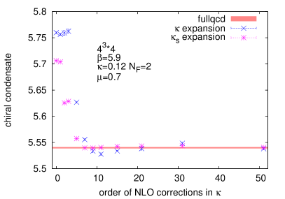
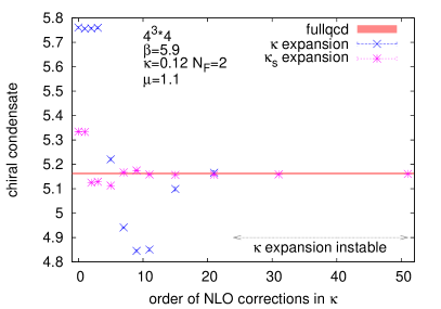
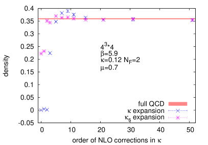
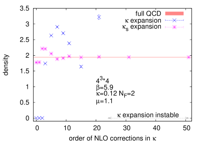
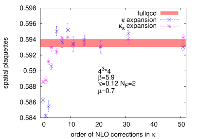
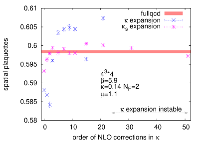
Figure 2: Convergence checks for the N^qLO $\kappa$- and $\kappa_{s}$-expansion on a $4^{4}$ lattice, $n_{f}=2$ at $\beta=5.9$, $\mu=0.7$ (left) and $\mu=1.1$ (right), vs $q$. Top: Chiral condensate at $\kappa=0.12$. Middle: baryonic density at $\kappa=0.12$. Bottom: spatial plaquette at $\kappa=0.12$ (left) and $0.14$ (right).

3.3 Baryonic density at ”low” temperature.

Here we work on lattices with $N_{s}\geq 10$ and $N_{\tau}=8,10,12,16$ at at $\beta=5.8$. Although we do not aim at physical results at this stage, we can get a rough idea of the physical parameters from the scale estimate obtained by gradient flow for HD-QCD in LO. This gives $l_{t}$ of approximately $1.12,1.40,1.68,2.24$ fm, hence temperatures of $\simeq\,180,\cdots,90$ MeV. The quarks are very heavy.

The low $\mu$ region can be scanned by RW in first NLO. The data in the Fig. 3 are obtained with $N_{s}=10$ . Due to the small aspect ratio we have finite spatial size effects. Here we show only the baryonic density, the Polyakov loop plots have a similar behaviour. For the density we show separately the contributions from straight and decorated Polyakov loops, but notice that this is an NLO calculation, therefore also the former are not the same as in a LO calculation.

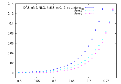
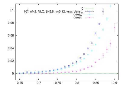
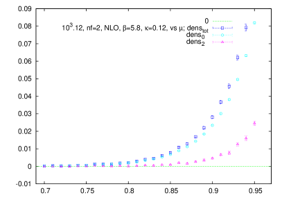
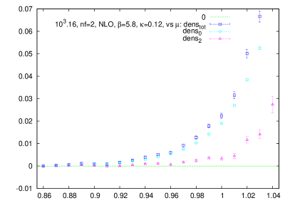
Figure 3: Baryon density from RW at $\beta=5,8$, $n_{f}=2$, NLO $\kappa=0.12$ Top: $T\sim 180$ and $145$ MeV. Bottom: $T\sim 120$ and $90$ MeV. Shown are also the contributions to the density from the straight and decorated Polyakov loops separately.

We observe a silver blaze region and an onset of the baryonic density at values of $\mu$ increasing with decreasing $T$. Notice that this is not the hadron-plasma transition which, at least in LO, takes place at much larger $\mu$ [16]. Moreover we notice a seizable structure at the onset which seems to indicate the presence of steps. It is tempting to see here a hint for a nuclear matter transition at a lower temperature, not attained yet in these simulations, but the effects of which would propagate in the phase diagram. Since the temperature favours the creation of charges the dependence of the onset on $T$ appears realistic.

The phase diagrams have been studied in LO in [16] by CLE and in NLO in [5] by RW. They show a very similar picture, with the transition line curving toward smaller $\mu$ with increasing temperature, to become very wide below a certain $\mu$-value. This indicates that the lower orders already catch the qualitative picture and also that at least in the region where they overlap both CLE and RW perform well. For further discussion and results see [5] and [16]. For further results from CLE see [6, 16, 17].

4 Summary

We here present a program to extend the HD-QCD to higher orders, approaching in this way QCD within a controlable, analytic approximation. This program appears feasible, at least for not too small (bare) quark masses. It is based on N^qLO CLE simulations at $\beta>5.7$ and for various $\mu$ and lattice sizes and $q$ significantly larger than 1. Note also that the analytic properties of the expansion and of the full process are different, therefore when the former converges onto the latter we have a good test that poles in the full drift are not quantitatively relevant and the results are error-free.

At $\mu$ below the hadron/plasma transition preliminary RW calculations in NLO indicate interesting effects at the onset of the baryonic density. The phase diagram has been drawn in lower orders both in CLE and RW exhibiting the $\beta,\mu$ dependence of the hadron-plasma transition. For further analysis and quantitative results we need, however, more statistics and data from CLE which are not restricted in $\mu$ and can go to larger $\kappa$ orders.

- [1] I. Bender, T. Hashimoto, F. Karsch, V. Linke, A. Nakamura, M. Plewnia, I.-O. Stamatescu, W. Wetzel, Nucl. Phys. Proc. Suppl. 26 (1992) 323
- [2] T. Blum, J.E. Hetrick, D. Toussaint, arxiv: hep-lat/9608127
- [3] J. Engels, O. Kaczmarek, F. Karsch, E. Laermann NPhProc 1999
- [4] G. Aarts, O. Kaczmarek, F. Karsch and I. -O. Stamatescu, Nucl. Phys. Proc. Suppl. 106 (2002) 456 [arXiv: hep-lat0110145]
- [5] R. De Pietri, A. Feo, E. Seiler, I.-O. Stamatescu, Phys. Rev. D 76 (2007) 114501 [arXiv:0705.3420]
- [6] G. Aarts, E.Seiler, D. Sexty and I.-O. Stamatescu, arXiv:1408.3770
- [7] J. Langelage, M. Neuman and O. Philipsen, arXiv:1403.4162 [hep-lat].
- [8] E. Seiler, D. Sexty and I.-O. Stamatescu, Phys. Lett. B 723 (2013) 213 [arxiv: 1211.3709]
- [9] M. Fromm, J. Langelage, S. Lottini, and O. Philipsen, JHEP 1201 (2012) 042 [arXiv:1111.4953]
- [10] G. Aarts, E. Seiler, I.-O. Stamatescu, Phys. Rev. D 81 (2010) 054508 [arXiv 0912.3360]
- [11] G. Aarts, F.A. James, E. Seiler, J.M. Pawlowski, D. Sexty, I.-O. Stamatescu, JHEP 1303 (2012) 073 [arXiv:1212:5231]
- [12] G. Aarts, L. Bongiovanni, E. Seiler, D. Sexty, I.-O. Stamatescu, Eur.Phys.J. A 49 (2013) 89, [arXiv:1303.6425]
- [13] A. Mollgaard and K. Splittorff, arXiv:1309.4335 (2013)
- [14] G. Aarts and I.-O. Stamatescu, JHEP 0809 (2008) 018 [arXiv:0807.1597]
- [15] D. Sexty, Phys. Lett. B 729 (2014) 108 [arXiv:1307.7748 [hep-lat]]
- [16] G. Aarts, F. Attanasio, B. Jäger, E. Seiler, D. Sexty, I.-O. Stamatescu, these proceedings
- [17] D. Sexty, these proceedings