Spurious harmonic response of multipulse quantum sensing sequences

Abstract

Multipulse sequences based on Carr-Purcell decoupling are frequently used for narrow-band signal detection in single spin magnetometry. We have analyzed the behavior of multipulse sensing sequences under real-world conditions, including finite pulse durations and the presence of detunings. We find that these non-idealities introduce harmonics to the filter function, allowing additional frequencies to pass the filter. In particular, we find that the XY family of sequences can generate signals at the $2f_{\mathrm{ac}}$, $4f_{\mathrm{ac}}$ and $8f_{\mathrm{ac}}$ harmonics and their odd subharmonics, where $f_{\mathrm{ac}}$ is the ac signal frequency. Consideration of the harmonic response is especially important for diamond-based nuclear spin sensing where the NMR frequency is used to identify the nuclear spin species, as it leads to ambiguities when several isotopes are present.

I. INTRODUCTION

Multipulse decoupling sequences, initially developed in the field of nuclear magnetic resonance (NMR) spectroscopy carr54 ; slichter , have enjoyed a renaissance for the control of individual quantum systems du09 ; ryan10 ; delange10 ; naydenov11 . The concept relies on periodic reversals of the coherent evolution of the system, where the effect of the environment is canceled over the complete sequence. Multipulse decoupling can be regarded as an efficient high-pass filter that averages out low frequency noise.

It has recently been recognized that decoupling sequences with equal pulse spacing offer an opportunity for sensitive ac signal detection delange11 ; zhao11 . By tuning the interpulse delay $\tau$, the sequence can be made commensurate with a signal’s periodicity leading to recoupling – that is, the decoupling fails for a specific set of signal frequencies that are an odd multiple of $1/(2\tau)$ (see Fig. 1a). The quantum system then effectively acts as a narrow-band lock-in amplifier kotler11 with demodulation frequency $f=k/(2\tau)$ and approximate bandwidth $f/(N/2)$, where $N$ is the total number of pulses in the sequence and $k=1,3,5,...$ is the resonance order. A precise transfer function of decoupling filters has been given in several recent papers cywinski08 ; kotler11 ; delange11 .

Multipulse sensing can greatly improve detection sensitivity, as it selectively measures the influence of a desired ac signal while suppressing unwanted noise. Moreover, the technique presents an opportunity to perform spectroscopy over a wide frequency range cywinski08 ; alvarez11 ; bylander11 ; gustavsson12 ; romach15 . A particularly important application has been the detection of nanoscale NMR signals using single spins in diamond where the nuclear Larmor frequency is taken as a fingerprint for the detected spin species taminiau12 ; zhao12 ; kolkowitz12 ; shi14 ; staudacher13 ; loretz14 ; muller14 ; devience15 ; rugar15 ; haberle15 ; loretz14science . Although mostly developed in the context of single spin magnetometry, multipulse sensing sequences have been applied to other quantum systems including trapped ions kotler11 and superconducting qubits bylander11 ; gustavsson12 .

In this paper we consider a specific class of multipulse sensing sequences known as the XY-family of sequences gullion90 . XY-type sequences use the common template of equidistant $\pi$ pulses, but pulse phases are judiciously alternated so as to cancel out pulse imperfections, such as pulse amplitude or detuning. The XY-family has become widely popular for measurements that require a large number of pulses $N$, and it has been the sequence of choice for most reported NV-based NMR experiments staudacher13 ; loretz14 ; muller14 ; devience15 ; rugar15 ; haberle15 ; loretz14science .

Here we show that the phase alternation of XY-type sequences causes additional frequencies to pass the multipulse filter. In particular, we show that an ac signal with frequency $f_{\mathrm{ac}}$ will produce response at the 2^nd , 4^th and 8^th harmonics (and their $k$’th subharmonics), depending on the sequence used. The harmonics are caused by a combination of time evolution during the finite duration of $\pi$ pulses and the “superperiods” introduced by phase cycling. Although the feature is generic to all experiments, it is most prominent for low pulse amplitudes, short interpulse delays, and if a static detuning is present. The feature is significant because it leads to further ambiguities in signal analysis and complicates interpretation of spectra.

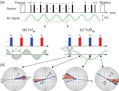
Figure 1: (a) Generic scheme of multipulse quantum sensing based on Carr-Purcell decoupling. The detection frequency $f=1/(2\tau)$ is adjusted to match the ac signal frequency $f_{\mathrm{ac}}$. (b,c) Sensor phase accumulation for the XY4 sequence for the fundamental signal $f=f_{\mathrm{ac}}$ and the 2^nd harmonic signal $f=2f_{\mathrm{ac}}$. Gray shaded areas show periods where phase accumulation occurs. (d) Bloch vector picture of the basic mechanism for phase accumulation at the 2^nd harmonic. ${\bf n_{1..4}}$ are rotation axes of $\pi$ pulses and $\theta_{\mathrm{eff}}$ is the angle of the effective field, as explained in the text.

II. THEORY

In order to understand the generation of harmonics we consider the simple case of an XY4 sequence exposed to an ac signal with frequency $f_{\mathrm{ac}}$. The basic building block of the XY4 sequence consists of four $\pi$ pulses with alternating $X$,$Y$ phases gullion90 (see Fig. 1b,c). In an ordinary sensing experiment, the interpulse spacing $\tau$ is matched to half the periodicity of the ac signal ($f=f_{\mathrm{ac}}$), leading to a constructive addition of phase during free evolution intervals. The phase accumulated per period $\tau$ is

$$\phi_{\mathrm{free}}=\frac{2\Omega\tau}{\pi}\ ,$$ (1)

and the phase accumulated during the entire sequence is $N\phi_{\mathrm{free}}$, where $\Omega$ is the amplitude of the ac signal. $\Omega$ represents a coupling constant with units of angular frequency.

In any realistic experimental implementation, $\pi$ pulses have a finite duration, and additional time evolution of the quantum system will occur pasini11 . For the example of the XY4 sequence, we find that a feature of the additional time evolution is phase accumulation at the second harmonic where $f=2f_{\mathrm{ac}}$. This phase accumulation is different from $\phi_{\mathrm{free}}$ in that it occurs during $\pi$ pulses, and not during free evolution intervals.

The feature can be understood by a picture of Bloch vector rotations (Fig. 1d). For simplicity, we assume that the ac field has maximum amplitude during $\pi_{X}$ pulses (and is zero during $\pi_{Y}$ pulses), and we neglect the free evolution during $\tau$. The action of the XY4 block can then be described by a set of four $\pi$-rotations $R_{\bf\hat{n}_{1...4}}^{\pi}$ around the axes

$${\bf\hat{n}_{1}} = (\cos\theta_{\mathrm{eff}},0,\sin\theta_{\mathrm{eff}})\ ,$$

$${\bf\hat{n}_{2}} = (0,1,0)\ ,$$

$${\bf\hat{n}_{3}} = (\cos\theta_{\mathrm{eff}},0,-\sin\theta_{\mathrm{eff}})\ ,$$

$${\bf\hat{n}_{4}} = (0,1,0)\ .$$ (2)

Axes ${\bf\hat{n}_{1}}$ and ${\bf\hat{n}_{3}}$ correspond to the $x$-axis tilted by the effective field angle $\theta_{\mathrm{eff}}=\tan^{-1}(\Omega/\omega_{1})\approx\Omega/\omega_{1}$ slichter , where $\omega_{1}$ is the angular velocity (Rabi frequency) of $\pi$ rotations. The key feature here is that ${\bf\hat{n}_{1}}\not\parallel{\bf\hat{n}_{3}}$ due to the change in sign of the ac signal. Assuming the Bloch vector is initially aligned with the $x$-axis, the vector orientation after the four $\pi$-rotations is

$$R_{\bf\hat{n}_{4}}^{\pi}R_{\bf\hat{n}_{3}}^{\pi}R_{\bf\hat{n}_{2}}^{\pi}R_{\bf\hat{n}_{1}}^{\pi}(1,0,0)=(\cos 4\theta_{\mathrm{eff}},0,-\sin 4\theta_{\mathrm{eff}})\ .$$ (3)

This corresponds to a net rotation around the $y$-axis by an angle $4\theta_{\mathrm{eff}}\approx 4\Omega/\omega_{1}$. The sensor therefore acquires an additional “anomalous” phase during the XY4 block, on average

$$\phi_{\pi}\approx\theta_{\mathrm{eff}}\approx\frac{\Omega}{\omega_{1}}=\frac{\Omega t_{\pi}}{\pi}$$ (4)

per $\pi$-pulse, where $t_{\pi}$ is duration of the square-shaped pulse. A similar calculation can be made for other harmonics and pulse sequences, and resulting phases have been collected in Table 1. These values are quantitative for the evolution during a single XY-block in the limit of weak coupling, but only qualitative for longer sequences (due to backaction) or if a detuning is present.

Harmonic	$2$	$4$	$8$	$2/3$	$4/3$	$8/3$
CPMG	—	—	—	—	—	—
XY4	$1.00\theta_{\mathrm{eff}}$	—	—	$1.00\theta_{\mathrm{eff}}$	—	—
XY8	$0.71\theta_{\mathrm{eff}}$	$0.27\theta_{\mathrm{eff}}$	—	$0.71\theta_{\mathrm{eff}}$	$0.65\theta_{\mathrm{eff}}$	—
XY16	$\ast$	$\ast$	$0.21\theta_{\mathrm{eff}}$	$\ast$	$\ast$	$0.91\theta_{\mathrm{eff}}$
	$2/5$	$4/5$	$8/5$	$2/7$	$4/7$	$8/7$
CPMG	—	—	—	—	—	—
XY4	$1.00\theta_{\mathrm{eff}}$	—	—	$1.00\theta_{\mathrm{eff}}$	—	—
XY8	$0.71\theta_{\mathrm{eff}}$	$0.65\theta_{\mathrm{eff}}$	—	$0.71\theta_{\mathrm{eff}}$	$0.27\theta_{\mathrm{eff}}$	—
XY16	$\ast$	$\ast$	$0.18\theta_{\mathrm{eff}}$	$\ast$	$\ast$	$0.32\theta_{\mathrm{eff}}$

Table 1: Anomalous phase $\phi_{\pi}$ at harmonics $f/f_{\mathrm{ac}}$ for CPMG, XY4, XY8 and XY16 sequences (see Ref. gullion90 for sequence definition). Values were determined by a numerical simulation as described in Section IV. $\theta_{\mathrm{eff}}\approx\Omega/\omega_{1}$ is the angle of the effective field. Entries marked by $\ast$ indicate that harmonics only appear in the presence of a static detuning.

The anomalous phase $\phi_{\pi}$ can be compared to the ordinary phase $\phi_{\mathrm{free}}$, providing a “relative strength” $r=\phi_{\pi}/\phi_{\mathrm{free}}$ of harmonics compared to the fundamental signal. For the example of the 2^nd harmonic in XY4 detection,

$$r=\frac{\phi_{\pi}}{\phi_{\mathrm{free}}}=\frac{t_{\pi}}{2\tau}\ .$$ (5)

Other harmonics and sequences follow by using the appropriate multiplier from Table 1. We find that the phase accumulated during $\pi$ rotations is equal to the phase accumulated during free evolution, scaled by $t_{\pi}/2\tau$. Since most often $t_{\pi}\ll\tau$, the harmonics will typically be much weaker than the fundamental signal. The harmonics may, however, become relevant if one intends to detect a weak ac signal in the presence of a strong, undesired signal. Note finally that higher order resonances ($k>1$) are not attenuated (sometimes enhanced) for anomalous signals, unlike the ordinary signals where $\phi_{\mathrm{free}}\propto 1/k$ taminiau12 .

III. SINGLE-SPIN MAGNETOMETRY

The above considerations apply to several relevant situations in single spin magnetometry of nanoscale NMR signals. Here, the precessing nuclear magnetization from single nuclei taminiau12 ; zhao12 ; kolkowitz12 ; loretz14science or nuclear ensembles staudacher13 ; loretz14 ; muller14 ; devience15 ; rugar15 ; haberle15 provides the ac signal. In the following we focus our attention on the specific case of an electron-nuclear two-spin system, where the electronic spin serves as the quantum sensor. The Hamiltonian of this system in a rotating frame of reference is

$$\hat{H}=\underbrace{\Delta_{z}\hat{S}_{z}}_{\mathrm{static}}+\underbrace{\omega_{1}\{x_{\mathrm{mod}}(t)\hat{S}_{x}+y_{\mathrm{mod}}(t)\hat{S}_{y}\}}_{\mathrm{control}}+\underbrace{a_{\perp}\hat{S}_{z}\hat{I}_{x}+\omega_{0}\hat{I}_{z}}_{\mathrm{ac\ signal}}$$ (6)

where we have grouped terms into static, control and ac contributions. $\Delta_{z}$ represents a static detuning of the electron spin $\hat{S}$ with respect to the rotating frame of reference, $x_{\mathrm{mod}}(t)$ and $y_{\mathrm{mod}}(t)$ represent the amplitude modulation of the multipulse decoupling sequence (with values between -1 and 1), $a_{\perp}$ represents the transverse coupling to the nuclear spin $\hat{I}$, and $\omega_{0}=\gamma_{n}B+a_{||}\hat{S}_{z}\approx\gamma_{n}B+a_{||}/2$ is the effective Larmor frequency of the nuclear spin composed of static bias field $B$ and parallel hyperfine field contribution $a_{||}$ (see supplementary material to Ref. loretz14science for a detailed discussion). $\gamma_{n}$ is the nuclear gyromagnetic ratio.

Returning to our generic expression for anomalous phase accumulation, Eq. (4), we can associate $\Omega\rightarrow a_{\perp}/2$ and $f_{\mathrm{ac}}\rightarrow\omega_{0}/(2\pi)$. For the case of a large nuclear spin ensemble with rms nuclear field $B_{\mathrm{ac}}^{\mathrm{rms}}$, one would associate $\Omega\rightarrow\gamma_{e}B_{\mathrm{ac}}^{\mathrm{rms}}/2$, where $\gamma_{e}$ is the electron gyromagnetic ratio.

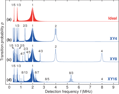
Figure 2: Simulated spectra showing response as a function of detection frequency $f=1/(2\tau)$ for coupling to a single nuclear spin with $f_{\mathrm{ac}}=\omega_{0}/(2\pi)=2\,\mathrm{MHz}$ and $\Omega=a_{\perp}/2=2\pi\cdot 200\,\mathrm{kHz}$. (a) Ideal sensing sequence with infinitely short $\pi$ pulses. Only the expected peaks at $f_{\mathrm{ac}}/k$ are observed. (b-d) Real XY4, XY8 and XY16 sequences gullion90 with finite, square-shaped $\pi$ pulses. Additional peaks at $2f_{\mathrm{ac}}/k$, $4f_{\mathrm{ac}}/k$ and $8f_{\mathrm{ac}}/k$ are observed, leading to a dense “forest” of peaks. Number of pulses was $N=480$, Rabi frequency was $\omega_{1}/2\pi=20\,\mathrm{MHz}$, and detuning (for c,d) was $\Delta_{z}=1\,\mathrm{MHz}$.

IV. SIMULATIONS

We have performed a set of numerical simulations loretz14science to investigate the time evolution of the Hamiltonian, Eq. (6). Our quantity of interest was the probability that the spin state at the end of the sequence $|\alpha\rangle$ deviated from its original state $|0\rangle$, expressed by the transition probability $p=1-|\langle\alpha|0\rangle|^{2}$.

Fig. 2 presents simulated spectra for different multipulse sensing sequences. The top panel shows the filter response for ideal $\pi$ rotations of infinitely short duration. As expected, signal peaks are generated at frequencies $f=f_{\mathrm{ac}}/k$, where $k=1,3,5,...$. Lower panels, by contrast, show the filter response of XY sequences for real $\pi$ rotations that have a finite duration. Many extra peaks appear corresponding to 2^nd , 4^th and 8^th harmonics of $f_{\mathrm{ac}}/k$. The spectra in Fig. 2 represent the response to a single ac signal (single spin) with frequency $f_{\mathrm{ac}}$. Obviously, if two or more signals were present, analysis of spectra would quickly become intractable.

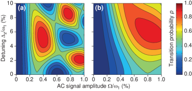
Figure 3: Simulated transition probability for the (a) 2^nd and (b) 4^th harmonic of the XY8 sequence. Horizontal axis is ac signal amplitude and vertical axis is detuning. Further simulation parameters were $N=1,024$ and $\omega_{1}/2\pi=20\,\mathrm{MHz}$.

Fig. 3 investigates the influence of a static detuning $\Delta_{z}$. Several effects may be noticed. First, a static detuning exacerbates the harmonic peaks – stronger anomalous response is generated for the same ac signal magnitude $\Omega$. Second, although not evident from this plot, peaks appear even at those harmonics where $\phi_{\pi}=0$ in Table 1. Third, the time evolution of $p$ becomes markedly different – values oscillate between $p=0...0.5$ in the absence of a detuning, whereas they can oscillate between $p=0...1$ and become aperiodic in the presence of a detuning.

V. EXPERIMENTS

We have experimentally verified the existence of harmonics using the nitrogen-vacancy (NV) center in diamond as the single spin sensor. The NV center is a prototype electron spin system ($S=1$) that can be optically detected at room temperature jelezko06 and that has served as a testbed for many recent multipulse sensing experiments. For our measurements, the NV center was polarized and read out using non-resonant green laser excitation, and manipulated using microwave control pulses with adjustable phase and amplitude loretz14 . A static bias field was applied to lift the spin degeneracy and all sensing experiments were carried out on the $m_{S}=0\leftrightarrow m_{S}=-1$ subsystem.

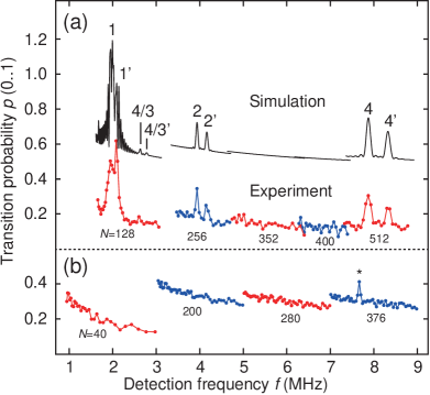
Figure 4: (a) Spectrum recorded by an NV center with two weakly coupled ¹³C nuclei, measured using an XY8 sequence. Multiple harmonics are clearly observed. Colors represent different datasets. Coupling constants for the two ¹³C were $a_{\perp}/2\pi=220\,\mathrm{kHz}$ and $a_{\perp}^{\prime}/2\pi=180\,\mathrm{kHz}$. The number of pulses $N$ is given in the plot. The associated total evolution time was $T=N/(2f)$. Further parameters were $\omega_{1}/2\pi=28\,\mathrm{MHz}$ and $\Delta_{z}=1.5\,\mathrm{MHz}$ (due to the ¹⁵N hyperfine splitting). (b) For comparison, spectrum recorded by an NV center with no ¹³C nearby. Peak marked by $\ast$ is due to an ensemble of ¹H with $B_{\mathrm{ac}}^{\mathrm{rms}}=400\,\mathrm{nT}$.

In a first experiment we have recorded the XY8 response of an NV center with two proximal ¹³C nuclei ($I=1/2$) in a bias field of $183\,\mathrm{mT}$. The nuclear Larmor frequencies of the two ¹³C nuclei in this field were $f_{\mathrm{ac}}=1.97\,\mathrm{MHz}$ and $f_{\mathrm{ac}}^{\prime}=2.08\,\mathrm{MHz}$. (The frequencies were slightly different due to a small parallel hyperfine contribution.) Fig. 4 shows the spectral response over the frequency range of $f=1.5-9\,\mathrm{MHz}$. We found that almost all harmonics in that range could be resolved and matched with simulations using a single set of parameters.

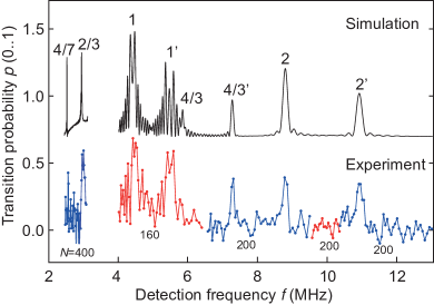
Figure 5: Spectrum recorded by an NV center coupled to its own ¹⁴N nucleus, measured using an XY8 sequence. Common coupling constant was $a_{\perp}/2\pi=280\,\mathrm{kHz}$. This coupling was due to a deliberate misalignment of the bias field of $\sim 8^{\circ}$ with respect to the NV symmetry axis. Further experimental parameters were similar to Fig. 4.

Fig. 5 shows a second example where the NV center’s electron spin was coupled to its own ¹⁴N nucleus ($I=1$). The ¹⁴N has two nuclear spin transitions, resulting in two signals with frequencies $f_{\mathrm{ac}}=4.4\,\mathrm{MHz}$ and $f_{\mathrm{ac}}^{\prime}=5.4\,\mathrm{MHz}$. Again, most expected harmonics could be observed and matched with simulations.

VI. AMBIGUITIES BETWEEN NMR SIGNALS

The feature of harmonics is of particular significance for recent nanoscale NMR experiments with near-surface NV centers. These experiments used spectral identification to discriminate different nuclear isotopes in samples by their NMR frequencies, most prominently ¹H , ¹³C , ¹⁹F , ²⁹Si and ³¹P staudacher13 ; loretz14 ; muller14 ; devience15 ; rugar15 ; haberle15 .

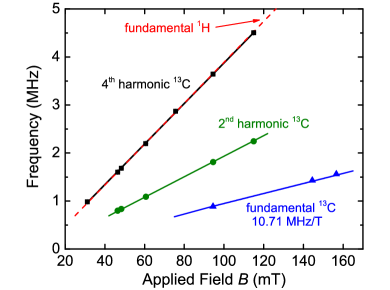
Figure 6: Frequency of peak response for various magnetic bias fields $B$, measured using an XY8 sequence. Points are measured peak positions. Solid lines have slopes chosen to be $1\times$, $2\times$ and 4$\times$ the gyromagnetic ratio of ¹³C . The red dashed line has slope given by the gyromagnetic ratio of ¹H , and is almost identical to the ¹³C 4^th harmonic line (black line).

We now show that in the presence of more than one nuclear species, harmonics can produce coincidential overlap between signals and lead to ambiguities in peak assignments. As a particular example we consider the detection of a weak ¹H signal in the presence of ¹³C , which is a situation typical to NV centers in natural abundance diamond substrates ($\sim 1$% ¹³C content) loretz14science . Here the signal overlap arises because the ¹H NMR frequency coincides with the $4\times$ harmonic of ¹³C to within 0.6%. We find that single ¹³C nuclei can generate signatures virtually identical to those of single ¹H , including a Zeeman scaling with magnetic field and a quantum-coherent oscillation of the signal.

We begin with the scaling of the peak frequency with bias field $B$, as shown in Fig. 6. The measured peak positions (points) can all be associated with the response from a single ¹³C nucleus at either its fundamental Larmor frequency, or its 2^nd or 4^th harmonic. The linear slope of the fundamental frequency (blue line) is given by the gyromagnetic ratio of ¹³C ($\gamma_{n}=10.71\,\mathrm{MHz/T}$) and is indicative of the nuclear species, while the slopes of the two harmonic frequencies are enhanced with apparent gyromagnetic ratios of $2\gamma_{n}$ and $4\gamma_{n}$. Since the value of $4\gamma_{n}=42.82\,\mathrm{MHz/T}$ coincides with the gyromagnetic ratio of protons ($\gamma_{n}=42.57\,\mathrm{MHz/T}$) within experimental uncertainty, the nuclear isotope cannot be uniquely identified.

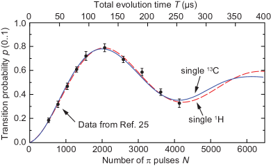
Figure 7: Peak transition probability with increasing total evolution time $T=N\tau$ measured at the expected ¹H resonance. Black data points are taken from Ref. loretz14science . Red dashed curve shows simulation for a single ¹H spin with coupling constant $a_{\perp}/2\pi=14\,\mathrm{kHz}$. Blue solid curve shows simulation for the 4^th harmonic of a single ¹³C spin with a coupling constant $a_{\perp}/2\pi=150\,\mathrm{kHz}$. Pulse sequence was XY8. Further parameters were $B=182\,\mathrm{mT}$, $\omega_{1}/2\pi=25\,\mathrm{MHz}$ and $\tau=61.5\,\mathrm{ns}$.

Isotope	Frequency	Mimicking	Harmonic	Harmonic	Rel. freq.
		isotope		frequency	difference
1H	4.257 MHz	13C	$4\times$	4.282 MHz	0.6%
2H	0.654 MHz	1H	$2/13\times$	0.655 MHz	0.2%
29Si	0.846 MHz	1H	$1/5\times^{\ast}$	0.851 MHz	0.7%
		13C	$4/5\times$	0.856 MHz	1.2%
31P	1.723 MHz	1H	$2/5\times$	1.703 MHz	1.2%

Table 2: Examples of coincidential overlap between fundamental and harmonic frequencies for important NMR isotopes. Values are given for a $100\,\mathrm{mT}$ bias field. All above harmonics are visible in Fig. 2. ^∗Ordinary (not anomalous) harmonic.

We found also the time evolutions of fundamental and harmonic signals produce indistinguishable signatures. Fig. 7 shows the peak height of an apparent proton signal as the number of pulses $N$ in increased. An oscillating signal is observed that can be reproduced by either of two simulations, one assuming the presence of a single ¹H and one of a single ¹³C . Again, no conclusion can be made on the identity of the nuclear species.

The above example illustrates that assignment of a signal based on a single peak is in general insufficient. A more trustworthy identification could be obtained by measuring a wide spectral region containing several harmonics, as shown in Fig. 4. For the specific situation of ¹³C and ¹H , the second harmonic at twice the ¹³C Larmor frequency (roughly half the ¹H frequency) could serve as a tell-tale signature of ¹³C . This peak is absent for ¹H .

We note that the ambiguity between ¹H and ¹³C is just one particular case. Given the large number of harmonics and nuclear isotopes, many other pairs of nuclear species with potential overlap can be expected. Table 2 collects a few additional cases of particular relevance to NMR where such coincidential signal overlap could occur. Consideration of harmonics is especially important in the presence of ¹H or for ¹³C -containing diamond, because these species often produce a relatively strong signal.

VII. SUMMARY

In summary, we have investigated the spectral filtering characteristics of an important class of multipulse quantum sensing sequences, the XY-family of sequences. We found the time evolution during finite $\pi$ pulses, which is present in any experimental implementation, to cause phase build-up at higher harmonics of the signal frequency, leading to sets of additional peaks in the spectrum. We have further investigated this feature by simulations and experiments of single NV centers in diamond. The feature has particular significance for nanoscale NMR experiments that rely on spectral identification. Specifically, we found that signal detection at a single frequency is in general insufficient to uniquely assign a certain nuclear spin species.

We finally mention several sensing schemes that do not suffer from the ambiguities inherent to multipulse sequences. Namely these include rotating-frame spectroscopy yan13 ; loretz13 ; london13 and free precession techniques mamin13 ; laraoui13 ; taminiau14 . Moreover, it may be possible to craft varieties of sequences that avoid harmonic resonances yet maintain superior static error compensation, such as sequences with composite $\pi$ pulses ryan10 ; souza11 , locally non-uniform pulse spacing zhao14 , or aperiodic phase alternation. Although the alternative schemes have their own restrictions and may not always be available, they could offer independent verification of spectral features.

ACKNOWLEDGMENTS

This work was supported by Swiss NSF Project Grant $200021\_137520$, the NCCR QSIT, the DIADEMS programme of the European Commission, and the DARPA QuASAR program.

References

- (1) H. Y. Carr, and E. M. Purcell, Effects of Diffusion on Free Precession in Nuclear Magnetic Resonance Experiments Phys. Rev. 94, 630 (1954).
- (2) C. P. Slichter, C. P. Slichter, Principles of Magnetic Resonance, (Springer, Heidelberg, 1996).
- (3) J. Du et al., Preserving electron spin coherence in solids by optimal dynamical decoupling, Nature 461, 1265-1268 (2009).
- (4) C. A. Ryan, J. S. Hodges, and D. G. Cory, Robust decoupling techniques to extend quantum coherence in diamond, Phys. Rev. Lett. 105, 200402 (2010).
- (5) G. de Lange, Z. Wang, D. Riste, V. Dobrovitski, and R. Hanson, Universal dynamical decoupling of a single solid-state spin from a spin bath, Science 330, 60-63 (2010).
- (6) B. Naydenov et al., Dynamical decoupling of a single-electron spin at room temperature, Phys. Rev. B 83, 081201 (2011).
- (7) G. De Lange, D. Riste, V. V. Dobrovitski, and R. Hanson, Single-spin magnetometry with multipulse sensing sequences, Phys. Rev. Lett. 106, 080802 (2011).
- (8) N. Zhao, J. L. Hu, S. W. Ho, J. T. K. Wan, and R. B. Liu, Atomic-scale magnetometry of distant nuclear spin clusters via nitrogen-vacancy spin in diamond, Nature Nanotech. 6, 242-246 (2011).
- (9) S. Kotler, N. Akerman, Y. Glickman, A. Keselman, and R. Ozeri, Single-ion quantum lock-in amplifier, Nature 473, 61-65 (2011).
- (10) L. Cywinski, R. M. Lutchyn, C. P. Nave, and S. Das Sarma, How to enhance dephasing time in superconducting qubits, Phys. Rev. B 77, 174509 (2008).
- (11) G. A. Alvarez, and D. Suter, Measuring the spectrum of colored noise by dynamical decoupling, Phys. Rev. Lett. 107, 230501 (2011).
- (12) J. Bylander et al., Noise spectroscopy through dynamical decoupling with a superconducting flux qubit, Nature Phys. 7, 565-570 (2011).
- (13) S. Gustavsson et al., Dynamical decoupling and dephasing in interacting two-level systems, Phys. Rev. Lett. 109, 010502 (2012).
- (14) Y. Romach et al., Spectroscopy of surface-induced noise using shallow spins in diamond, Phys. Rev. Lett. 114, 017601 (2015).
- (15) T. H. Taminiau et al., Detection and control of individual nuclear spins using a weakly coupled electron spin, Phys. Rev. Lett. 109, 137602 (2012).
- (16) N. Zhao et al., Sensing single remote nuclear spins, Nature Nanotech. 7, 657 (2012).
- (17) S. Kolkowitz, Q. P. Unterreithmeier, S. D. Bennett, and M. D. Lukin, Sensing distant nuclear spins with a single electron spin, Phys. Rev. Lett. 109, 137601 (2012).
- (18) F. Shi et al., Sensing and atomic-scale structure analysis of single nuclear-spin clusters in diamond, Nat. Phys. 10, 21-25 (2014).
- (19) T. Staudacher et al., Nuclear magnetic resonance spectroscopy on a (5-nanometer)3 sample volume, Science 339, 561-563 (2013).
- (20) M. Loretz, S. Pezzagna, J. Meijer, and C. L. Degen, Nanoscale nuclear magnetic resonance with a 1.9-nm-deep nitrogen-vacancy sensor, Appl. Phys. Lett. 104, 33102 (2014).
- (21) C. Muller et al., Nuclear magnetic resonance spectroscopy with single spin sensitivity, Nature Commun. 5, 4703-4703 (2014).
- (22) S. J. Devience et al., Nanoscale NMR spectroscopy and imaging of multiple nuclear species, Nature Nanotech. 10, 129-134 (2015).
- (23) D. Rugar et al., Proton magnetic resonance imaging using a nitrogen–vacancy spin sensor, Nature Nanotech. 10, 120-124 (2015).
- (24) T. Haberle, D. Schmid-Lorch, F. Reinhard, and J. Wrachtrup, Nanoscale nuclear magnetic imaging with chemical contrast, Nature Nanotech. 10, 125-128 (2015).
- (25) M. Loretz et al., Single-proton spin detection by diamond magnetometry, Science 10.1126/science.1259464 (2014); published online 16 October 2014.
- (26) T. Gullion, D. B. Baker, and M. S. Conradi, New, compensated Carr-Purcell sequences, J. Magn. Res. 89, 479-484 (1990).
- (27) S. Pasini, P. Karbach, and G. S. Uhrig, High-order coherent control sequences of finite-width pulses, Europhys. Lett. 96, 10003 (2011).
- (28) F. Jelezko, and J. Wrachtrup, Single defect centres in diamond: A review, phys. stat. sol. (a) 203, 3207 (2006).
- (29) F. Yan et al., Rotating-frame relaxation as a noise spectrum analyser of a superconducting qubit undergoing driven evolution, Nature Commun. 4, 2337 (2013).
- (30) M. Loretz, T. Rosskopf, and C. L. Degen, Radio-frequency magnetometry using a single electron spin, Phys. Rev. Lett. 110, 017602 (2013).
- (31) P. London et al., Detecting and polarizing nuclear spins with double resonance on a single electron spin, Phys. Rev. Lett. 111, 067601 (2013).
- (32) H. J. Mamin et al., Nanoscale nuclear magnetic resonance with a nitrogen-vacancy spin sensor, Science 339, 557-560 (2013).
- (33) A. Laraoui et al., High-resolution correlation spectroscopy of C-13 spins near a nitrogen-vacancy centre in diamond, Nature Commun. 4, 1651 (2013).
- (34) T. H. Taminiau, J. Cramer, T. van der Sar, V. V. Dobrovitski, and R. Hanson, Universal control and error correction in multi-qubit spin registers in diamond, Nature Nanotech. 9 (2014).
- (35) A. M. Souza, G. A. Alvarez, and D. Suter, Robust dynamical decoupling for quantum computing and quantum memory, Phys. Rev. Lett. 106, 240501 (2011).
- (36) N. Zhao, J. Wrachtrup, and R. B. Liu, Dynamical decoupling design for identifying weakly coupled nuclear spins in a bath, Phys. Rev. A 90, 032319 (2014).