Time-dependent thermal transport theory

Abstract

Understanding thermal transport in nanoscale systems presents important challenges to both theory and experiment. In particular, the concept of local temperature at the nanoscale appears difficult to justify. Here, we propose a theoretical approach where we replace the temperature gradient with controllable external black-body radiations. The theory recovers known physical results, for example the linear relation between the thermal current and the temperatures difference of two black-bodies. Furthermore, our theory is not limited to the linear regime and goes beyond accounting for non linear effects and transient phenomena. Since the present theory is general and can be adapted to describe both electron and phonon dynamics, it provides a first step towards a unified formalism for investigating thermal and electronic transport.

The wide research field of energy transport in nanoscale systems is very active: groundbreaking advances in understanding the physics of this important phenomenon have been made in recent years Volz (2009); Dubi and Di Ventra (2011); Li et al. (2012), e.g., the measurement of the quantum of thermal conductance Rego and Kirczenow (1998); Schwab et al. (2000), thermal quantum rectifiers Zhu et al. (2014), breaking of the Fourier’s law Dubi and Di Ventra (2011). Over time, different theoretical approaches have been proposed ranging from the Landauer’s theory of electrical and thermal transport Di Ventra (2008); Volz (2009); Nolas et al. (2001); Chen (2005); Guedon et al. (2012), molecular dynamics Lee et al. (2007), quantum and classical Boltzmann equation Cahill et al. (2003), non-equilibrium Green’s function formalisms Galperin et al. (2007); Wang et al. (2008); Saha et al. (2011); Stefanucci and van Leeuwen (2013); Sánchez and López (2013); López and Sánchez (2013), to the theory of open quantum systems Gardiner and Zoller (2000); Breuer and Petruccione (2002); Biele and D’Agosta (2012); Biele et al. (2014) to point out just a few. This activity is justified by the range of possible applications from thermoelectric energy conversion, heat dissipation, kinetics of chemical reactions, to a very new and more fundamental definition of thermodynamical equilibrium Nolas et al. (2001); Ponomarev et al. (2011); Volz (2009), to name just a few. It is a common everyday experience that two macroscopic bodies in contact with each other equilibrate in the long-time limit to the same temperature. Microscopically, equilibration means that there is not a net energy flow between the two bodies but energy exchanges, in form of small fluctuations, are still present. Since the direction of the energy flow is determined by the sign of the difference between the temperatures of the bodies, we conclude that the absence of an energy flow implies the two bodies have the same temperature. This law of thermodynamics provides an operative definition of the temperature difference. What makes thermal transport at the nanoscale a difficult theoretical problem is that the very basic fundamentals of standard thermodynamics cannot be applied, and the idea of thermalization needs revisiting. In the past, attempts have been made to introduce a position dependent temperature Zubarev (1994), but they do not provide a satisfactory definition of local temperature. Indeed, the concepts of local Hamiltonian, useful to define a local energy density, local thermal current, and local nano-scale thermal gradient are not uniquely defined. Recently, a way out, restricted to small thermal gradients, has been put forward using an effective gravitational field, as originally proposed by Luttinger Luttinger (1964), that mimics the effect of the temperature gradient Eich et al. (2014a, b). Here, we propose an alternative approach where the temperature field is established by two or more blackbodies of known thermal properties. Besides thermal transport at the nano-scale, this theory can be used to understand energy transport in cold atoms, biological or optical systems. We first lay down the basic formalism and then consider a simple one-electron model system. However, our theory can be combined with the general framework of time-dependent current-density functional theory (TDCDFT) Marques et al. (2006); Ullrich (2012); Giuliani and Vignale (2005) to consider also many-body systems. More important, our approach is not restricted to the linear response or weak coupling regimes, and we can easily investigate the interesting cases of both strong coupling - recovering the Kramers’ turnover Hänggi and Borkovec (1990) - and large temperature gradients. Finally, we have access to the full dynamics of the system, therefore we can investigate transient regimes, usually unaccessible to other formalisms. Last but not least, our theory can be applied to investigating the phonon thermal transport. In this respect, it could be seen as a first step towards a unified ab-initio formalism for thermal and electric transport.

A blackbody, according to its original definition Kirchhoff (1860), is a macroscopic object that absorbs all the radiation impinging on it, and in thermal equilibrium it emits electromagnetic radiation according to the Planck’s law, whose spectrum is determined solely by the temperature of the blackbody and not by its shape or composition Planck (1901, 1900). If we connect a blackbody with a cavity made of perfect reflecting walls, the radiation inside the cavity thermally equilibrates with the blackbody radiation, and any object in this cavity will also thermalize. By changing the temperature of the blackbody we control both the temperature inside the cavity and that of the body. When thermal equilibrium is reached, at any point in the cavity the electromagnetic radiation follows Planck’s law with the temperature of the blackbody. Ultimately we can extract the local temperature from the observation of the energy radiation and this serves us in the following to construct a formalism for thermal transport. Our thermometer, or thermal source, is indeed a blackbody which radiates according to its temperature.

To begin with, we consider an electronic system coupled to any strength to the black-body radiation and weakly to the free field of an external environment. The dynamics of the black-body radiation is determined solely by the blackbody itself. Here, we assume the macroscopic parameters of the blackbody to be constant in time and treated classically. At the same time, to allow for relaxation and to mimic the experimental set-ups, the system is embedded in a bosonic environment, kept at constant temperature $T_{E}$, with which the system can exchange energy via spontaneous and stimulated emission or absorption. The total Hamiltonian where we treat the environment quantum-mechanically (we set $\hbar=e=m=1/(4\pi\epsilon_{0})=1$), is

$$\hat{H}_{T}=\sum_{i=1}^{N}\left[\frac{\left(\hat{\mathbb{p}}_{i}-\hat{\mathbb{A}}_{F}(\hat{\mathbb{r}}_{i})-{\mathbb{A}}_{\mathrm{BB}}(\hat{\mathbb{r}}_{i},t)\right)^{2}}{2}+U(\hat{\mathbb{r}}_{i},t)\right]+\hat{H}_{F},$$ (1)

where $\hat{H}_{F}=\sum_{\mathbb{k},s}\omega_{\mathbb{k}}\hat{b}^{\dagger}_{\mathbb{k},s}\hat{b}_{\mathbb{k},s}$ is the Hamiltonian of the free field of the environment and $\hat{\mathbb{A}}_{F}$ its corresponding vector potential. In addition, $U$ is an external potential and ${\mathbb{A}}_{\mathrm{BB}}$ describes the electromagnetic radiation emitted by the blackbody sources. We neglect the direct interaction of the free field with the black-body radiation. This can be justified by observing that the photon-photon interaction is small, consequently the contributions of the terms where, e.g., a photon from the blackbody scatters with the free field and then is absorbed by the system, are negligible. Therefore, we write $\hat{H}_{T}=\hat{H}_{S}(t)+\hat{I}_{S,F}+\hat{H}_{F}$ where we have included the system-blackbody interaction in the system Hamiltonian, $\hat{H}_{S}=\sum_{i=1}^{N}\left(\hat{\mathbb{p}}^{2}_{i}/2+U(\mathbb{r}_{i},t)-{\mathbb{A}}_{\mathrm{BB}}(\mathbb{r}_{i},t)\cdot\hat{\mathbb{p}}_{i}\right)$, and the quadratic term ${\mathbb{A}}_{\mathrm{BB}}^{2}$ in the external potential $U$. The free vector-field is written as $\hat{\mathbb{A}}_{F}(\mathbb{r})=\sum_{\mathbb{k},s}p_{\mathbb{k},s}\left(\hat{b}_{\mathbb{k},s}\exp(i\mathbb{k}\mathbb{r})+\hat{b}^{\dagger}_{\mathbb{k},s}\exp(-i\mathbb{k}\mathbb{r})\right)\mathbb{\epsilon}_{\mathbb{k},s}$, where $p_{k}=\sqrt{2\pi/(\omega_{k}V)}$ and $\hat{b}_{\mathbb{k}}^{\dagger}$ is the creation operator for a free-field mode with polarization direction $\mathbb{\epsilon}_{\mathbb{k},s}$. Finally, by exploiting the field expansion $\hat{\Psi}=\sum_{\alpha}\hat{c}_{\alpha}(t)\phi_{\alpha}(r)$, the system-environment interaction can be written, in the Coulomb gauge as $\hat{I}_{S,F}=\sum_{\alpha,\beta,\mathbb{k},s}g_{\alpha\beta,\mathbb{k},s}\>\hat{c}_{\alpha}^{\dagger}\hat{c}_{\beta}\left(\hat{b}_{\mathbb{k},s}+\hat{b}_{\mathbb{k},s}^{\dagger}\right)$, where we have defined, $g_{\alpha\beta,\mathbb{k},s}=ip_{\mathbb{k}}\int\mathrm{d}V\phi_{\alpha}^{*}(\mathbb{r})\mathbb{\epsilon}_{\mathbb{k},s}\cdot\mathbb{\nabla}\phi_{\beta}(\mathbb{r})$. Here, we have assumed that the system size is small in comparison to the wavelengths of the electromagnetic field (dipole approximation) . Furthermore, the operators $\hat{c}^{\dagger}_{\alpha}$ create the $\alpha$’s energy eigenstate of the initial Hamiltonian $H_{S}(0)$. These energy eigenstates will serve as a natural basis set for our following considerations. Naturally, the (local) density of states associated with the eigenstates of this Hamiltonian defines how efficient the coupling between the system and the black-body radiations is Stefanucci and van Leeuwen (2013); Di Ventra (2008).

As we are interested only in the system dynamics, we will examine the dynamics of the expectation value of the one-particle density operator $f_{\alpha\beta}=\langle\hat{c}^{\dagger}_{\alpha}\hat{c}_{\beta}\rangle$, easily derived from the equation of motion for $\hat{c}^{\dagger}_{\alpha}\hat{c}_{\beta}$, $i\partial_{t}f_{\alpha\beta}=\langle[\hat{H}_{S}(t),\hat{c}^{\dagger}_{\alpha}\hat{c}_{\beta}]\rangle+\sum_{\gamma,\mathbb{k}}[g_{\beta,\gamma,\mathbb{k}}(\langle\hat{b}_{\mathbb{k}}\hat{c}^{\dagger}_{\alpha}\hat{c}_{\gamma}\rangle+\langle\hat{b}^{\dagger}_{\mathbb{k}}\hat{c}^{\dagger}_{\alpha}\hat{c}_{\gamma}\rangle)-g_{\gamma,\alpha,\mathbb{k}}(\langle\hat{b}_{\mathbb{k}}\hat{c}^{\dagger}_{\gamma}\hat{c}_{\beta}\rangle+\langle\hat{b}^{\dagger}_{\mathbb{k}}\hat{c}^{\dagger}_{\gamma}\hat{c}_{\beta}\rangle)]$, where we included the spin index $s$ in the components of $\mathbb{k}$. Its solution requires the knowledge of the dynamics of $\hat{b}_{\mathbb{k}}\hat{c}^{\dagger}_{\alpha}\hat{c}_{\beta}$,

$$i\partial_{t}\hat{b}_{\mathbb{k}}\hat{c}^{\dagger}_{\alpha}\hat{c}_{\beta} = \left[\hat{H}_{S},\hat{b}_{\mathbb{k}}\hat{c}^{\dagger}_{\alpha}\hat{c}_{\beta}\right]+\omega_{\mathbb{k}}\hat{b}_{\mathbb{k}}\hat{c}^{\dagger}_{\alpha}\hat{c}_{\beta}$$

$$+\sum_{\gamma,\delta,\mathbb{l}}g_{\gamma\delta,\mathbb{l}}\left[\hat{c}^{\dagger}_{\alpha}\hat{c}_{\beta}\hat{c}^{\dagger}_{\gamma}\hat{c}_{\delta}\delta_{\mathbb{k},\mathbb{l}}\right.$$

$$+\left.\left\{\hat{b}_{\mathbb{k}}(\hat{b}_{\mathbb{l}}+\hat{b}^{\dagger}_{\mathbb{l}})-\delta_{\mathbb{k},\mathbb{l}}\right\}\left(\hat{c}^{\dagger}_{\alpha}\hat{c}_{\delta}\delta_{\gamma\beta}-\hat{c}^{\dagger}_{\gamma}\hat{c}_{\beta}\delta_{\delta\alpha}\right)\right].$$

A similar equation holds for $\hat{b}^{\dagger}_{\mathbb{k}}\hat{c}^{\dagger}_{\alpha}\hat{c}_{\beta}$. These equations of motion are not in a closed form, and any attempt to solve them by investigating the dynamics of the operators appearing on the right hand side leads to an infinite hierarchy of equations. For this reason, we decouple the dynamics of the system and the field, i.e., we assume that $\langle\hat{b}_{\mathbb{k}}\hat{b}^{\dagger}_{\mathbb{l}}\hat{c}^{\dagger}_{\alpha}\hat{c}_{\beta}\rangle\approx\langle\hat{b}_{\mathbb{k}}\hat{b}^{\dagger}_{\mathbb{l}}\rangle\langle\hat{c}^{\dagger}_{\alpha}\hat{c}_{\beta}\rangle.$ With this approximation Eq. (Time-dependent thermal transport theory) is solved with a standard integration technique. Furthermore, by using that the initial-state correlation vanishes, $\langle\hat{b}^{\dagger}_{\mathbb{k}}\hat{c}^{\dagger}_{\alpha}\hat{c}_{\beta}\rangle(0)=\langle\hat{b}_{\mathbb{k}}\hat{c}^{\dagger}_{\alpha}\hat{c}_{\beta}\rangle(0)=0$ and that the environment is in thermal equilibrium, $n(\omega_{\mathbb{k}},T_{E})=\sum_{\mathbb{l}}\langle\hat{b}_{\mathbb{k}}(\hat{b}_{\mathbb{l}}+\hat{b}^{\dagger}_{\mathbb{l}})-\delta_{\mathbb{k},\mathbb{l}}\rangle$, where $n(\omega,T)$ is the Planck’s distribution at energy $\omega$ and temperature $T$, we arrive at a non-Markovian master equation

$$\begin{split}i\partial_{t}f_{\alpha\beta}=&\left\langle\left[\hat{f},\hat{H}_{S}\right]\right\rangle_{\alpha\beta}\\ &+i\sum_{\mathbb{k},\mathbb{l}}\int_{t_{0}}^{t}\mathrm{d}\tau\>C_{\mathbb{k},\mathbb{l}}(\tau,t)\left\langle\left[\hat{U}(\tau,t)\hat{f}(\tau)\hat{V}_{\mathbb{l}}\hat{U}^{\dagger}(\tau,t)\hat{V}_{\mathbb{k}}\right.\right.\\ &-\hat{U}(\tau,t)\hat{V}_{\mathbb{l}}\hat{f}(\tau)\hat{U}^{\dagger}(\tau,t)\hat{V}_{\mathbb{k}}\\ &-\hat{V}_{\mathbb{k}}\hat{U}(\tau,t)\hat{f}(\tau)\hat{V}_{\mathbb{l}}\hat{U}^{\dagger}(\tau,t)\\ &\left.\left.+\hat{V}_{\mathbb{k}}\hat{U}(\tau,t)\hat{V}_{\mathbb{l}}\hat{f}(\tau)\hat{U}^{\dagger}(\tau,t)\right]\right\rangle_{\alpha\beta}\\ &-2\int_{t_{0}}^{t}\mathrm{d}\tau\sum_{\begin{subarray}{c}\gamma,\delta,\sigma,\zeta\mathbb{k},\mathbb{l}\end{subarray}}V^{*}_{\delta\gamma,\mathbb{k}}V^{*}_{\sigma\zeta,\mathbb{l}}\sin(\omega_{\mathbb{k}}(t-\tau))\\ &\times\{\delta_{\beta\gamma}U_{\delta\alpha}(\tau,t)\langle\hat{c}^{\dagger}_{\alpha}\hat{c}_{\delta}\hat{c}^{\dagger}_{\sigma}\hat{c}_{\zeta}\rangle(\tau)\\ &-\delta_{\delta\alpha}U_{\beta\gamma}(\tau,t)\langle\hat{c}^{\dagger}_{\gamma}\hat{c}_{\beta}\hat{c}^{\dagger}_{\sigma}\hat{c}_{\zeta}\rangle(\tau)\}.\end{split}$$ (3)

Here, we have introduced the bath correlation function $C_{\mathbb{k},\mathbb{l}}(\tau,t)=\langle\{\hat{b}_{\mathbb{k}}(\tau)+\hat{b}^{\dagger}_{\mathbb{k}}(\tau)\}\{\hat{b}_{\mathbb{l}}(t)+\hat{b}^{\dagger}_{\mathbb{l}}(t)\}\rangle=(n(\omega_{\mathbb{k}},T)+1)e^{-i\omega_{\mathbb{k}}(\tau-t)}+n(\omega_{\mathbb{k}},T)e^{i\omega_{\mathbb{k}}(\tau-t)}$, and defined $V^{*}_{\beta\alpha,\mathbb{k}}=-ig_{\alpha\beta,\mathbb{k}}$ and $\hat{U}(\tau,t)=\hat{T}_{+}e^{-i\int_{\tau}^{t}\mathrm{d}t^{\prime}\hat{H}_{S}(t^{\prime})}$, where $\hat{T}_{+}$ is the time-ordering operator. The former equation describes a system under the influence of a classical black-body radiation, where the system can dissipate to or gain energy from the environment. It is known that for the system described by this master equation the detailed balance of the power spectrum of the correlation function $C_{k,l}(\omega)=\int_{-\infty}^{\infty}\exp(-i\omega(t-\tau))C_{k,l}(t,\tau)dt$, is the minimum requirement to reach thermal equilibrium with the free field. One can easily check that the detailed balance condition is satisfied by our correlation function. Then, without any external sources, the system evolving according to Eq. (3) reaches thermal equilibrium with the free field radiation. On the other hand, when external sources or driving potentials are present, the system does not reach any thermal equilibrium in general. However, we expect the system to reach a steady state regime in the long time limit. This expectation is rooted in the observation that stimulated and spontaneous emissions grow when the system is strongly driven until a balance between the energy absorbed from the external fields and that emitted is reached.

In the following we will demonstrate and test the theory on a model system of fundamental importance, namely we will study heat transport induced by the black-body fields in a small two dimensional spin-less tight-binding system sketched in Fig. 1. First of all we check whether known results are reproduced. For this, we prove that the system relaxes in the long-time limit to its thermal equilibrium, and find that our system also shows a ‘Kramers turnover’-like behavior Hänggi and Borkovec (1990); Velizhanin et al. (2008) as expected. The tight-binding sites are labeled by the numbers one to six, and they are connected via nearest-neighbor hopping. Here, $\mathbb{A}_{L}$ and $\mathbb{A}_{R}$ represent the electromagnetic field from two blackbodies at positions $x=-\infty$ and $x=+\infty$ with temperatures $T_{L}$ and $T_{R}$, respectively. In addition, the system is embedded in an environment at temperature $T_{E}$.

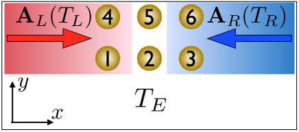
Figure 1: (Color online) Sketch of the set-up under consideration. The tight binding sites are labeled by 1 to 6 and are connected on the left and right side to two blackbody radiations at different temperature, $T_{L}$ and $T_{R}$. This system is embedded in an environment at temperature $T_{E}$.

As these blackbodies are far away from the system, their fields are a superposition of plane waves traveling in positive (or negative) $x$-direction, weighted according to their temperature, $\mathbb{A}_{L,R}(r,t)={\bf E_{0}}\int\mathrm{d}\Omega\sqrt{\Omega n(\Omega,T_{L,R})}\sin\left(\Omega t\pm kx+\phi(\Omega)\right),$ where ${\bf E_{0}}=E_{0}{\bf e}_{y}$, and $E_{0}$ is the strength of the corresponding electric field, ${\bf e}_{y}$ is the unit vector in the $y$ direction, and $\phi(\Omega)\in[0,2\pi]$ are uncorrelated random phase factors. Here, one might use more realistic, and also complicated, models for the correlation of thermal radiation Donges (1999); Bertilone (1996). This thermal radiation enters through the Peierls transformation of the hopping parameter $T^{A}_{ij}=T_{ij}\>\exp\left(-i\int_{\mathbb{R}_{i}}^{\mathbb{R}_{j}}\mathrm{d}\mathbb{r}\cdot(\mathbb{A}_{L}(r,t)+\mathbb{A}_{R}(r,t))\right)$, into the tight-binding hamiltonian,

$$\hat{H}_{S}=\sum_{\langle i,j\rangle}T^{A}_{ij}\hat{c}_{i}^{\dagger}\hat{c}_{j}.$$ (4)

Here, the operator $\hat{c}^{\dagger}_{i}$ creates an electron at site $i$ with position $\mathbb{R}_{i}$, and we assume a single electron to be present in the whole system. The sum $\langle i,j\rangle$ denotes summation over nearest neighbors only. The vector potentials $\mathbb{A}_{L}$ and $\mathbb{A}_{R}$ couple to the most leftwards and rightwards sites, respectively, and will introduce a local temperature gradient in the system. Note that in general the potentials penetrate into the system, however for this model system, we assume the external radiation is rapidly screened. For example, the core electrons in the tight-binding sites can be responsible for this screening.

The coupling to the environmental degrees of freedom is described by a master equation. For the coupling of an electronic system to the electro-magnetic field of the environment, the coupling operator $\hat{V}$ and bath-correlation function $C(\tau,t)$ can be derived from first principles by assuming the system to be embedded in a cavity at temperature $T_{E}$ Biele et al. (2014). The power spectrum, essentially the Fourier transform of the bath-correlation function, is given by $C_{\mathrm{env}}(\omega)={4|\omega|^{3}}/{c^{3}}\left[n(|\omega|,T_{E})+\theta(-\omega)\right]$ for $|\omega|<\omega_{c}$ where $\theta(\omega)$ is the Heaviside step function and $\omega_{c}$ is a cutoff frequency determined by the dimensions of the system. For $|\omega|>\omega_{c}$, the power spectrum is set to vanish. This cutoff is necessitated by the assumption made in the dipole approximation that the electromagnetic field is uniform in the region of space occupied by the system. The corresponding coupling operator, entering the master equation, is given by $\hat{V}=-\sum_{i,j}\mathbb{u}\cdot\langle W_{i}|\mathbb{r}|W_{j}\rangle\,\hat{c}_{i}^{\dagger}\hat{c}_{j},$ where $|W_{i}\rangle$ is the single-particle state localized at site $i$. As we are interested in the steady-state energy current through the system, we simplify the memory kernel of the non-Markovian master equation (3) by setting $\int_{0}^{t}\mathrm{d}\tau\hat{f}(\tau)[...]\rightarrow\int_{-\infty}^{\infty}\mathrm{d}\tau\hat{f}(t)[...]$. This approximation does not change the long-time limit of the equation of motion and hence is suitable to study steady-state dynamics Biele and D’Agosta (2012). In order to calculate the energy transport one has to define, via the continuity equation, an energy current in the system. With the local energy-density operator, $\hat{h}_{i}=\frac{1}{2}\sum_{\langle j\rangle}\big{(}T^{A}_{ij}\hat{c}^{\dagger}_{i}\hat{c}_{j}+\mathrm{h.c.}\big{)}$, one can define the total current in the $x$-direction via $\hat{j}^{x}_{T}=-\dot{\hat{h}}_{1}-\dot{\hat{h}}_{4}+\dot{\hat{h}}_{3}+\dot{\hat{h}}_{6}$, where $\dot{\hat{O}}=i[\hat{H}_{S},\hat{O}]+\partial_{t}\hat{O}$. As a first test of the novel thermal transport theory we examine the relaxation dynamics of the tight-binding system driven by a left and right blackbody radiation kept at temperature $k_{B}T=10\,a.u.$, the same temperature as the environment. We choose $T_{ij}=0.5\,a.u.$ as an energy-scale for the system, and for the coupling to the environment we set $\gamma=\sqrt{2/(\pi c^{3})}=0.05$. For the energy scale of the black-body radiations, we have normalized both left and right radiation with the time-averaged Poynting vector, $\langle S\rangle$, set to $15/(\mu_{0}\cdot c)$. In Fig. 2 the dynamics of the occupation probabilities of the eigenstates of the Hamiltonian (4) in the one-electron sector is shown for the unperturbed system (zero black-body field). One can see that the system relaxes towards a steady state. The steady state is characterized by zero energy transport in the system, which can be seen in the inset of Fig. 2.

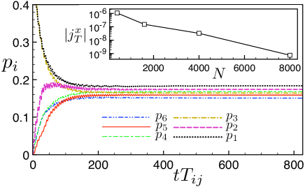
Figure 2: (Color online) Relaxation dynamics of the occupation probabilities of the eigenstates of the unperturbed Hamiltonian (4). This results have been obtained by averaging over $4\,000$ realizations of the stochastic noise. The inset shows the vanishing energy current through the system when the number of runs of the stochastic process, $N$, increases.

To further verify the theory we show one finds the expected turnover behavior as seen in Fig. 3 Hänggi and Borkovec (1990); Velizhanin et al. (2008). The turnover can be understood by considering that for small energy flux, when increasing the flux, more states are excited and can contribute to transport. On the other hand, at large fluxes, some of the states are fully occupied and are not able to contribute to transport anymore. At intermediate energy fluxes, a peak of the energy current must be achieved. In general, this behavior cannot be described by perturbative theories for thermal transport such as the Redfield theory Velizhanin et al. (2008). We have set the temperature gradient to $\Delta T=(T_{L}-T_{R})/2$.

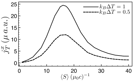
Figure 3: Dependence of the steady-state energy current on the coupling strength $\langle S\rangle$ for $k_{B}T_{E}=10$ and $N=4\,000$. A turnover in the energy current can be observed.

In Fig. 4 the energy current is plotted versus the introduced thermal gradient, $\Delta T$, from the black bodies. A linear dependence on the thermal gradient can be found for $\Delta T\ll T$ (see inset). At large $\Delta T$, a maximum in the energy current is reached. This implies that the system can sustain up to a maximum energy flow fixed the external conditions. Also, the position of the maximum of the energy current shifts to the right by increasing the temperature of the environment. This might be relevant for technological applications since the maximum efficiency can tuned according to the working conditions.

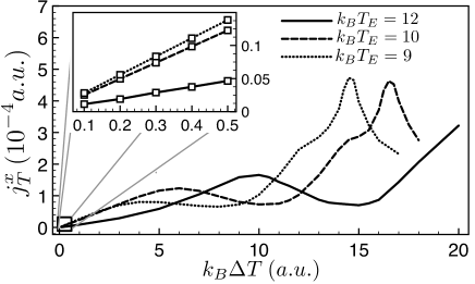
Figure 4: Energy current in the tight-binding system of Fig. 1 vs. temperature gradient introduced by the black-body radiations around the environmental temperature $T_{E}$. For this plot, we have used $\langle S\rangle=15/\mu_{0}c$ close to the maximum current of Fig. 3, and $N=4\,000$.

In conclusion, we have presented a novel theoretical framework to investigate thermal and energy transport, where the thermal imbalance in the system is introduced by two classical black body radiations. Our theory also includes a dissipative environment, where the system can gain energy from or dissipate to, in order to mimic the quantum nature of the photons. Due to the latter, we include the fundamental concept of thermal relaxation of the system, which is not included in other thermal transport theories. The theory can also be used in different set-ups, e.g., we can consider one blackbody only, to adapt to different experiments. Finally, as our formalism relies on the knowledge of the external vector potential, we can foresee that its combination with the powerful techniques of TDCDFT will provide a novel ab-initio tool to study thermal transport in many-body systems, and possibly pave the way to define a local temperature. In addition, by utilizing a recent development in combining Time-Dependent Density Functional theory and quantum electro-dynamics Ruggenthaler et al. (2014), we can go beyond the mean-field description of the environment. Moreover, within the same formalism we can investigate phonon thermal transport, thereby combined with the TDCDFT, our model provides a unified way to investigate ab-initio electrical and thermal transport beyond linear response. Non-linear regimes are important since in seeking for, e.g., the maximum efficiency of a thermoelectric energy converter, we might need to go beyond the standard linear response D’Agosta (2013). Since our formalism is fully dynamic we have direct access to transient regimes, to how the steady state is approached, and to whether or not this steady state is unique or depends on the history of the system Stefanucci (2007).