LARGE DEVIATIONS FOR GENERALIZED POLYA URNS WITH ARBITRARY URN FUNCTION

Abstract.

We consider a generalized two-color Polya urn (black and withe balls) first introduced by Hill, Lane, Sudderth [HLS1980], where the urn composition evolves as follows: let $\pi:\left[0,1\right]\rightarrow\left[0,1\right]$, and denote by $x_{n}$ the fraction of black balls after step $n$, then at step $n+1$ a black ball is added with probability $\pi\left(x_{n}\right)$ and a white ball is added with probability $1-\pi\left(x_{n}\right)$. Originally introduced to mimic attachment under imperfect information, this model has found applications in many fields, ranging from Market Share modeling to polymer physics and biology.

In this work we discuss large deviations for a wide class of continuous urn functions $\pi$. In particular, we prove that this process satisfies a Sample-Path Large Deviations principle, also providing a variational representation for the rate function. Then, we derive a variational representation for the limit

$$\phi\left(s\right)=\lim_{n\rightarrow\infty}{\textstyle\frac{1}{n}}\log\mathbb{P}\left(nx_{n}=\left\lfloor sn\right\rfloor\right),\,s\in\left[0,1\right],$$

where $nx_{n}$ is the number of black balls at time $n$, and use it to give some insight on the shape of $\phi\left(s\right)$. Under suitable assumptions on $\pi$ we are able to identify the optimal trajectory. We also find a non-linear Cauchy problem for the Cumulant Generating Function and provide an explicit analysis for some selected examples. In particular we discuss the linear case, which embeds the Bagchi-Pal Model [BP1983], giving the exact implicit expression for $\phi$ in terms of the Cumulant Generating Function.

1. Introduction.

Urns are simple probabilistic models that had a broad theoretical development and applications for several decades, gaining a prominent position within the framework of adaptive stochastic processes. In general, single-urn schemes are Markov chains that start with a set (urn) containing two or more elements of different types: at each step a number of elements is added or removed with some probabilities depending on the composition of the urn. Since their introduction these models where intended to describe phenomena where an underlying tree growth is present [Pem2007, Mam2003, JK1977, Mam2008].

Given the general definition above, an impressive number of variants have been introduced, depending on the number of colors, extraction and replacement rules, etc. This work focuses on Large Deviations Principles (LDP) for a generalization of the classical Polya-Eggenberger two-colors urn scheme, first introduced by Hill, Lane and Sudderth [HLS1980, HLS1987]. Let us consider an infinite capacity urn which contains two kinds of elements, say black and white balls, and denote by $X_{n}:=\left\{X_{n,k}:1\leq k\leq n\right\}$ the number of black balls during the urn evolution from time $0$ to $n$: at time $k$ there are $k$ balls in the urn, $X_{n,k}$ of which are black. Given a map $\pi:\left[0,1\right]\rightarrow\left[0,1\right]$ (usually referred to as urn function) the urn evolves as follows: let $x_{n,k}:=k^{-1}X_{n,k}$, $1\leq k\leq n$ be the fraction of black balls in the urn at step $k$, then a new ball is added at step $k+1$, whose color is black with probability $\pi\left(x_{n,k}\right)$ and white with probability $1-\pi\left(x_{n,k}\right)=\bar{\pi}\left(x_{n,k}\right)$ (hereafter we denote the complementary probability by an upper bar),

(1.1) $$X_{n,k+1}=\left\{\begin{array}[]{l}X_{n,k}+1\\ X_{n,k}\end{array}\begin{array}[]{l}with\ probability\\ with\ probability\end{array}\begin{array}[]{l}\pi\left(x_{n,k}\right),\\ \bar{\pi}\left(x_{n,k}\right).\end{array}\right.$$

Apart form the wide range of behaviors depending on the choice of the urn function, which makes this generalized urn scheme challenging and rich by itself, attention arises from its relevance to branching phenomena, stochastic approximation and reinforced random walks [HLS1980, HLS1987, Gou1993, KB1997, Mam2003, Pem2007], as well as in in Market Share modeling [DEK1994, AEK1983, AEK1987b, AEK1986, AEK1986b, AEK1987] and other fields [KK2001, CL2009, Oliv2008, DFM2002]. We remark it has also been generalized to multicolor urns, whose strong convergence properties have been investigated by Arthur et Al. in a series of papers [AEK1986, AEK1986b, AEK1987], but in the present work we restrict our attention to the two-colors case.

The paper is organized as follows: in this introductory section we briefly review the main known results about the Generalized Polya (GP) urn of Hill, Lane and Sudderth, discussing the classes of urn functions we will consider and introducing some notation. Our results on large deviations are in Section 2: in particular, we will present our theorems concerning the Sample Path Large Deviations Principles, a large deviations analysis for the event $\left\{X_{n,n}=\left\lfloor sn\right\rfloor\right\}$, $s\in\left[0,1\right]$ and the Cumulant Generating Function (CGF), also discussing some applications to paradigmatic examples from literature. All proofs have been collected in a dedicated section (Section 3) which contains almost all the technical features of this work.

1.1. The urn function $\pi$.

In the following we formally present the GP urns of Hill, Lane and Shuddery, and introduce some non-standard notation which will be useful when dealing with LDPs: we tried to reduce new notation to minimum, keeping the common urn terminology everywhere this was possible.

As we shall see, the initial conditions do not affect the LDPs for the class of urn functions we will consider, unless the urn has some intervals of $s$ for which $\pi\left(s\right)=1$ or $0$. Then, if not specified otherwise, in this work we set $X_{n,1}$ to be a random variable uniformly distributed on $\left[0,1\right]$ by convention, ie

(1.2) $$\mathbb{P}\left(X_{n,1}\in\left[s_{1},s_{2}\right]\right):=\left|s_{2}-s_{1}\right|,\,\forall\left[s_{1},s_{2}\right]\subset\left[0,1\right].$$

We remark that in the above definition $X_{n,1}$ does not represent the number of black balls at the initial stage of the urn evolution, it is just a convenient initial condition for the Eq. (1.3) below. We will further elaborate the effect of realistic initial conditions on the LDPs in Section 2, after the statement of Corollary 2. That said, our process $X_{n}:=\left\{X_{n,k}:1\leq k\leq n\right\}$ is the Markov Chain with transition matrix:

(1.3) $$\mathbb{P}\left(X_{n,k+1}=X_{n,k}+i|\,X_{n,k}=j\right):=\pi\left(j/k\right)\mathbb{I}_{\left\{i=1\right\}}+\bar{\pi}\left(j/k\right)\mathbb{I}_{\left\{i=0\right\}}.$$

We denote by $\delta X_{n}$ the associated sequence $\delta X_{n,k}:=X_{n,k+1}-X_{n,k}\in\left\{0,1\right\}$ for $0\leq k\leq n-1$. For notational convenience, the dependence on $\pi$ is not specified. Throughout this work we will consider a sub-class $\mathcal{U}$ of continuous functions $\pi$: $\left[0,1\right]\rightarrow\left[0,1\right]$ defined as follows:

Definition.

We say that $\pi$: $\left[0,1\right]\rightarrow\left[0,1\right]$ continuous belongs to $\mathcal{U}$ if some function $f>0$ with

(1.4) $$\lim_{\epsilon\rightarrow 0}\epsilon\int_{\epsilon}^{1}{\textstyle dz}\,f\left(z\right)/z^{2}=0$$

exists such that $\left|\pi\left(x+\delta\right)-\pi\left(x\right)\right|\leq f\left(\left|\delta\right|\right)$ for $\delta\rightarrow 0$, $x\in\left[0,1\right]$. For example, in the Polya-Eggenberger urn we can take $f\left(z\right)=z$ and the above condition becomes $\lim_{\epsilon\rightarrow 0}\epsilon\log\left(\epsilon\right)=0$.

Even if this class of functions is slightly smaller than those considered in [HLS1980, Pem2007, Mam2003, Pem1991], where most results are obtained for continuous functions, it still includes all Lipschitz and $\alpha-$Hölder functions. This class has been constructed to include most of the interesting cases that can be described by urn functions while keeping properties that allow a reasonably straight application of the Varadhan lemma. We will discuss this in Section 3.

In the following we introduce some new notation which is intended to ease the description of our results, as well as the limit properties of $X_{n}$. Define the following sets:

(1.5) $$C_{\pi}:=\left\{s\in\left(0,1\right):\,\pi\left(s\right)=s\right\},\,\partial C_{\pi}:=C_{\pi}\setminus\mathrm{int}\left(C_{\pi}\right),$$

where $\mathrm{int\left(C_{\pi}\right)}$ is the interior of $C_{\pi}$. We will refer to the elements of $C_{\pi}$ as contacts. Note that for the considered urn functions $C_{\pi}$ may not be a set of isolated points, since our definition of $\mathcal{U}$ allows $\pi\left(s\right)=s$ for some interval $s\in\left[s_{1},s_{2}\right]$ (see the region $K_{\pi,3}$ in Figure 1.1). On the contrary $\partial C_{\pi}$ is always a finite set of isolated points since it collects the boundaries of the regions in which $\pi\left(s\right)-s$ has a definite sign. We denote by $N:=\left|\partial C_{\pi}\right|$ the number of such points in $\partial C_{\pi}$ for a given $\pi$.

We can further distinguish the elements of $\partial C_{\pi}$ by considering the behavior of $\pi\left(s\right)$ in their neighborhood: to do so, we will introduce a partition of the interval $\left[0,1\right]$. We remark that the notation we are going to define is not a standard of urn literature, but it will prove useful in describing of our results when dealing with optimal trajectories. First, let us organize the elements of $\partial C_{\pi}$ by increasing order, labeling them as

(1.6) $$\partial C_{\pi}=:\left\{s_{i},1\leq i\leq N:\,s_{i}<s_{i+1}\right\}.$$

Then, we can define the following sequence of intervals (see Figure 1.1)

(1.7) $$K_{\pi}:=\left\{K_{\pi,i},\,0\leq i\leq N:\,K_{\pi,0}:=\left(0,s_{1}\right),K_{\pi,N}:=\left(s_{N},1\right),\,K_{\pi,j}:=\left(s_{j},s_{j+1}\right)\right\}.$$

By definition of $\partial C_{\pi}$, the above intervals are such that $\pi\left(s\right)-s$ does not change sign for $s\in K_{\pi,i}$. Then we can associate a variable $a_{\pi,i}\in\left\{-1,0,1\right\}$ to each interval $K_{\pi,i}$ which expresses the sign of $\pi\left(s\right)-s$. We denote such sequence by

(1.8) $$A_{\pi}:=\{a_{\pi,i},\,0\leq i\leq N:\,a_{\pi,i}={\textstyle\frac{\pi\left(s\right)-s}{\left|\pi\left(s\right)-s\right|}\mathbb{I}_{\left\{\pi\left(s\right)\neq s\right\}}},\,s\in K_{\pi,i}\}.$$

Some words should be spent on the correct use of this notation when the urn function has $\pi\left(0\right)=0$ or $\pi\left(1\right)=1$, or both. Consider the first case: if $\pi\left(0\right)=0$ then the smallest element of $\partial C_{\pi}$ is $s_{1}=0$. Following our definition of $K_{\pi,0}$ as open interval we would have that $K_{\pi,0}=\textrm{\O}$ and $a_{\pi,0}$ not well defined. To patch this, we set by convention that $a_{\pi,0}=1$ if $K_{\pi,0}=\textrm{\O}$ and $a_{\pi,N}=-1$ if $K_{\pi,N}=\textrm{\O}$.

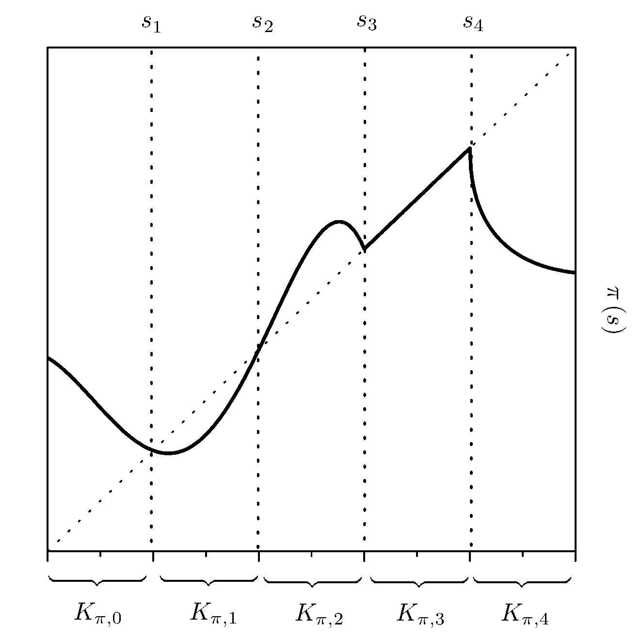
Figure 1.1. Example of urn function $\pi\in\mathcal{U}$ to illustrate the notation introduced in Eq.s (1.7), (1.6). For the function above we have $C_{\pi}=\left\{1/5,\,2/5,\,3/5,\,4/5\right\}\cup\left(3/5,\,4/5\right)$, then $\partial C_{\pi}=\left\{1/5,\,2/5,\,3/5,\,4/5\right\}$, $K_{\pi,0}=\left[0,1/5\right)$, $K_{\pi,4}=\left(4/5,\,1\right]$, $K_{\pi,i}:=\left(i/5,\,\left(i+1\right)/5\right)$, $i\in\left\{1,2,3\right\}$ and $A_{\pi}=\left\{1,\,-1,\,1,\,0,\,-1\right\}$. Also, $s_{1}=1/5\in C_{\pi}\left(+,-\right)$ is a downcrossing, $s_{2}=2/5\in C_{\pi}\left(-,+\right)$ is an upcrossing, $s\in\left(3/5,4/5\right)$ is a dense region of Polya-like contacts $C_{\pi}\left(0,0\right)$ while $s_{3}=3/5$, $s_{4}=4/5$ are its left and right boundaries $C_{\pi}\left(+,0\right)$, $C_{\pi}\left(0,-\right)$ respectively.

Using the above notation we can now define the subsets $C_{\pi}\left(\alpha,\beta\right)$ of those $s\in\partial C_{\pi}$ such that $\alpha\in\left\{+,0,-\right\}$ is the sign of $\pi{\textstyle\left(s^{\prime}\right)-s^{\prime}}$ for $s^{\prime}-s\rightarrow 0^{-}$ and $\beta\in\left\{+,0,-\right\}$ is the sign of $\pi{\textstyle\left(s^{\prime}\right)-s^{\prime}}$ for $s^{\prime}-s\rightarrow 0^{+}$.

(1.9) $$C_{\pi}\left(\alpha,\beta\right):=\left\{s_{i}\in\partial C_{\pi}:\,\mathrm{sign}\left(a_{\pi,i-1}\right)=\alpha,\,\mathrm{sign}\left(a_{\pi,i}\right)=\beta\right\}$$

References [HLS1980, Pem2007, Mam2003, Pem1991] call $C_{\pi}\left(+,-\right)$ and $C_{\pi}\left(-,+\right)$ respectively downcrossings and upcrossings, while $C_{\pi}\left(+,+\right)$ and $C_{\pi}\left(-,-\right)$ are touchpoints. Note that our classification also allows contacts of the kind $C_{\pi}\left(\alpha,0\right)$ and $C_{\pi}\left(0,\beta\right)$, which are the boundaries of those intervals $K_{\pi,i}$ for which $\pi\left(s\right)=s$ ($a_{\pi,i}=0$).

1.2. Strong convergence.

Here we review some of the main known results on strong convergence, ie, on the almost sure convergence of $x_{n,n}$. This topic has been widely investigated in [HLS1980, HLS1987, Gou1993, Pem1991, Mam2003, Pem2007]). As example, consider the simplest non trivial urn model, the so called Polya-Eggenberger urn [EP1923], which evolves as follows: at each step draw a ball, if it is black then add a black ball, and add a white one otherwise. This urn is represented in our context by the urn function $\pi\left(s\right)=s$. In this case $\mathbb{E}\left(x_{n,k+1}|x_{n,k}\right)=x_{n,k}$, so that $x_{n,k}$ is a martingale and $\lim_{n}x_{n,n}$ exists almost surely.

The existence of $\lim_{n}x_{n,n}$ has been shown in [HLS1980] for a wider class of urn functions (including some non-continuous $\pi$). In [HLS1980] it has been shown that if $\pi$ is a continuous function then $\lim_{n}x_{n,n}$ exists almost surely, and $\lim_{n}x_{n,n}\in C_{\pi}$. The same result holds if $\pi$ is non-continuous, provided the points $s$ where $\pi\left(s\right)-s$ oscillates in sign are not dense in an interval.

Clearly, not all the points of $C_{\pi}$ can be the limit of $x_{n,n}$ and several efforts were made to determine whether a point belongs to the support of $\lim_{n}x_{n,n}$ for a given $\pi$ [HLS1980, Pem1991]. We say that $s\in\left[0,1\right]$ belongs to the support of $\lim_{n}x_{n,n}$ if $\mathbb{P}\left(\left|\lim_{n}x_{n,n}-s\right|<\delta\right)>0$, $\forall\delta>0$. In general, we can summarize from [HLS1980, Pem1991] what is known about the support of $\lim_{n}x_{n,n}$ in our setting ($\pi\in\mathcal{U}$ and $X_{n,1}$ uniform on $\left[0,1\right]$). Let $X_{n}$ be the urn process generated by the urn function $\pi\in\mathcal{U}$, and define $\Delta_{\pi,\epsilon}\left(s\right):=\epsilon^{-1}\left[\pi\left(s+\epsilon\right)-\pi\left(s\right)\right]$. Then the limit $\lim_{n}x_{n,n}$ exists almost surely and

1. Downcrossings $C_{\pi}\left(+,-\right)$ always belong to the support of $\lim_{n}x_{n,n}$ while upcrossings $C_{\pi}\left(-,+\right)$ never do.

2. If $s\in C_{\pi}\left(+,+\right)$, then it belongs to the support of $\lim_{n}x_{n,n}$ if and only if some $\delta>0$ exists such that $\Delta_{\pi,\epsilon}\left(s\right)\in\left(1/2,1\right)$ for $\epsilon\in\left(-\delta,0\right)$.

3. If $s\in C_{\pi}\left(-,-\right)$, then it belongs to the support of $\lim_{n}x_{n,n}$ if and only if some $\delta>0$ exists such that $\Delta_{\pi,\epsilon}\left(s\right)\in\left(1/2,1\right)$ for $\epsilon\in\left(0,\delta\right)$.

The proof that downcrossings belong to the support of $\lim_{n}x_{n,n}$ while upcrossings don’t can be found in reference [HLS1980]: it involves Markov chain coupling together with martingale analysis. The statement that touchpoints $C_{\pi}\left(+,+\right)$ with $1/2<\Delta_{\pi,\epsilon}\left(s\right)<1$ from the left ($\epsilon<0$) and $C_{\pi}\left(-,-\right)$ with $1/2<\Delta_{\pi,\epsilon}\left(s\right)<1$ from the right ($\epsilon>0$) belong to the support of $\lim_{n}x_{n,n}$ has been proved in [Pem1991] by Pemantle. This seemingly paradoxical statement is actually a deep observation about the dynamics of the process: if the condition on $\Delta_{\pi,\epsilon}\left(s\right)$ is fulfilled, then $x_{n,n}$ converges so slowly to $s\in C_{\pi}\left(+,+\right)$ from the left (to $s\in C_{\pi}\left(-,-\right)$ from the right) that it almost surely never crosses this point, accumulating in its left (right) neighborhood. If not, then $x_{n,n}$ crosses $s$ in finite time almost surely, and gets pushed away from the other side toward the closest stable equilibrium (ie, the closest point that belongs to the support of $\lim_{n}x_{n,n}$ ).

Even if we left out the cases $C_{\pi}\left(\alpha,0\right)$, $C_{\pi}\left(0,\beta\right)$ and $s\in K_{\pi,i}$ with $a_{\pi,i}=0$ from the above statement it is clear that they always belong to the support of $\lim_{n}x_{n,n}$ since in some neighborhood of these points the process behaves like a Polya-Eggenberger urn.

We remark that almost sure convergence is strongly affected by initial conditions: since a detailed discussion of this topic would be far from the scope of this work, we defer to the reviews [HLS1980, Pem2007, Mam2003, Pem1991].

2. Main results.

While the almost sure convergence properties of such urns are quite well understood also in multicolor generalizations (see [AEK1986, AEK1986b, AEK1987]), Large Deviations properties are not. Apart from the Polya-Eggenberger urn, for which we can explicitly compute the exact urn composition at each time, to the best of our knowledge large deviations results in urn models have been pioneered by Flajolet et Al. [FGP2005, FDP2006, HKP2007], which provided a detailed analysis of the Bagchi-Pal urn using generating function methods. Since then other authors extended this approach to many related models (of particular interest is [MM2012], a Bagchi-Pal urn with stochastic reinforcement matrix). Another early work on Large Deviations has been provided by Bryc et Al. in [BMS2009], where a special Bagchi-Pal type urn is studied as model for preferential attachment and an explicit expression of the Cumulant Generating Function is obtained in integral form (see the end of this section for an introduction to the Bagchi-Pal model).

This section mostly contains the statements of our results. Most of the proofs of the following statements are grouped in Section 3: we will specify where to find them.

2.1. Sample-Path Large Deviation Principle.

As preliminary result, we need a Sample-Path Large Deviation principle which holds for any $\pi\in\mathcal{U}$. Then, define the function $\chi_{n}:\left[0,1\right]\rightarrow\left[0,1\right]$ as follows:

(2.1) $$\chi_{n}:=\left\{\chi_{n,\tau}=n^{-1}\left[X_{n,\left\lfloor n\tau\right\rfloor}+\left(n\tau-\left\lfloor n\tau\right\rfloor\right)\delta X_{n,\left\lfloor n\tau\right\rfloor}\right]:\tau\in\left[0,1\right]\right\},$$

where $\left\lfloor\cdot\right\rfloor$ denotes the lower integer part, and introduce the subspace of Lipschitz-continuous functions

(2.2) $$\mathcal{Q}:=\left\{\varphi\in C\left(\left[0,1\right]\right):\,\varphi_{0}=0,\,\varphi_{\tau+\delta}-\varphi_{\tau}\in\left[0,\delta\right],\,\delta>0,\,\tau\in\left[0,1\right]\right\},$$

where $C\left(\left[0,1\right]\right)$ is the set of continuous functions on $\left[0,1\right]$. Denote by $\left\|\varphi\right\|:=\sup_{\tau\in\left[0,1\right]}\left|\varphi_{\tau}\right|$ the usual supremum norm, and consider the normed metric space $\left(\mathcal{Q},\,\left\|\cdot\right\|\right)$. We show that a good rate function $I_{\pi}:\mathcal{Q}\rightarrow\left[0,\infty\right)$ exists such that for every Borel subset $\mathcal{B}\subseteq\mathcal{Q}$:

(2.3) $$\liminf_{n\rightarrow\infty}\,n^{-1}\log\mathbb{P}\left(\chi_{n}\in\mathrm{int}\left(\mathcal{B}\right)\right)\geq-\inf_{\varphi\in\mathrm{int}\left(\mathcal{B}\right)}I_{\pi}\left[\varphi\right],$$

(2.4) $$\limsup_{n\rightarrow\infty}\,n^{-1}\log\mathbb{P}\left(\chi_{n}\in\ \mathrm{cl}\left(\mathcal{B}\right)\right)\leq-\ \,\inf_{\varphi\in\mathrm{cl}\left(\mathcal{B}\right)}I_{\pi}\left[\varphi\right].$$

To describe the rate function we introduce a functional $S_{\pi}:\mathcal{Q}\rightarrow\left(-\infty,0\right]$, defined as follows:

(2.5) $$S_{\pi}\left[\varphi\right]:=\int_{\tau\in\left[0,1\right]}\left[\,d\varphi_{\tau}\,\log\pi\left(\varphi_{\tau}/\tau\right)+d\tilde{\varphi}_{\tau}\,\log\bar{\pi}\left(\varphi_{\tau}/\tau\right)\right],$$

where we denoted $\bar{\pi}\left(s\right)=1-\pi\left(s\right)$ and $\tilde{\varphi}_{\tau}=\tau-\varphi_{\tau}$. Then, the following theorem gives the Sample-Path LDP for $\chi_{n}$:

Theorem 1.

Let $\pi\in\mathcal{U}$, $\varphi\in\mathcal{Q}$, define the function $H\left(s\right):=s\log s+\bar{s}\log\bar{s}$, and the functional $J:\mathcal{Q}\rightarrow\left[-\log 2,\infty\right)$ as follows:

(2.6) $$J\left[\varphi\right]=\left\{\begin{array}[]{l}\int_{0}^{1}d\tau\,H\left(\dot{\varphi}_{\tau}\right)\\ \infty\end{array}\ \begin{array}[]{l}if\ \varphi\in\mathcal{AC}\\ otherwise,\end{array}\right.$$

where $\mathcal{AC}$ is the class of absolutely continuous functions (we assume the same definition given in Theorem 5.1.2 of [DZ1998]) and $\dot{\varphi}_{\tau}:=\frac{d\varphi_{\tau}}{d\tau}$. Also, define the good rate function

(2.7) $$I_{\pi}\left[\varphi\right]=J\left[\varphi\right]-S_{\pi}\left[\varphi\right],$$

with $S_{\pi}$ as in Eq. (2.5). Then, the law of $\chi_{n}$ with initial condition $X_{n,1}$ of Eq. (1.2) uniformly distributed on the interval $\left[0,1\right]$ satisfies a Sample-Path LDP as in Eq.s (2.3) and (2.4), with good rate function $I_{\pi}\left[\varphi\right]$.

The proof is quite standard, and based on a change of measure and an application of the Varadhan Integral Lemma plus some surgery on the set $\mathcal{Q}$ to a priori exclude those trajectories which create issues in proving the continuity of $S_{\pi}\left[\varphi\right]$ on $\left(\mathcal{Q},\left\|\cdot\right\|\right)$ (see the approximation argument of Lemma 14).

Let us now consider a process with some specific initial condition, say $X_{n,m}=X_{m}^{*}$ for some $0<m\leq n$ and $0\leq X_{m}^{*}\leq m$. If we call by $\chi_{n}^{*}$ a process defined as in Eq. (2.1) with the additional condition $\mathbb{P}\left(\chi_{n,m/n}=n^{-1}X_{m}^{*}\right)=1$, then we can resume the effects of such constraint in the following corollary

Corollary 2.

Let $\pi\in\mathcal{U}$ and denote by $\chi_{n}^{*}$ a process defined as in Eq. (2.1) with the additional condition that $\chi_{n,m/n}^{*}=n^{-1}X_{m}^{*}$ for some $0<m\leq n$ and $0\leq X_{m}^{*}\leq m$. Define $0\leq z_{-}^{*}<z_{+}^{*}\leq 1$ as follows

(2.8) $$z_{-}^{*}:=\liminf_{n\rightarrow\infty}\left\{z_{-}:\,\mathbb{P}\left(X_{n,n}\leq z_{-}n\,|\,X_{n,m}=X_{m}^{*}\right)>0\right\},$$

(2.9) $$z_{+}^{*}:=\limsup_{n\rightarrow\infty}\left\{z_{+}:\,\mathbb{P}\left(X_{n,n}\geq z_{+}n\,|\,X_{n,m}=X_{m}^{*}\right)>0\right\},$$

and a modified urn function $\pi^{*}$

(2.10) $$\pi^{*}\left(s\right):=\mathbb{I}_{\{s\in\left[0,z_{-}^{*}\right)\}}+\pi\left(s\right)\mathbb{I}_{\{s\in\left[z_{-}^{*},z_{+}^{*}\right]\}}.$$

Then, the law of $\chi_{n}^{*}$ with initial condition $x_{n,m}=m^{-1}X_{m}^{*}$ satisfies a Sample-Path LDP with good rate function $I_{\pi^{*}}$, as for $\chi_{n}$ with $X_{n,1}$ uniform on $\left[0,1\right]$ and $\pi^{*}$ in place of $\pi$.

The above results tell us that initial conditions of the kind $\mathbb{P}\left(X_{n,m}=k\right)=\mathbb{I}_{\left\{k=X_{m}^{*}\right\}}$ can affect the rate function if and only if $\pi\left(s\right)$ is $0$ or $1$ for some values of $s$. We can easily convince ourselves of this by observing that if $\pi\in\left(0,1\right)$ then $X_{n,n}$ can reach any point in $\left\{X_{m},X_{m}+1,\,...\,,X_{m}+\left(n-m\right)\right\}$ in finite time $n-m$ from $X_{n,m}$, while the presence of intervals with $\pi\left(s\right)=0$ or $1$ can prevent the process from crossing some values. The proof of the above corollary is in Section 3.1.1. Notice that we can define $z_{-}^{*}$ and $z_{+}^{*}$ also for $X_{n,1}$ uniform on $\left[0,1\right]$, and in this case we can take

(2.11) $$z_{-}^{*}:={\textstyle\inf}\left\{s:\pi\left(s\right)<1\right\},\,z_{+}^{*}:=\sup\left\{s:\pi\left(s\right)>0\right\}.$$

In the following we will consider the above definition, unless some different initial condition is specified.

Before going ahead some words should be spent on non homogeneous urn functions. Then, take $\pi\in\mathcal{U}$ with $\pi\in\left(0,1\right)$ and consider a sequence of urn functions $\left\{\pi_{n}\in\mathcal{U}:\,n\geq 0\right\}$ such that for every $n\geq 0$ we have $\pi_{n}\left(s\right)\in\left(0,1\right)$ for $s\in\left[0,1\right]$ and $\pi_{n}\rightarrow\pi$ uniformly on $\left[0,1\right]$. In Section 3.1.1 we show that

Corollary 3.

Take $\pi\in\mathcal{U}$ with $\pi\left(s\right)\in\left(0,1\right)$ and let $\pi_{n}\in\mathcal{U}$ such that $\pi_{n}\left(s\right)\in\left(0,1\right)$ and $\left|\pi_{n}\left(s\right)-\pi\left(s\right)\right|\leq\delta_{n}$, $\lim_{n}\delta_{n}=0$ for all $s\in\left[0,1\right]$. Then, the non homogeneous urn process defined by $\pi_{n}$ satisfies the same Sample-Path LDP of $\pi$.

We restricted our statement to urns with $\pi\left(s\right)\in\left(0,1\right)$, $\pi_{n}\left(s\right)\in\left(0,1\right)$ to avoid some technical issues which would arise if we consider the whole set $\mathcal{U}$, but it is possible to generalize this result on the basis of the same considerations made for Theorem 1. We hope to address this extension in a future work.

2.2. Entropy of the event $X_{n,n}=\left\lfloor sn\right\rfloor$.

Our main interest in Theorem 1 comes from the fact that Sample-Path LDPs allow to approach some important Large Deviation questions about the urn evolution from the point of view of functional analysis. In this work our attention will mainly focus on the entropy of the event $X_{n,n}=\left\lfloor sn\right\rfloor$, $s\in\left[0,1\right]$. First we show that the limit

(2.12) $$\phi\left(s\right):=\lim_{n\rightarrow\infty}n^{-1}\log\mathbb{P}\left(X_{n,n}=\left\lfloor sn\right\rfloor\right),$$

exists for every $\pi\in\mathcal{U}$, and has the following variational representation:

Theorem 4.

The limit $\phi\left(s\right)$ defined in Eq. (2.12) exists for any $\pi\in\mathcal{U}$ and is given by the variational problem

(2.13) $$\phi\left(s\right)=-\inf_{\varphi\in\mathcal{Q}_{s}}I_{\pi}\left[\varphi\right],$$

where $\mathcal{Q}_{s}:=\left\{\varphi\in\mathcal{Q}:\,\varphi_{1}=s\right\}$ and $I_{\pi}$ is the rate function of Theorem 1. If we consider an initial condition $\chi_{n,m/n}^{*}=n^{-1}X_{m}^{*}$ for some $0<m\leq n$ and $0\leq X_{m}^{*}\leq m$ the same result holds with $I_{\pi^{*}}$ in place of $I_{\pi}$ and $\pi^{*}$ as in Corollary 2.

Notice that Theorem 1 can not be directly applied to the Eq. (2.12) in order to obtain Theorem 4, since this is a stronger statement than what one obtains by the contraction principle. To prove Theorem 4 we integrated Theorem 1 with a combinatorial argument: the proof can be found in Section 3.2.1.

2.2.1. Optimal trajectories.

Since the variational problem in Theorem 4 heavily depends on the choice of $\pi$, a general characterization of $\phi\left(s\right)$ would be a quite hard nut to crack. Anyway, we still can prove many interesting facts on the shape of $\phi\left(s\right)$. Most important, we can prove that $\phi\left(s\right)=0$ when $s\in\left[\,\inf C_{\pi},\,\sup C_{\pi}\right]$ and $\phi\left(s\right)<0$ otherwise.

Corollary 5.

For any $\pi\in\mathcal{U}$: $\phi\left(s\right)=0$ when $s\in\left[\,\inf\,C_{\pi},\,\sup\,C_{\pi}\right]$ and $\phi\left(s\right)<0$ otherwise, where $C_{\pi}$ is the contact set of $\pi$ defined by Eq. (1.5). Moreover, $\phi\left(s\right)>-\infty$ for $s\in\left(z_{-}^{*},\inf C_{\pi}\right)$ and $s\in\left(\sup\,C_{\pi},z_{+}^{*}\right)$, while $\phi\left(s\right)=-\infty$ for $s\in\left[0,z_{-}^{*}\right]$ and $s\in\left[z_{+}^{*},1\right]$.

The above corollary is obtained by proving that we can find a trajectory $\varphi^{*}\in\mathcal{Q}_{s}$ such that $I_{\pi}\left[\varphi^{*}\right]=0$ for any $s\in\left[\,\inf C_{\pi},\,\sup C_{\pi}\right]$, while this is not possible if $s\in K_{\pi,0}$ or $K_{\pi,N}$. Also, we are able to give an explicit characterization of the optimal trajectories $\varphi^{*}$. We enunciate this result in two separate corollaries: the first deals with trajectories that end in $s\in K_{\pi,i}$, $1\leq i\leq N-1$, while the second deals with trajectories that end in $s\in\partial C_{\pi}$ (as we shall see, Corollary 5 is an almost direct consequence of the following two) .

Corollary 6.

Let $K_{\pi}$, $A_{\pi}$ be as in Eq.s (1.7), (1.8). For any $s\in K_{\pi,i}$ a zero-cost trajectory $\varphi^{*}\in\mathcal{Q}_{s}$ with $\tau^{-1}\varphi_{\tau}^{*}\in K_{\pi,i}\cup\partial K_{\pi,i}$, $\tau\in\left[0,1\right]$ exists such that $I_{\pi}\left[\varphi^{*}\right]=0$, and it can be constructed as follows. If $a_{\pi,i}=0$ then we can take $\varphi^{*}=s\tau$ as in the Polya-Eggenberger urn. If $a_{\pi,i}\neq 0$ let

(2.14) $$F_{\pi}\left(s,u\right):=\int_{u}^{s}\frac{dz}{\pi\left(z\right)-z}.$$

Also, for $s\in K_{\pi,i}$ define the constants

(2.15) $$s_{i}^{*}:=\mathbb{I}_{\left\{a_{\pi,i}=1\right\}}\inf K_{\pi,i}+\mathbb{I}_{\left\{a_{\pi,i}=-1\right\}}\sup K_{\pi,i},$$

(2.16) $$\tau_{s,i}^{*}:=\exp\left(-{\textstyle\lim_{\,a_{\pi,i}(u-s_{i}^{*})\rightarrow 0^{+}}\left|F_{\pi}\left(s,u\right)\right|}\right).$$

and denote by $F_{\pi,s}^{-1}$ the inverse function of $F_{\pi}\left(s,u\right)$ for $u\in K_{\pi,i}\cup\partial K_{\pi,i}$:

(2.17) $$F_{\pi,s}^{-1}:=\left\{F_{\pi,s}^{-1}\left(q\right),\,q\in\left[0,\log\left(1/\tau_{s,i}^{*}\right)\right):\,F_{\pi}\left(s,F_{\pi,s}^{-1}\left(q\right)\right)=q\right\}.$$

Then, if $a_{\pi,i}\neq 0$ the zero-cost trajectory is given by $\varphi_{\tau}^{*}=\tau u_{\tau}^{*}$, with

(2.18) $$u_{\tau}^{*}:=F_{\pi,s}^{-1}\left(\log\left(1/\tau\right)\right)\,\mathbb{I}_{\left\{\tau\in\left(\tau_{s,i}^{*},1\right]\right\}}+s_{i}^{*}\,\mathbb{I}_{\left\{\tau\in\left[0,\tau_{s,i}^{*}\right]\right\}}.$$

The proof relies on the fact that any $\varphi^{*}$ for which $I_{\pi}\left[\varphi^{*}\right]=0$ must satisfy the Homogeneous equation $\dot{\varphi}_{\tau}^{*}=\pi\left(\varphi_{\tau}^{*}/\tau\right)$. This is shown in Section 3.2.2.

The above corollary states that the optimal strategy to achieve the event $\left\{X_{n,n}=\left\lfloor sn\right\rfloor\right\}$, $s\in\left[\,\inf\,C_{\pi},\,\sup\,C_{\pi}\right]$ emanates from the closest unstable equilibrium point which is on the left of $s$ if $\pi\left(s\right)$$<s$ and on the right if $\pi\left(s\right)>s$, see Figure 2.1 for an example. Notice that $u_{\tau}^{*}$ is always invertible on $(\tau_{s,i}^{*},1]$, since it is strictly decreasing from $\sup\,K_{\pi,i}$ to $s$ if $a_{\pi,i}=-1$, and strictly increasing from $\mathrm{inf}\,K_{\pi,i}$ to $s$ if $a_{\pi,i}=1$.

Figure 2.1. We can provide an explicit example on how to use Corollary 6 using the urn function $\pi\left(s\right)=3s^{2}-2s^{3}$, that represents an urn process in which at each time three balls are extracted from the urn, and then a black ball is added if there is a majority of black balls and a white ball is added otherwise. This urn has been first introduced by Arthur et Al. in [AEK1983] as a model of market share between two competing commercial products. We will refer to it as majority urn. Since $3s^{2}-2s^{3}=s$ has three solutions at $0$, $1/2$ and $1$ we have $K_{\pi,1}=\left(0,1/2\right)$ and $K_{\pi,2}=\left(1/2,1\right)$, with $a_{\pi,1}=-1$ and $a_{\pi,2}=1$ . Applying Corollary 6 we find that in both cases $s\in K_{\pi,1}$ and $s\in K_{\pi,2}$ we have $\tau_{s,1}^{*}=0$, $\tau_{s,2}^{*}=0$, and the optimal trajectory satisfies ${\textstyle 2\tau^{-1}\varphi{}_{\tau}^{*}=}1-(1\pm\varrho\left(s\right)/\tau)^{-1/2}$ , with $\varrho\left(s\right)=4s(1-s)/(2s-1)^{2}$. Notice that much useful information can be extracted from this curves as they describe the relative market placement of the considered product at each time backward on a scale $O\left(n\right)$ by only asking for the final state $s$. The lower figure shows some zero-cost trajectories of the above $\pi$ for $s\in\left\{0.99,\,0.96,\,0.9,\,0.8,\,0.7,\,0.5,\,0.4,\,0.3,\,0.2,\,0.1,\,0.04,\,0.01\right\}$.

Time-inhomogeneous trajectories

A curious fact is that an optimal trajectory can be time-inhomogeneous depending on integrability of $1/\left(\pi\left(s\right)-s\right)$ as $s\rightarrow s_{i}^{*}$. If the singularity is integrable (not the case of Figure 2.1) then the equilibrium $s_{i}^{*}$ is so unstable that the processes will leave its neighborhood at some $\tau_{s,i}^{*}>0$ to end in $s$. We discuss this interpretation after stating our results for trajectories that end in $s\in\partial C_{\pi}$.

Corollary 7.

Let $K_{\pi}$, $A_{\pi}$ as in Eq.s (1.7), (1.8), and consider $K_{\pi,i}$ for some $1\leq i\leq N-1$. Let $F_{\pi}\left(s,u\right)$ and $s_{i}^{*}$ as in Corollary 6 and define

(2.19) $$s_{i}^{\dagger}:=\mathbb{I}_{\left\{a_{\pi,i}=-1\right\}}\inf K_{\pi,i}+\mathbb{I}_{\left\{a_{\pi,i}=1\right\}}\sup K_{\pi,i}.$$

If $a_{\pi,i}=0$ the trajectory $\varphi^{*}=s_{i}^{\dagger}\tau$ is the unique zero-cost trajectory ending in $s_{i}^{\dagger}$. If $a_{\pi,i}\neq 0$ then a family of zero-cost trajectories $\varphi^{*}\in\mathcal{Q}_{s_{i}^{\dagger}}$ with $\tau^{-1}\varphi_{\tau}^{*}\in K_{\pi,i}\cup\partial K_{\pi,i}$, $\tau\in\left[0,1\right]$ can exist such that $I_{\pi}\left[\varphi^{*}\right]=0$. If ${\textstyle\lim_{\,a_{\pi,i}(s_{i}^{\dagger}-s)\rightarrow 0^{+}}\left|F_{\pi}\left(s,\cdot\right)\right|}=\infty$ then $\varphi_{\tau}^{*}=s_{i}^{\dagger}\tau$ is the unique zero-cost trajectory. If ${\textstyle\lim_{\,a_{\pi,i}(s_{i}^{\dagger}-s)\rightarrow 0^{+}}\left|F_{\pi}\left(s,\cdot\right)\right|}<\infty$ we define

(2.20) $$\theta_{i}^{*}:=\exp\left(-{\textstyle\lim_{\,a_{\pi,i}(u-s_{i}^{*})\rightarrow 0^{+}}\lim_{\,a_{\pi,i}(s_{i}^{\dagger}-s)\rightarrow 0^{+}}\left|F_{\pi}\left(s,u\right)\right|}\right)$$

and the function $F_{\pi,s_{i}^{\dagger}}^{-1}$ as in Corollary 6, with $s_{i}^{\dagger}$, $\theta_{i}^{*}$ on place of $s$, $\tau_{s,i}^{*}$. Then $\varphi_{\tau}^{*}=\tau u_{\tau}^{*}$ with

(2.21) $$u_{\tau}^{*}:=s_{i}^{\dagger}\mathbb{I}_{\left\{\tau\in\left(t,1\right]\right\}}+\,F_{\pi,s_{i}^{\dagger}}^{-1}\left(\log\left(t/\tau\right)\right)\,\mathbb{I}_{\left\{\tau\in\left(\theta_{i}^{*}t,t\right]\right\}}+s_{i}^{*}\,\mathbb{I}_{\left\{\tau\in\left[0,\theta_{i}^{*}t\right]\right\}},$$

is a zero-cost trajectory for any $t\in\left[0,1\right]$. Concerning trajectories $\varphi^{*}\in\mathcal{Q}_{s_{i}^{*}}$ with $\tau^{-1}\varphi_{\tau}^{*}\in K_{\pi,i}\cup\partial K_{\pi,i}$, $\tau\in\left[0,1\right]$, we have that $\varphi_{\tau}^{*}=s_{i}^{*}\tau$ is the unique zero-cost trajectory.

As we can see, the set of zero-cost trajectories that end in a stable equilibrium point can be degenerate. Again, this depends only on the integrability of the singular behavior of $1/\left(\pi\left(s\right)-s\right)$ for $s\rightarrow s_{i}^{\dagger}$: if

(2.22) $${\textstyle\lim_{\,a_{\pi,i}(s_{i}^{\dagger}-s)\rightarrow 0^{+}}\left|F_{\pi}\left(s,\cdot\right)\right|}=\infty$$

the trajectory is simply $\varphi^{*}=s_{i}^{\dagger}\tau$ and it is unique. If instead

(2.23) $${\textstyle\lim_{\,a_{\pi,i}(s_{i}^{\dagger}-s)\rightarrow 0^{+}}\left|F_{\pi}\left(s,\cdot\right)\right|}<\infty$$

then we have a family of time-inhomogeneous trajectories, parametrized by the time $t$ at which they hit $s_{i}^{\dagger}$, that emanates from the unstable equilibrium $s_{i}^{*}$ on the other side of $K_{\pi,i}$. Moreover, if $s_{i}^{\dagger}$ is a downcrossing then $s_{i}^{\dagger}=\inf K_{\pi,i}=\sup K_{\pi,i-1}$ with $a_{\pi,i}=-1$, $a_{\pi,i-1}=1$, so that optimal trajectories ending in $s_{i}^{\dagger}$ can emanate also from $\inf K_{\pi,i-1}$. Notice that if $1/\left(\pi\left(s\right)-s\right)$ is integrable also for $s\rightarrow s_{i}^{*}$ then the $\theta_{i}^{*}>0$ and our optimal trajectories would be doubly time-inhomogeneous, emanating from $s_{i}^{*}$ at some $\tau=\theta_{i}^{*}t$ and hitting $s_{i}^{\dagger}$ at $\tau=t$. More explicitly, integrability in the neighborhood of an unstable equilibrium point (like an integrable upcrossing) make it so unstable that the probability mass is expelled form its neighborhood on a time scale $O\left(n\right)$, and makes it convenient to use a time-inhomogeneous strategy. The inverse picture arises for integrable stable points, for example an integrable downcrossings, where the process is so attracted that it becomes entropically convenient to hit the equilibrium point in a finite fraction $t\in\left[0,1\right)$ of the whole time span (of order $O\left(n\right)$), instead of approaching it asymptotically (an example is in Figure 2.2).

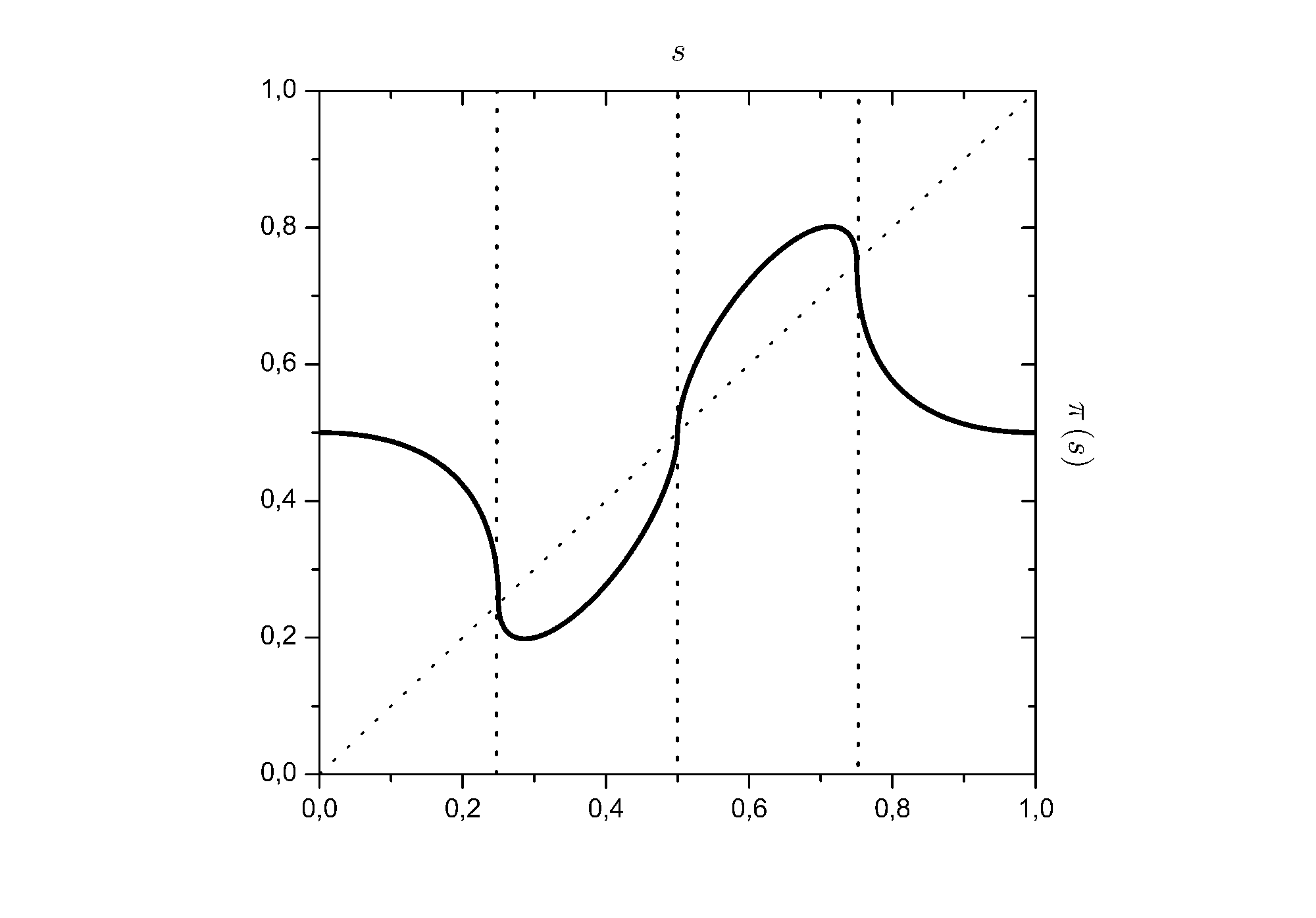
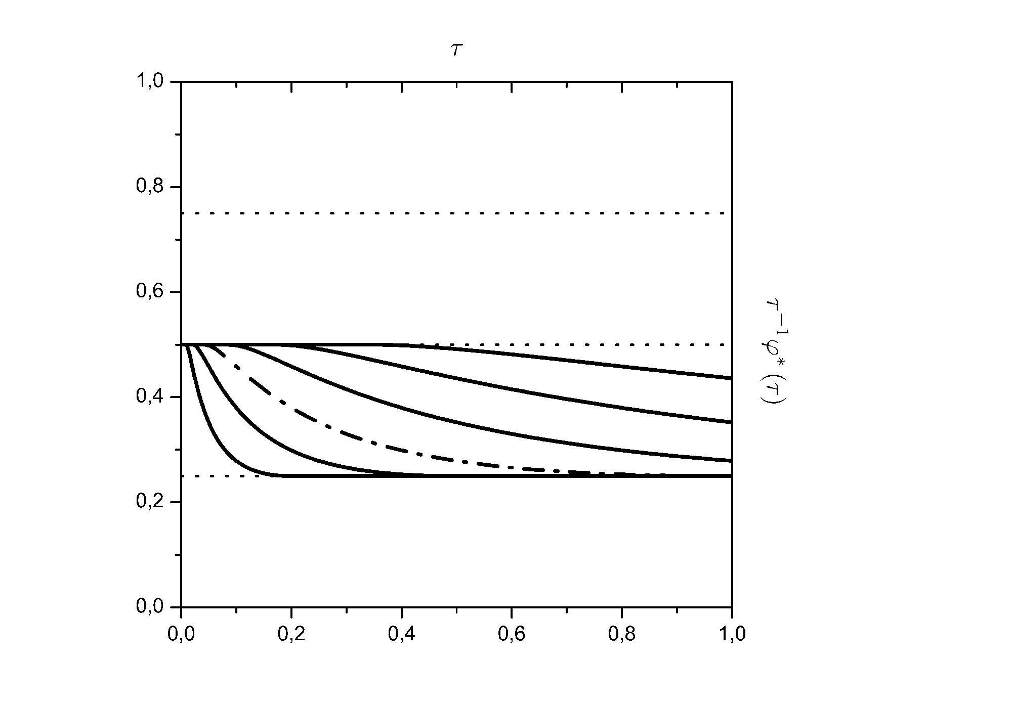
Figure 2.2. In the above figures we give an example to show the effects of integrability on stable and unstable points. Consider the urn function $\pi\left(s\right)=s+\mathbb{I}_{\left\{s\in\left[01/4\right]\right\}}(1/4-s)^{1/2}-\mathbb{I}_{\left\{s\in\left(1/4,1/2\right]\right\}}(1/4-s)^{1/2}(s-1/2){}^{1/2}+\,\mathbb{I}_{\left\{s\in\left(1/2,3/4\right]\right\}}(1/2-s)^{1/2}(s-3/4)^{1/2}-\mathbb{I}_{\left\{s\in\left(3/4,1\right]\right\}}(s-3/4)^{1/2}$ in the interval $s\in\left[1/4,1/2\right]$, then we have $F_{\pi}\left(s,u\right)=\left[2\arcsin\left(\sqrt{4z-1}\right)\right]_{u}^{s}$ and $\theta_{i}^{*}=\exp(-\pi)$. By Corollary 7 we find that the family of trajectories ending in $s_{i}^{\dagger}=1/2$ is ${\scriptstyle{\textstyle 4\tau^{-1}\varphi_{\tau}^{*}=\mathbb{I}_{\left\{\tau\in\left[1,t\right]\right\}}+2\,\mathbb{I}_{\left\{\tau\in\left[0,e^{-\pi}t\right]\right\}}}+{\textstyle\left[1+\sin^{2}\left(\frac{1}{2}\log\left(t/\tau\right)\right)\right]\mathbb{I}_{\left\{\tau\in\left[e^{-\pi}t,t\right]\right\}}}}$ for $t\in\left[0,1\right]$, while for each $s\in\left(1/4,1/2\right]$ we have $\tau_{s,i}^{*}=\exp[2\arcsin\left(\sqrt{4s-1}\right)-\pi]$ and $4\tau^{-1}\varphi_{\tau}^{*}=[1+\sin^{2}(\frac{1}{2}\log(\tau_{s,i}^{*}/\tau))]\,\mathbb{I}_{\{\tau\in(\tau_{s,i}^{*},1]\}}+2\,\mathbb{I}_{\{\tau\in[0,\tau_{s,i}^{*}]\}},$ with $\lim_{s\rightarrow s_{i}^{\dagger}}\tau_{s,i}^{*}=\theta_{i}^{*}$ as expected. The urn function and some zero-cost trajectories in $K_{\pi,1}\cup\partial K_{\pi,1}=\left[1/4,\,1/2\right]$ are shown in lower figure, with $s=\frac{1}{4}\left[1+\sin^{2}\left(\frac{1}{2}\log\left(k\right)\right)\right]$, $k\in\left\{2,\,4,\,8\right\}$ and with $t=\left\{1/8,\,1/2,\,1\right\}$. The dash-dotted line is the critical trajectory with $t=1$.

It is an interesting result that no trajectory with $\lim_{\tau\rightarrow 0}\left(\varphi_{\tau}/\tau\right)\notin\partial C_{\pi}$ can be optimal if $a_{\pi,i}\neq 0$, not even if we chose $\varphi_{1}$ to be in a set of stable equilibrium like downcrossings (ie, $\varphi_{1}\in C_{\pi}\left(+,-\right)$). We can interpret this result in terms of time spent in a given state: it seems that a process starting with initial conditions $m^{-1}X_{n,m}\notin\partial C_{\pi}$ concentrates its mass in the neighborhood of the points of convergence in times that are of order $o\left(n\right)$, and only those that are in the neighborhood of unstable points can remain there for times $O\left(n\right)$, eventually reaching the stable points according to the mechanism suggested by Corollaries 6 and 7.

2.2.2. A comment on moderate deviations

The above formulas for optimal trajectories are of particular interest, since represent a first step to deal with the much richer problem of moderate deviations, ie, to compute limits of the kind

(2.24) $$\phi_{\left\{\sigma_{n}\right\}}\left(s_{1},s_{2}\right)=\lim_{n\rightarrow\infty}\sigma{}_{n}^{-1}\log\mathbb{P}\left(n^{-1}X_{n,n}\in\left(s_{1},s_{2}\right)\right)$$

for some $\sigma_{n}=o\left(n\right)$, $s\in\left[\,\inf\,C_{\pi},\,\sup\,C_{\pi}\right]$. To illustrate how this can be obtained we provide the following argument. Let $u_{\tau,s}^{*}$ be an optimal trajectory ending in $s\in K_{\pi,i}$ (ie, $u_{1,s}^{*}=s$). Since any finite deviation from this trajectory has an exponential cost on a time scale $O\left(n\right)$, the probability mass current can move along these trajectories only. Moreover, Corollaries 6 and 7 guarantee uniqueness of the solutions and $u_{\tau,s_{1}}^{*}<u_{\tau,s}^{*}<u_{\tau,s_{2}}^{*}$ for any $\tau\in\left(0,1\right]$ and $s_{1}<s<s_{2}$. Hence, we find that the probability current passing through $\left(u_{\tau,s_{1}}^{*},u_{\tau,s_{2}}^{*}\right)$ is constant for $\tau>0$,

(2.25) $$\mathbb{P}\left(x_{n,\tau n}\in\left(u_{\tau,s_{1}}^{*},u_{\tau,s_{2}}^{*}\right)\right)=\mathbb{P}\left(x_{n,n}\in\left(s_{1},s_{2}\right)\right),\,\tau\in\left(0,1\right].$$

Then, let $\tau\left(s_{i},\epsilon\right)$ such that $u_{\tau\left(s_{i},\epsilon\right)}^{*}=s_{i}+\epsilon$ and let consider the case $\tau\left(s_{1},\epsilon\right)>\tau\left(s_{2},\epsilon\right)$ for $s_{1}<s_{2}$. Corollaries 6 and 7 also guarantee invertibility of the zero-cost trajectories, then we can write

(2.26) $$\mathbb{P}\left(x_{n,n}\in\left(s_{1},s_{2}\right)\right)=\mathbb{P}\left(x_{n,\tau\left(s_{1},\epsilon\right)n}-s_{i}^{*}<\epsilon\right)-\mathbb{P}\left(x_{n,\tau\left(s_{2},\epsilon\right)n}-s_{i}^{*}<\epsilon\right).$$

Given that $\mathbb{P}\left(x_{n,k}\in\left(\alpha,\beta\right)\right)=\mathbb{P}\left(x_{k,k}\in\left(\alpha,\beta\right)\right)$, the problem of computing $\mathbb{P}\left(x_{n,n}\in\left(s_{1},s_{2}\right)\right)$ is reduced to that of computing $\mathbb{P}\left(x_{n,n}-s_{i}^{*}<\epsilon\right)$ for some arbitrary small $\epsilon>0$. For $\left(s_{1},s_{2}\right)\subseteq K_{\pi,i}$ a martingale analysis suggests the conjecture that $\phi_{\left\{n^{\nu}\right\}}\left(s_{1},s_{2}\right)=0$ for any $\nu\in\left(0,1\right)$, and that $\phi_{\left\{\log n\right\}}\left(s_{1},s_{2}\right)=1-\left[\partial_{s}\pi\left(s\right)\right]_{s=s_{i}^{*}}$.

2.3. Cumulant Generating Function.

Except the fact that $\phi\left(s\right)<0$, for $s\in\left[z_{-}^{*},\inf C_{\pi}\right)$ or $s\in\left(\sup\,C_{\pi},z_{+}^{*}\right]$ we couldn’t extract more informations on the shape of $\phi\left(s\right)$ from its variational representation, because in these cases the variational problem can’t be simplified by Lemma 18, see Section 3.2.2. Anyway, the existence of $\phi$ proved in Theorem 4 introduces some critical simplifications that allows to approach the problem using analysis, provided that $\pi$ obeys to some additional regularity conditions. For example, we can prove the convexity of $-\phi\left(s\right)$, $s\in\left[z_{-}^{*},\inf C_{\pi}\right)$, or $s\in\left(\sup\,C_{\pi},z_{+}^{*}\right]$ in case $\pi$ is invertible on the same intervals and the inverse functions

(2.27) $$\pi_{-}^{-1}:\,\left[\pi\left(z_{-}^{*}\right),\pi(\inf C_{\pi})\right)\rightarrow\,\left[\,z_{-}^{*},\,\inf C_{\pi}\right),$$

(2.28) $$\pi_{+}^{-1}:\left(\pi(\sup\,C_{\pi}),\pi\left(z_{+}^{*}\right)\right]\rightarrow\left(\sup\,C_{\pi},z_{+}^{*}\right],$$

are absolutely continuous Lipschitz functions. Such result can be obtained by analyzing the scaling of the Cumulant Generating Function (CGF)

(2.29) $$\psi\left(\lambda\right):=\lim_{n\rightarrow\infty}n^{-1}\log\mathbb{E}\left(e^{\lambda X_{n,n}}\right),\ \lambda\in\left(-\infty,\infty\right).$$

First, notice that Theorem 4 implies that $\psi$ is well defined [DZ1998]. Then, let $-\hat{\phi}\left(s\right)=\mathrm{conv\left(-\phi\left(s\right)\right)}$ be the convex envelope of $-\phi\left(s\right)$ for $s\in\left[0,1\right]$. By Theorem 4 and Corollary 5 it follows that $\hat{\phi}\left(s\right)=0$ when $s\in\left[\,\inf\,C_{\pi},\,\sup\,C_{\pi}\right]$ and $\hat{\phi}\left(s\right)<0$ otherwise. In addition, it holds that

Definition 8.

Let $\hat{\phi}_{-}:\left[z_{-}^{*},\inf C_{\pi}\right)\rightarrow\left(-\infty,0\right]$, $\hat{\phi}_{+}:\left(\sup\,C_{\pi},z_{+}^{*}\right]\rightarrow\left(-\infty,0\right]$ such that $\hat{\phi}\left(s\right)=\hat{\phi}_{-}\left(s\right)$ when $s\in\left[z_{-}^{*},\inf C_{\pi}\right)$ and $\hat{\phi}\left(s\right)=\hat{\phi}_{+}\left(s\right)$ when $s\in\left(\sup\,C_{\pi},z_{+}^{*}\right]$. Also define $\psi_{-}:\left(-\infty,0\right]\rightarrow\left(-\infty,0\right]$, $\psi_{+}:\left[0,\infty\right)\rightarrow\left[0,\infty\right)$ such that $\psi\left(\lambda\right)=\psi_{-}\left(\lambda\right)$ when $\lambda\in\left(-\infty,0\right]$ and $\psi\left(\lambda\right)=\psi_{+}\left(\lambda\right)$ when $\lambda\in\left[0,\infty\right)$. One can show that $-\hat{\phi}_{-}$ and $-\hat{\phi}_{+}$ are the Frenchel-Legendre transforms of $-\psi_{-}$ and $-\psi_{+}$ respectively:

(2.30) $$\hat{\phi}_{-}\left(s\right)=\inf_{\lambda\in\left(-\infty,0\right]}\left\{\lambda s+\psi_{-}\left(\lambda\right)\right\},\>\hat{\phi}_{+}\left(s\right)=\inf_{\lambda\in\left[0,\infty\right)}\left\{\lambda s+\psi_{+}\left(\lambda\right)\right\}.$$

Since the existence of $-\hat{\phi}$ implies the existence of $\psi$ for every $\pi\in\mathcal{U}$, while its convexity ensures that $\psi\in\mathcal{AC}$, we have enough informations to approach $\psi$ by analytic methods. Here we show that the Cumulant Generating Function satisfies the non-linear implicit ODE,

(2.31) $$\pi\left(\partial_{\lambda}\psi\left(\lambda\right)\right)={\textstyle\frac{e^{\psi\left(\lambda\right)}-1}{e^{\lambda}-1}},$$

for any $\lambda$. We stress that the CGF satisfies the above equation for all $\pi\in\mathcal{U}$, but any information would be hard to be extracted if $\pi$ is not invertible at least on $\left[z_{-}^{*},\inf C_{\pi}\right)$ and $\left(\sup\,C_{\pi},z_{+}^{*}\right]$. If this is the case, then the following theorem provides the Cauchy problems for $\psi_{-}$ and $\psi_{+}$:

Theorem 9.

Let $\pi\in\mathcal{U}$ be invertible on $\left[z_{-}^{*},\inf C_{\pi}\right)$, and denote by $\pi_{-}^{-1}:\left[\pi\left(z_{-}^{*}\right),\pi(\inf C_{\pi})\right)\rightarrow\left[z_{-}^{*},\inf C_{\pi}\right)$ its inverse. If $\pi_{-}^{-1}$ is $\mathcal{AC}$ and Lipschitz, then for $\lambda\in\left(-\infty,0\right)$ we have $\psi\left(\lambda\right)=\psi_{-}\left(\lambda\right)$, with $\psi_{-}\left(\lambda\right)$ solution to the Cauchy problem

(2.32) $$\partial_{\lambda}\psi_{-}\left(\lambda\right)=\pi_{-}^{-1}\left({\textstyle\frac{e^{\psi_{-}\left(\lambda\right)}-1}{e^{\lambda}-1}}\right),\,\lim_{\lambda\rightarrow 0^{-}}\,\partial_{\lambda}\psi_{-}\left(\lambda\right)=\pi_{+}\left(\inf\,C_{\pi}\right),\,\lim_{\lambda\rightarrow-\infty}\,\partial_{\lambda}\psi_{-}\left(\lambda\right)=z_{-}^{*},$$

Let $\pi$ be invertible on $\left(\sup\,C_{\pi},z_{+}^{*}\right]$, with $\pi_{+}^{-1}:\left(\pi(\sup\,C_{\pi}),\pi\left(z_{+}^{*}\right)\right]\rightarrow\left(\sup\,C_{\pi},z_{+}^{*}\right]$ its inverse function. If $\pi_{+}^{-1}$ is $\mathcal{AC}$ and Lipschitz, then for $\lambda\in\left(0,\infty\right)$ we have $\psi\left(\lambda\right)=\psi_{+}\left(\lambda\right)$, with $\psi_{+}\left(\lambda\right)$ solution to the Cauchy problem

(2.33) $$\partial_{\lambda}\psi_{+}\left(\lambda\right)=\pi_{+}^{-1}\left({\textstyle\frac{e^{\psi_{+}\left(\lambda\right)}-1}{e^{\lambda}-1}}\right),\,\lim_{\lambda\rightarrow 0^{+}}\,\partial_{\lambda}\psi_{+}\left(\lambda\right)=\pi_{+}\left(\sup\,C_{\pi}\right),\,\lim_{\lambda\rightarrow\infty}\,\partial_{\lambda}\psi_{+}\left(\lambda\right)=z_{+}^{*}.$$

A unique global solution exists for both Cauchy problems (2.32), (2.33), it is $\mathcal{AC}$ and has continuous first derivative.

Although the above result is obtained for urn functions belonging to a subset of $\mathcal{U}$ we consider it of special importance from the applicative side as it allows to explicitly compute $\phi$ (at least numerically) in those intervals of $s$ where $\phi$ is nontrivial, thus providing a substantial improvement of Corollary 5.

Another trivial but potentially useful application is the inverse problem of deciding weather a given function $f$ can be the rate function of some urn process. Since $-\hat{\phi}\left(s\right)$ is convex by definition, then $\psi\left(\lambda\right)=\hat{\phi}\left(\partial_{\lambda}\psi\right)-\lambda\partial_{\lambda}\psi$, from which follows that $\lambda\left(s\right)=-\partial_{s}\hat{\phi}\left(s\right)$ and $\psi\left(\lambda\left(s\right)\right)=\hat{\phi}\left(s\right)-s\partial_{s}\hat{\phi}\left(s\right)$. If $-\phi$ is convex, then obviously $\phi=\hat{\phi}$ and we can state the following corollary:

Corollary 10.

Let $f:\left[0,1\right]\rightarrow\left(-\infty,0\right]$ be a bounded and concave $\mathcal{AC}$ function, and define the function $\pi_{f}$ as follows:

(2.34) $$\pi_{f}\left(s\right)={\textstyle{\displaystyle\frac{e^{f\left(s\right)-s\,\partial_{s}f\left(s\right)}-1}{e^{-\partial_{s}f\left(s\right)}-1}}},\,s\in\left[0,1\right].$$

If the function $f$ is such that $\pi_{f}\in\mathcal{U}$ and $f\left(0\right)=\log(1-\pi_{f}\left(0\right))$, $f\left(1\right)=\log(\pi_{f}\left(1\right))$ then the limit $\phi$ defined in Eq. (2.12) for an urn process with urn function $\pi_{f}$ is $\phi=f$.

We believe that such result could find useful applications in those stochastic approximation algorithms for which the process is required to satisfy some given LDP. Notice that these results quite immediately imply the convexity of $-\phi$ since if the cumulants $-\psi_{-}$ and $-\psi_{+}$ have continuous first derivatives their Frenchel-Legendre transforms $-\hat{\phi}_{-}$, $-\hat{\phi}_{+}$ must be strictly convex, with $\hat{\phi}_{-}=\phi_{-}$ and $\hat{\phi}_{+}=\phi_{+}$.

Corollary 11.

Let $\pi\in\mathcal{U}$ invertible on $\left[z_{-}^{*},\inf C_{\pi}\right)$, and denote by $\pi_{-}^{-1}:\left[\pi\left(z_{-}^{*}\right),\pi(\inf C_{\pi})\right)\rightarrow\left[z_{-}^{*},\inf C_{\pi}\right)$ its inverse function. If $\pi_{-}^{-1}$ is $\mathcal{AC}$ and Lipschitz, then $\phi_{-}$ is in $\mathcal{AC}$, is strictly concave on $\left[z_{-}^{*},\inf C_{\pi}\right)$, and strictly increasing from $\log\bar{\pi}\left(z_{-}^{*}\right)$ to $0$. Let $\pi$ be invertible on $\left(\sup\,C_{\pi},z_{+}^{*}\right]$, with inverse function $\pi_{+}^{-1}:\left(\pi(\sup\,C_{\pi}),\pi\left(z_{+}^{*}\right)\right]\rightarrow\left(\sup\,C_{\pi},z_{+}^{*}\right]$. If $\pi_{+}^{-1}$ is $\mathcal{AC}$ and Lipschitz, then $\phi_{+}$ is in $\mathcal{AC}$, it is strictly concave on $\left(\sup\,C_{\pi},z_{+}^{*}\right]$, and strictly decreasing from $0$ to $\log\pi\left(z_{+}^{*}\right)$.

Linear urns and the Bachi-Pal Model

The last topic we present is the application to the Baghi-Pal model, a widely investigated model due to its relevance in studying branching phenomena and random trees (see [Pem2007, Mam2003, Mam2008, JK1977, KMR2000] for some reviews). Consider an urn with black and white balls: at each step a ball is extracted uniformly from the urn and some new balls are added or discarded according to the square matrix

(2.35) $$A:=\left(\begin{array}[]{cc}a_{11}&a_{12}\\ a_{21}&a_{22}\end{array}\right),$$

with $a_{ij}\in\mathbb{Z}$, such that if the extraction resulted in a black ball we add $a_{11}$ black balls and $a_{12}$ white balls, otherwise we add $a_{21}$ black balls and $a_{22}$ white balls. If $a_{11}+a_{12}=a_{21}+a_{22}=M$, then the number of balls increases (ore decreases) by some deterministic rate $M$ and the urn is said to be balanced, if $M>0$ the urn is said to be also tenable.

Beside the many applicative aspects, our interest araises from the fact that this is the first nontrivial model for which some large deviations results have been obtained. In [FGP2005, FDP2006] the so-called subtractive case (negative diagonal entries) is fully analyzed by purely analytic methods, obtaining an explicit characterization of the rate function and other important results. Another LDP study on linear urns involving more probabilistic techniques has been provided by Bryc et Al. [BMS2009]. In this paper they consider a process with urn function $\pi\left(s\right)=1-s/\alpha$, $\alpha\in\left(1,\infty\right)$, giving an expression for the Cumulant Generating Function and other related results.

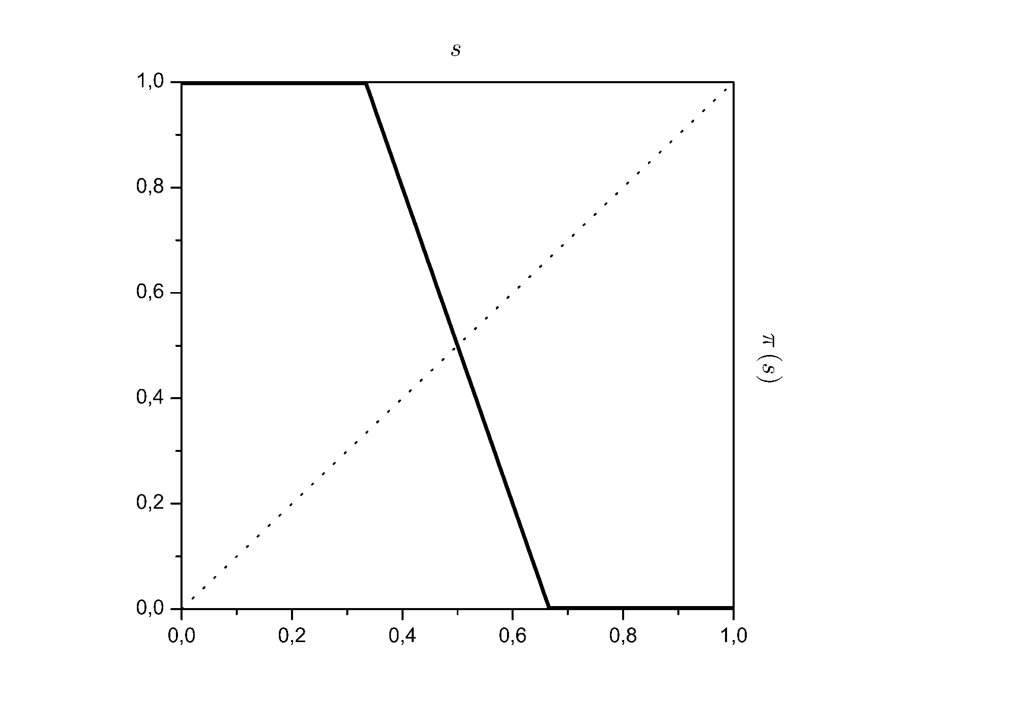
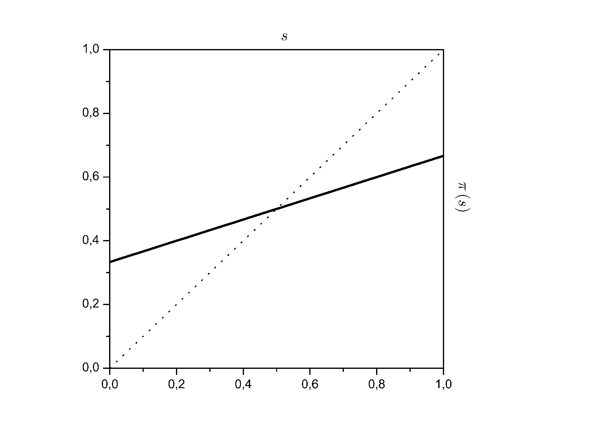
Figure 2.3. Urn functions from Eq.s (2.39) and (2.40) of Bagchi-Pal models for $a_{11}=a_{22}=-1$, $a_{21}=a_{12}=2$ (upper figure) and $a_{11}=a_{22}=2$, $a_{21}=a_{12}=1$ (lower figure). The first one is a subtractive urn of the kind considered in [FGP2005], while the second is an additive and tenable urn.

Let show that the above model is equivalent to a linear urn function $\pi\left(s\right)=s_{0}+b\left(s-s_{0}\right)$ provided that $A$ fulfills some self-consistency conditions. Let $B_{k}$ and $W_{k}$ be the number of black and withe balls of a Bagchi-Pal urn at time $k$, let $T_{k}=B_{k}+W_{k}$ be the total number of balls and

(2.36) $$A=\left(\begin{array}[]{cc}a_{11}&M-a_{11}\\ M-a_{22}&a_{22}\end{array}\right)$$

the reinforcement matrix, where we used the balancing constraint $a_{11}+a_{12}=a_{21}+a_{22}=M$. Since the balancing ensures that $T_{k}=\left(B_{0}+W_{0}\right)+Mk$, we can rescale $k\rightarrow k-M^{-1}\left(B_{0}+W_{0}\right)$ and consider $k\geq m=M^{-1}\left(B_{0}+W_{0}\right)$, $T_{k}=Mk$. Then, define the variable

(2.37) $$X_{n,k}=\frac{B_{k}-\left(M-a_{22}\right)k}{a_{11}+a_{22}-M},$$

with $a_{11}+a_{22}-M\neq 0$: we can show that the process $\left\{X_{n,k}:m\leq k\leq n\right\}$ defined by the urn function $\pi\left(s\right)=s_{0}+b\left(s-s_{0}\right)$, with

(2.38) $$s_{0}=\frac{a_{22}-M}{2M-a_{11}-a_{22}},\,b=\frac{a_{11}+a_{22}}{M}-1,\,X_{n,m}=\frac{B_{0}-\left(M-a_{22}\right)m}{a_{11}+a_{22}-M}.$$

is equivalent to a Bagchi-Pal model with reinforcement matrix

(2.39) $$A=M\left(\begin{array}[]{cc}b+s_{0}\left(1-b\right)&\left(1-s_{0}\right)\left(1-b\right)\\ s_{0}\left(1-b\right)&1-s_{0}\left(1-b\right)\end{array}\right).$$

Since the Bagchi-Pal model usually considers an integer reinforcement matrix, we need $M$, $s_{0}$, $b$, $m$ such that both $B_{0}+W_{0}$ and the elements of $A$ are integers. If $a_{12}=a_{21}=0$ we recover the Polya Urn ($b=1$), while we obviously have to discard the case $a_{11}=a_{21}$ (deterministic evolution of the urn: $a_{11}+a_{22}-M=0$). Usually some tenability conditions are assumed which ensures that the process can’t be stopped, ie, that the total number of balls is deterministic and always growing ($M>0$), that $a_{12}\geq 0$, $a_{21}\geq 0$ and if $a_{11}<0$ then $\left(W_{0}/a_{11}\right),\left(a_{21}/a_{11}\right)\in\mathbb{Z}$, if $a_{22}<0$ then $\left(B_{0}/a_{22}\right),\left(a_{12}/a_{22}\right)\in\mathbb{Z}$. The last two conditions ensure that only balls of the same color of that drawn can be removed from the urn: this prevents from stopping the process by impossible removals.

According to the above discussion, and considering that $B_{0}/m\in\left[0,1\right]$, it is possible to show that the general urn function describing the balanced Baghi-Pal urns is

(2.40) $$\pi\left(s\right)=\mathbb{I}_{\left\{s_{0}+b\left(s-s_{0}\right)\geq 1\right\}}+\left(s_{0}+b\left(s-s_{0}\right)\right)\mathbb{I}_{\left\{0<s_{0}+b\left(s-s_{0}\right)<1\right\}}.$$

As example, the subtractive urn $a_{11}=a_{22}=-1$, $a_{12}=a_{21}=2$ is described by the urn function (see Figure 2.3)

(2.41) $$\pi\left(s\right)=\mathbb{I}_{\left\{s\in\left[0,1/3\right)\right\}}+\left(2-3s\right)\mathbb{I}_{\left\{s\in\left[1/3,2/3\right]\right\}}.$$

In the following we provide a complete characterization of the CGF for the case of linear urn, which also includes all cases of the balanced Bagchi-Pal models. We only consider linear urn functions with $a>0$ and $a+b<1$ to exclude the “trivial” cases with $\pi\left(0\right)=0$ and $\pi\left(1\right)=1$, for which by Corollary 5 we would find $\phi\left(s\right)=0$ for any $s\in\left[0,1\right]$, and for which we can even compute the optimal trajectories by Corollaries 6, 7.

Corollary 12.

Let $\pi$ be as in Eq. (2.40) with $a>0$ and $a+b<1$, $\psi$ as in Eq. (2.29) and define the function

(2.42) $$B\left(\alpha,\beta;x_{1},x_{2}\right)=\int_{x_{1}}^{x_{2}}dt\,\left(1-t\right)^{\alpha-1}t^{\beta-1}.$$

Then, for $\lambda>0$ we have $\psi=\psi_{+}$, with

(2.43) $$\psi_{+}\left(\lambda\right)=\psi_{+}\left(\lambda;b<0\right)\mathbb{I}_{\left\{b<0\right\}}+\psi_{+}\left(\lambda;b>0\right)\mathbb{I}_{\left\{b>0\right\}},$$

where $\psi_{+}\left(\lambda;b>0\right)$, $\psi_{+}\left(\lambda;b<0\right)$ are given by the expressions

(2.44) $$e^{-\psi_{+}\left(\lambda;b>0\right)}=1-{\textstyle\frac{a}{b}}e^{-\frac{a}{b}\lambda}\left({\textstyle 1-e^{-\lambda}}\right)^{\frac{1}{b}}B\left({\textstyle{\textstyle\frac{a}{b}},\frac{b-1}{b};1-e^{-\lambda},1}\right),$$

(2.45) $$e^{-\psi_{+}\left(\lambda;b<0\right)}=1+{\textstyle\frac{a}{b}}e^{-\frac{a}{b}\lambda}\left({\textstyle 1-e^{-\lambda}}\right)^{\frac{1}{b}}B\left({\textstyle{\textstyle{\textstyle\frac{a}{b}},\frac{b-1}{b};0,\,}1-e^{-\lambda}}\right).$$

If $\lambda<0$ we have instead $\psi=\psi_{-}$, with

(2.46) $$\psi_{-}\left(\lambda\right)=\psi_{-}\left(\lambda;b<0\right)\mathbb{I}_{\left\{b<0\right\}}+\psi_{-}\left(\lambda;b>0\right)\mathbb{I}_{\left\{b>0\right\}},$$

where $\psi_{-}\left(\lambda;b>0\right)$, $\psi_{-}\left(\lambda;b<0\right)$ are given by

(2.47) $$e^{-\psi_{-}\left(\lambda;b>0\right)}=1+{\textstyle\frac{a}{b}}e^{-\frac{1-a+b}{b}\lambda}\left({\textstyle 1-e^{\lambda}}\right)^{\frac{1}{b}}B\left({\textstyle\frac{1-a}{b},\frac{b-1}{b};1-e^{\lambda},1}\right),$$

(2.48) $$e^{-\psi_{-}\left(\lambda;b<0\right)}=1-{\textstyle\frac{a}{b}}e^{-\frac{1-a+b}{b}\lambda}\left({\textstyle 1-e^{\lambda}}\right)^{\frac{1}{b}}B\left({\textstyle\frac{1-a}{b},\frac{b-1}{b};0,1-e^{\lambda}}\right).$$

An intriguing property of the above solution is that if $b>0$ then $\psi$ is non-analytic at $\lambda\rightarrow 0^{-}$($\lambda\rightarrow 0^{+}$). We can see this, for example, from the expression of $\psi_{-}\left(\lambda;b>0\right)$: expanding for small $\lambda$ we find a non vanishing therm $O\left(\lambda^{1/b}\log\left(\lambda\right)\right)$ if $1/b\in\mathbb{N}$ and $O\left(\lambda^{1/b}\right)$ if $1/b\notin\mathbb{N}$, which implies that the derivatives of order $\left\lceil 1/b\right\rceil$ and higher are singular in $\lambda=0$. The singularity disappears for $b<0$.

This behavior is not observed in case of subtractive urns for which the rate function is always analytic in $\lambda=0$, as first noticed in [FGP2005]. This is not surprising since these urns are affine to the case $b<0$ for which we also observe a regular solution. Notice that a non-analytic point in $\lambda=0$ implies divergent cumulants from $\left\lceil 1/b\right\rceil$ order onwards. Moreover, if $b>1/2$ the shape of $\phi\left(s\right)$ around its peak is not even Gaussian anymore, since we find a divergent second cumulant $\partial_{\lambda}^{\,2}\,\psi\left(\lambda\right)=O\left(\lambda^{-\gamma}\right)$ with $\gamma=2-1/b>0$. If $b=1/2$ we a logarithmic divergence of $\partial_{\lambda}^{\,2}\,\psi\left(\lambda\right)$ is observed as expected from the moment analysis of the Bagchi-Pal model (see [Mam2008] for a review).

3. Proofs.

In this section we collected most of the proofs and technical features of the present work. The proofs are presented in the order they appeared in the previous section. We will first deal with the Sample-Path Large Deviation Principle, then the entropy of the event $\left\{X_{n}=\left\lfloor sn\right]\right\}$ and, finally, with the Cumulant generating function. We assume that all random variables and processes are defined in a common probability space $\left(\Omega,\mathcal{F},\mathbb{P}\right)$.

3.1. Sample-Path Large Deviation Principle.

Here we prove the existence of Sample-Path LDPs for $\chi_{n}$ using some standard Large Deviation tools, such as Mogulskii Theorem and the Varadhan Integral Lemma.

Before we get into the core of this, we recall that $\left\|\varphi\right\|:=\sup_{\tau\in\left[0,1\right]}\left|\varphi_{\tau}\right|$ is the usual supremum norm, and we consider the metric space $\left(\mathcal{Q},\,\left\|\cdot\right\|\right)$, with $\mathcal{Q}$ defined in Eq. (2.2). Note that $\mathcal{Q}$ is compact with respect to the supremum norm topology. Moreover, since by definition $\left\|\varphi\right\|\leq 1$ for any $\varphi\in\mathcal{Q}$ we trivially find that $\mathcal{Q}\subset L_{\infty}\left(\left[0,1\right]\right)$.

3.1.1. Change of measure.

We need a variational representation for the rate function of $\chi_{n}$ in terms of sample paths. Let $\varphi:=\left\{\varphi_{\tau}:\tau\in\left[0,1\right]\right\}$, and define

(3.1) $$\mathcal{Q}_{n}:=\{\varphi:\,\varphi_{\tau}=\frac{1}{n}\sum_{1\leq i\leq\left\lfloor n\tau\right\rfloor}\theta_{i}+(\tau-n^{-1}\left\lfloor n\tau\right\rfloor)\,\mathbf{\theta}_{\left\lfloor n\tau\right\rfloor}\,,\,\theta_{i}\in\left\{0,1\right\}\}.$$

The above set is the support of $\chi_{n}$ for $n<\infty$: note that $\mathcal{Q}_{n}\subset\mathcal{Q}$ for all $n$. We also introduce the following notation:

(3.2) $$Y_{n,k}\left(\varphi\right):=n\varphi_{k/n},\,\delta Y_{n,k}\left(\varphi\right):=n\left(\varphi_{\left(k+1\right)/n}-\varphi_{k/n}\right),$$

Then, let $\varphi\in\mathcal{\mathcal{Q}}_{n}$: by Eq. (1.3) we can write the sample-path probability $\mathbb{P}\left(\chi_{n}=\varphi\right)$ in terms of $\varphi$ as follows:

(3.3) $$\mathbb{P}\left(\chi_{n}=\varphi\right)=\prod_{1\leq k\leq n-1}\pi\left(Y_{n,k}\left(\varphi\right)/k\right)^{\delta Y_{n,k}\left(\varphi\right)}\bar{\pi}\left(Y_{n,k}\left(\varphi\right)/k\right)^{1-\delta Y_{n,k}\left(\varphi\right)}.$$

Our first step is to prove Theorem 1 under the additional assumption that $\pi\left(s\right)\in\left(0,1\right)$ for all $s\in\left[0,1\right]$. In this case the proof can be obtained by straight applications of the Mogulskii Theorem, the Varadhan Integral Lemma and the following two lemmas.

Let $S_{\pi}:\mathcal{Q}\rightarrow\left(-\infty,0\right]$ be as in Eq. (2.5). The first lemma shows the continuity of $S_{\pi}$ with respect to the supremum norm for any compact subset of $\mathcal{\mathcal{Q}}$ and any $\pi\in\mathcal{U}$, $\pi\in\left(0,1\right)$. The second gives an approximation argument to the functional $S_{\pi}$ for the entropy of the event $\left\{\chi_{n}=\varphi\right\}$ when $\varphi\in\mathcal{\mathcal{Q}}_{n}$.

Lemma 13.

Assume $\pi\in\mathcal{U}$ and $\pi\left(s\right)\in\left(0,1\right)$ for all $s\in\left[0,1\right]$. The functional $S_{\pi}:\mathcal{Q}\rightarrow\left(-\infty,0\right]$ is continuous on the metric space $\left(\mathcal{\mathcal{Q}},\,\left\|\cdot\right\|\right)$. Moreover, a function $W_{\pi}:\left[0,1\right]\rightarrow\left[0,\infty\right)$ exists such that $\lim{}_{s\rightarrow 0}W_{\pi}\left(s\right)=0$ and $\left|S_{\pi}\left[\varphi\right]-S_{\pi}\left[\eta\right]\right|\leq W_{\pi}\left(\left\|\varphi-\eta\right\|\right)$, $\forall\varphi,\eta\in\mathcal{Q}$.

Proof.

Take any $\varphi,\eta\in\mathcal{Q}$. By definition of $S_{\pi}$, we can rearrange the terms as follows

(3.4) $$S_{\pi}\left[\varphi\right]-S_{\pi}\left[\eta\right]=\int_{\tau\in\left[0,1\right]}d\varphi_{\tau}\,\log\pi\left(\varphi_{\tau}/\tau\right)-\int_{\tau\in\left[0,1\right]}d\eta_{\tau}\,\log\pi\left(\eta_{\tau}/\tau\right)+\\ +\int_{\tau\in\left[0,1\right]}d\tilde{\varphi}_{\tau}\,\log\bar{\pi}\left(\varphi_{\tau}/\tau\right)-\int_{\tau\in\left[0,1\right]}d\tilde{\eta}_{\tau}\,\log\bar{\pi}\left(\eta_{\tau}/\tau\right),$$

where we used the notation $\tilde{\varphi}=\tau-\varphi$, $\tilde{\eta}=\tau-\eta$. Let us first consider $\log\pi\left(s\right)$: by definition of the set $\mathcal{U}$ and the assumption that $\pi\in\left(0,1\right)$ we have that $\left\|\log\pi\right\|<\infty$, and that $\left|\log\pi\left(x+\delta\right)-\log\pi\left(x\right)\right|\leq f\left(\left|\delta\right|\right)$ and $\lim_{\epsilon\rightarrow 0}\epsilon\int_{\epsilon}^{1}dz\,f\left(z\right)/z^{2}=0$. Then we can write

(3.5) $$\int_{\tau\in\left[0,1\right]}d\varphi_{\tau}\,\log\pi\left(\varphi_{\tau}/\tau\right)-\int_{\tau\in\left[0,1\right]}d\eta_{\tau}\,\log\pi\left(\eta_{\tau}/\tau\right)=\\ =\int_{\tau\in\left[0,1\right]}d\varphi_{\tau}\,\left[\log\pi\left(\varphi_{\tau}/\tau\right)-\log\pi\left(\eta_{\tau}/\tau\right)\right]+\int_{\tau\in\left[0,1\right]}d\left(\varphi_{\tau}-\eta_{\tau}\right)\,\log\pi\left(\varphi_{\tau}/\tau\right).$$

By the uniform continuity condition one has $\left|\log\pi\left(\varphi_{\tau}/\tau\right)-\log\pi\left(\eta_{\tau}/\tau\right)\right|\leq f\left(\left|\varphi_{\tau}-\eta_{\tau}\right|/\tau\right)$. Moreover, since $\varphi_{\tau}\leq\tau$ and $\eta_{\tau}\leq\tau$, we have

(3.6) $$\left|\varphi_{\tau}-\eta_{\tau}\right|\leq\min\left\{\tau,\,\left\|\varphi-\eta\right\|\right\},$$

and $d\varphi_{\tau}\leq d\tau$. Then, if we define $s^{-1}H_{f}\left(s\right):=\int_{s}^{1}dz\,f\left(z\right)/z^{2}$ the first integral can be bounded as follows

(3.7) $$\int_{\tau\in\left[0,1\right]}d\varphi_{\tau}\,\left|\log\pi\left(\varphi_{\tau}/\tau\right)-\log\pi\left(\eta_{\tau}/\tau\right)\right|\leq\left\|\bar{\pi}\right\|^{-1}H_{f}\left(\left\|\varphi-\eta\right\|\right),$$

while for the second we get

(3.8) $$\int_{\tau\in\left[0,1\right]}d\left(\varphi_{\tau}-\eta_{\tau}\right)\,\left|\log\pi\left(\varphi_{\tau}/\tau\right)\right|\leq\left\|\log\pi\right\|\left\|\varphi-\eta\right\|.$$

Since by definition $H_{f}\left(s\right)$ is positive for $s\in\left(0,1\right]$, and $\lim_{s\rightarrow 0}H_{f}\left(s\right)=0$, we can take the limit $\left\|\varphi-\eta\right\|\rightarrow 0$. Repeating the same steps for the second part, with $\log\bar{\pi}$ on place of of $\log\pi$ and $\tilde{\varphi}$, $\tilde{\eta}$ on place of of $\varphi$, $\eta$ will complete the proof.∎

Lemma 14.

Assume $\pi\in\mathcal{U}$ and $\pi\left(s\right)\in\left(0,1\right)$ for all $s\in\left[0,1\right]$, take some $\varphi\in\mathcal{Q}_{n}$, and let $S_{\pi}:\mathcal{Q}\rightarrow\left(-\infty,0\right]$ as in Eq. (2.5): then, $n^{-1}\log\mathbb{P}\left(\chi_{n}=\varphi\right)=S_{\pi}\left[\varphi\right]+O\left(W_{\pi}\left(1/n\right)\right)$, with $W_{\pi}$ as in Lemma 13.

Proof.

Let $\varphi\in\mathcal{Q}_{n}$. To estimate the difference between $n^{-1}\log\mathbb{P}\left(\chi_{n}=\varphi\right)$ and $S_{\pi}\left[\varphi\right]$ we can proceed as follows. First, we define

(3.9) $$\epsilon_{n}:=\left\{\epsilon_{n,\tau}=\left(n\tau/\left\lfloor n\tau\right\rfloor\right)\varphi_{\left\lfloor n\tau\right\rfloor/n}-\varphi_{\tau}:\,\tau\in\left[0,1\right]\right\},$$

such that the difference between $n^{-1}\log\mathbb{P}\left(\chi_{n}=\varphi\right)$ and $S_{\pi}\left[\varphi\right]$ can be written as follows

(3.10) $$n^{-1}\log\mathbb{P}\left(\chi_{n}=\varphi\right)-S_{\pi}\left[\varphi\right]=\int_{\tau\in\left[0,1\right]}d\varphi_{\tau}\,\left[\log\pi\left(\left(\varphi_{\tau}+\epsilon_{n,\tau}\right)/\tau\right)-\log\pi\left(\varphi_{\tau}/\tau\right)\right]+\\ +\int_{\tau\in\left[0,1\right]}d\tilde{\varphi}_{\tau}\,\left[\log\bar{\pi}\left(\left(\varphi_{\tau}+\epsilon_{n,\tau}\right)/\tau\right)-\log\bar{\pi}\left(\varphi_{\tau}/\tau\right)\right],$$

Even if $\epsilon_{n}$ is discontinuous at each $\tau=\left\lfloor n\tau\right\rfloor/n$, it still satisfies the condition $\epsilon_{n,\tau}\leq\min\left\{\tau,\,\left\|\epsilon_{n,\tau}\right\|\right\}$. Then, we can proceed as in Lemma 13. First consider the $\log\pi$ dependent integral.

(3.11) $$\int_{\tau\in\left[0,1\right]}d\varphi_{\tau}\,\left|\log\pi\left(\left(\varphi_{\tau}+\epsilon_{n,\tau}\right)/\tau\right)-\log\pi\left(\varphi_{\tau}/\tau\right)\right|\leq\left\|\bar{\pi}\right\|^{-1}H_{f}\left(\left\|\epsilon_{n,\tau}\right\|\right).$$

Since $\left\|\epsilon_{n,\tau}\right\|\leq 1/n$ we conclude that $H_{f}\left(\left\|\epsilon_{n,\tau}\right\|\right)\leq H_{f}\left(1/n\right)$. Repeating the same steps for the $\log\bar{\pi}$ integral of Eq. (3.3) completes the proof . ∎

Let us now introduce the binomial urn process $B_{n}:=\left\{B_{n,k}:\,1\leq k\leq n\right\}$, with constant urn function $\pi\left(s\right)=1/2$ and $B_{n,1}$ uniformly distributed on $\left[0,1\right]$. We define $\delta B_{n,k}:=B_{n,k+1}-B_{n,k}$. The process $\delta B_{n}$ is a sequence of binary i.i.d. random variables with $\mathbb{P}\left(\delta B_{n,k}=1\right)=\mathbb{P}\left(\delta B_{n,k}=0\right)=1/2$, so that each $Y_{n}\left(\varphi\right)$, $\varphi\in\mathcal{Q}_{n}$ realization of $B_{n}$ up to time $n$ has constant measure $\mathbb{P}\left(B_{n}=Y_{n}\left(\varphi\right)\right)=2^{-n}$. We denote by $\varphi_{n}:\left[0,1\right]\rightarrow\left[0,1\right]$ the linear interpolation of the $n^{-1}B_{k}$ sequence for $0\leq k\leq n$:

(3.12) $$\beta_{n}:=\left\{\beta_{n,\tau}=n^{-1}\left[B_{n,\left\lfloor n\tau\right\rfloor}+\left(n\tau-\left\lfloor n\tau\right\rfloor\right)\delta B_{n,\left\lfloor n\tau\right\rfloor}\right]:\tau\in\left[0,1\right]\right\}.$$

Note that $\beta_{n}\in\mathcal{Q}_{n}\subset\mathcal{Q}$ for all $n$. A sample-path LDP for the sequence of functions $\left\{\beta_{n}\,:\,n\in\mathbb{N}\right\}$ is provided by the Mogulskii Theorem [DZ1998].

Lemma 15.

The sequence $\left\{\beta_{n}\,:\,n\in\mathbb{N}\right\}$ defined by Eq.(3.12) with support $\mathcal{\mathcal{Q}}$ satisfies a LDP in $\left(\mathcal{Q},\left\|\cdot\right\|\right)$, with the good rate function

(3.13) $$I_{1/2}\left[\varphi\right]=\left\{\begin{array}[]{l}\log 2+\int_{0}^{1}d\tau\,H\left(\dot{\varphi}_{\tau}\right)\\ \infty\end{array}\ \begin{array}[]{l}if\ \varphi\in\mathcal{AC}\\ otherwise,\end{array}\right.$$

where $\mathcal{AC}$ is the class of absolutely continuous functions, and $H\left(s\right)=s\log s+\bar{s}\log\bar{s}$ as in Theorem 1.

Proof.

Since $\beta_{n}\in\mathcal{\mathcal{Q}}\subset L_{\infty}\left(\left[0,1\right]\right)$, Mogulskii Theorem [DZ1998] predicts a LDP for the sequence $\left\{\beta_{n}\,:\,n\in\mathbb{N}\right\}$, with good rate function $I_{1/2}\left[\varphi\right]=-\int_{0}^{1}d\tau\hat{\Lambda}\left(\dot{\varphi}_{\tau}\right)$ if $\varphi\in\mathcal{AC}$ and $I_{1/2}\left[\varphi\right]=\infty$ otherwise, and where $\hat{\Lambda}\left(s\right)$ is the Frenchel-Legendre transform of the moment generating function $\Lambda\left(\lambda\right):=\mathbb{E}\left[\exp\left(\lambda\,\delta Y_{n,1}\right)\right]$. In our case we have $\Lambda\left(\lambda\right)=\left(e^{\lambda}+1\right)/2$, then $\hat{\Lambda}\left(s\right)=-\log 2-H\left(s\right)$. ∎

3.1.2. Proof of Theorem 1 for $\pi\in\left(0,1\right)$.

Here we show the theorem for $\pi\in\left(0,1\right)$. We will use a corollary of the Varadhan Integral Lemma (Lemmas 4.3.2 and 4.3.4 of [DZ1998]) to prove the sample-path LDP for the $\chi_{n}$ sequence stated in Theorem 1.

Proof.

Let $I_{\pi}\left[\varphi\right]:=J\left[\varphi\right]-S_{\pi}\left[\varphi\right]$ and let $\mathcal{B}$ be a subset of $\mathcal{Q}$: we define the following $\mathcal{B}-$dependent functional:

(3.14) $$S_{\pi,\mathcal{B}}\left[\varphi\right]:=\left\{\begin{array}[]{l}S_{\pi}\left[\varphi\right]=J\left[\varphi\right]-I_{\pi}\left[\varphi\right]\\ -\infty\end{array}\ \begin{array}[]{l}if\ \varphi\in\mathcal{B}\\ otherwise.\end{array}\right.$$

and denote by $\mathbb{E}_{0}$ the expectation over the possible realizations of the binomial process $\beta_{n}$. By equation (3.3) and Lemma 14 we find that

(3.15) $$\lim_{n\rightarrow\infty}n^{-1}\log\mathbb{P}\left(\chi_{n}\in\mathcal{B}\right)=\log 2+\lim_{n\rightarrow\infty}n^{-1}\log\mathbb{E}_{0}\left(e^{nS_{\pi}\left[\beta_{n}\right]}\mathbb{I}_{\left\{\beta_{n}\in\mathcal{B}\right\}}\right)=\\ =\log 2+\lim_{n\rightarrow\infty}n^{-1}\log\mathbb{E}_{0}\left(e^{nS_{\pi,\mathcal{\mathcal{B}}}\left[\beta_{n}\right]}\right).$$

Then, consider $S_{\pi,\mathcal{\mathrm{cl}\left(\mathcal{B}\right)}}$: since $\mathrm{cl}\left(\mathcal{B}\right)$ is a closed set and Lemma 13 states that $S_{\pi}$ is a continuous functional on $\left(\mathcal{Q},\left\|\cdot\right\|\right)$ it follows that $S_{\pi,\mathcal{\mathrm{cl}\left(\mathcal{B}\right)}}$ is upper semicontinuous on $\left(\mathcal{Q},\left\|\cdot\right\|\right)$, and Lemma 4.3.2 of [DZ1998] gives the upper bound

(3.16) $$\log 2+\limsup_{n\rightarrow\infty}\,n^{-1}\log\mathbb{E}_{0}\left(e^{nS_{\pi,\mathcal{\mathrm{cl}\left(\mathcal{B}\right)}}\left[\beta_{n}\right]}\right)\leq\log 2+\sup_{\varphi\in\mathcal{Q}}\left\{S_{\pi,\mathcal{\mathrm{cl}\left(\mathcal{B}\right)}}\left[\varphi\right]-I_{1/2}\left[\varphi\right]\right\}=\\ =\log 2+\sup_{\varphi\in\mathcal{\mathrm{cl}\left(\mathcal{B}\right)}}\left\{S_{\pi}\left[\varphi\right]-\log 2-J\left[\varphi\right]\right\}=-\inf_{\varphi\in\mathcal{\mathrm{cl}\left(\mathcal{B}\right)}}I_{\pi}\left[\varphi\right].$$

Now consider $S_{\pi,\mathrm{int}\left(\mathcal{B}\right)}$: $\mathrm{int}\left(\mathcal{B}\right)$ is open and this time we have a lower semicontinuous functional on $\left(\mathcal{Q},\left\|\cdot\right\|\right)$, then by Lemma 4.3.3 of [DZ1998] we can write

(3.17) $$\log 2+\liminf_{n\rightarrow\infty}\,n^{-1}\log\mathbb{E}_{0}\left(e^{nS_{\pi,\mathrm{int}\left(\mathcal{B}\right)}\left[\beta_{n}\right]}\right)\geq-\inf_{\varphi\in\mathrm{int}\left(\mathcal{B}\right)}I_{\pi}\left[\varphi\right].$$

which completes the main statement of Theorem 1 under the assumption that $\pi\in\left(0,1\right)$. ∎

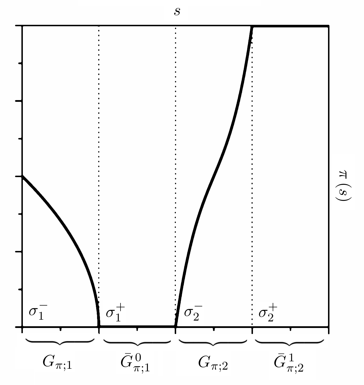
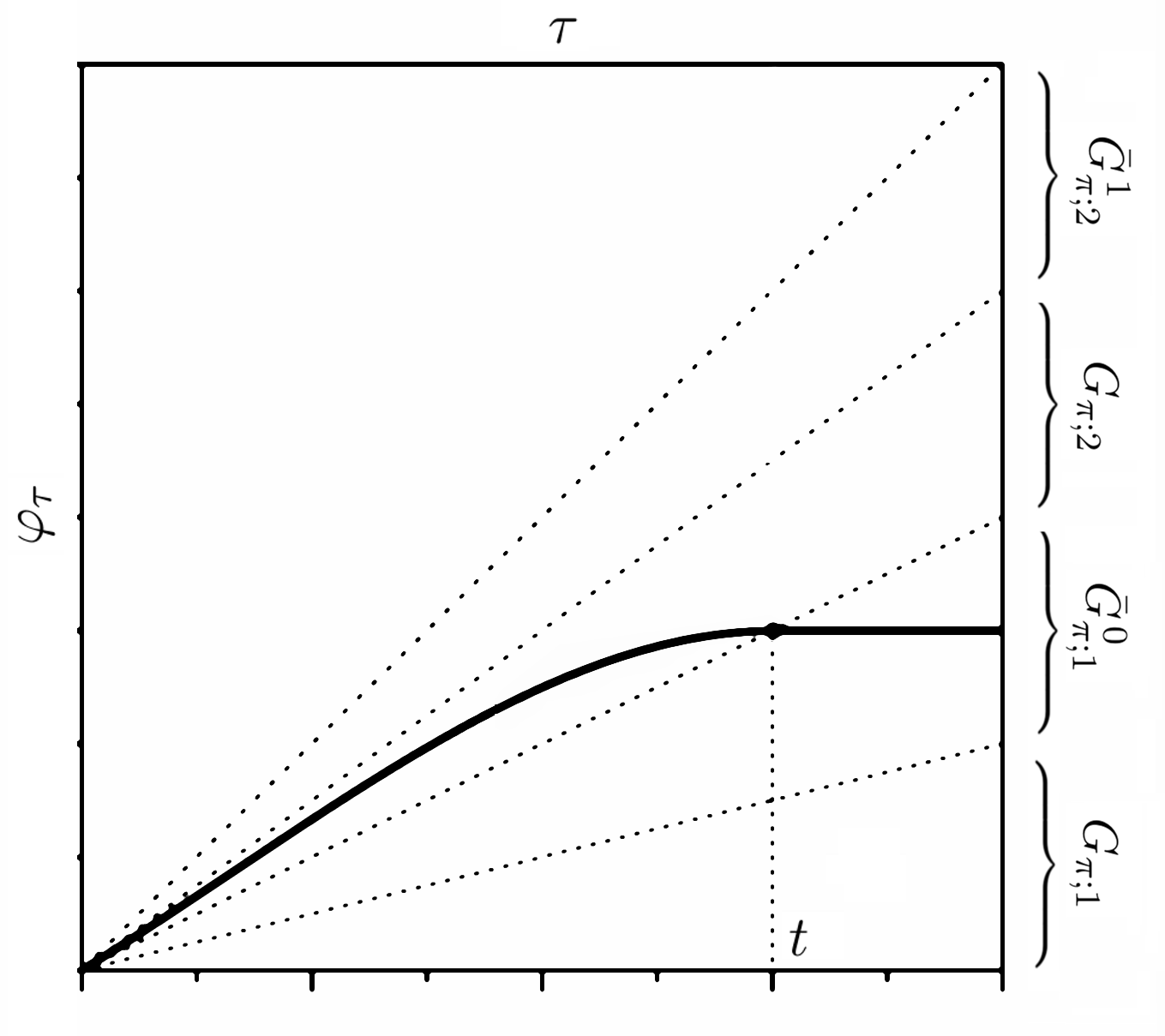
Figure 3.1. Example of urn function $\pi$ with relative $G_{\pi;i}$, $\bar{G}_{\pi;i}^{\alpha}$ intervals (upper figure) and trajectory with $\lim_{\tau\rightarrow 0}\tau^{-1}\varphi_{\tau}\in G_{\pi,2}$, $\varphi_{1}\in\bar{G}_{\pi;1}^{\,0}$, $S_{\pi}\left[\varphi\right]>-\infty$ (lower figure).

3.1.3. Extension to $\pi\in\left[0,1\right]$: surgery over $\mathcal{Q}$.

When we allow $\pi\left(s\right)$ to be eventually $0$ or $1$ quantities like $\left\|\pi\right\|^{-1}$, $\left\|\bar{\pi}\right\|^{-1}$, $\left\|\log\pi\right\|$, $\left\|\log\bar{\pi}\right\|$ may not be bounded and Lemmas 13 and 14 don’t hold anymore. Here we show that we can recover these two lemmas by a suitable surgery over the set $\mathcal{Q}$ to a priori exclude those trajectories for which $S_{\pi}\left[\varphi\right]=-\infty$.

Proof.

The key point is to notice that any $\varphi$ for which $\pi\left(\varphi_{\tau}/\tau\right)=0$ for $\tau\in\left[\tau_{1},\tau_{2}\right]$ with $\left|\tau_{1}-\tau_{2}\right|>0$ gives $S_{\pi}\left[\varphi\right]=-\infty$ unless $d\varphi_{\tau}=0$, or $d\varphi_{\tau}=1$ if $\pi\left(\varphi_{\tau}/\tau\right)=1$, in the same $\tau$ interval. To formally explain this we need some notation. Then, define

(3.18) $$G_{\pi}:=\left\{s\in\left[0,1\right]:\,\pi\left(s\right)\in\left(0,1\right)\right\},\,\partial G_{\pi}:=\mathrm{cl}\left(G_{\pi}\right)\setminus\mathrm{int}\left(G_{\pi}\right)$$

and organize the elements of $\partial G_{\pi}$ by increasing order by labeling them as follows:

(3.19) $$\partial G_{\pi}=:\left\{\sigma_{1}^{-},\sigma_{1}^{+},\sigma_{2}^{-},\sigma_{2}^{+},\,...\,,\,\sigma_{N}^{-},\sigma_{N}^{+}:\,\sigma_{i}^{-}<\sigma_{i}^{+},\sigma_{i}^{+}\leq\sigma_{i+1}^{-}\right\}$$

The above notation allows to define the sequence of intervals

(3.20) $$G_{\pi;i}:=\left(\sigma_{i}^{-},\sigma_{i}^{+}\right),\,1\leq i\leq N_{g},$$

such that $\pi\left(s\right)\in\left(0,1\right)$ for any $s\in G_{\pi;i}:=\left(\sigma_{i}^{-},\sigma_{i}^{+}\right)$ and $G_{\pi}:=\bigcup_{i}G_{\pi;i}$. We can also define the complementary sequence

(3.21) $$\bar{G}_{\pi;0}^{\,\alpha_{0}}:=\left[0,\sigma_{1}^{-}\right],\,\bar{G}_{\pi;i}^{\,\alpha_{i}}:=\left[\sigma_{i}^{+},\sigma_{i+1}^{-}\right],\,\bar{G}_{\pi;N_{g}}^{\,\alpha_{N_{g}}}:=\left[\sigma_{N}^{-},1\right]:\,\alpha_{i}\in\left\{0,1\right\},\,1\leq i\leq N_{g},$$

where $\alpha_{i}=\pi\left(s\right)$ for $s\in\left[\sigma_{i}^{+},\sigma_{i+1}^{-}\right]$, which is $0$ or $1$ by definition. By convention we take $\bar{G}_{\pi;0}^{\,\alpha_{0}}=\textrm{\O}$ if $\pi\left(0\right)\in\left(0,1\right)$ and $\bar{G}_{\pi;N_{g}}^{\,\alpha_{N_{g}}}=\textrm{\O}$ if $\pi\left(1\right)\in\left(0,1\right)$, and call by

(3.22) $$\alpha_{\pi}:=\left\{\alpha_{i}:\,0\leq i\leq N_{g}\right\}$$

the sequence of the $\alpha_{i}$. Clearly if $\alpha_{0}$ and $\alpha_{N_{g}}$ are not well defined we can exclude them from the above sequence and take $1\leq i\leq N_{g}-1$.

First we notice that every $\varphi$ such that $\tau^{-1}\varphi_{\tau}\in\bar{G}_{\pi;i}^{\,1}$, $d\varphi_{\tau}<1$ or $\tau^{-1}\varphi_{\tau}\in\bar{G}_{\pi;0}^{\,0}$, $d\varphi_{\tau}>0$ in some interval $\tau\in\left[\tau_{1},\tau_{2}\right]$ with $\left|\tau_{1}-\tau_{2}\right|>0$ gives $S_{\pi}\left[\varphi\right]=-\infty$. Then, we can discard all these cases and restrict our attention to the following subsets of $\mathcal{Q}$. The simplest subclasses of $\mathcal{Q}$ for which $S_{\pi}\left[\varphi\right]$ can be a bounded quantity are those where our $\varphi\in\mathcal{Q}$ is such that $\tau^{-1}\varphi_{\tau}\in G_{\pi;i}:=\left(\sigma_{i}^{-},\sigma_{i}^{+}\right)$

(3.23) $$\mathcal{Q}\left[G_{\pi;i}\right]:=\left\{\varphi\in\mathcal{Q}:\,\tau^{-1}\varphi_{\tau}\in G_{\pi;i}\right\}.$$

Anyway, we can build more functions that lives on contiguous intervals by taking $d\varphi_{\tau}=0$ when $\tau^{-1}\varphi_{\tau}\in\bar{G}_{\pi;i}^{\,0}$ or $d\varphi_{\tau}=d\tau$ when $\tau^{-1}\varphi_{\tau}\in\bar{G}_{\pi;i}^{\,1}$. As example, consider the subset of $\mathcal{Q}$ such that $\tau^{-1}\varphi_{\tau}\in\bar{G}_{\pi;i-1}^{\,0}\cup\,G_{\pi;i}$, $\lim_{\tau\rightarrow 0}\tau^{-1}\varphi_{\tau}\in G_{\pi,i}$ and $\varphi_{1}\in\bar{G}_{\pi;i-1}^{\,0}$: we can take $\varphi\in\mathcal{Q}$ such that $\sigma_{i}^{-}<\tau^{-1}\varphi_{\tau}<\sigma_{i}^{+}$ until some time $t\in\left(0,1\right)$, then $\varphi_{\tau}=\sigma_{i}^{+}$ for $t\leq\tau\leq 1$, with the obvious requirement that $t\geq\sigma_{i}^{+}/\sigma_{i-1}^{-}$ to ensure that $\varphi_{1}\in\bar{G}_{\pi;i-1}^{\,0}$ (see Figure 3.1). In the above trajectory the time interval $\left(t,1\right)$ in which $\log\pi\left(\tau^{-1}\varphi_{\tau}\right)=-\infty$ also have $d\varphi_{\tau}=0$, so that its contribution to the total value of $S_{\pi}$ is null.

(3.24) $$\int_{\tau\in\left[t,1\right]}\left[\,d\varphi_{\tau}\,\log\pi\left(\varphi_{\tau}/\tau\right)+d\tilde{\varphi}_{\tau}\,\log\bar{\pi}\left(\varphi_{\tau}/\tau\right)\right]=0.$$

The same can be done if $\alpha=1$ and $\tau^{-1}\varphi_{\tau}\in G_{\pi;i}\cup\,\bar{G}_{\pi;i}^{\,1}$ (ie, if $\lim_{\tau\rightarrow 0}\tau^{-1}\varphi_{\tau}\in G_{\pi,i}$ and $\varphi_{1}\in\bar{G}_{\pi;i}^{\,1}$): in this case we will chose $\sigma_{i}^{-}<\tau^{-1}\varphi_{\tau}<\sigma_{i}^{+}$ until some time $t\in\left[0,1\right]$, then $\varphi_{\tau}=\sigma_{i}^{+}t+\left(\tau-t\right)$ for $t\leq\tau\leq 1$ with $t\geq\left(1-\sigma_{i+1}^{-}\right)/\left(1-\sigma_{i}^{+}\right)$. In general, we can build functions that lives in arbitrary unions of contiguous intervals, as example $G_{\pi;i}\cup\,\bar{G}_{\pi;i}^{\,\alpha_{i}}\cup\,G_{\pi;i+1}\cup\,\bar{G}_{\pi;i+1}^{\,\alpha_{i+1}}\,...\,\cup\,\bar{G}_{\pi;j}^{\,\alpha_{j}}\cup\,G_{\pi;j+1}$, provided that $\alpha_{i}=\alpha_{i+1}=\,...\,=\alpha_{j}$. To give a general characterization of those functions define the following groups of intervals

(3.25) $$G_{\pi;i,j}^{\,0}:=\left\{G_{\pi;i},\,\bar{G}_{\pi;i}^{\,0},\,G_{\pi;i+1},\,\bar{G}_{\pi;i+1}^{\,0},\,...\,,\bar{G}_{\pi;j-1}^{\,0},\,G_{\pi;j}\right\},$$

(3.26) $$G_{\pi;i,j}^{\,1}:=\left\{G_{\pi;i},\,\bar{G}_{\pi;i}^{\,1},\,G_{\pi;i+1},\,\bar{G}_{\pi;i+1}^{\,1},\,...\,,\bar{G}_{\pi;j-1}^{\,1},\,G_{\pi;j}\right\},$$

(3.27) $$\bar{G}_{\pi;i,j}^{\,0}:=\left\{\bar{G}_{\pi;i-1}^{0},G_{\pi;i},\,\bar{G}_{\pi;i}^{\,0},\,G_{\pi;i+1},\,...\,,\bar{G}_{\pi;j-1}^{\,0},\,G_{\pi;j}\right\},$$

(3.28) $$\bar{G}_{\pi;i,j}^{\,1}:=\left\{G_{\pi;i},\,\bar{G}_{\pi;i}^{\,1},\,G_{\pi;i+1},\,.....\,,\bar{G}_{\pi;j-1}^{\,1},\,G_{\pi;j},\,\bar{G}_{\pi;j}^{1}\right\}.$$

From each of the above groups of intervals we can define a subset of $\mathcal{Q}$ as follows. First consider $G_{\pi;i,j}^{\,0}$, take some $s\in G_{\pi;i}$ and denote by $T_{i,j}$ a general time sequence

(3.29) $$T_{i,j}:=\left\{t_{k}\in\left[0,1\right]:\,i\leq k\leq j\right\}.$$

Then we can define a set of $T_{i,j}$ sequences

(3.30) $$T_{s}\left[G_{\pi;i,j}^{\,0}\right]:=\left\{T_{i+1,j}:\,0<\left(\sigma_{k}^{-}/\sigma_{k-1}^{+}\right)t{}_{k}\leq t_{k-1}\leq\left(s/\sigma_{i+1}^{-}\right)\right\}$$

and the associated set of trajectories $\mathcal{Q}_{s}[G_{\pi;i,j}^{\,0},\,T_{i+1,j}]\subseteq\mathcal{Q}$

(3.31) $$\mathcal{Q}_{s}\left[G_{\pi;i,j}^{\,0},\,T_{i+1,j}\right]:=\{\varphi\in\mathcal{Q}:\,i+1\leq k\leq j-1;\,\varphi_{1}=s;\\ \tau^{-1}\varphi_{\tau}\in G_{\pi;j},\,\tau\in\left[0,t_{j}\right];\,\varphi_{\tau}=\sigma_{k+1}^{-}t_{k+1},\,\tau\in\left[t_{k+1},t^{\prime}_{k+1}\right];\\ \tau^{-1}\varphi_{\tau}\in G_{\pi;k},\,\tau\in\left[t^{\prime}_{k+1},t_{k}\right];\,\varphi_{\tau}=\sigma_{k}^{-}t_{k},\,\tau\in\left[t_{k},t^{\prime}_{k}\right];\\ \tau^{-1}\varphi_{\tau}\in G_{\pi;i},\,\tau\in\left[t^{\prime}_{i+1},1\right];\,t_{k}^{{}^{\prime}}:=\left(\sigma_{k}^{-}/\sigma_{k-1}^{+}\right)t_{k}\},$$

with $\lim_{\tau\rightarrow 0}\tau^{-1}\varphi_{\tau}\in G_{\pi;j}$ and ending in $\varphi_{1}=s\in G_{\pi;j}$. At this point we can define

(3.32) $$\mathcal{Q}\left[G_{\pi;i,j}^{\,0}\right]:=\bigcup_{s\in G_{\pi;i}}\ \bigcup_{T_{i+1,j}\in\,T_{s}\left[G_{\pi;i,j}^{\,0}\right]}\ {\textstyle\mathcal{Q}_{s}\,[G_{\pi;i,j}^{\,0},\,T_{i+1,j}]},$$

which is the set of trajectories with $\lim_{\tau\rightarrow 0}\tau^{-1}\varphi_{\tau}\in G_{\pi;j}$ and $\varphi_{1}\in G_{\pi;i}$ for which $S_{\pi}\left[\varphi\right]$ may still be a bounded quantity. We can do the same for the remaining classes of sets. For $G_{\pi;i,j}^{\,1}$ we take $s\in G_{\pi;j}$, define

(3.33) $$T_{s}\left[G_{\pi;i,j}^{\,1}\right]:=\left\{T_{i,j-1}:\,0<\left(\bar{\sigma}_{k}^{-}/\bar{\sigma}_{k+1}^{+}\right)t{}_{k}\leq t_{k+1}\leq\left(\bar{s}/\bar{\sigma}_{i+1}^{-}\right)\right\},$$

(3.34) $$\mathcal{Q}_{s}\left[G_{\pi;i,j}^{\,1},\,T_{i,j-1}\right]:=\{\varphi\in\mathcal{Q}:\,i-1\leq k\leq j+1;\,\varphi_{1}=s;\\ \tau^{-1}\varphi_{\tau}\in G_{\pi;i},\,\tau\in\left[0,t_{i}\right];\,\varphi_{\tau}=\tau-\bar{\sigma}_{k-1}^{+}t_{k-1},\,\tau\in\left[t_{k-1},t^{\prime}_{k-1}\right];\\ \tau^{-1}\varphi_{\tau}\in G_{\pi;k},\,\tau\in\left[t^{\prime}_{k-1},t_{k}\right];\,\varphi_{\tau}=\tau-\bar{\sigma}_{k}^{+}t_{k},\,\tau\in\left[t_{k},t^{\prime}_{k}\right];\\ \tau^{-1}\varphi_{\tau}\in G_{\pi;j},\,\tau\in\left[t^{\prime}_{j-1},1\right];\,t_{k}^{{}^{\prime}}:=\left(\bar{\sigma}_{k}^{+}/\bar{\sigma}_{k+1}^{-}\right)t_{k}\},$$

to obtain set of trajectories with $\lim_{\tau\rightarrow 0}\tau^{-1}\varphi_{\tau}\in G_{\pi;i}$ and $\varphi_{1}\in G_{\pi;j}$

(3.35) $$\mathcal{Q}\left[G_{\pi;i,j}^{\,1}\right]:=\bigcup_{s\in G_{\pi;i}}\ \bigcup_{T_{i+1,j}\in\,T_{s}\left[G_{\pi;i,j}^{\,1}\right]}\ {\textstyle\mathcal{Q}_{s}\,[G_{\pi;i,j}^{\,1},\,T_{i,j-1}]}$$

associated to $G_{\pi;i,j}^{\,1}$. Then we take some $s\in\bar{G}_{\pi;i-1}^{\,0}$, define

(3.36) $$T_{s}\left[\bar{G}_{\pi;i,j}^{\,0}\right]:=\left\{T_{i,j}:\,0\leq t_{k}\leq\left(\sigma_{k}^{-}/\sigma_{k-1}^{+}\right)t{}_{k}\leq t_{k-1}<1;\,t_{i}=\left(s/\sigma_{i}^{-}\right)\right\},$$

(3.37) $$\mathcal{Q}_{s}\left[\bar{G}_{\pi;i,j}^{\,0},\,T_{i,j}\right]:=\{\varphi\in\mathcal{Q}:\,i+1\leq k\leq j;\,\tau^{-1}\varphi_{\tau}\in G_{\pi;j},\,\tau\in\left[0,t_{j}\right];\\ \varphi_{\tau}=\sigma_{k}^{-}t_{k},\,\tau\in\left[t_{k},t^{\prime}_{k}\right];\,\tau^{-1}\varphi_{\tau}\in G_{\pi;k-1},\,\tau\in\left[t^{\prime}_{k},t_{k-1}\right];\\ \varphi_{\tau}=st_{i},\,\tau\in\left[t_{i},1\right];\,t^{\prime}_{k}:=\left(\sigma_{k}^{-}/\sigma_{k-1}^{+}\right)t_{k}\}$$

and define trajectories with $\lim_{\tau\rightarrow 0}\tau^{-1}\varphi_{\tau}\in G_{\pi;j}$ and $\varphi_{1}\in\bar{G}_{\pi;i-1}^{\,0}$

(3.38) $$\mathcal{Q}\left[\bar{G}_{\pi;i,j}^{\,0}\right]:=\bigcup_{s\in\bar{G}_{\pi;i-1}}\ \bigcup_{T_{i,j}\in\,T_{s}\left[\bar{G}_{\pi;i,j}^{\,0}\right]}\ {\textstyle\mathcal{Q}_{s}\,[\bar{G}_{\pi;i,j}^{\,0},\,T_{i,j}]}.$$

Finally, let $s\in\bar{G}_{\pi;j}^{\,1}$,

(3.39) $$T_{s}\left[\bar{G}_{\pi;i,j}^{\,1}\right]:=\left\{T_{i,j}:\,0\leq t_{k}\leq\left(\bar{\sigma}_{k}^{-}/\bar{\sigma}_{k+1}^{+}\right)t{}_{k}\leq t_{k+1}<1;\,t_{j}=\left(\bar{s}/\bar{\sigma}_{i}^{-}\right)\right\},$$

(3.40) $$\mathcal{Q}_{s}\left[\bar{G}_{\pi;i,j}^{\,1},\,T_{i,j}\right]:=\{\varphi\in\mathcal{Q}:\,i\leq k\leq j-1;\,\tau^{-1}\varphi_{\tau}\in G_{\pi;i},\,\tau\in\left[0,t_{i}\right];\\ \varphi_{\tau}=\tau-\bar{\sigma}_{k}^{+}t_{k},\,\tau\in\left[t_{k},t^{\prime}_{k}\right];\,\tau^{-1}\varphi_{\tau}\in G_{\pi;k+1},\,\tau\in\left[t^{\prime}_{k},t_{k+1}\right];\\ \varphi_{\tau}=\tau-\bar{s},\,\tau\in\left[t_{j},1\right];\,t^{\prime}_{k}:=\left(\bar{\sigma}_{k}^{+}/\bar{\sigma}_{k+1}^{-}\right)t_{k}\},$$

and the set of trajectories with $\lim_{\tau\rightarrow 0}\tau^{-1}\varphi_{\tau}\in G_{\pi;i}$ and $\varphi_{1}\in\bar{G}_{\pi;j}^{\,1}$ be

(3.41) $$\mathcal{Q}\left[\bar{G}_{\pi;i,j}^{\,1}\right]:=\bigcup_{s\in\bar{G}_{\pi;j}}\ \bigcup_{T_{i,j}\in\,T_{s}\left[\bar{G}_{\pi;i,j}^{\,1}\right]}\ {\textstyle\mathcal{Q}_{s}\,[\bar{G}_{\pi;i,j}^{\,1},\,T_{i,j}]}.$$

By continuity of $\pi$ we observe that the number $N_{g}$ of connected intervals in which $\pi$ is $0$ or $1$ is finite, then also is the number of combination of contiguous intervals $G_{\pi;i,j}^{\,0}$, $G_{\pi;i,j}^{\,1}$, $\bar{G}_{\pi;i,j}^{\,0}$, and $\bar{G}_{\pi;i,j}^{\,1}$ satisfying the condition $\alpha_{i}=\alpha_{i+1}=\,...\,=\alpha_{j}=\alpha\in\left\{0,1\right\}$. Calling $N_{g}^{*}$ the number of these combination of intervals, plus the elementary intervals $G_{\pi;i}$, we can considerably lighten our notation by relabeling as $\mathcal{Q}_{k}$, $1\leq k\leq N_{g}^{*}$ their associated subsets of $\mathcal{Q}$ defined by Eq.s (3.32), (3.35), (3.38) and (3.41).

Since for any $\varphi$ that does not belong to $\mathcal{Q}_{k}$, $1\leq k\leq N_{g}^{*}$ we will find $S_{\pi}\left[\varphi\right]=-\infty$ we can use the relation $\mathbb{P}\left(\chi_{n}\in\mathcal{B}\right)=\sum_{i\leq k\leq N_{g}^{*}}\mathbb{P}\left(\chi_{n}\in\mathcal{B}\cap\mathcal{Q}_{k}\right)$ to conclude that

(3.42) $$\lim_{n\rightarrow\infty}n^{-1}\log\mathbb{P}\left(\chi_{n}\in\mathcal{B}\right)=\sup_{1\leq k\leq N^{*}}\lim_{n\rightarrow\infty}n^{-1}\log\mathbb{P}\left(\chi_{n}\in\mathcal{B}\cap\mathcal{Q}_{k}\right)$$

and restrict our attention to $\varphi\in\mathcal{Q}_{k}$. ∎

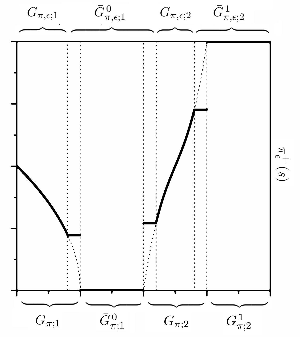
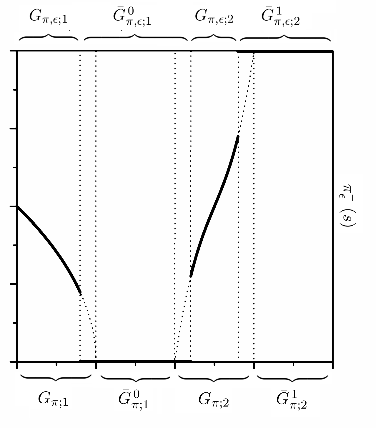
Figure 3.2. Functions $\pi_{\epsilon}^{+}$ (upper figure) and $\pi_{\epsilon}^{-}$ (lower figure) as defined by Eq.s (3.44) and (3.45) from the same urn function in Figure 3.1.

3.1.4. Extension to $\pi\in\left[0,1\right]$: singularities on the edges of $G_{\pi,i}$.

The above argument fixes the problem of having $\log\pi\left(\tau^{-1}\varphi_{\tau}\right)=-\infty$ when $\tau^{-1}\varphi_{\tau}\in\bar{G}_{\pi;i}^{\,0}$ (or $\log\bar{\pi}\left(\tau^{-1}\varphi_{\tau}\right)=-\infty$ when $\tau^{-1}\varphi_{\tau}\in\bar{G}_{\pi;i}^{\,1}$), but we still have $\pi\left(s\right)\rightarrow 0$ or $1$ when $s\rightarrow\sigma_{i}^{\pm}$, which prevent us from recovering Lemmas 13 and 14. To circumvent this last issue we can proceed as follows.

Proof.

Take some small $\epsilon>0$ and define $G_{\pi,\epsilon;i}$, $\bar{G}_{\pi,\epsilon;i}^{\,\alpha_{i}}$ as in Eq.s (3.25), (3.26), (3.27), (3.28) above with $\sigma_{i}^{-}+\epsilon$ in place of $\sigma_{i}^{-}$ and $\sigma_{i}^{+}-\epsilon$ in place of $\sigma_{i}^{+}$, such that some $\delta_{\epsilon}>0$ exists for which

(3.43) $$\sup_{i}\sup_{s\in G_{\pi,\epsilon;i}}\pi\left(s\right)\geq\delta_{\epsilon},\ \sup_{i}\sup_{s\in G_{\pi,\epsilon;i}}\bar{\pi}\left(s\right)\geq\delta_{\epsilon}.$$

Then, define the discontinuous functions $\pi_{\epsilon}^{+}\geq\pi$ and $\pi_{\epsilon}^{-}\leq\pi$ as follows:

(3.44) $$\pi_{\epsilon}^{+}:=\{\pi_{\epsilon}^{+}\left(s\right),\,s\in\left[0,1\right]:\,\pi_{\epsilon}^{+}\left(s\right)=\pi\left(s\right),\,s\in G_{\pi,\epsilon;i}:=\left(\sigma_{i}^{-}+\epsilon,\sigma_{i}^{+}-\epsilon\right);\\ \pi\left(s\right)=\pi\left(\sigma_{i}^{-}+\epsilon\right),\,s\in\left[\sigma_{i}^{-},\sigma_{i}^{-}+\epsilon\right];\,\pi_{\epsilon}^{+}\left(s\right)=\pi\left(\sigma_{i}^{+}-\epsilon\right),\,s\in\left[\sigma_{i}^{+}-\epsilon,\sigma_{i}^{+}\right]\},$$

(3.45) $$\pi_{\epsilon}^{-}:=\{\pi_{\epsilon}^{-}\left(s\right),\,s\in\left[0,1\right]:\,\pi_{\epsilon}^{-}\left(s\right)=\pi\left(s\right),\,s\in G_{\pi,\epsilon;i}:=\left(\sigma_{i}^{-}+\epsilon,\sigma_{i}^{+}-\epsilon\right);\\ \pi_{\epsilon}^{-}\left(s\right)=\alpha_{\,i-1},\,s\in\left[\sigma_{i}^{-},\sigma_{i}^{-}+\epsilon\right];\,\pi_{\epsilon}^{-}\left(s\right)=\alpha_{i},\,s\in\left[\sigma_{i}^{+}-\epsilon,\sigma_{i}^{+}\right]\}.$$

Our proof will consist in showing Theorem 1 for the above modified urn functions and then provide an argument to take $\epsilon\rightarrow 0$.

Let first consider $\pi_{\epsilon}^{+}$. Since by definition we can bound $\pi_{\epsilon}^{+}\left(s\right)\geq\delta_{\epsilon}$ and $\bar{\pi}_{\epsilon}^{+}\left(s\right)\geq\delta_{\epsilon}$ when $s\in G_{\pi;i}$, it is clear that both Lemmas 13, 14 would hold again for $\pi_{\epsilon}^{+}$ in each metric space $(\mathcal{Q}_{k},\,\left\|\cdot\right\|)$, with some $W_{\pi_{\epsilon}^{+}}\left(s,\,\epsilon\right)$ such that $\lim_{s\rightarrow 0,}W_{\pi_{\epsilon}^{+}}\left(s,\,\epsilon\right)=0$ for any $\epsilon>0$ in place of of $W_{\pi}\left(s\right)$. Then we can apply the proof for $\pi\in\left(0,1\right)$ to the events $\mathcal{B}\cap\mathcal{Q}_{k}$, obtaining for $\pi_{\epsilon}^{+}$

(3.46) $$\limsup_{n\rightarrow\infty}n^{-1}\log\mathbb{P}\left(\chi_{n}\in\mathcal{B}\right)\leq-\inf_{1\leq k\leq N^{*}}\inf_{\varphi\in\mathcal{\mathrm{cl}}\left(\mathcal{B\,}\cap\mathcal{Q}_{k}\right)}I_{\pi_{\epsilon}}\left[\varphi\right]=-\inf_{\varphi\in\mathcal{\mathrm{cl}\left(\mathcal{B}\right)}}I_{\pi_{\epsilon}^{+}}\left[\varphi\right],$$

(3.47) $$\liminf_{n\rightarrow\infty}n^{-1}\log\mathbb{P}\left(\chi_{n}\in\mathcal{B}\right)\geq-\inf_{1\leq k\leq N^{*}}\inf_{\varphi\in\mathcal{\mathrm{int}}\left(\mathcal{B\,}\cap\mathcal{Q}_{k}\right)}I_{\pi_{\epsilon}^{+}}\left[\varphi\right]=-\inf_{\varphi\in\mathcal{\mathrm{int}\left(\mathcal{B}\right)}}I_{\pi_{\epsilon}^{+}}\left[\varphi\right].$$

We can produce an identical reasoning for $\pi_{\epsilon}^{-}$, provided we consider $G_{\pi,\epsilon;i}$ on place of of $G_{\pi;i}$ in the definitions of the sets $\mathcal{Q}_{k}$, $1\leq k\leq N_{g}^{*}$: we will relabel them as $\mathcal{Q}_{\epsilon;k}$, $1\leq k\leq N_{g}^{*}$ to emphasize the dependence on $\epsilon$ of the intervals. Then, also for $\pi_{\epsilon}^{-}$ we can write

(3.48) $$\limsup_{n\rightarrow\infty}n^{-1}\log\mathbb{P}\left(\chi_{n}\in\mathcal{B}\right)\leq-\inf_{1\leq k\leq N^{*}}\inf_{\varphi\,\in\mathcal{\mathrm{cl}}\left(\mathcal{B}\,\cap\,\mathcal{Q}_{\epsilon;k}\right)}I_{\pi_{\epsilon}^{-}}\left[\varphi\right]=-\inf_{\varphi\,\in\mathcal{\mathrm{cl}\left(\mathcal{B}\right)}}I_{\pi_{\epsilon}^{-}}\left[\varphi\right],$$

(3.49) $$\liminf_{n\rightarrow\infty}n^{-1}\log\mathbb{P}\left(\chi_{n}\in\mathcal{B}\right)\geq-\inf_{1\leq k\leq N^{*}}\inf_{\varphi\,\in\mathcal{\mathrm{cl}}\left(\mathcal{B}\,\cap\,\mathcal{Q}_{\epsilon;k}\right)}I_{\pi_{\epsilon}^{-}}\left[\varphi\right]=-\inf_{\varphi\in\,\mathcal{\mathrm{int}\left(\mathcal{B}\right)}}I_{\pi_{\epsilon}^{-}}\left[\varphi\right].$$

The last step is to prove that for any Borel subset $\mathcal{B}$ of $\mathcal{Q}$

(3.50) $$\lim_{\epsilon\rightarrow 0}\,\inf_{\varphi\,\in\,\mathcal{B\,}\cap\,\mathcal{Q}_{k}}\,I_{\pi_{\epsilon}^{+}}\left[\varphi\right]=\lim_{\epsilon\rightarrow 0}\,\inf_{\varphi\,\in\,\mathcal{B\,}\cap\,\mathcal{Q}_{\epsilon;k}}\,I_{\pi_{\epsilon}^{-}}\left[\varphi\right]=\inf_{\varphi\,\in\,\mathcal{B\,}\cap\,\mathcal{Q}_{k}}\,I_{\pi}\left[\varphi\right].$$

We will explicitly prove this relation only for subsets of the kind $\mathcal{Q\,}[\,G_{\pi;i,j}^{\,0}]$, since all other cases can be shown using the same technique with minimal modifications. Then let $\mathcal{Q\,}[\,G_{\pi;i,j}^{\,0}]$ as in Eq. (3.32) and call $\mathcal{Q\,}[\,G_{\pi,\epsilon;i,j}^{\,0}]$ its version with $\sigma_{k}^{+}-\epsilon$ on place of of $\sigma_{k}^{+}$ and $\sigma_{k}^{-}+\epsilon$ on place of of $\sigma_{k}^{-}$. By Eq. (3.32), to prove Eq. (3.50) it suffices to show that

(3.51) $$\lim_{\epsilon\rightarrow 0}\ \inf_{\varphi\,\in\,\mathcal{B\,}\cap\,\mathcal{Q}_{s}[G_{\pi;i,j}^{\,0},\,T_{i+1,j}]}\,I_{\pi_{\epsilon}^{+}}\left[\varphi\right]=\lim_{\epsilon\rightarrow 0}\ \inf_{\varphi\,\in\,\mathcal{B\,}\cap\mathcal{Q}_{s}[G_{\pi,\epsilon;i,j}^{\,0},\,T_{\epsilon,i+1,j}^{*}]}\,I_{\pi_{\epsilon}^{-}}\left[\varphi\right]=\inf_{\varphi\,\in\,\mathcal{B\,}\cap\,\mathcal{Q}_{s}[G_{\pi;i,j}^{\,0},\,T_{i+1,j}]}\,I_{\pi}\left[\varphi\right],$$

with $s\in G_{\pi;i}$, $T_{i+1,j}\in T_{s}[G_{\pi;i,j}^{\,0}]$ and

(3.52) $$T_{\epsilon,i+1,j}^{*}:=\left\{t_{\epsilon,k}:=\left(\sigma_{k}^{-}/\left(\sigma_{k}^{-}+\epsilon\right)\right)t_{k}:\,i+1\leq k\leq j\right\}.$$

Then, define the optimal trajectories of the variational problems for $\pi_{\epsilon}^{+}$ and $\pi_{\epsilon}^{-}$:

(3.53) $$\varphi^{+}:\,I_{\pi_{\epsilon}^{+}}[\varphi^{+}]=\,\,\inf_{\varphi\,\in\,\mathcal{B\,}\cap\,\mathcal{Q}_{s}[G_{\pi;i,j}^{\,0},\,T_{i+1,j}]}\,\,I_{\pi_{\epsilon}^{+}}\left[\varphi\right],$$

(3.54) $$\varphi^{-}:\,I_{\pi_{\epsilon}^{-}}[\varphi^{-}]=\inf_{\varphi\,\in\,\mathcal{B\,}\cap\mathcal{Q}_{s}[G_{\pi,\epsilon;i,j}^{\,0},\,T_{\epsilon,i+1,j}^{*}]}I_{\pi_{\epsilon}^{-}}\left[\varphi\right].$$

Since $\varphi^{+}$ may not belong to $\mathcal{Q}_{s}[G_{\pi,\epsilon;i,j}^{\,0},\,T_{\epsilon,i+1,j}^{*}]$ it will be useful to introduce a modified trajectory $\varphi_{\epsilon}^{+}:=\left\{\varphi_{\epsilon;\tau}^{+}:\,\tau\in\left[0,1\right]\right\}$, defined as follows

(3.55) $$\varphi_{\epsilon;\tau}^{+}:=\left\{\begin{array}[]{l}\underset{\,}{\sigma_{k}^{+}t^{\prime}_{k+1},}\\ \inf\left\{\left(\sigma_{k}^{-}+\epsilon\right)\tau,\,\sup\left\{\varphi_{\tau}^{+},\left(\sigma_{k}^{+}-\epsilon\right)\tau\right\}\right\},\\ \overset{\,}{\sigma_{k}^{-}t_{k},}\end{array}\ \begin{array}[]{l}\underset{\,}{t^{\prime}_{k+1}<\tau<t^{\prime}_{\epsilon,k+1},}\\ \underset{\,}{t^{\prime}_{\epsilon,k+1}\leq\tau<t{}_{\epsilon,k},}\\ t{}_{\epsilon,k}<\tau<t{}_{k},\end{array}\right.$$

with $i\leq k\leq j$ and $t^{\prime}_{\epsilon,k}=\left(\left(\sigma_{k}^{-}+\epsilon\right)/\left(\sigma_{k-1}^{+}-\epsilon\right)\right)t_{\epsilon,k}$ as for $t^{\prime}_{k}$. The scope of this modified trajectory will be clear after we state the following auxiliary relations. By definition of $\varphi_{\tau}^{-}$ as optimal trajectory for $I_{\pi_{\epsilon}^{-}}$ we find $I_{\pi_{\epsilon}^{-}}[\varphi_{\epsilon}^{+}]\geq I_{\pi_{\epsilon}^{-}}[\varphi^{-}]$, while by definition of $\varphi_{\tau}^{+}$ we have $I_{\pi_{\epsilon}^{+}}[\varphi^{-}]\geq I_{\pi_{\epsilon}^{+}}[\varphi^{+}]$. Now let $\Gamma_{\epsilon}:=I_{\pi_{\epsilon}^{+}}[\varphi^{+}]-I_{\pi_{\epsilon}^{+}}[\varphi_{\epsilon}^{+}]$. By continuity of $I_{\pi_{\epsilon}^{+}}$ we can write

(3.56) $$\lim_{\epsilon\rightarrow 0}\Gamma_{\epsilon}:=\lim_{\epsilon\rightarrow 0}\,(\,I_{\pi_{\epsilon}^{+}}[\varphi^{+}]-I_{\pi_{\epsilon}^{+}}[\varphi_{\epsilon}^{+}]\,)=0.$$

Then, consider $I_{\pi_{\epsilon}^{+}}[\varphi_{\epsilon}^{+}]$ and $I_{\pi_{\epsilon}^{-}}[\varphi_{\epsilon}^{+}]$. Since $\pi_{\epsilon}^{+}\left(\tau^{-1}\varphi_{\epsilon;\tau}^{+}\right)=\pi_{\epsilon}^{-}\left(\tau^{-1}\varphi_{\epsilon;\tau}^{+}\right)$ for $\tau\in[t^{\prime}_{\epsilon,k+1},t{}_{\epsilon,k},]$ by construction their difference lies only in the intervals when $(t^{\prime}_{k},\,t^{\prime}_{\epsilon,k})$ and $\left(t{}_{\epsilon,k},\,t{}_{k}\right)$, so that we can bound as

(3.57) $$\left|\Delta_{\epsilon}\right|:=|I_{\pi_{\epsilon}^{+}}[\varphi_{\epsilon}^{+}]-I_{\pi_{\epsilon}^{-}}[\varphi_{\epsilon}^{+}]|=\sum_{i\leq k\leq j}\int_{\tau\in(t^{\prime}_{k+1},\,t^{\prime}_{\epsilon,k+1})\cup(t{}_{\epsilon,k},\,t{}_{k})}d\tau\,\left|\log\bar{\pi}_{\epsilon}^{+}\left(\tau^{-1}\varphi_{\tau}\right)\right|=\\ =\left(j-i\right)\left[\left(t^{\prime}_{k+1}-t^{\prime}_{\epsilon,k+1}\right)+\left(t{}_{\epsilon,k}-t{}_{k}\right)\right]\left|\log\bar{\pi}_{\epsilon}^{+}\left(t_{\epsilon}^{-1}\left(\sigma_{k}^{+}-\epsilon\right)\right)\right|\leq\\ \leq\left(j-i\right)\left(\left|t^{\prime}_{k+1}-t^{\prime}_{\epsilon,k+1}\right|+\left|t{}_{k+1}-t{}_{\epsilon,k+1}\right|\right)\delta_{\epsilon}.$$

The same considerations hold for $I_{\pi_{\epsilon}^{+}}[\varphi_{\epsilon}^{-}]$ and $I_{\pi_{\epsilon}^{-}}[\varphi_{\epsilon}^{-}]$, for which again one finds $I_{\pi_{\epsilon}^{+}}[\varphi^{-}]-I_{\pi_{\epsilon}^{-}}[\varphi^{-}]=\Delta_{\epsilon}.$ Collecting the above relations we find

(3.58) $$I_{\pi_{\epsilon}^{-}}[\varphi^{-}]\leq I_{\pi_{\epsilon}^{-}}[\varphi_{\epsilon}^{+}]=I_{\pi_{\epsilon}^{+}}[\varphi_{\epsilon}^{+}]+\Delta_{\epsilon}=I_{\pi_{\epsilon}^{+}}[\varphi^{+}]-\Gamma_{\epsilon}+\Delta_{\epsilon},$$

(3.59) $$I_{\pi_{\epsilon}^{+}}[\varphi^{+}]\leq I_{\pi_{\epsilon}^{+}}[\varphi^{-}]=I_{\pi_{\epsilon}^{-}}[\varphi^{-}]+\Delta_{\epsilon},$$

from which follows that

(3.60) $$\lim_{\epsilon\rightarrow 0}I_{\pi_{\epsilon}^{+}}[\varphi^{+}]=\lim_{\epsilon\rightarrow 0}I_{\pi_{\epsilon}^{-}}[\varphi^{-}].$$

Now consider the optimal trajectory $\varphi^{*}$ of the variational problem for the original $\pi$

(3.61) $$\varphi^{*}:\,I_{\pi}[\varphi^{*}]=\inf_{\varphi\,\in\,\mathcal{B}\,\cap\,\mathcal{Q}_{s}\,[\,G_{\pi;i,j}^{\,0},\,T_{i+1,j}]}I_{\pi}\left[\varphi\right].$$

By the above definition we have $I_{\pi}\left[\varphi^{*}\right]\leq I_{\pi}\left[\varphi^{-}\right]$ and since $\pi^{-}\left(\tau^{-1}\varphi_{\tau}^{-}\right)=\pi\left(\tau^{-1}\varphi_{\tau}^{-}\right)$ for $\tau\in[t^{\prime}_{\epsilon,k+1},t{}_{\epsilon,k}]$ we can bound the difference between $I_{\pi_{\epsilon}^{-}}\left[\varphi^{-}\right]$ and $I_{\pi}\left[\varphi^{-}\right]$ as

(3.62) $$\left|\Delta^{\prime}_{\epsilon}\right|:=|I_{\pi}\left[\varphi^{-}\right]-I_{\pi_{\epsilon}^{-}}\left[\varphi^{-}\right]|=\sum_{i\leq k\leq j}\int_{\tau\in(t^{\prime}_{k+1},\,t^{\prime}_{\epsilon,k+1})\cup(t{}_{\epsilon,k},\,t{}_{k})}d\tau\,\left|\log\bar{\pi}\left(\tau^{-1}\varphi_{\tau}\right)\right|\leq\\ \leq\left(j-i\right)\left(\left|t^{\prime}_{k+1}-t^{\prime}_{\epsilon,k+1}\right|+\left|t{}_{k+1}-t{}_{\epsilon,k+1}\right|\right)\delta_{\epsilon}.$$

As $\pi\leq\pi_{\epsilon}^{+}$ by construction we can also conclude that $I_{\pi_{\epsilon}^{+}}\left[\varphi^{*}\right]\leq I_{\pi}\left[\varphi^{*}\right]$, while by definition of $\varphi^{+}$ as optimal trajectory for $I_{\pi_{\epsilon}^{+}}$ we can write $I_{\pi_{\epsilon}^{+}}\left[\varphi^{+}\right]\leq I_{\pi_{\epsilon}^{+}}\left[\varphi^{*}\right]$. Collecting all those relations we obtain the following inequalities

(3.63) $$I_{\pi_{\epsilon}^{+}}\left[\varphi^{+}\right]\leq I_{\pi}\left[\varphi^{*}\right]\leq I_{\pi_{\epsilon}^{-}}\left[\varphi^{-}\right]-\Delta^{\prime}_{\epsilon},$$

and by taking $\epsilon\rightarrow 0$ we can finally write that

(3.64) $$\lim_{\epsilon\rightarrow 0}I_{\pi_{\epsilon}^{+}}[\varphi^{+}]\leq I_{\pi}\left[\varphi^{*}\right]\leq\lim_{\epsilon\rightarrow 0}I_{\pi_{\epsilon}^{-}}[\varphi^{-}],$$

which, together with Eq. (3.60), proves Eq. (3.51). This completes our extension of Theorem 1 to the whole set of urn function $\mathcal{U}$ in case we take as initial condition $X_{n,1}$ uniformly distributed on $\left[0,1\right]$. ∎

3.1.5. Initial conditions and time-inhomogeneous functions.

First we deal with the influence of initial conditions on the large deviation properties of our urn process. Until now we considered processes with initial condition $X_{n,1}$ uniformly distributed on $\left[0,1\right]$, the following lemma shows that fixing $X_{n,m}$ for some $m>0$ will not affect the rate function if $\pi\in\left(0,1\right)$, provided that $m$ is finite and $0\leq X_{n,m}\leq m$.

Lemma 16.

Let $X_{n}$ be a urn process with urn function $\pi\in\left(0,1\right)$ and initial conditions $0<X_{n,m}<m<\infty$. Then, the rate function is independent from these initial conditions.

Proof.

Let $\varphi\in\mathcal{Q}_{n}$, $x_{m,n}=m^{-1}X_{m,n}$ and $\epsilon_{n,\tau}$ as in Lemma 14. If $\pi\in\left(0,1\right)$ then $\left\|\log\pi\right\|$ and $\left\|\log\bar{\pi}\right\|$ are bounded quantities and we can use the estimates of Lemma 14 to obtain

(3.65) $$n^{-1}\left|\log\mathbb{P}\left(\chi_{n}=\varphi\,|\,\varphi_{m/n}=\left(m/n\right)x_{m,n}\right)-\log\mathbb{P}\left(\chi_{n}=\varphi\right)\right|\leq\\ \leq\int_{\tau\in\left[0,m/n\right]}d\varphi_{\tau}\,\left|\log\pi\left({\textstyle\left(\varphi_{\tau}+\epsilon_{n,\tau}\right)/\tau}\right)\right|+\int_{\tau\in\left[0,m/n\right]}d\tilde{\varphi}_{\tau}\,\left|\log\bar{\pi}\left(\left(\varphi_{\tau}+\epsilon_{n,\tau}\right)/\tau\right)\right|\leq\\ \leq\left(\left\|\log\pi\right\|+\left\|\log\bar{\pi}\right\|\right)m/n.$$

This difference vanishes as $n\rightarrow\infty$ for any $\varphi\in\mathcal{Q}_{n}$. This obviously implies that the LDPs governing the two processes share the same rate function. ∎

Now consider $\pi\in\left[0,1\right]$. By applying the steps to extend the proof of Theorem 1 we can easily convince that the only influence on LDPs arising from fixing $\varphi_{m/n}=\left(m/n\right)x_{m,n}$ comes from the fact that some trajectories could be forbidden, since by continuity of $\varphi_{\tau}$ a trajectory from $\varphi_{m/n}=\left(m/n\right)x_{m,n}$ to $\varphi_{1}=s$ may have to cross intervals where $\pi\left(\tau^{-1}\varphi_{\tau}\right)$ is $0$ or $1$ without having at the same time $d\varphi_{\tau}=0$ or $1$, which is a necessary condition to ensure that $S_{\pi}\left[\varphi\right]>-\infty$.

As example, consider an urn function such that $\pi\left(s\right)=0$ for some $s\in\left[\sigma_{1}^{+},\sigma_{2}^{-}\right]$, $0<\sigma_{1}^{+}<\sigma_{2}^{-}<1$, and $\pi\left(s\right)>0$ otherwise. As before, we can define the intervals $G_{\pi;1}:=\left[0,\sigma_{1}^{+}\right)$, $\bar{G}_{\pi;1}^{\,0}:=\left[\sigma_{1}^{+},\sigma_{2}^{-}\right]$ and $G_{\pi;2}:=\left(\sigma_{2}^{-},1\right]$. Then, take $\left(m/n\right)^{-1}\varphi_{m/n}=x_{m,n}\in G_{\pi;1}$ for some $m<\infty$. Since any trajectory $\varphi$ that reach $G_{\pi;2}$ from $G_{\pi;1}$ would require that $\tau^{-1}\varphi_{\tau}$ crosses $\bar{G}_{\pi;1}^{\,0}$ with some $d\varphi>0$, we conclude that such trajectory will return $S_{\pi}\left[\varphi\right]=-\infty$. Hence any allowed trajectory with $\left(m/n\right)^{-1}\varphi_{m/n}=x_{m,n}\in G_{\pi;1}$ would be confined in $G_{\pi;1}$, like a process with same initial condition and a modified urn function $\pi^{*}\left(s\right)=\pi\left(s\right)$ for $s\in G_{\pi;1}$ and $\pi^{*}\left(s\right)=0$ otherwise.

In general, the allowed interval $\left[z_{-}^{*},z_{+}^{*}\right]$ of $\tau^{-1}\varphi_{\tau}$ for trajectories with $\left(m/n\right)^{-1}\varphi_{m/n}=x_{n,m}$ will run from the highest non isolated value of $s$ reachable from $x_{n,m}$ and such that $\pi\left(s\right)=1$ to the lowest reachable non isolated $s$ such that $\pi\left(s\right)=0$, since those points acts as uncrossable walls for $\tau^{-1}\varphi_{\tau}$, while all other values contained in $\left[z_{-}^{*},z_{+}^{*}\right]$ can be crossed at least by trajectories of the type presented in the proof of Theorem 1 above.

Notice that in the above informal definition we specified that the point must be non isolated, since isolated points may be eventually crossed due to the discontinuous nature of the process at finite $n$. To avoid this inconsistencies we define $Z_{\pi,x_{m,n}}^{*}$ as the $\limsup$ of the subsets of $\left[0,1\right]$ that the process $k^{-1}X_{n,k}$ is allowed to hit at time $k=n$ with positive probability when we take $\mathbb{P}(x_{n,m}=m^{-1}X_{m})=1$ for some $m\leq n$, $0\leq X_{m}\leq m$ and $n<\infty$.

(3.66) $$Z_{\pi,x_{m,n}}^{*}:=\limsup_{n\rightarrow\infty}\left\{Z:\,\mathbb{P}\left(x_{n,n}\in Z\,|\,x_{n,m}=m^{-1}X_{m}\right)=1\right\}.$$

The above set is obviously an interval since, as said before, any internal point can be reached by trajectories of the type described in the proof of Theorem 1. Hence, we can say that $Z_{\pi,x_{m,n}}^{*}:=\left[z_{-}^{*},z_{+}^{*}\right]$, with $z_{-}^{*}$ and $z_{+}^{*}$ defined as in the statement of Corollary 2.

That said, it is clear that computing a LDP for a process with initial condition $x_{n,m}$ would be like computing it with initial condition $X_{n,1}$ uniformly distributed on $\left[0,1\right]$ once we have discarded from $\pi$ the forbidden zones. This can be done by considering a modified $\pi^{*}$ with $\pi^{*}\left(s\right)=1$ in the forbidden interval $s\in\left[0,z_{-}^{*}\right)$ on the left of $Z_{\pi,x_{m,n}}^{*}$ and $\pi^{*}\left(s\right)=0$ in $s\in\left(z_{+}^{*},1\right]$ on the right of $Z_{\pi,x_{m,n}}^{*}$,

(3.67) $$\pi^{*}\left(s\right):=\mathbb{I}_{\{s\in\left[0,z_{-}^{*}\right)\}}+\pi\left(s\right)\mathbb{I}_{\{s\in\left[z_{-}^{*},z_{+}^{*}\right]\}},$$

so that the probability mass initially distributed on $\left[0,1\right]$ gets pushed inside $Z_{\pi,x_{m,n}}^{*}$ in finite time, simulating the initial condition at least for what concerns the LDPs computation.

It remains to prove Corollary 3 about time-inhomogeneous functions. In this case we considered only the subclass $\pi\in\left(0,1\right)$, for which the proof is straightforward

Proof.

Let $\pi\in\mathcal{U}$ with $0<\pi<1$ and let $\pi_{n}\in\mathcal{U}$, $\pi_{n}\in\left(0,1\right)$ such that $\left|\pi_{n}\left(s\right)-\pi\left(s\right)\right|\leq\delta_{n}$, $\lim_{n}\delta_{n}=0$ for all $s\in\left[0,1\right]$. By lemma 14 it suffices to show that $\left|S_{\pi_{n}}\left[\varphi\right]-S_{\pi}\left[\varphi\right]\right|\rightarrow 0$ as $n\rightarrow 0$. We can bound $\left|S_{\pi_{n}}\left[\varphi\right]-S_{\pi}\left[\varphi\right]\right|$ as follows

$$\left|S_{\pi_{n}}\left[\varphi\right]-S_{\pi}\left[\varphi\right]\right|\leq\int_{\tau\in\left[0,1\right]}d\varphi_{\tau}\,\left|\log\pi_{n}\left(\varphi_{\tau}/\tau\right)-\log\pi\left(\varphi_{\tau}/\tau\right)\right|+\\ +\int_{\tau\in\left[0,1\right]}d\tilde{\varphi}_{\tau}\,\left|\log\bar{\pi}_{n}\left(\varphi_{\tau}/\tau\right)-\log\bar{\pi}\left(\varphi_{\tau}/\tau\right)\right|\leq\\ \leq\int_{\tau\in\left[0,1\right]}d\varphi_{\tau}\,\delta_{n}/\left|\pi\left(\varphi_{\tau}/\tau\right)\right|+\int_{\tau\in\left[0,1\right]}d\tilde{\varphi}_{\tau}\,\delta_{n}/\left|\bar{\pi}\left(\varphi_{\tau}/\tau\right)\right|\leq\\ \leq\left[1/\left(1-\left\|\bar{\pi}\right\|\right)+1/\left(1-\left\|\pi\right\|\right)\right]\delta_{n}.$$

Since for $0<\pi<1$ we have $\left\|\bar{\pi}\right\|<\infty$, $\left\|\pi\right\|<\infty$, the above bound vanishes as $\delta_{n}\rightarrow 0$ and the proof is completed. ∎

3.2. Entropy of the event $X_{n,n}=\left\lfloor sn\right\rfloor$.

In this section we use the variational representation of Sample-Path LDPs to show Theorem 4 and Corollaries 5, 6, 7. Since the event $\left\{X_{n,n}=\left\lfloor sn\right\rfloor\right\}$ is slightly finer than those usually considered in large deviations theory, its analysis requires some additional estimates. Moreover, note that $\mathcal{Q}_{s}$ is not an $I_{\pi}-$continuity set because of the fixed endpoint condition $\varphi_{1}=s$, which implies $\mathrm{cl}\left(\mathcal{Q}_{s}\right)=\varnothing$. We circumvent this problem as follows

Lemma 17.

Let $s\in\left[0,1\right]$, $\delta>0$ and define $\mathcal{Q}_{s,\delta}:={\textstyle\bigcup_{\,u-s\in\left[0,\delta\right]}}\,\mathcal{Q}_{u},$ where $\mathcal{Q}_{s}:=\left\{\varphi\in\mathcal{Q}:\,\varphi_{1}=s\right\}$, then

(3.68) $$\lim_{n\rightarrow\infty}n^{-1}\log\mathbb{P}\left(\left\lfloor sn\right\rfloor\leq X_{n,n}\leq\left\lfloor\left(s+\delta\right)n\right\rfloor\right)=-\inf_{\varphi\in\mathcal{Q}_{s,\delta}}I_{\pi}\left[\varphi\right].$$

Proof.

Since $\mathcal{Q}_{s,\delta}:={\textstyle\bigcup_{\,u-s\in\left[0,\delta\right]}}\,\mathcal{Q}_{u}$ is an $I_{\pi}-$continuity set when $s\in\left[0,1\right]$ and $\delta>0$, by Theorem 1 we have

(3.69) $$\lim_{n\rightarrow\infty}n^{-1}\log\mathbb{P}\left(\chi_{n}\in\mathcal{Q}_{s,\delta}\right)=-\inf_{\varphi\in\mathcal{Q}_{s,\delta}}I_{\pi}\left[\varphi\right].$$

Then, let $0<\nu<\delta$ so that we can write

(3.70) $$-\inf_{\varphi\in\mathcal{Q}_{s,\delta-\nu}}I_{\pi}\left[\varphi\right]=\lim_{n\rightarrow\infty}n^{-1}\log\mathbb{P}\left(\chi_{n}\in\mathcal{Q}_{s,\delta-\nu}\right)\leq\\ \leq\lim_{n\rightarrow\infty}n^{-1}\log\mathbb{P}\left(\left\lfloor sn\right\rfloor\leq X_{n,n}\leq\left\lfloor\left(s+\delta\right)n\right\rfloor\right)\leq\\ \leq\lim_{n\rightarrow\infty}n^{-1}\log\mathbb{P}\left(\chi_{n}\in\mathcal{Q}_{s,\delta+\nu}\right)=-\inf_{\varphi\in\mathcal{Q}_{s,\delta+\nu}}I_{\pi}\left[\varphi\right].$$

Since $I_{\pi}$ is continuous on $\left(\mathcal{Q},\left\|\cdot\right\|\right)$ and $\mathcal{Q}_{s,\delta^{\prime}}\subset\mathcal{Q}_{s,\delta}\subset\mathcal{Q}$ for every $\delta^{\prime}<\delta$, we can take the limit $\nu\rightarrow 0$ and the proof is completed. ∎

3.2.1. Proof of Theorem 4.

Before starting, we remind some notation. Let $\varphi:=\left\{\varphi_{\tau}:\tau\in\left[0,1\right]\right\}$ and let $Y_{n,k}\left(\varphi\right):=n\varphi_{k}$, $\delta Y_{n,k}\left(\varphi\right):=n\left(\varphi_{k+1}-\varphi_{k}\right)$ as in Eq. (3.2). We also define the set of trajectories

(3.71) $$\mathcal{Q}_{n,k}:=\left\{\varphi\in\mathcal{Q}_{n}:\,Y_{n,n}\left(\varphi\right)=k\right\},$$

where $\mathcal{Q}_{n}$ is the support of $\chi_{n}$ as defined in Eq. (3.1). As for Theorem 1 we first prove the result for $\pi\in\left(0,1\right)$

Proof.

Let $\pi\in\left(0,1\right)$. We start from the variational representation of $\mathbb{P}\left(\chi_{n}=\varphi\right)$ in Eq. (3.3): by Lemma 14 we can rewrite $\mathbb{P}\left(X_{n,n}=k\right)$ as

(3.72) $$\mathbb{P}\left(X_{n,n}=k\right)=\sum_{\varphi\in\mathcal{Q}_{n,k}}\mathbb{P}\left(\chi_{n}=\varphi\right)=\sum_{\varphi\in\mathcal{Q}_{n,k}}e^{nS_{\pi}\left[\varphi\right]+O\left(n\cdot W_{\pi}\left(1/n\right)\right)}.$$

First, we observe that the following inequalities holds:

(3.73) $$\mathbb{P}\left(X_{n,n}=k\right)\leq\mathbb{P}\left(k\leq X_{n,n}\leq k^{\prime}\right)\leq\left(k^{\prime}-k\right)\sup_{k\leq i\leq k^{\prime}}\mathbb{P}\left(X_{n,n}=i\right):$$

by defining $k^{*}:\,\mathbb{P}\left(X_{n,n}=k^{*}\right)=\sup_{k\leq i\leq k^{\prime}}\mathbb{P}\left(X_{n,n}=i\right)$ we can rewrite them as

(3.74) $$\left|\log\mathbb{P}\left(k\leq X_{n,n}\leq k^{\prime}\right)-\log\mathbb{P}\left(X_{n,n}=k\right)\right|\leq\log\left(k^{\prime}-k\right)+\left|\log\mathbb{P}\left(X_{n,n}=k^{*}\right)-\log\mathbb{P}\left(X_{n,n}=k\right)\right|.$$

Let $T^{0}\left(\varphi\right):=\left\{i\in\mathbb{N}\,:\,\delta Y_{n,i}\left(\varphi\right)=0\right\}$, $T^{1}\left(\varphi\right):=\left\{i\in\mathbb{N}\,:\,\delta Y_{n,i}\left(\varphi\right)=1\right\}$ and define the operator $\hat{u}_{h}$ such that $\hat{u}_{h}\varphi:=\left\{(\hat{u}_{h}\varphi)_{\tau}:\,\tau\in\left[0,1\right]\right\}$,

(3.75) $$(\hat{u}_{h}\varphi)_{\tau}:=\varphi_{\tau}+\left(\tau-{\textstyle\frac{1}{n}}\left\lfloor n\tau\right\rfloor\right)\mathbb{I}_{\left\{n\tau\in\left[h-1,h\right]\right\}}+{\textstyle\frac{1}{n}}\mathbb{I}_{\left\{n\tau\in\left[h,n\right]\right\}}.$$

If we apply $m$ times this operator to $\varphi\in\mathcal{Q}_{n,k}$ with a suitable sequence of $h_{i}$, $1\leq i\leq m$ we can get a $\hat{u}_{h_{m}}\,...\,\hat{u}_{h_{1}}\varphi\in\mathcal{Q}_{n,k+m}$. By simple combinatorial arguments it’s easy to convince that the following relation holds

(3.76) $$\sum_{\varphi\in\mathcal{Q}_{n,k+m}}e^{nS_{\pi}\left[\varphi\right]}=\prod_{j=1}^{m}\left(k+j\right)^{-1}\sum_{\varphi\in\mathcal{Q}_{n,k}}\ \ \,\ \sum_{h_{1}\in T^{0}\left(\varphi\right)}\ \sum_{h_{2}\in T^{0}\left(\hat{u}_{h_{1}}\varphi\right)}...\\ ...\sum_{h_{m-1}\in T^{0}\left(\hat{u}_{h_{m-2}}\,...\,\hat{u}_{h_{1}}\varphi\right)}\ \sum_{h_{m}\in T^{0}\left(\hat{u}_{h_{m-1}}\,...\,\hat{u}_{h_{1}}\varphi\right)}\,e^{nS_{\pi}\left[\hat{u}_{h_{m}}\,...\,\hat{u}_{h_{1}}\varphi\right]};$$

the product comes from noticing that $\left|T^{1}\left(\varphi\right)\right|=k+j$ when $\varphi\in\mathcal{Q}_{n,k+j}$: it corrects for the exceeding copies of the same path which arise from summing over the $T^{0}\left(\,...\,\hat{u}_{h_{2}}\hat{u}_{h_{1}}\varphi\right)$ sets. Now, since by definition $\left\|\hat{u}_{h_{m}}\,...\,\hat{u}_{h_{1}}\varphi-\varphi\right\|=m/n$, from Lemma 13 we have

(3.77) $$n\left|S_{\pi}\left[\hat{u}_{h_{m}}\,...\,\hat{u}_{h_{1}}\varphi\right]-S_{\pi}\left[\varphi\right]\right|\leq n\,W_{\pi}\left(m/n\right),$$

and, given that$\left|T^{0}\left(\hat{u}_{h_{i}}\,...\,\hat{u}_{h_{1}}\varphi\right)\right|=n-k+i-1$ when $\varphi_{n}\in\mathcal{Q}_{n,k}$, from Eq.s. (3.72), (3.76) and (3.77) we can conclude that

(3.78) $$\left|\log\mathbb{P}\left(X_{n,n}=k+m\right)-\log\mathbb{P}\left(X_{n,n}=k\right)\right|\leq\\ \leq\left|{\textstyle\sum_{i=1}^{m}}\log\left(\left(n-k+i-1\right)/\left(k+i\right)\right)\right|+n\,W_{\pi}\left(m/n\right)+O\left(W_{\pi}\left(1/n\right)\right).$$

Then, we can put together Eq.s. (3.72), (3.74), (3.78) and the inequality $k\leq k^{*}\leq k^{\prime}$ to get the bound

(3.79) $$\left|\log\mathbb{P}\left(k\leq X_{n,n}\leq k^{\prime}\right)-\log\mathbb{P}\left(X_{n,n}=k\right)\right|\leq\\ \leq|{\textstyle\sum_{i=1}^{k^{\prime}-k}}\log\left(\left(n-k+i-1\right)/\left(k+i\right)\right)|+n\,W_{\pi}\left(m/n\right)+\log\left(k^{\prime}-k\right)+O\left(W_{\pi}\left(1/n\right)\right),$$

By taking $k=\left\lfloor sn\right\rfloor$, $k^{\prime}=\left\lfloor\left(s+\delta\right)n\right\rfloor$, then the limit $n\rightarrow\infty$, we find that the sum in the above inequality has the following limiting behavior

(3.80) $$\lim_{n\rightarrow\infty}n^{-1}{\textstyle\sum_{i=1}^{k^{\prime}-k}}\,{\textstyle\log\left(\frac{n-k+i-1}{k+i}\right)}=\int_{u\in\left[0,\delta\right]}du\,\log\left(\left(\bar{s}+u\right)/\left(s+u\right)\right)=\\ =H_{1}\left(s+\delta\right)-H_{1}\left(s\right)-H_{1}\left(\bar{s}+\delta\right)+H_{1}\left(\bar{s}\right)=:H_{2}\left(s,\delta\right),$$

where $H_{1}\left(s\right)=s-s\log s$. Then, applying Lemma 17 and the above relation to Eq. (3.79) we finally obtain the bound

(3.81) $$\left|\phi\left(s\right)+{\textstyle\inf_{\varphi\in\mathcal{Q}_{s,\delta}}}I_{\pi}\left[\varphi\right]\right|\leq\left|H_{2}\left(s,\delta\right)\right|+W_{\pi}\left(\delta\right)$$

In the end, since $I_{\pi}$ is continuous on $\left(\mathcal{Q},\left\|\cdot\right\|\right)$ and $\mathcal{Q}_{s}\subset\mathcal{Q}_{s,\delta}\subset\mathcal{Q}$, taking $\delta\rightarrow 0$ in the above equation will complete our proof. Notice that our bound diverges for $s\in\left\{0,1\right\}$, but in such cases the theorem’s statement is trivially verified by a direct computation, hence we can assume $s\in\left(0,1\right)$.

The extension to the case $\pi\in\left[0,1\right]$ can be performed by proving the above result for $\pi_{\epsilon}^{+}$ and $\pi_{\epsilon}^{-}$ for each subset $\mathcal{Q}_{k}$, $1\leq k\leq N^{*}$ and then take $\epsilon\rightarrow 0$ as in the proof of Theorem 1. As example, for $\pi_{\epsilon}^{+}$ and $s\in G_{\pi;i}$ we can consider

(3.82) $$\mathcal{Q}_{s,\delta}\left[G_{\pi;i,j}^{\,0},\,T_{i+1,j}\right]:=\bigcup_{\,u-s\in\left[0,\delta\right]}\mathcal{Q}_{u}\left[G_{\pi;i,j}^{\,0},\,T_{i+1,j}\right]$$

in place of $\mathcal{Q}_{s,\delta}$, then $\mathcal{Q}_{n,k}\cap\mathcal{Q}_{s,\delta}[G_{\pi;i,j}^{\,0},\,T_{i+1,j}]$ in place of $\mathcal{Q}_{n,k}$ and proceed as for $\pi\in\left(0,1\right)$ case. We do the same for $\pi_{\epsilon}^{-}$, with $\sigma_{i}^{+}-\epsilon$, $\sigma_{i}^{-}+\epsilon$ in place of $\sigma_{i}^{+}$, $\sigma_{i}^{-}$ and finally use the argument at the end of the proof of Theorem 1 to take the limit $\epsilon\rightarrow 0$. The procedure described above is quite mechanical and does not require any conceptual addition. Then, we avoid to explicitly repeat the computations of Theorem 1, which would result in a heavy (and messy) notation surely much less explicative than the above statements. ∎

3.2.2. Proof of Corollaries 5, 6 and 7.

Before dealing with Corollaries 5, 6 and 7 we still need an additional result. We start by finding conditions on $\varphi$ such $I_{\pi}\left[\varphi\right]=0$. From Theorem 4 we found that $\phi\left(s\right)=-{\textstyle\inf_{\varphi\in\mathcal{Q}_{s}}}I_{\pi}\left[\varphi\right]$, and since $I_{\pi}\left[\varphi\right]\geq 0$ our thesis would follow if we can find a trajectory $\varphi\in\mathcal{Q}_{s}\cap\mathcal{AC}$ such that $I_{\pi}\left[\varphi\right]=0$. The following lemma provides the desired condition on $\varphi$

Lemma 18.

Let $\varphi^{*}:=\left\{\varphi_{\tau}^{*}:\tau\in\left[0,1\right]\right\}$ such that $I_{\pi}\left[\varphi^{*}\right]=0$. Then, any of such $\varphi^{*}$ must satisfy the homogeneous differential equation $\dot{\varphi}_{\tau}^{*}=\pi\left(\varphi_{\tau}^{*}/\tau\right)$ with $\varphi^{*}\in\mathcal{Q}\cap\mathcal{AC}$ .

Proof.

Let $\left(x,y\right)\in\left[0,1\right]^{2}$ and $\bar{x}=1-x$, $\bar{y}=1-y$ as usual. Then, define the function $L:\left[0,1\right]^{2}\rightarrow\left(-\infty,0\right]$ as follows:

(3.83) $$L\left(x,y\right):=x\log\left(y/x\right)+\bar{x}\log\left(\bar{y}/\bar{x}\right).$$

Since by Theorem 4 and Lemma 15 we have $I_{\pi}\left[\varphi\right]=\infty$ when $\varphi\notin\mathcal{AC}$, we can restrict the search for minimizing strategies to the set $\mathcal{Q}\cap\mathcal{AC}$, for which $\dot{\varphi}$ exists almost everywhere. Then, for every $\varphi\in\mathcal{Q}\cap\mathcal{AC}$ we can write $I_{\pi}\left[\varphi\right]$ as

(3.84) $$I_{\pi}\left[\varphi\right]=-\int_{\tau\in\left[0,1\right]}d\tau\,L\left(\dot{\varphi}_{\tau},\pi\left(\varphi_{\tau}/\tau\right)\right).$$

$L$ is a negative concave function for every pair $\left(x,y\right)\in\left[0,1\right]^{2}$, with $L\left(x,y\right)=0$ if and only if $x=y$. Hence, any choice of $\varphi$ for which $I_{\pi}\left[\varphi\right]=0$ must satisfy the condition $\dot{\varphi}_{\tau}=\pi\left(\varphi_{\tau}/\tau\right)$ for every $\tau\in\left[0,1\right]$. ∎

We can now prove the corollaries of Theorem 4 concerning optimal trajectories. Since Corollary 5 is an almost obvious consequence of 6 and 7, we first concentrate on the last two, and prove Corollary 5 in the end of this subsection.

Proof.

Lemma 18 states that every trajectory for which $I_{\pi}\left[\varphi^{*}\right]=0$ is in $\mathcal{AC}$ and must satisfy the homogeneous differential equation $\dot{\varphi}_{\tau}^{*}=\pi\left(\varphi_{\tau}^{*}/\tau\right)$. Then our zero-cost trajectory, if existent, must be a solution to the homogeneous Cauchy Problem

(3.85) $$\dot{\varphi}_{\tau}^{*}=\pi\left(\varphi_{\tau}^{*}/\tau\right),\,\varphi_{1}^{*}=s.$$

To characterize the solution we first define $u^{*}:\left[0,1\right]\rightarrow\left[0,1\right]$ as

(3.86) $$u^{*}:=\left\{u_{\tau}^{*},\tau\in\left[0,1\right]:u_{\tau}^{*}=\varphi_{\tau}^{*}/\tau\right\},$$

such that we can rewrite the Cauchy problem (3.85) as

(3.87) $$\dot{u}_{\tau}^{*}={\textstyle\frac{1}{\tau}}\left[\pi\left(u_{\tau}^{*}\right)-u_{\tau}^{*}\right],\,u_{1}^{*}=s.$$

If $a_{\pi,i}=0$ then $\pi\left(s\right)-s=0$ for $s\in K_{\pi,i}$, and the solution is trivially $u^{*}=s$, then we concentrate on $a_{\pi,i}\neq 0$. We recall that for $a_{\pi,i}\neq 0$ the boundary $\partial K_{\pi,i}$ of $K_{\pi,i}$ is a set of two isolated points. Then, let $\partial K_{\pi,i}=\{s_{i}^{*},s_{i}^{\dagger}\}$ with

(3.88) $$s_{i}^{*}:=\mathbb{I}_{\left\{a_{\pi,i}=1\right\}}\inf K_{\pi,i}+\mathbb{I}_{\left\{a_{\pi,i}=-1\right\}}\sup K_{\pi,i},$$

(3.89) $$s_{i}^{\dagger}:=\mathbb{I}_{\left\{a_{\pi,i}=-1\right\}}\inf K_{\pi,i}+\mathbb{I}_{\left\{a_{\pi,i}=1\right\}}\sup K_{\pi,i},$$

such that $\pi\left(s\right)-s$, $s\in K_{\pi,i}$ is always decreasing in the neighborhood of $s_{i}^{*}$and increasing in that of $s_{i}^{\dagger}$ at least if $1\leq i\leq N-1$.

First, we notice that both constant trajectories $u_{\tau}^{*}=s_{i}^{\dagger}$ and $u_{\tau}^{*}=s_{i}^{*}$ satisfy the Cauchy problem in Eq. (3.87). To simplify the exposition, we consider $a_{\pi,i}=-1$, such that $s_{i}^{\dagger}<s_{i}^{{}^{*}}$ and, by Eq. (3.87), $u_{\tau}^{*}$ must be a decreasing function of $\tau\in\left[0,1\right]$ with $u_{\tau}^{*}\in\left[u_{1}^{*},\,u_{0}^{*}\right]\subseteq K_{\pi,i}\cup\partial K_{\pi,i}$.

Given that, we have only two possible kinds of optimal trajectory $u_{\tau}^{*}$ for the variational problem with $s\in K_{\pi,i}\cup\partial K_{\pi,i}$ . The first is that $u_{\tau}^{*}$ decreases from some $u_{0}^{*}<s_{i}^{*}$ to $u_{1}^{*}=s$, while the second is such that $u_{\tau}^{*}=s_{i}^{*}$ constant from $\tau=0$ to some $\tau_{s,i}^{*}\in\left[0,1\right)$, and then it decreases from $s_{i}^{*}$to eventually reach $s$ at $\tau=1$. Then, define

(3.90) $$F_{\pi}\left(s,u\right):=\int_{u}^{s}\frac{dz}{\pi\left(z\right)-z}$$

for some $s\in K_{\pi,i}$, so that the solution to the Cauchy problem can be written in implicit form as $F_{\pi}\left(s,u_{\tau}^{*}\right)=-\log\left(\tau\right)$. We can easily see that $\tau\left(u\right)=e^{-F_{\pi}\left(s,u\right)}$ is a decreasing function with $\tau\left(u\right)=0$ only if $F_{\pi}\left(s,u\right)=\infty$. Since by definition $F_{\pi}\left(s,u\right)$ can diverge only for $u\rightarrow s_{i}^{*}$ we conclude that only trajectories of the second kind, with $u_{\tau}^{*}=s_{i}^{*}$ until some $\tau_{s,i}^{*}\in\left[0,1\right)$, can meet our requirements for being optimal. Moreover, we can compute $\tau_{s,i}^{*}$ by integrating backward in time the solution from $\tau=1$. We find that

(3.91) $$\tau_{s,i}^{*}:=\exp(-{\textstyle\lim_{\,a_{\pi,i}\left(u-s_{i}^{*}\right)\rightarrow 0^{+}}}\left|F_{\pi}\left(s,u\right)\right|),$$

where the above expression holds for both $a_{\pi,i}=1$ and $a_{\pi,i}=-1$. Define the inverse function $F_{\pi,s}^{-1}:(\tau_{s,i}^{*},1]\rightarrow\left(s,s_{i}\right]$ of $\pi$ on $\left(s,s_{i}\right]$:

(3.92) $$F_{\pi,s}^{-1}:=\left\{F_{\pi,s}^{-1}\left(q\right),\,q\in\left[0,\log\left(1/\tau_{s,i}^{*}\right)\right):\,F_{\pi,s}\left(F_{\pi,s}^{-1}\left(q\right)\right)=q\right\}$$

Then we can write the global solution to our Cauchy problem as

(3.93) $$u_{\tau}^{*}:=F_{\pi,s}^{-1}\left(\log\left(1/\tau\right)\right)\,\mathbb{I}_{\{\tau\in(\tau_{s,i}^{*},1]\}}+s_{i}^{*}\,\mathbb{I}_{\{\tau\in[0,\tau_{s,i}^{*}]\}},$$

The same reasoning can be obviously applied to the case $a_{\pi,i}=1$, with $\dot{u}_{\tau}^{*}>0$ and $u_{\tau}^{*}$ increasing in $\tau$. We remark that the homogeneity of the above solution depends critically on the integrability of $1/\left|\pi\left(u\right)-u\right|$ when $\left|u-s_{i}^{*}\right|\rightarrow 0$: if $\lim_{a_{\pi,i}\left(u-s_{i}^{*}\right)\rightarrow 0^{-}}\left|F_{\pi}\left(s,u\right)\right|=\infty$, then obviously $\tau_{s,i}^{*}=0$, while $0<\tau_{s,i}^{*}<1$ otherwise.

A similar reasoning can be applied to the case $u_{1}^{*}=s_{i}^{\dagger}$. Let us again consider $u_{\tau}^{*}\in K_{\pi,i}\cup\partial K_{\pi,i}$, $a_{\pi,i}=-1$ and take $s=s_{i}^{\dagger}$ in Eq. (3.87). Here the picture is slightly more complex, since it also depends on the behavior of $\left|F_{\pi}\left(s,u\right)\right|$, $s<u$, as $s-s_{i}^{\dagger}\rightarrow 0^{+}$.

In general, if $\left|F_{\pi}\left(s,u\right)\right|$, $s<u$, diverges as $s-s_{i}^{\dagger}\rightarrow 0^{+}$ then it is clear that the only possible trajectory $u_{\tau}^{*}\in K_{\pi,i}\cup\partial K_{\pi,i}$ that ends in $s_{i}^{\dagger}$ is $u_{\tau}^{*}=s_{i}^{\dagger}$. Anyway, if $\left|F_{\pi}\left(s,u\right)\right|$ remains finite then we can have optimal trajectories that hit $s_{i}^{\dagger}$ at some time $\tau=t<1$ and stay in $s_{i}^{\dagger}$ for the remaining $\tau\in\left[t,1\right]$. This is equivalent to set $u_{t}^{*}=s_{i}^{\dagger}$ as boundary condition of the Cauchy Problem in Eq. (3.87), so that the implicit expression of the optimal trajectory is $F_{\pi}\left(s_{i}^{\dagger},u_{\tau}^{*}\right)=\log\left(t\right)-\log\left(\tau\right)$, where $t\in\left[0,1\right]$ is free parameter. Since the above expression is simply a shifted version of that for $u_{1}^{*}\in K_{\pi,i}$, with $s_{i}^{\dagger}$ on place of of $s$, $t/\tau$ on place of of $\tau$ and $\theta_{i}^{*}t$,

(3.94) $$\theta_{i}^{*}:=\exp\left(-{\textstyle\lim_{\,a_{\pi,i}\left(u-s_{i}^{*}\right)\rightarrow 0^{+}}\lim_{\,a_{\pi,i}\left(s_{i}^{\dagger}-s\right)\rightarrow 0^{+}}\left|F_{\pi}\left(s,u\right)\right|}\right),$$

on place of of $\tau_{s,i}^{*}$, we can proceed as in the case $u_{1}^{*}\in K_{\pi,i}$ to find that

(3.95) $$u_{\tau}^{*}:=s_{i}^{\dagger}\mathbb{I}_{\left\{\tau\in\left(t,1\right]\right\}}+\,F_{\pi,s}^{-1}\left(\log\left(t/\tau\right)\right)\,\mathbb{I}_{\left\{\tau\in\left(\theta_{i}^{*}t,t\right]\right\}}+s_{i}^{*}\,\mathbb{I}_{\left\{\tau\in\left[0,\theta_{i}^{*}t\right]\right\}}.$$

It only remains to show that there is no solution to the Cauchy Problem in Eq. (3.87) for boundary conditions $u_{1}^{*}\in K_{\pi,0}\cup K_{\pi,N}$. Let consider $K_{\pi,0}$, for which always we have $a_{\pi,0}=1$ (the same result for $K_{\pi,N}$ can be obtained by a similar reasoning). Since if $K_{\pi,0}\neq\varnothing$, then $\pi\left(0\right)>0$ and in this case $s_{0}^{\dagger}=0$ is not a zero-cost trajectory. Then, $u_{\tau}^{*}$ should increase from some $u_{0}^{*}<u_{1}^{*}$ to some $u_{1}^{*}<s_{0}^{*}$, but the general form of the Cauchy Problem in Eq. (3.87) rules out this possibility. We conclude that no trajectory $\varphi_{\tau}^{*}=\tau u_{\tau}^{*}$, $u_{1}^{*}\in K_{\pi,0}$ such that $I_{\pi}\left[\varphi^{*}\right]=0$ exists, and by Lemma 18 this implies that $I_{\pi}\left[\varphi\right]>0$ for every $\varphi_{\tau}=\tau u_{\tau}$ with $u_{1}\in K_{\pi,0}$ as stated in Corollary 5. ∎

3.3. Cumulant Generating Function.

In this section we use conditional expectations and Picard-Lindelof theorem to prove a non-linear Cauchy problem for $\psi\left(\lambda\right)$. Since the arguments are quite standard, we won’t indulge in details except this is necessary. Then, let define the CGF up to time $n$

(3.96) $$\psi_{n}\left(\lambda\right):=n^{-1}\log\mathbb{E}\left(e^{\lambda X_{n,n}}\right),\ \lambda\in\left(-\infty,\infty\right),$$

so that $\psi\left(\lambda\right):=\lim_{n}\psi_{n}\left(\lambda\right)$. Hereafter we denote by $\mathbb{P}_{\lambda}$ the tilted measure

(3.97) $$\mathbb{P}_{\lambda}\left(X_{n,n}=X\right):=\exp\left[\lambda X-n\psi_{n}\left(\lambda\right)\right]\mathbb{P}\left(X_{n,n}=X\right)$$

and by $\mathbb{E}_{\lambda}$ the tilted expectation. First we prove some trivial properties for $\psi_{n}\left(\lambda\right)$.

Lemma 19.

Let $\psi_{n}\left(\lambda\right)$ in Eq. (3.96), and define

(3.98) $$\gamma_{n}\left(\lambda\right):=\left(n+1\right)\left[\psi_{n+1}\left(\lambda\right)-\psi_{n}\left(\lambda\right)\right],$$

then $\left|\psi_{n}\left(\lambda\right)\right|\leq\lambda$ , $\partial_{\lambda}\psi_{n}\left(\lambda\right)\in\left[0,1\right]$ and $\left|\gamma_{n}\left(\lambda\right)\right|\leq 2\left|\lambda\right|$ for all $n\in\mathbb{N}$, $\lambda\in\mathbb{R}$.

Proof.

That $\left|\psi_{n}\left(\lambda\right)\right|\leq\lambda$ follows directly from definitions: since $0\leq X_{n,n}\leq n$, then obviously $n^{-1}\left|\log\mathbb{E}\left(e^{\lambda X_{n,n}}\right)\right|\leq\left|\lambda\right|$. Similarly, from $\partial_{\lambda}\psi_{n}\left(\lambda\right)=n^{-1}\mathbb{E}_{\lambda}\left(X_{n,n}\right)$ follows $\partial_{\lambda}\psi_{n}\left(\lambda\right)\in\left[0,1\right]$. We shall now find a recursive relation for the Moment Generating Function $\mathbb{E}\left(e^{\lambda X_{n,n}}\right)$. Consider the conditional expectation $\mathbb{E}\left(e^{\lambda X_{n+1,n+1}}|\mathcal{F}_{n}\right)$: from Eq. (1.3) it’s quite easy to check the Moment Generating Function obeys the following recursion rule:

(3.99) $$\mathbb{E}\left(e^{\lambda X_{n,k+1}}\right)-\mathbb{E}\left(e^{\lambda X_{n,k}}\right)=\left(e^{\lambda}-1\right)\mathbb{E}\left[\pi\left(x_{n,k}\right)e^{\lambda X_{n,k}}\right].$$

After few manipulations we can write the above relation as

(3.100) $$\gamma_{n}\left(\lambda\right)=-\psi_{n}\left(\lambda\right)+\log\left\{1+\left(e^{\lambda}-1\right)\mathbb{E}_{\lambda}\left[\pi\left(x_{n,n}\right)\right]\right\},$$

Since by definition $\pi\left(x\right)\in\left[0,1\right],$ then $\mathbb{E}\left[\pi\left(x_{n,n}\right)e^{\lambda X_{n,n}}\right]\leq\mathbb{E}\left(e^{\lambda X_{n,n}}\right)$ and $\mathbb{E}_{\lambda}\left[\pi\left(x_{n,n}\right)\right]\in\left[0,1\right]$, so that $\left|\gamma_{n}\left(\lambda\right)\right|$ can be bounded as

(3.101) $$\left|\gamma_{n}\left(\lambda\right)\right|\leq\left|\psi_{n}\left(\lambda\right)\right|+\left|\log\left(1+\left|e^{\lambda}-1\right|\right)\right|\leq 2\left|\lambda\right|,$$

which completes the proof. ∎

From last relation we found that $\lim_{n}\left|\psi_{n+1}\left(\lambda\right)-\psi_{n}\left(\lambda\right)\right|=0$, but this is not enough to state whether $\lim_{n}\gamma_{n}\left(\lambda\right)=0$ for every $\lambda\in\mathbb{R}$. Before presenting our proof we still need the following lemma

Lemma 20.

Let $\left\{f_{n},\,n\in\mathbb{N}\right\}$ be a bounded real sequence. Then $g_{n}:=\left(n+1\right)\left(f_{n+1}-f_{n}\right)$ either converges to $0$ or does not converge.

Proof.

Let suppose that $g_{n}$ converges to some $g>0$. Then $h>0$ and $\epsilon>0$ exist such that $0<\epsilon\leq g_{n}$ for $n\geq h$. Follows that $f_{n}\geq\epsilon\sum_{k=h}^{n-1}\left(k+1\right)^{-1}+f_{h}$ would diverge for $n\rightarrow\infty$, which contradicts that $f_{n}$ is bounded. A similar reasoning taking $g<0$ will lead to the conclusion that $g$ can be neither strictly positive nor strictly negative, hence we must have $g=0$. ∎

3.3.1. Proof of Theorem 9.

Before starting we remark that even if the the statement of Theorem 9 asks for some additional properties for $\pi\in\mathcal{U}$, the first part of this proof, devoted to obtain the implicit ODE (2.31), does not.

Proof.

Lemma 20 implies that if both $\lim_{n}\psi\left(\lambda\right)$ and $\lim_{n}\mathbb{E}_{\lambda}\left[\pi\left(x_{n,n}\right)\right]$ exist, then we would have $\lim_{n}\gamma_{n}\left(\lambda\right)=0$. The existence of $\psi\left(\lambda\right)$ follows from Theorem 4, while, since $\pi$ is continuous and bounded, that of $\lim_{n}\mathbb{E}_{\lambda}\left[\pi\left(x_{n,n}\right)\right]$ follows from weak convergence. Moreover, since $\psi\in\mathcal{AC}$ by definition of CGF, weak convergence also imply that

(3.102) $$\lim_{n\rightarrow\infty}\mathbb{E}_{\lambda}\left[\pi\left(x_{n,n}\right)\right]=\pi(\lim_{n\rightarrow\infty}\mathbb{E}_{\lambda}\left(x_{n,n}\right))=\pi\left(\partial_{\lambda}\psi\left(\lambda\right)\right).$$

Hence, from the above relations and by Lemma 20 we obtain the following non linear implicit ODE for $\psi$:

(3.103) $$\psi\left(\lambda\right)=\log\left[1+\left(e^{\lambda}-1\right)\pi\left(\partial_{\lambda}\psi\left(\lambda\right)\right)\right].$$

The above ODE holds for every $\pi\in\mathcal{U}$, but its explicitation obviously require that $\pi$ is invertible at least in the co-domain of $\partial_{\lambda}\psi\left(\lambda\right)$. By Corollary 5 we know that $\partial_{\lambda}\psi\left(\lambda\right)\in\left[z_{-}^{*},\inf C_{\pi}\right)$ for $\lambda\in\left(-\infty,0\right]$ and $\partial_{\lambda}\psi\left(\lambda\right)\in\left(\sup\,C_{\pi},z_{+}^{*}\right]$ for $\lambda\in\left[0,\infty\right)$, then we can restrict our invertibility requirements to those domains. Notice that since for $\lambda\in\left[0,\infty\right)$

(3.104) $$\inf_{\lambda}\left\{\partial_{\lambda}\psi\left(\lambda\right)\right\}\leq\frac{{\textstyle e^{\lambda\cdot\inf_{\lambda}\left\{\partial_{\lambda}\psi\left(\lambda\right)\right\}}-1}}{e^{\lambda}-1}\leq\frac{e^{\psi\left(\lambda\right)}-1}{e^{\lambda}-1}{\textstyle\leq}\frac{e^{\lambda\cdot\sup_{\lambda}\left\{\partial_{\lambda}\psi\left(\lambda\right)\right\}}-1}{e^{\lambda}-1}\leq\sup_{\lambda}\left\{\partial_{\lambda}\psi\left(\lambda\right)\right\},$$

then also $(e^{\psi\left(\lambda\right)}-1)/\left(e^{\lambda}-1\right)$ has co-domain $\left(\sup\,C_{\pi},z_{+}^{*}\right]$. Similarly, for $\lambda\in\left(-\infty,0\right]$, we find a co-domain $\left[z_{-}^{*},\inf C_{\pi}\right)$ as for $\partial_{\lambda}\psi\left(\lambda\right)$.

Let $\pi\in\mathcal{U}$ be an invertible function on $\left[z_{-}^{*},\inf C_{\pi}\right)$, as required by the statement of Theorem 9, and denote by $\pi_{-}^{-1}:\left[\pi\left(z_{-}^{*}\right),\pi(\inf C_{\pi})\right)\rightarrow\left[z_{-}^{*},\inf C_{\pi}\right)$ its inverse. Moreover, let $\psi_{-}\left(\lambda_{-}^{*}\right)=\psi_{-}^{*}$ for some $\lambda_{-}^{*}\in\left(-\infty,0\right)$. Then, $\psi\left(\lambda\right)=\psi_{-}\left(\lambda\right)$, with $\psi_{-}\left(\lambda\right)$ solution to the Cauchy problem

(3.105) $$\partial_{\lambda}\psi_{-}\left(\lambda\right)=\pi_{-}^{-1}\left({\textstyle\frac{e^{\psi_{-}\left(\lambda\right)}-1}{e^{\lambda}-1}}\right),\,\psi_{-}\left(\lambda_{-}^{*}\right)=\psi_{-}^{*},$$

If $\pi_{-}^{-1}\in\mathcal{AC}$ and Lipschitz, then we can apply the Picard-Lindelof theorem, which ensure the existence and uniqueness of $\psi_{-}$ for any $\lambda\in\left(-\infty,0\right)$. The same proceeding can be applied to the case $\lambda\in\left(0,\infty\right)$: let $\pi_{+}^{-1}:\left(\pi(\sup\,C_{\pi}),\pi\left(z_{+}^{*}\right)\right]\rightarrow\left(\sup\,C_{\pi},z_{+}^{*}\right]$ the inverse of $\pi$ on $\left(\sup\,C_{\pi},z_{+}^{*}\right]$, let $\pi_{+}^{-1}\in\mathcal{AC}$ and Lipschitz, then for $\lambda\in\left(0,\infty\right)$ we have $\psi\left(\lambda\right)=\psi_{+}\left(\lambda\right)$, with $\psi_{+}\left(\lambda\right)$ solution to the Cauchy problem

(3.106) $$\partial_{\lambda}\psi_{+}\left(\lambda\right)=\pi_{+}^{-1}\left({\textstyle\frac{e^{\psi_{+}\left(\lambda\right)}-1}{e^{\lambda}-1}}\right),\,\psi_{+}\left(\lambda_{+}^{*}\right)=\psi_{+}^{*},$$

and this completes our proof. Finally, that $\partial_{\lambda}\psi\left(\lambda\right)$ is continuous comes from the fact that both $\pi_{\pm}^{-1}$ and $\left(e^{\psi_{\pm}\left(\lambda\right)}-1\right)/\left(e^{\lambda}-1\right)$ are continuous functions by definitions.

We proved that solutions are unique if $\lambda_{+}^{*}\in\left(0,\infty\right)$ and $\lambda_{+}^{*}\in\left(0,\infty\right)$ but since for $\lambda=0^{\pm}$ and $\lambda=\pm\infty$ the Lipschitz continuity in $\psi$ required by the Picard-Lindelof theorem is not fulfilled we need an additional argument to prove that the Caucy-Problem

(3.107) $$\partial_{\lambda}\psi_{+}\left(\lambda\right)=\pi_{+}^{-1}\left({\textstyle\frac{e^{\psi_{+}\left(\lambda\right)}-1}{e^{\lambda}-1}}\right),\,\lim_{\lambda\rightarrow 0^{+}}\,\partial_{\lambda}\psi_{+}\left(\lambda_{+}^{*}\right)=\pi_{+}\left(\sup\,C_{\pi}\right),\,\lim_{\lambda\rightarrow\infty}\,\partial_{\lambda}\psi_{+}\left(\lambda_{+}^{*}\right)=z_{+}^{*},$$

has a unique solution. Since the other cases can be shown by the same way, we prove the result only for $\lambda>0$ and $\pi_{+}^{-1}$ strictly increasing.

Let $\lambda>0$ and suppose that two solutions $\psi_{+}^{1}\left(\lambda\right)$ and $\psi_{+}^{2}\left(\lambda\right)$ exists for the Cauchy problem

(3.108) $$\partial_{\lambda}\psi_{+}\left(\lambda\right)=\pi_{+}^{-1}\left({\textstyle\frac{e^{\psi_{+}\left(\lambda\right)}-1}{e^{\lambda}-1}}\right),\,\lim_{\lambda\rightarrow 0^{+}}\,\partial_{\lambda}\psi_{+}\left(\lambda_{+}^{*}\right)=\pi_{+}\left(\sup\,C_{\pi}\right),$$

such that $\psi_{+}^{1}\left(\epsilon\right)>\psi_{+}^{2}\left(\epsilon\right)$ for some $\epsilon>0$. Since we required $\pi_{+}^{-1}$ to be invertible, $\mathcal{AC}$ and Lipschitz, it can be either strictly increasing or strictly decreasing. For this setting we chose $\pi_{+}^{-1}$ strictly increasing, and then some $L^{*}>0$ exists such that

$$\left[\partial_{\lambda}\psi_{+}^{1}\left(\lambda\right)-\partial_{\lambda}\psi_{+}^{2}\left(\lambda\right)\right]_{\lambda=\epsilon}>L^{*}\left(e^{\psi_{+}^{1}\left(\epsilon\right)}-e^{\psi_{+}^{2}\left(\epsilon\right)}\right).$$

Since $\partial_{\lambda}\psi\left(\lambda\right)\in\left[0,1\right]$ by definition, then $\lim_{\lambda\rightarrow\infty}\partial_{\lambda}\psi_{+}^{1}\left(\lambda\right)\neq\lim_{\lambda\rightarrow\infty}\partial_{\lambda}\psi_{+}^{2}\left(\lambda\right)$ unless $\psi_{+}^{1}\left(\epsilon\right)=\psi_{+}^{2}\left(\epsilon\right)$. This implies that the Cauchy problem in Eq. (3.107) has a unique solution that satisfies both boundary conditions. This completes our proof. ∎

3.3.2. Linear urn functions.

The last proof of this section is that of Corollary 12, which gives the shape of $\psi$ in case $\pi$ is a linear function.

Proof.

Let $\pi\left(s\right)$ as in Eq. (2.40). To ensure that $\pi\left(0\right)>0$ and $\pi\left(1\right)<1$ we need at least that $a>0$ and $a+b<1$. Given these conditions, let first consider the case $\lambda>0$, so that the ODE to solve is

(3.109) $$a+b\,\partial{}_{\lambda}\psi\left(\lambda\right)=\frac{e^{\psi\left(\lambda\right)}-1}{e^{\lambda}-1}.$$

We use the transformations $y\left(z\left(\lambda\right)\right)=e^{-\psi\left(\lambda\right)}-1$, $z\left(\lambda\right)=1-e^{-\lambda}$, so that for $\lambda\in\left[0,\infty\right)$ we have $\psi\left(\lambda\left(z\right)\right)=-\log\left(1+y\left(z\right)\right)$, $\lambda\left(z\right)=-\log\left(1-z\right)$ and

(3.110) $$\partial{}_{z}y\left(z\right)=\left[{\textstyle\frac{a}{b\left(1-z\right)}+\frac{1}{bz}}\right]y\left(z\right)+\left[{\textstyle\frac{a}{b\left(1-z\right)}}\right],$$

with $z\in\left[0,1\right]$. By Laplace method, we can rewrite the above equation as

(3.111) $$\partial{}_{z}\left[y\left(z\right)\left(1-z\right)^{\frac{a}{b}}z^{-\frac{1}{b}}\right]={\textstyle\frac{a}{b}}\left(1-z\right)^{\frac{a}{b}-1}z^{-\frac{1}{b}}.$$

Then, we define the function

(3.112) $$B\left(\alpha,\beta;x_{1},x_{2}\right)=\int_{x_{1}}^{x_{2}}dt\,\left(1-t\right)^{\alpha-1}t^{\beta-1}.$$

If $b>0$, since $a>0$ we have that $\left(1-z\right)^{\frac{a}{b}}z^{-\frac{1}{b}}$ is regular at $z=1$, then

(3.113) $$y\left(z;b>0\right)=\left(1-z\right)^{-{\textstyle\frac{a}{b}}}z^{\frac{1}{b}}\left[K_{1}^{*}-{\textstyle\frac{a}{b}}B\left({\textstyle{\textstyle\frac{a}{b}},\frac{b-1}{b};z,1}\right)\right],$$

where $K_{1}^{*}$ depends on the initial conditions. Since when $\lambda\rightarrow\infty$ we must have $\partial{}_{\lambda}\psi\left(\lambda\right)\rightarrow 1$, from Eq. (3.109) we can write $\lim_{z\rightarrow 1}y\left(z;b>0\right)=-1$. Then, it can be shown that

(3.114) $$\lim_{z\rightarrow 1}\left(1-z\right)^{-{\textstyle\frac{a}{b}}}z^{\frac{1}{b}}B\left({\textstyle{\textstyle\frac{a}{b}},\frac{b-1}{b};z,1}\right)=\frac{b}{a}.$$

It follows that $K_{1}^{*}=0$, and substituting $y\left(z\left(\lambda\right)\right)=e^{-\psi\left(\lambda\right)}-1$, $z\left(\lambda\right)=1-e^{-\lambda}$ we find the following expression for $\lambda>0$, $b>0$

(3.115) $$e^{-\psi_{+}\left(\lambda;b>0\right)}=1-{\textstyle\frac{a}{b}}e^{-\frac{a}{b}\lambda}\left(1-e^{-\lambda}\right)^{\frac{1}{b}}B\left({\textstyle{\textstyle\frac{a}{b}},\frac{b-1}{b};1-e^{-\lambda},1}\right)$$

If $b<0$, we have instead that $\left(1-z\right)^{\frac{a}{b}}z^{-\frac{1}{b}}$ is regular at $z=0$ and we take

(3.116) $$y\left(z;d<0\right)=\left(1-z\right)^{-{\textstyle\frac{a}{b}}}z^{\frac{1}{b}}\left[K_{2}^{*}+{\textstyle\frac{a}{b}}B\left({\textstyle{\textstyle\frac{a}{b}},\frac{b-1}{b};0,}z\right)\right].$$

This time we use $\lim_{z\rightarrow 0}y\left(z;b<0\right)/z=-\pi\left(a/\left(1-b\right)\right)=-a/\left(1-b\right)$ and

(3.117) $$\lim_{z\rightarrow 0}\left(1-z\right)^{-{\textstyle\frac{a}{b}}}z^{\frac{1}{b}-1}B\left({\textstyle{\textstyle\frac{a}{b}},\frac{b-1}{b};z,1}\right)=-\frac{b}{1-b}$$

to find that $K_{2}^{*}=0$. Substituting as before we get the $\psi$ for $\lambda>0$ and $b>0$:

(3.118) $$e^{-\psi_{+}\left(\lambda;b<0\right)}=1+{\textstyle\frac{a}{b}}e^{-\frac{a}{b}\lambda}\left(1-e^{-\lambda}\right)^{\frac{1}{b}}B\left({\textstyle{\textstyle\frac{a}{b}},\frac{b-1}{b};0,}1-e^{-\lambda}\right)$$

Then, let consider the case $\lambda<0$: this time we take $y^{\prime}\left(z^{\prime}\left(\lambda\right)\right)=e^{\psi\left(\lambda\right)}-1$ and $z^{\prime}\left(\lambda\right)=1-e^{\lambda}$ so that, again, $z^{\prime}\in\left[0,1\right]$. We can directly use the previous results for $\lambda>0$ by applying the transformations $y\left(z\right)=-y^{\prime}\left(z^{\prime}\right)/\left[1+y^{\prime}\left(z^{\prime}\right)\right]$ and $z=-z^{\prime}/1-z^{\prime}$. Substituting in Eq. (3.110) and using Laplace method we find

(3.119) $$\partial{}_{z}\left[{\textstyle\frac{y^{\prime}\left(z^{\prime}\right)}{1+y^{\prime}\left(z^{\prime}\right)}}\left(1-z^{\prime}\right)^{\frac{1-a}{b}}\left(z^{\prime}\right)^{-\frac{1}{b}}\right]={\textstyle\frac{a}{b}}\left(1-z^{\prime}\right)^{\frac{1-a}{b}-1}\left(z^{\prime}\right)^{-\frac{1}{b}}.$$

Again, since $a\in\left[0,1\right]$ for $b>0$ the therm $\left(1-z^{\prime}\right)^{\frac{1-a}{b}}\left(z^{\prime}\right)^{-\frac{1}{b}}$ is regular at $z^{\prime}=1$, then we take

(3.120) $$\frac{y^{\prime}\left(z^{\prime};b>0\right)}{1+y^{\prime}\left(z^{\prime};b>0\right)}=\left(1-z^{\prime}\right)^{-\frac{1-a}{b}-1}\left(z^{\prime}\right)^{\frac{1}{b}}\left[K_{3}^{*}-{\textstyle\frac{a}{b}}B\left({\textstyle\frac{1-a}{b},\frac{b-1}{b};z^{\prime},1}\right)\right]$$

and use $\lim_{z^{\prime}\rightarrow 1}y^{\prime}\left(z^{\prime};b>0\right)=-\pi\left(0\right)=-a$ and

(3.121) $$\lim_{z^{\prime}\rightarrow 1}\left(1-z^{\prime}\right)^{-\frac{1-a}{b}-1}\left(z^{\prime}\right)^{\frac{1}{b}}B\left({\textstyle\frac{1-a}{b},\frac{b-1}{b};z^{\prime},1}\right)=-\frac{b}{1-a}$$

to find that, again, $K_{3}^{*}=0$. Substituting $y^{\prime}\left(z^{\prime}\left(\lambda\right)\right)=e^{\psi\left(\lambda\right)}-1$ and $z^{\prime}\left(\lambda\right)=1-e^{\lambda}$, for $\lambda<0$, $b>0$ we find

(3.122) $$e^{-\psi_{-}\left(\lambda;b>0\right)}=1+{\textstyle\frac{a}{b}}e^{-\frac{1-a+b}{b}\lambda}\left(1-e^{\lambda}\right)^{\frac{1}{b}}B\left({\textstyle\frac{1-a}{b},\frac{b-1}{b};1-e^{\lambda},1}\right)$$

Finally, if $b<0$ we can write down our solution as

(3.123) $$\frac{y^{\prime}\left(z^{\prime};b<0\right)}{1+y^{\prime}\left(z^{\prime};b<0\right)}=\left(1-z^{\prime}\right)^{-\frac{1-a}{b}-1}\left(z^{\prime}\right)^{\frac{1}{b}}\left[K_{4}^{*}+{\textstyle\frac{a}{b}}B\left({\textstyle\frac{1-a}{b},\frac{b-1}{b};0,z}^{\prime}\right)\right].$$

Then, from $\lim_{z\rightarrow 0}y\left(z^{\prime};b<0\right)/z^{\prime}=-a/\left(1-b\right)$ and

(3.124) $$\lim_{z^{\prime}\rightarrow 0}\left(1-z^{\prime}\right)^{-\frac{1-a}{b}-1}\left(z^{\prime}\right)^{\frac{1}{b}-1}B\left({\textstyle\frac{1-a}{b},\frac{b-1}{b};z^{\prime},1}\right)=-\frac{b}{1-b}$$

we find that also the last constant is $K_{4}^{*}=0$, and that

(3.125) $$e^{-\psi_{-}\left(\lambda;b<0\right)}=1-{\textstyle\frac{a}{b}}e^{-\frac{1-a+b}{b}\lambda}\left(1-e^{\lambda}\right)^{\frac{1}{b}}B\left({\textstyle\frac{1-a}{b},\frac{b-1}{b};0,1-e^{\lambda}}\right).$$

This completes the proof. Notice that the boundary conditions we used to compute $\psi$ are one for each equation, while in general Theorem 9 would require two. The fact that our solutions are univocally determined by a single boundary condition reflects the analyticity of these solution in their proximity. It’s easy to verify that the above functions fulfill both initial conditions of Theorem 9 anyway. ∎

We remark that in the above proof the case $b=0$ is not considered, since we would get a Bernoulli process whose $\phi$ can be trivially computed by elementary techniques. Anyway, taking the limit $b\rightarrow 0$ in the above expressions will return the desired result.

4. Acknowledgments.

I would like to thank Pietro Caputo (Università degli Studi Roma 3) for his critical help in preparing this work. I would also like to thank Giorgio Parisi (Sapienza Università di Roma) and Riccardo Balzan (Université Paris-Descartes) for interesting discussions and suggestions, and Woldek Bryc (University of Cincinnati) for bringing to my attention reference [BMS2009].

References

- [AEK1983] W. B. Arthur, Y. Ermoliev, M. Kaniovski, The Generalized Urn Problem and Its Application, Kibernetika No.1 (1983), 49-56.
- [AEK1986] W. B. Arthur, Y. Ermoliev, M. Kaniovsky, Strong laws for a class of path-dependent stochastic processes with applications, Stochastic Optimization Lecture Notes in Control and Information Sciences 81 (1986), 287-300.
- [AEK1986b] W. B. Arthur, Y. Ermoliev, M. Kaniovsky, Limit Theorems for Proportions of Balls in a Generalized Urn Scheme, IIASA Working Paper WP-87-111 (1987).
- [AEK1987] W. B. Arthur, Y. Ermoliev, M. Kaniovsky, Non-Linear Urn Processes: Asymptotic Behavior and Applications, IIASA Working Paper WP-87-085 (1987).
- [AEK1987b] W. B. Arthur, Y. Ermoliev, Y. Kaniovsky, Path dependent processes and the emergence of macro-structure, European Journal of Operational Research 30 (1987), 294–303.
- [BMS2009] W. Bryc, D. Minda, S. Sethuraman, Large deviations for the Leaves in some Random Trees, Advances in Applied Probability 41, 845-873 (2009)
- [BP1983] A. Bagchi, A. K. Pal, Asymptotic Normality in the Generalized Polya–Eggenberger Urn Model, with an Application to Computer Data Structures, SIAM Journal on Algebraic and Discrete Methods 6 (1983), 394–405.
- [CL2009] C. Cotar, V. Limic Attraction time for strongly reinforced random walks, Annals of Applied Probability 19, Number 5 (2009), 1972-2007.
- [DEK1994] G. Dosi, Y. Ermoliev, Y. Kaniovsky, Generalized urn schemes and technological dynamics, Journal of Mathematical Economics 23 (1994), 1-19.
- [DZ1998] A. Dembo, O. Zeitouni, Large deviation techniques and applications (Springer, New York, 1998).
- [DFM2002] E. Drinea, A. Frieze, M. Mitzenmacher, Balls in bins processes with feedback In Proceedings of the 11th Annual ACM-SIAM Symposium on Discrete Algorithms, Society for Industrial and Applied Mathematics, Philadelphia, PA, USA, (2002), 308–315.
- [EP1923] F. Eggenberger, G. Pólya, Uber die statistik verketetter vorgage Zeitschrift fur Angewandte Mathematik und Mechanik, 1, (1923), 279–289.
- [FGP2005] P. Flajolet, J. Gabarro, H. Pekari, Analytic Urns, The Annals of Probability 33 (2005), 1200-1233.
- [FP2005] P. Flajolet and V. Puyhaubert, Analytic combinatorics at OK Corral, Technical memorandum, unpublished (2005).
- [FDP2006] P. Flajolet, P. Dumas, V. Puyhaubert, Some exactly solvable models of urn process theory, Fourth Colloquium on Mathematics and Computer Science, DMTCS proc. AG (2006), 59-118.
- [Gou1993] R. Gouet, Martingale Functional Central Limit Theorems for a Generalized Polya Urn, The Annals of Probability 21 (1993), 1624-1639.
- [HK2001] Y. Hamana, H. Kesten, A large deviation result for the range of random walk and for the Wiener sausage, Probability Theory and Related Fields 120 (2001), 183-208.
- [HKP2007] H.-K. Hwang, M. Kuba, A. Panholzer, Analysis of some exactly solvable diminishing urn models, Formal Power Series and Algebraic Cominatorics, Nakai University, Tianjin, China (2007).
- [HLS1980] B. M. Hill, D. Lane, W. Sudderth, A Strong Law for some Generalized Urn Processes, The Annals of Probability 8 (1980), 214-226.
- [HLS1987] B. M. Hill, D. Lane, W. Sudderth, Exchangeable Urn Processes, The Annals of Probability 15 (1987), 1586-1592.
- [JK1977] L. Johnson, S. Kotz, Urn models and their application, Wiley (1977).
- [KB1997] S. Kotz, N. Balakrishnan, Advances in urn models during the past two decades, Advances in combinatorial methods and applications to probability and statistics, Stat. Ind. Technol., Birkhauser Boston, Boston (1997), 203-257.
- [KK2001] K. Khanin, R. Khanin. A probabilistic model for establishment of neuron polarity, Journal of Mathematical Biology, 42 (2001), 26–40.
- [KMR2000] S. Kotz, H. M. Mahmoud, P. Robert, On generalized Polya urn models, Statistics & Probability Letters 49, 2 (2000), 163-173.
- [Mam2003] H. M. Mahmoud, Polya Urn Models and Connections to Random Trees: A Review, Journal of the Iranian Statistical Society 2 (2003), 53-114.
- [Mam2008] H .M . Mahmoud, Polya Urn Models, Taylor & Francis (2008).
- [MM2012] B. Morcrette, H. Mahmoud, Exactly solvable balanced tenable urns with random entries via the analytic methodology, Discrete Mathematics and Theoretical Computer Science, proc. AQ (2012), 219-232.
- [Oliv2008] R. Oliveira, Balls-in-bins processes with feedback and brownian motion, Journal Combinatorics, Probability and Computing archive, Volume 17 Issue 1, (2008), 87-110.
- [Pem1991] R. Pemantle, When are Touchpoints Limits for Generalized Polya Urns?, Proceedings of the American Mathematical Society 113 (1991), 235-243.
- [Pem2007] R. Pemantle, A survey of random processes with reinforcement, Probability Surveys 4 (2007), 1-79.