Eclipse Timing Variation Analyses of Eccentric Binaries with Close Tertiaries in the Kepler field

Abstract

We report eclipse timing variation analyses of 26 compact hierarchical triple stars comprised of an eccentric eclipsing (‘inner’) binary and a relatively close tertiary component found in the Kepler field. We simultaneously fit the primary and secondary $O-C$ curves of each system for the light-travel time effect (LTTE), as well as dynamical perturbations caused by the tertiary on different timescales. For the first time, we include those contributions of three-body interactions which originate from the eccentric nature of the inner binary. These effects manifest themselves both on the period of the triple system, $P_{2}$, and on the longer “apse-node” timescale. We demonstrate that consideration of the dynamically forced rapid apsidal motion yields an efficient and independent tool for the determination of the binary orbit’s eccentricity and orientation, as well as the 3D configuration of the triple. Modeling the forced apsidal motion also helps to resolve the degeneracy between the shapes of the LTTE and the dynamical delay terms on the $P_{2}$ timescale, due to the strong dependence of the apsidal motion period on the triple’s mass ratio. This can lead to the independent determination of the binary and tertiary masses without the need for independent radial velocity measurements. Through the use of our analytic method for fitting $O-C$ curves we have obtained robust solutions for system parameters for the ten most ideal triples of our sample, and only somewhat less robust, but yet acceptable, fits for the remaining systems. Finally we study the results of our 26 system parameter fits via a set of distributions of various physically important parameters, including mutual inclination angle, and mass and period ratios.

1 Introduction

Amongst the richly populated family of eclipsing binaries (hereafter ‘EBs’) which offer a “royal road” to stellar astrophysics (Russell, 1948), eccentric systems represent an especially important subgroup. For example, the rate of apsidal motion (precession of the orbital ellipse) in such systems is a direct observable and, before the dawn of asteroseismology, this phenomenon offered the first observational probe of stellar interiors (see, e.g, Claret & Giménez, 1993, and references therein). The same effect can also serve as a check on the predictions of general relativity or, more generally, for testing alternative theories of gravity (see, e.g. Moffat, 1984). Furthermore, statistical studies of the orbital eccentricity distribution in connection with stellar age and spectral type yield strong constrains on tidal dissipation theories, and thus also for models of stellar interiors (see e.g., Mazeh, 2008, for a review). The mutual interactions of the stellar surfaces, and stellar envelopes as well, with the ever changing gravitational tidal field of the companion stars as they move along their eccentric orbits, lead to additional exotic effects, which have also become observable these days thanks to ultraprecise, space-based photometry. Such periodically time varying interactions offer a seemingly inexhaustible source of phenomena to be studied with present-day asteroseismology. “Heartbeat” binaries (e.g.,Thompson et al. 2012) represent perhaps the most spectacular class of these effects, but tidally induced stellar oscillations have also been detected in several other systems, even at unexpectedly low orbital eccentricities and large separations. Note that a heartbeat system, of course, does not necessarily exhibit eclipses (e.g., the remarkable KOI-54 itself is seen nearly pole-on; Welsh et al., 2011), but the presence of eclipses strongly constrains several orbital and astrophysical parameters and can therefore provide additional benefits. (On the other hand, however, we note that the eclipses may seriously inhibit the detection and analysis of driven stellar oscillations both in the time and frequency domains because they occur at the same frequencies; see e.g., Debosscher et al., 2013; da Silva et al., 2014, and references therein). Last, but not least, we mention that careful, accurate photometric and spectroscopic analyses of detached EBs may lead to very precise stellar masses and radii, which are important for calibrating and testing stellar structure and evolution theories (see e.g, Torres et al., 2010, and references therein). As eccentric binaries are necessarily detached systems, they may also be good candidates for such investigations.

There is, however an evident selection effect that has led to the underrepresentation of eccentric EBs, especially before the era of the long-duration (years), quasi-continuous photometric sky-surveys (such as, e.g., MACHO Alcock et al., 1993, OGLE, Udalski et al., 2008 and others), not to mention the space-based photometry over the last few years (e.g., MOST, Walker et al., 2003, CoRoT, Auvergne et al., 2009, Kepler, Gilliland et al., 2010). This anti-selection effect arises from the generally longer orbital periods of eccentric EBs, as well as from the fact that, due to the larger orbital separation of the binary members, tidal effects (and other possible star–star interactions) that may induce specific signatures in the out-of-eclipse light curves, are hardly observable in most cases with ground-based photometry; both of these effects reduce the chance of direct or serendipitous discovery. Another fact that strongly works against the discovery of eccentric EBs, especially via ground-based photometric studies of EBs with periods of months and longer, is that for such a system an eclipse event becomes longer than a night, or even a day, which certainly makes it nearly impossible to measure accurate eclipse times for such binaries.

Breaking this disadvantageous trend, the four-year-long, nearly continuous, and high-precision Kepler observations have led to the discovery of nearly a thousand new eccentric EBs. Furthermore, several dozens of these new eccentric EBs have been found to be members of exotic, compact hierarchical triple (hereafter “CHT”) stellar systems (see, e.g., Rappaport et al. 2013; Conroy et al. 2014). The compactness, i.e., the small characteristic size of the whole triple – or, higher multiple – system (and/or the low outer vs. inner period ratio) presents new challenges for both star formation and stellar evolution theories and even, in the context of their dynamical evolution and stability, for celestial mechanics.

One of the new challenges, for example, is whether these recently found CHTs fit in with one of the suggested mechanisms for the formation of close binary systems, or if there is a need for alternate scenarios? The formation of the closest binaries requires one or more effective mechanisms for orbital shrinkage (see Fabrycky & Tremaine, 2007, for a short discussion of this question). For young binaries, where neither star is evolved and, therefore, mass-exchange can be ruled out, the most widely accepted model is the Kozai-Lidov-cycle with tidal friction (“KCTF”; Kozai 1962; Lidov 1962; Kiseleva et al. 1998; Eggleton & Kiseleva-Eggleton 2001) mechanism, where a distant third object, in an initially highly inclined orbit forces the orbital shrinkage of the originally wide inner binary. According to the detailed investigations of Fabrycky & Tremaine (2007), and more recently Naoz & Fabrycky (2014), this mechanism places statistical constraints on the period and mutual inclination angle distributions of the finally evolved, relaxed hierarchical triples. Unfortunately, for most of the previously known triple systems, the mutual inclination angle of the two orbital planes, which would be a key-parameter for checking model predictions, cannot be determined readily. It can be measured only in an indirect way over a long time interval and with great effort, and only then with the use of high-tech instruments with restricted availability. (The methodology of such measurements, and its obstacles are summarized, e.g., in Borkovits et al., 2010; two examples are given by the pioneering effort of Lestrade et al., 1993, and a very recent study by Lane et al., 2014.) It is therefore not surprising that there are only about ten triple systems, containing close binaries, where the mutual orbital inclination angle was determined before space missions, which is evidently insufficient for statistical considerations. On the other hand, the compactness of the recently discovered CHTs implies more easily detectable short-term, significant mutual gravitational perturbations. These allow for a quick and direct determination of the mutual inclination angle as well as the mass ratio, all of which can be extracted from the eclipse timing variations (ETV) of close EBs.

In this context, small outer-vs. inner-period ratios, and short outer periods combine to make the investigation of such systems considerably more interesting. The lack of ternary components with periods shorter than ($P_{2}\lesssim 1000~{}\mathrm{d}$) was noted already by Tokovinin et al. (2006). In his more recent study the same author also notes the complete absence of such third companions for a distance-limited sample of triple systems comprised at least partly of solar-type dwarfs (Tokovinin, 2014b). Even considering triples formed by non-solar type stars (mostly more massive, but excluding non-degenerate stars), only a very limited sample of such short outer period triples was known before the Kepler era. In the present work, 8 of the 26 systems that we have investigated have outer periods shorter than 1 year, and an additional 8 remain under the “magic threshold” of 1000 days. Therefore, these systems can serve as observational probes at the highly underpopulated short-end of the outer period domain in regard to the conclusions of the above mentioned works of Fabrycky & Tremaine (2007) and Naoz & Fabrycky (2014).

Another issue which arises is that the perturbations of such a close ternary may significantly counteract the synchronization and circularization processes of eccentric binary systems. Such effects may not result simply in a delayed orbital circularization, but these perturbations can actually generate highly eccentric orbits even in a previously coplanar and circularized system (Li et al., 2014). Note, a hierarchical triple consisting of a host star and two giant planets, with low mutual inclination angle, but large inner eccentricity (Kepler-419), was found recently by Dawson et al. 2014). Therefore, it is important to obtain some information on the frequency of such CHTs, because in the absence of such information, statistical results related to tidal circularization and synchronization processes should be considered with caution.

For CHTs all the orbital parameters are subject to periodic perturbations on different timescales. Although, these variations naturally affect all kinds of observations (e.g., light and radial velocity curves, etc.), they can be best studied through ETV analyses. With this approach, in theory, we can determine the full spatial configuration of a CHT, which is adequate for modeling the dynamical evolution of individual systems (see discussion in Borkovits et al. 2011). Furthermore, not only the outer mass ratio, but - at least, in some special cases - the individual masses can also be determined from eclipse timing (see Borkovits et al. 2013).

The analysis of ETVs (or, in the case of exoplanetary systems, TTVs) that are driven by gravitational perturbations can be carried out by following either a numerical or an analytic approach. In the former case, the equations of motion are integrated numerically, and the eclipse timing pattern can thereby be emulated and then compared to the observed ETV curve. Usually the fitting is done by the use of some bayesian methods (mostly MCMC). (For a very recent example of software operating in this manner see Borsato et al., 2014.) This approach has led to very spectacular results in the identification and confirmation of multiple exoplanetary systems (see, e.g., Steffen et al., 2013; Mazeh et al., 2013, and references thereins). Further examples of systems analysed this way would include the above mentioned Kepler-419 (Dawson et al., 2014) and the Solar system analog KIC 11442793 (Kepler-90) (Cabrera et al., 2014).

Recently, something of a hybrid approach, but still substantially a numerical method, was developed by Deck et al. (2014) which integrates an approximate Hamiltonian of the system under investigation instead of the equations of motion, thereby yielding a very fast technique.

In a purely analytic method, however, there is no need for time-consuming numerical integrations, which must be done for many possible realizations of the system configurations. Rather, the analytic approach provides a theoretical expression for the ETV curves in closed-form analytic (mostly trigonometric) functions of time, where the system parameters occur as additional (time-)dependent variables. In such a way these formulae, as well as their analytic derivatives with respect to the different system parameters, can be quickly and easily calculated, thereby offering extremely fast parameter inversion methods. Unfortunately, however, for a typical planetary configuration with comparable separations between the bodies, and also more specifically for the case of mean motion resonances, an analytic description with sufficient accuracy would require an enormous number of higher order (e.g., in eccentricity) trigonometric terms, and therefore the analytic method becomes essentially impractical and unusable. However, for the case of a hierarchical system configuration, the formulae become substantially simpler, as was discussed, e.g., in Borkovits et al. (2011). Because triple (and multiple) stellar systems, due to stability criteria, form almost exclusively as hierarchical systems, an analytic approach to the investigation of such systems remains quite effective, fast, and readily-applicable. In this paper we follow such an analytic method.

Perhaps the most important advantage of the analytic approach to modeling ETV curves is that it allows us to gain a deeper insight into the astrophysics of the problem. It shows us the functional dependences of the formulae on the different parameters, and may even reveal further qualitative and/or quantitative relationships.

Previous work, in the context of the analytic description of ETVs in hierarchical triple systems, concentrated almost exclusively on the middle of the three classes of timescales for the periodic perturbations occurring in such triples. In the present paper we improve the analytical description of ETVs with the inclusion of both the smallest amplitude, shortest period “short-term” terms, and the longest period, “apse-node” timescale apsidal- and orbital-plane precession terms. This is necessary for a more precise, correct modeling of the continually lengthening data series for dynamically less relaxed, non-coplanar, eccentric CHTs. For these systems the amplitude of the smallest magnitude and shortest period terms may substantially exceed the detection limit at the short end of the timescales, and the characteristic “apse-node” periods may be as short as a few decades at the other end. As we demonstrate, such improvement in the analytic method results in other benefits as well, since the inclusion of these terms may resolve some degeneracies and ambiguities within parameter space.

In Sect. 2 we give a longer summary of our extended analytical model. Then a short description of the numerical code and method are presented in Sect. 3, while the principles of the system selection, and the data preparation are outlined in Sect. 4. Our results and associated discussion are presented in Sects. 5 and 6. There we present the ETVs and the fitted solutions for 26 CHTs; 10 of these are from Rappaport et al. (2013), and the remaining 16 are reported here for the first time. Finally, after a short summary (Sect. 7) we give the detailed expressions for the long-term octupole, the short timescale, and the apse-node terms of the analytic model (Appendices A, B and C, respectively). We discuss those geometric constrains which are related to the spatial configuration of the system, and also those that follow from the precession of the orbits in Appendix D. Finally, we describe the extended numerical tests of our fitting process in Appendix E.

Table 1: Meaning the symbols used in the paper

Parameter	symbol	explanation
Mass
CB members	$m_{\mathrm{A,B}}$
total mass of CB	$m_{\mathrm{AB}}$	$m_{\mathrm{A}}+m_{\mathrm{B}}$
ternary’s mass	$m_{\mathrm{C}}$
total mass	$m_{\mathrm{ABC}}$	$m_{\mathrm{A}}+m_{\mathrm{B}}+m_{\mathrm{C}}$
CB’s mass ratio	$q_{1}$	$m_{\mathrm{B}}/m_{\mathrm{A}}$
WB’s mass ratio	$q_{2}$	$m_{\mathrm{C}}/m_{\mathrm{AB}}$
Period
sidereal	${P_{\mathrm{s}}}_{1,2}$
anomalistic	${P_{\mathrm{a}}}_{1,2}$
Semi-major axis
relative orbit	$a_{1,2}$
absolute orbit of CB	$a_{\mathrm{AB}}$	$m_{\mathrm{C}}/m_{\mathrm{ABC}}\cdot a_{2}$
eccentricity	$e_{1,2}$
mean anomaly	$l_{1,2}$
true anomaly	$v_{1,2}$
true longitude		see Fig. 1, App. D
observational	$u_{1,2}$	$v_{1,2}+\omega_{1,2}$
dynamical	$w_{1,2}$	$v_{1,2}+g_{1,2}$
		$u_{1,2}-n_{1,2}+(0,1)\times\pi$
argument of periastron		see Fig. 1, App. D
observational	$\omega_{1,2}$
dynamical	$g_{1,2}$	$\omega_{1,2}-n_{1,2}+(0,1)\times\pi$
inclination		see Fig. 1, App. D
observable	$i_{1,2}$
dynamical	$j_{1,2}$
mutual (relative)	$i_{\mathrm{m}}$	$j_{1}+j_{2}$
	$I$	$\cos i_{\mathrm{m}}$
invariable plane to the sky	$i_{0}$
ascending node		see Fig. 1, App. D
observational	$\Omega_{1,2}$
	$\Delta\Omega$	$\Omega_{2}-\Omega_{1}$
dynamical	$h$
sky – dyn. nodes angle	$n_{1,2}$
	$\alpha$	$n_{2}-n_{1}$
	$\beta$	$n_{2}+n_{1}$
time of periastron passage	$\tau_{1,2}$
speed of light	$c$
Gravity constant	$G$

Note, CB and WB are abbreviations for close (i.e., inner) and wide (outer) binaries, respectively.

2 Outlines of the Analysis

2.1 General remarks

The present paper is a natural continuation and extension of the previous work of Borkovits et al. (2003, 2007, 2011) from the theoretical side, and of Rappaport et al. (2013) in terms of the application of the analytic perturbation theory for analyzing close hierarchical triple star systems discovered by the Kepler spacecraft in recent years. In this series of previous papers we gave detailed descriptions both of the fundamentals of the applied physical model, i.e., the hierarchical stellar three-body problem (including historical references), and the method of calculation of the different contributions to the ETV. Therefore, we give only a brief summary here.

Multiple stellar systems almost exclusively exhibit hierarchical configurations. Restricting ourselves to triple stars, ‘hierarchical’ means that one of the three distances which can be formed mutually among the three constituent stars remains substantially smaller (by at least an order of magnitude) than the other two distances during the whole life-time of the system. In such cases the motion of the three stars can be more or less well approximated by two 2-body (or Keplerian) systems. Therefore, this problem can be discussed in the framework of the (perturbed) motion of two binaries: an ‘inner’, or close binary formed by the two closer members, and an ‘outer’, or wide binary consisting of the more distant third star, and the center of mass of the inner binary. Then, the usual sets of orbital elements can be defined for both orbits, and the time-dependent variations of these elements describe the orbital behavior. Here, as before, we study the variations of the orbital elements of the inner, eclipsing binary, in the context of their effect on the occurrence and variations of the mid-eclipse times. These ETVs can be accurately determined from the unprecedentedly precise, and nearly continuous four year-long observations of Kepler.

Before enumerating the different effects affecting the ETVs, we comment on the notations that we have followed. In the formulae below, different sets of orbital elements will appear. Subscript ‘1’ refers to the orbital elements and related quantities of the inner orbit (the eclipsing binary) or, more precisely, the relative orbit of the secondary component of the eclipsing binary around the primary star of the binary. Similarly, subscript ‘2’ denotes the orbital elements of the ternary’s relative orbit around the center-of-mass of the close binary. Furthermore, since the occurrences of the eclipses depend mainly on the relative positions of the bodies with respect to the observer, while the gravitational perturbations depend on their relative positions with respect to each other, two different sets of the angular orbital elements appear in the equations. For example, $\omega_{i}$ will denote the argument of periastron in the observational frame (i.e., measured from the ascending node of the $i$-th orbital plane and the plane of the sky), while $g_{i}$ will refer to the corresponding quantity in the dynamical frame (i.e., measured from the ascending node of the orbital plane, and the system’s invariable plane). We summarize the quantities that are used in Table 1. Furthermore, the meaning and relation among the different elements can be seen in Fig. 1, and are also given in Appendix D.

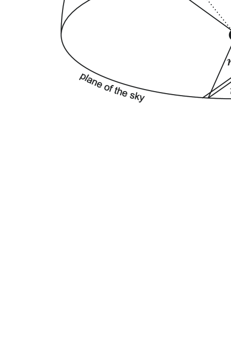
Figure 1: The meaning of the different kinds of angular elements

2.2 The contributions of Eclipse Timing Variations

We define the general form of the ETV as follows:

$$\Delta = T(E)-T(0)-P_{\mathrm{s}}E$$ (1)

$$= \sum_{i=0}^{2}c_{i}E^{i}+\left[\Delta_{\mathrm{LTTE}}+\Delta_{\mathrm{dyn}}+\Delta_{\mathrm{apse}}\right]_{0}^{E},$$

where, on the first row, $T(E)$ denotes the observed time of the $E$-th eclipse, $T(0)=T_{0}$ indicates the reference epoch, i.e., the observed time of the “zeroth” eclipse, while the constant $P_{\mathrm{s}}$ stands for the sidereal (or eclipsing) period. Furthermore, the $c_{0}$, $c_{1}$ coefficients give corrections in $T_{0}$ and $P_{\mathrm{s}}$, respectively, while $c_{2}$ is equal to half of the constant period-variation rate per cycle ($\Delta P/2$), independent of its origin. Finally, $\Delta_{\mathrm{LTTE}}$, $\Delta_{\mathrm{dyn}}$ and $\Delta_{\mathrm{apse}}$ refer to the contributions of light-travel time effect (LTTE), short period dynamical perturbations, and apsidal motion effect (AME, including longer time-scale dynamical perturbations) to the ETVs, respectively. Note, the integer values of cycle number $E$ refer to the primary, and half-integers to the secondary eclipses. In the following we briefly discuss each of the above mentioned components.

(i) Light Travel Time effect (LTTE): This is the classical Roemer delay that arises from the changing distance of the eclipsing binary from the observer during its revolution around the center of mass (CM) of the triple system. This effect is well-observed in hundreds of eclipsing systems. LTTE is a close analog of the Doppler shift in the radial velocities in binaries. It produces exactly the same information which can be obtained from an SB1 radial velocity curve. It can be written as

$$\Delta_{\mathrm{LTTE}}=-\frac{a_{\mathrm{AB}}\sin i_{2}}{c}\frac{\left(1-e_{2}^{2}\right)\sin(v_{2}+\omega_{2})}{1+e_{2}\cos v_{2}},$$ (2)

Note, the negative sign on the r.h.s. comes from the fact that in the LTTE-term the motion of the binary is reflected, and we applied the relation $\omega_{\mathrm{AB}}=\omega_{2}+180\degr$. By the use of Kepler’s third law, the mass function can be defined as

$$f(m_{\mathrm{C}})=\frac{m_{\mathrm{C}}^{3}\sin^{3}i_{2}}{m_{\mathrm{ABC}}^{2}}=\frac{4\pi^{2}a_{\mathrm{AB}}^{3}\sin^{3}i_{2}}{GP_{2}^{2}}$$ (3)

and thus, the amplitude of LTTE can be written as

$${\cal{A}}_{\mathrm{LTTE}} = \frac{G^{1/3}}{c}\left(\frac{P_{2}}{2\pi}\right)^{2/3}f(m_{\mathrm{C}})^{1/3}\sqrt{1-e_{2}^{2}\cos^{2}\omega_{2}}$$ (4)

$$\approx 1.1\times 10^{-4}\frac{m_{\mathrm{C}}\sin i_{2}}{m_{\mathrm{ABC}}^{2/3}}P_{2}^{2/3}\sqrt{1-e_{2}^{2}\cos^{2}\omega_{2}},$$

where, in the last row, masses are given in units of $M_{\odot}$, the period in days, and the amplitude is also expressed in days.

The LTTE term carries information about the following parameters: $P_{2}$, $e_{2}$, $\omega_{2}$, $\tau_{2}$ (or its equivalents), and the projected semi-major axis $a_{\mathrm{AB}}\sin i_{2}$ or, the mass function $f(m_{\mathrm{C}})$.

(ii) $P_{2}$ time-scale dynamical effects: This is the medium of the three classes of periodic perturbations (both in amplitude, and period) in hierarchical triple configurations. Such perturbations in the context of eclipse timing variations were first analyzed by Söderhjelm (1975), and Mayer (1990). Later, a corrected and easily applicable form was given in Borkovits et al. (2003) which was adequate insofar as the inner binary had a circular orbit and, furthermore, the third companion was sufficiently distant that terms of higher order than quadruple of the perturbing potential (or force) would be negligible. Rappaport et al. (2013) successfully applied the combination of LTTE and their dynamical model for the identification and preliminary orbital parameter determination of 39 close hierarchical triple systems amongst Kepler eclipsing binary stars. A natural extension of the previous model for eccentric inner binaries was carried out by Borkovits et al. (2011). For eccentric inner binaries the equations (up to the first order in the $a_{1}/a_{2}$ ratio) take the following form:

$$\Delta_{\mathrm{1}} = \frac{P_{1}}{2\pi}A_{\mathrm{L1}}\left(1-e_{1}^{2}\right)^{1/2}\left\{\left[\frac{8}{15}f_{1}+\frac{4}{5}K_{1}\right]\right.{\cal{M}}$$ (5)

$$+\left(1+I\right)\left[K_{11}{\cal{S}}(2u_{2}-2\alpha)-K_{12}{\cal{C}}(2u_{2}-2\alpha)\right]$$

$$+\left(1-I\right)\left[K_{11}{\cal{S}}(2u_{2}-2\beta)+K_{12}{\cal{C}}(2u_{2}-2\beta)\right]$$

$$+\sin^{2}i_{\mathrm{m}}\left(K_{11}\cos 2n_{1}+K_{12}\sin 2n_{1}\right.$$

$$\left.\left.-\frac{2}{5}f_{1}-\frac{3}{5}K_{1}\right)\left[2{\cal{M}}-{\cal{S}}(2u_{2}-2n_{2})\right]\right\}$$

$$+\Delta_{1}^{*}(\sin i_{\mathrm{m}}\cot{i_{1}}),$$

where the dimensionless, $P_{2}$ (i.e., long-) timescale dynamical amplitude is

$$A_{\mathrm{L1}}=\frac{15}{8}\frac{m_{\mathrm{C}}}{m_{\mathrm{ABC}}}\frac{P_{1}}{P_{2}}\left(1-e_{2}^{2}\right)^{-3/2},$$ (6)

while

$${\cal{M}} = v_{2}-l_{2}+e_{2}\sin v_{2},$$

$${\cal{S}}(2u_{2}) = \sin{2u_{2}}+e_{2}\left[\sin(u_{2}+\omega_{2})+\frac{1}{3}\sin(3u_{2}-\omega_{2})\right],$$

$${\cal{C}}(2u_{2}) = \cos{2u_{2}}+e_{2}\left[\cos(u_{2}+\omega_{2})+\frac{1}{3}\cos(3u_{2}-\omega_{2})\right].$$

Furthermore,

$$f_{1} = 1+\frac{25}{8}e_{1}^{2}+\frac{15}{8}e_{1}^{4}+\frac{95}{64}e_{1}^{6}+{\cal{O}}(e_{1}^{8}),$$ (8)

$$K_{1} = \mp e_{1}\sin\omega_{1}+\frac{3}{4}e_{1}^{2}\cos 2\omega_{1}+{\cal{O}}(e_{1}^{3}),$$ (9)

$$K_{11} = \frac{3}{4}e_{1}^{2}\pm e_{1}\sin\omega_{1}+\frac{51}{40}e_{1}^{2}\cos 2\omega_{1}+{\cal{O}}(e_{1}^{3}),$$ (10)

$$K_{12} = \mp e_{1}\cos\omega_{1}+\frac{51}{40}e_{1}^{2}\sin 2\omega_{1}+{\cal{O}}(e_{1}^{3}).$$ (11)

The functions $K_{n}(e_{1},\omega_{1})$ are also given up to higher orders in $e_{1}$ in Eqs. (43) of Appendix A. It is important to bear in mind that, in these formulae and throughout this paper, $\omega_{i}$’s are used in the sense of the argument of periastron of the secondary’s orbit relative to its primary. With such a choice, the upper signs represent primary minima. Finally, $\Delta_{1}^{*}(\sin i_{\mathrm{m}}\cot{i_{1}})$ stands for the terms which arise directly from the nodal precession for non-coplanar systems. As these terms are multiplied by $\cot{i_{1}}$ they give a substantially smaller contribution for eclipsing binary systems seen nearly edge on. For the sake of completeness, however, we retained and included these terms in the analysis. They are given in Eq. (42) of Appendix A.

Equation (5) is equivalent to Eq. (B.15) of Borkovits et al. (2011). However, the use of true longitude ($u_{2}$), and node-like azimuthal angles ($n_{1}$, $n_{2}$) instead of true anomaly ($v_{2}$) and dynamical argument of periastrons ($g_{1}$, $g_{2}$), as was done previously, has the advantage that, in such a way, Eq. (5) remains valid even for the special cases of circular orbits, and for coplanar configurations as well. (For this latter case we note that, although $n_{1}$ and $n_{2}$ have no meaning for coplanar orbits, it can be easily seen that for $i_{\mathrm{m}}\rightarrow 0\degr$ $\alpha\rightarrow 0\degr$, and for $i_{\mathrm{m}}\rightarrow 180\degr$ $\beta\rightarrow 180\degr$ and thus, the non-vanishing components of Eq. [5] really retain their well defined meanings.)

These terms yield information on the mass-ratio $m_{\mathrm{C}}/m_{\mathrm{ABC}}$, and (either directly, or indirectly) on the orbital elements of both the inner and the outer orbits. This includes angles referring to both the celestial (or observational) and the relative (or dynamical) frames of reference, namely: $P_{1}$, $e_{1}$, $\omega_{1}$, $P_{2}$, $e_{2}$, $\omega_{2}$, $\tau_{2}$, $i_{\mathrm{m}}$ and (via the node-like angles $n_{1}$ and $n_{2}$), $\Delta\Omega$, $g_{1}$, $g_{2}$, $h_{1}$, $h_{2}$, and furthermore, theoretically, even on all the observable ($i_{1}$, $i_{2}$) and dynamical inclinations (i.e., orbital inclinations relative to the fundamental plane of the system, $j_{1}$, $j_{2}$). Finally, the inclination of the invariable plane relative to the plane of the sky ($i_{0}$) can also be determined and therefore, the complete spatial configuration can be inferred as well. For all these calculations, and therefore for the entire orbital parameter fitting process, the spherical triangle(s) formed by the two orbital planes and the plane of the sky on the celestial sphere, and also its two constituents, i.e., the analogous triangles formed by one or the other of the orbital planes with the invariable plane and the sky (see Fig. 1), have fundamental importance. A thorough discussion of these spherical triangles including all the possible information to extract in all possible configurations is given in Appendix D.

Some of the recently discovered Kepler-triples that we have investigated were found to be such compact systems that we have decided to include additional terms which are second order in the $a_{1}/a_{2}$ ratio. These contributions occur when the octupole term of the perturbing potential function (or its equivalent perturbing force components) are included. In order to improve our model with these contributions, we used a similar method to that for the case of the quadruple approximation in our previous work. Therefore, we do not include the calculations here. The complete formula is so lengthy that it is given only in Eq. (38) of Appendix A. At this point we discuss only some general properties, and describe a few special cases, where the expressions become substantially simpler.

The amplitude of the second order term is

$$A_{\mathrm{L2}}=\frac{1-q_{1}}{1+q_{1}}\left(1-\frac{m_{\mathrm{C}}}{m_{\mathrm{ABC}}}\right)^{1/3}\left(\frac{P_{1}}{P_{2}}\right)^{2/3}\frac{A_{\mathrm{L1}}}{1-e_{2}^{2}},$$ (12)

which reveals, that this term introduces one additional parameter, which is the mass ratio of the inner binary ($q_{1}$). Furthermore, when $q_{1}$ tends to be unity (i.e., the two components of the inner binary tend to have equal masses), the octupole terms tend to be zero. As will be discussed later, despite the relatively small contribution of the octupole terms to the whole ETV, the resultant mass ratios were found, in most cases, to be in qualitative accord with the expected values. By this we mean that for systems exhibiting more or less similarly deep primary and secondary eclipses, the resultant mass ratios were found to be near unity, while in cases of highly unequal eclipse depths, smaller mass ratios were obtained.

For a coplanar configuration, the equations reduce significantly. For such a scenario Eq. (5) simplifies to

$$\Delta_{1}^{\mathrm{pro}} = \frac{1}{2\pi}\frac{m_{\mathrm{C}}}{m_{\mathrm{ABC}}}\frac{P_{1}^{2}}{P_{2}}\frac{\left(1-e_{1}^{2}\right)^{1/2}}{\left(1-e_{2}^{2}\right)^{3/2}}\left[\left(1\mp\frac{3}{2}e_{1}\sin\omega_{1}\right){\cal{M}}\right.$$

$$\left.\pm 2e_{1}{\cal{C}}(2u_{2}-\omega_{1})\right]+{\cal{O}}(e_{1}^{2}),$$

$$\Delta_{1}^{\mathrm{ret}} = \frac{1}{2\pi}\frac{m_{\mathrm{C}}}{m_{\mathrm{ABC}}}\frac{P_{1}^{2}}{P_{2}}\frac{\left(1-e_{1}^{2}\right)^{1/2}}{\left(1-e_{2}^{2}\right)^{3/2}}\left[\left(1\mp\frac{3}{2}e_{1}\sin\omega_{1}\right){\cal{M}}\right.$$ (13)

$$\left.\mp 2e_{1}{\cal{C}}(2u_{2}+\omega_{1})\right]+{\cal{O}}(e_{1}^{2})$$

for prograde and retrograde configurations, respectively. In the same case the octupole term, i. e. Eq. (38) takes the following form:

$$\Delta_{2}^{\mathrm{pro}} = \frac{P_{1}}{2\pi}A_{\mathrm{L2}}\left(1-e_{1}^{2}\right)^{1/2}\left[\mp{\cal{C}}_{21}(u_{2})\right.$$

$$-e_{1}\cos\omega_{1}{\cal{S}}_{21}(u_{2})-\frac{57}{20}e_{1}{\cal{S}}_{21}(u_{2}-\omega_{1})$$

$$\left.-\frac{1}{4}e_{1}{\cal{S}}_{21}(u_{2}-3\omega_{1})\right]+{\cal{O}}(e_{1}^{2}),$$

$$\Delta_{2}^{\mathrm{ret}} = \frac{P_{1}}{2\pi}A_{\mathrm{L2}}\left(1-e_{1}^{2}\right)^{1/2}\left[\mp{\cal{C}}_{21}(u_{2})\right.$$ (14)

$$+e_{1}\cos\omega_{1}{\cal{S}}_{21}(u_{2})+\frac{57}{20}e_{1}{\cal{S}}_{21}(u_{2}+\omega_{1})$$

$$\left.+\frac{1}{4}e_{1}{\cal{S}}_{21}(u_{2}+3\omega_{1})\right]+{\cal{O}}(e_{1}^{2}).$$

A further reduction of this situation for a circular inner orbit leads to the approximation used by Agol et al. (2005). (Note, these authors considered the first order, or quadrupole terms only.)

Second, if both orbits are circular, but the orbital planes are inclined, Eqs. (5) and (38) reduce to

$$\Delta_{1} = \frac{3}{8\pi}\frac{m_{\mathrm{C}}}{m_{\mathrm{ABC}}}\frac{P_{1}^{2}}{P_{2}}\sin^{2}i_{\mathrm{m}}\sin(2u_{2}-2n_{2}),$$ (15)

$$\Delta_{2} = \pm\frac{P_{1}}{4\pi}A_{\mathrm{L2}}\left\{\left[(1-I)\cos(u_{2}-\beta)\right.\right.$$ (16)

$$\left.-(1+I)\cos(u_{2}-\alpha)\right]$$

$$+\frac{5}{2}\sin^{2}i_{\mathrm{m}}\left\{(1+I)\left[\cos(u_{2}-\alpha)\right.\right.$$

$$\left.+\frac{1}{2}\cos(u_{2}-\beta)-\frac{1}{2}\cos(3u_{2}-2\alpha-\beta)\right]$$

$$-(1-I)\left[\cos(u_{2}-\beta)+\frac{1}{2}\cos(u_{2}-\alpha)\right.$$

$$\left.\left.\left.-\frac{1}{2}\cos(3u_{2}-2\beta-\alpha)\right]\right\}\right\}.$$

Insofar as we consider only the first order approximation (Eq. 15), one can see that in this case the dynamical term has a unique period of $1/2P_{2}$; therefore, this is the only scenario where the LTTE and dynamical perturbation are clearly separable in Fourier-space. In the coplanar and circular binary cases, however, the first order dynamical contribution vanishes. This situation occurs in the triply eclipsing system HD 181068 (Borkovits et al., 2013). By contrast, in the octuple approximation, even in this latter scenario, there remains a small amplitude, non-zero contribution with period equal to $P_{2}$, as long as the inner binary members have unequal masses. Moreover, the octupole terms result in a small phase displacement, and might also break the degeneracy between the primary and secondary eclipses even in (originally) circular cases.

Finally, we note that the dimensionless dynamical amplitudes in the ETV functions considered above scale with the inner binary’s orbital period ($P_{1}$), and take on their time dimensions in the following form:

$${\cal{A}}_{\mathrm{L1,L2}}=\frac{P_{1}}{2\pi}A_{\mathrm{L1,L2}}.$$ (17)

(iii) $P_{2}$ time-scale residuals of the $P_{1}$ time-scale dynamical effects: For most of the systems, investigated in this paper, the $P_{1}/P_{2}$ ratio is between $10^{-1}$ and $10^{-2}$ and, therefore the amplitude of the shortest period perturbations may reach nearly 10% of the longer period ones and, therefore, their effects should also be considered. These perturbations, however, due to our natural sampling process in the eclipse minima, will also produce additional, smaller amplitude, $P_{2}$ time-scale terms. The highly simplified, approximate nature of the way they are calculated is discussed in Appendix B. The somewhat lengthy complete form of this perturbative term is also given there.

The dimensionless amplitude of these terms becomes

$$A_{\mathrm{S}}=\frac{P_{1}}{P_{2}}\frac{A_{\mathrm{L1}}}{\left(1-e_{2}^{2}\right)^{3/2}},$$ (18)

which, in the ETV curves, scales as

$${\cal{A}}_{\mathrm{S}}=\frac{P_{1}}{2\pi}A_{\mathrm{S}}.$$ (19)

For coplanar configuration we obtain that

$$\Delta_{\mathrm{S}}^{\mathrm{pro}} = \frac{P_{1}}{\pi}A_{\mathrm{S}}\left(1-e_{1}^{2}\right)^{1/2}(1+e_{2}\cos{v_{2}})^{3}\left\{-\frac{11}{30}\sin(2u_{2})\right.$$

$$\pm e_{1}\left[\cos\omega_{1}+\frac{4}{5}\cos(2u_{2}-\omega_{1})\right.$$

$$\left.\left.+\frac{8}{15}\cos(2u_{2}+\omega_{1})\right]\right\}+{\cal{O}}[e_{1}^{2},(P_{1}/P_{2})^{3}],$$

$$\Delta_{\mathrm{S}}^{\mathrm{ret}} = \frac{P_{1}}{\pi}A_{\mathrm{S}}\left(1-e_{1}^{2}\right)^{1/2}(1+e_{2}\cos{v_{2}})^{3}\left\{\frac{11}{30}\sin(2u_{2})\right.$$ (20)

$$\pm e_{1}\left[\cos\omega_{1}+\frac{4}{5}\cos(2u_{2}+\omega_{1})\right.$$

$$\left.\left.+\frac{8}{15}\cos(2u_{2}-\omega_{1})\right]\right\}+{\cal{O}}[e_{1}^{2},(P_{1}/P_{2})^{3}],$$

while the non-coplanar, doubly circular scenario results in

$$\Delta_{\mathrm{S}} = \frac{11}{32\pi}\frac{m_{\mathrm{C}}}{m_{\mathrm{ABC}}}\frac{P_{1}^{3}}{P_{2}^{2}}\left\{-(1+I)\sin(2u_{2}-2\alpha)\right.$$ (21)

$$+(1-I)\sin(2u_{2}-2\beta)$$

$$\left.-\sin^{2}i_{\mathrm{m}}\sin 2n_{1}[1+\cos(2u_{2}-2n_{2})]\right\}$$

$$+{\cal{O}}[(P_{1}/P_{2})^{3}]$$

The above equations reveal that if the third star is close enough, even the quadrupole approximation can result in a significant non-vanishing component in the doubly circular, coplanar case, with period of $P_{2}/2$. Furthermore, as will be discussed, the inclusion of these terms substantially improved our fits in the low-amplitude mutual inclination regime, even in the case where both the inner and outer orbits had significant eccentricity.

(iv) Apse-node time-scale effects: In the case of an eccentric eclipsing binary, the orientation of the orbit with respect to the observer strongly affects the orbital phase and, therefore, the time when eclipses occur. The apsidal motion contribution to the ETV can be calculated from Kepler’s equation in a straightforward manner and, although it is usually given in a trigonometric series of $\omega_{1}$ (see e.g. Giménez & Garcia-Pelayo, 1983), it has an exact, analytical form, as follows:

$$\Delta_{\mathrm{apse}} = \frac{P_{1}}{2\pi}\left[2\arctan\left(\frac{\pm e_{1}\cos\omega_{1}}{1+\sqrt{1-e_{1}^{2}}\mp e_{1}\sin\omega_{1}}\right)\right.$$ (22)

$$\left.\pm\sqrt{1-e_{1}^{2}}\frac{e_{1}\cos\omega_{1}}{1\mp e_{1}\sin\omega_{1}}\right],$$

Apsidal motion studies of eccentric eclipsing binaries have been carried out for more than 75 years (see Cowling, 1938; Sterne, 1939). In all the previously observed systems the apsidal motion has arisen from the tidally deformed (i.e., oblate) stellar shapes, and/or from relativistic effects. There were no systems involving non-degenerate stars, however, where forced apsidal motion due to dynamical perturbations was previously detected. (On the other hand, the perturbing effects of an unseen third body have been suggested for explaining the anomalously slow apsidal motion of a few binaries, see e.g., Khaliullin et al., 1991, for DI Her, and Khodykin & Vedeneyev, 1997, for AS Cam. Note, that even for these two systems, recent investigations have shown that the origin of the unexpectedly slow apsidal motion may be explained by the misalignment of the spin axes, instead of the effects of a third body (see Albrecht et al., 2009; Pavlovski et al., 2011, for the two systems, respectively).

In the case of relativistic apsidal motion the apsidal line rotates with a constant angular velocity in the direction of the orbital motion. “Pseudo-synchronously” rotating oblate stars with negligible, or weak tidally induced oscillations also produce similar kinds of apsidal motion. Therefore, for most of the previously known binaries we can simply write that

$$\omega_{1}(E)=\omega_{1}(0)+\Delta\omega_{1}E,$$ (23)

where $\Delta\omega_{1}$ denotes the apsidal advance rate for one orbital period, and therefore, the apsidal motion contribution to the ETV can be modeled in a simple way by substituting Eq. (23) into (22).

For third-body forced apsidal motion, the situation is substantially more complicated. In this case, in general, none of the orbital parameters (except the semi-major axes) remains constant. It is especially true for high mutual inclination systems with negligible tidal oblateness, where an initially very low, or even zero eccentricity may grow up to near unity. (This is the so-called Kozai-Lidov mechanism, which have been investigated and discussed in several recent papers, see e.g. Naoz et al., 2013, and further references therein.)

In this paper, however, we leave out a rigorous consideration of such a scenario, and restrict ourselves to the case where the variation in the inner eccentricity is small, or negligible. (We will verify this choice in the discussion.) This situation was elaborately investigated by Borkovits et al. (2007), where references to previous works were also given. For the sake of completeness, the basic steps, and additional discussion are included in Appendix C.

In this simplified approach the apsidal motion was modeled in three different ways: (i) the apsidal advance rate $\Delta\omega_{1}$ (or $\dot{\omega}_{1}$) is taken to be an unconstrained constant which is an adjustable additional parameter of the solution; or (ii) $\dot{\omega}_{1}$ is a constrained constant whose numerical value is calculated from other system parameters according to Eq. (55); or (iii) $\dot{\omega}_{1}$ is no longer considered to be constant, but a time-dependent quantity. In this third case we have no need to calculate $\dot{\omega}_{1}$ (or $\Delta\omega_{1}$), because the instantaneous value of $\omega_{1}$ can be directly calculated from the time-dependent value of the dynamical apse and node $g_{1}$, $h_{1}$ via the approximate quadrupole analytic model that is described in Appendix C.

Because some of our systems exhibit rapid eclipse depth variations, which are a clear indicator of the varying inclination angle of the inner binary due to precession of its orbital plane, we also modeled this effect. This phenomenon does not influence the ETVs in a similarly expressive way as for apsidal motion. Its direct contribution to the ETVs is multiplied by $\cot i_{1}$ and, therefore, becomes negligible for our nearly edge-on systems. On the other hand, apsidal motion substantially affects the dynamical apsidal motion rates, and also the $n_{1,2}$ node-like quantities. Another significant contribution of its effect to the ETVs comes from the variations of the $n_{1}$ and $n_{2}$ angles which appear explicitly in the $P_{2}$ period dynamical terms ($\Delta_{1}$, $\Delta_{2}$). In modeling the orbital precession, we applied the same approximations as in the case of apsidal motion. Specifically, in the case of a constant apsidal motion rate, the nodal regression (or progression) rate ($\Delta h$) was also considered to be constant, being either unconstrained, or constrained with a value obtained from Eq. (54), and was substituted into the equation

$$h(E)=h(0)-\Delta hE,$$ (24)

or, when $\omega_{1}$ was calculated according to the first order analytic solution, the same was done for $h_{1}$. (A detailed description is given in Appendix C.) Then, when the actual value of the dynamical node ($h$) for cycle number $E$ was calculated, the corresponding $n_{i}$’s were computed using the theorems of spherical triangles. The straightforward calculation, and its not-so-straightforward discussion, are given in Appendix D.

Equation (22) provides very strong constraints on $e_{1}\cos\omega_{1}$ and, especially for the shorter-period apsidal motion systems (i.e., where a relatively larger portion of a complete cycle is covered), on the apsidal motion period as well. Furthermore, this period provides further constraints on the following parameters: $e_{1}$, $g_{1}$, $e_{2}$, $i_{\mathrm{m}}$, $P_{1}/P_{2}$ as well as, via the apsidal motion period, the mass ratio $m_{\mathrm{C}}/m_{\mathrm{ABC}}$, thereby establishing a connection between the amplitude of the $P_{2}$-period dynamical perturbations and the apsidal motion (and orbital precession) periods. These provide important additional constraints for a physically reliable solution.

The orbital precession terms have lesser direct influence due to their moderate contribution to the ETVs; however, there is a strong connection among the rate and amplitude of the eclipse depth variations and the precession rate, the mutual inclination, and the relative orientation of the orbits with respect to the observer (as is discussed in Appendices C and D). Later, in Sect. 5 we use these connections to verify or reject certain ETV solutions, or to choose between alternative, ambiguous solutions of the same triples.

(iv) Other, small effects: There are several additional, usually negligibly small amplitude effects, two of which we nonetheless mention.

First is the intrinsic light-travel-time effect for the two components of the inner binary. For short (few-day) period eclipsing binaries, which form the large majority of EBs discovered incidentally by astronomers in previous centuries, its effect, due to the small orbital separation, remains below the accuracy of ground-based timing measurements. However, for longer period eclipsing binaries, observed especially with the accuracy of Kepler photometry this effect becomes detectable. Therefore, as far as we know, this may be the reason why this effect was not considered before the Kepler era. A simplified form for circular orbits was first used by Kaplan (2010), while the general, eccentric form is given in Fabrycky (2010). These papers, however give only the differential form of the effect, i.e., the displacement of the secondary eclipses with respect to the primary eclipses. Here we list the formula separately for the two types of eclipses:

$$\Delta_{\mathrm{LTTEin}}=\pm\frac{1}{c}\frac{q_{1}-1}{q_{1}+1}\frac{a_{1}\sin i_{1}\left(1-e_{1}^{2}\right)}{1\mp e_{1}\sin\omega_{1}}.$$ (25)

The other small effect is due to the slight inclination ($i_{1}$) dependence of the occurrences of the eclipse events for eccentric orbits. This effect was discussed in detail by Giménez & Garcia-Pelayo (1983), for example. These authors also gave the mathematical form of the ETVs due to apsidal motion with the extension of this inclination dependence. These formulae are in use up to the present time. For a recent paper on this topic see Wolf et al. (2013). However, this effect can be included into our equations by simply redefining the observable argument of periastron formally as follows:

$$\omega_{1}^{*}=\omega_{1}\mp\frac{e_{1}\cos\omega_{1}\cos^{2}i_{1}}{\sin^{2}i_{1}\mp e_{1}\sin\omega_{1}},$$ (26)

which is the first order approximation of Eq. (10) of Giménez & Garcia-Pelayo (1983).

(v) Other effects, not taken into account: We have left out of the present considerations the changes or perturbations in the outer orbital elements. This was done for two reasons. First, the amplitudes of the variations in the outer orbital elements for hierarchical systems usually remain much lower than those of the inner orbital elements (see, e.g. Harrington, 1968, 1969). Furthermore, the perturbations in the outer elements affect the binary motion and, therefore the ETV curves, in an indirect way which would appear only in higher-order approximations. Despite this, as a forthcoming step, we plan the inclusion of these terms for a better modeling of the most compact triples.

We also omitted those apsidal motion and orbital precession effects which would arise from tidal or relativistic interactions. In Sect. 5, in light of our results, we justify this decision. The tidal effects, however, are discussed briefly in Appendix C.

Finally, we also neglected the octupole “apse-node” timescale perturbation terms. Our experience from the present study is that these latter terms certainly have to be included for better future modeling of the most compact systems.

3 Analysis code

In the parameter search for the sample of 26 hierarchical triple systems studied in this work we departed from the method followed in the previous study of Rappaport et al. (2013). In that paper it was stated that due to the strong and highly nonlinear correlations between several parameters, the conventional Levenberg-Marquardt (LM) fitting procedure was not adequate for the exploration of the parameter phase space. The main source of this difficulty originated from the non-orthogonality of the two functions describing the LTTE and the dynamical terms, which each contributed ETV curves that could be more or less comparable in magnitude and shape, for their sample of CHTs. In contrast, in our current collection of eccentric triples, the $P_{2}$ time-scale quadrupole dynamical terms highly dominate over all the other contributors for all systems. Furthermore, the inclusion of additional relations and information allows for strict constraints to be set on some of the combinations of parameters and, therefore, reduces the degeneracies. Here we refer, e.g., to the connections between the different inclination and node-like parameters (which provide additional constraints on even the dynamical angular elements and the masses), and the apsidal motion terms, the latter of which very strictly constrain not only the $e_{1}\cos\omega_{1}$-term, but in the cases of several systems, both $e_{1}$ and $\omega_{1}$ individually, and finally the outer mass ratio. Therefore, we decided to apply a combination of the LM fitting procedure and a grid-search method in our parameter adjustment process.

In its present state, the code contains 20 adjustable parameters; however, because of the different kinds of interconnections we do not allow for the adjustment of all these parameters in the same run. (For example, from the six angles and node-like arcs of the spherical triangle discussed in Appendix D, only three are allowed to be included in the fitting process.) There are some additional flags which choose the actual working mode of the code (i.e., which terms to be included, or not, and which additional constraints to be applied, or not). The adjustable parameters, collecting them into five groups, are as follows:

1. $V_{\gamma}$ – systemic radial velocity (not used in this work)

2. $c_{0}$, $c_{1}$, $c_{2}$ – coefficients of the polynomial contribution which are used in part for determining the refined value of the epoch $T_{0}$ and sidereal period $P_{\mathrm{s1}}$. The fitting of the quadratic coefficient $c_{2}$ can be, and was, disabled for all but one of the runs presented here.

3. $e_{1}$, $\omega_{1}$, $\Delta\omega_{1}$ (the last of which, i.e., the apsidal advance rate, may be either unconstrained, or calculated according to one of the two methods as discussed)

4. $a_{\mathrm{AB}}\sin{i_{2}}$, $a_{\mathrm{C}}\sin{i_{2}}$, $P_{2}$, $e_{2}$, $\omega_{2}$, $\tau_{2}$, $q_{1}$ – or, optionally, some physical (but not numerical) equivalents, e.g., the mass function, $f(m_{\mathrm{C}})$, and mass ratio, $m_{\mathrm{C}}/m_{\mathrm{ABC}}$.

5. $i_{\mathrm{m}}$, $i_{1}$, $i_{2}$, $n_{1}$, $n_{2}$, $\Delta{h}$ (where two from the first five are computed from the other three, while the orbital precession rate may be either unconstrained, or calculated in a similar manner, as was discussed for the apsidal advance)

During a fitting run session one of the following six possibilities was applied for each of the parameters: it was (i) kept fixed at its initial value; (ii) kept fixed at different, equally spaced initial values (grid search); (iii) adjusted by the LM process, starting from a single initial value; (iv) LM-adjusted, starting from several equally spaced initial values; (v) calculated (constrained) from other parameters; or (vi) not considered, according to the respective model. A detailed description of the code will be presented elsewhere in a technical paper; here we discuss only that part which is relevant for the present work.

In order to check the analytical formulae on one hand, and the numerical behavior of our parameter adjustment process, as well as the uniqueness of the solutions, on the other hand, we have carried out various tests. Basically, these investigations have two separate parts. First, we obtained solutions for actual Kepler ETV curves by utilizing different model approximations. Then the solutions that were obtained were used as initial parameters for a 3-body numerical integration from which we generated the associated artificial ETV curves. We then compared these to the actual, observed ETVs. The consistency of this loop is a direct measure of how good the solution is. Second, we obtained fitted solutions for these numerically generated ETVs, and compared the solution parameters with the known initial values. Furthermore, we have also varied some of the input parameters to check the solutions’ behavior and dependence upon some of the model parameters. Moreover, the same test runs were used to check the reliability of the formal errors calculated from the covariance matrices of the LM-solutions with the empirical rms scatter in the different solutions we investigated.

It is clear, however, that despite the speed and effectiveness of this method for exploring how well the analytic fits work, it has some inevitable disadvantages. In particular, the LM portion of the fits does not explore non-ellipsoidal correlations in multi-dimensional $\chi^{2}$ space, while the grid portion of the search excludes certain physically unrealistic regions of parameter space. Therefore, instead of automatically accepting the formal errors obtained from our fits, we use the solutions recovered from the numerically generated ETVs with known parameters to demonstrate the overall reliability of our methods, and for the estimation of more conservative uncertainties for some of the parameters. In Appendix E we discuss the steps of the complete investigation for a few systems in detail, which also provides us some insight into the methodology of the analysis.

Table 2: Properties of the investigated systems

KIC No.	$P_{\mathrm{s1}}$	$T_{0}$	$K_{\mathrm{p}}$	$T_{\mathrm{eff}}$	$\log{g}$	$P_{2}/P_{1}$	Ecl.depths	Tertiary
	(days)	(MBJD)	(mag)	(K)			variation	eclipses
04940201a	8.816578	54967.276926	14.98	5284	4.61	41.4	…	…
05255552	32.448635	54970.636491	15.21	4775	4.59	26.5	(j+)	yes
05653126	38.493382	54985.913152	13.17	5766	3.81	25.1	+a2	…
06545018a	3.991460	54965.835642	13.75	5594	4.46	22.7	…	…
07289157a	5.266425	54969.966600	12.95	6013	4.19	46.2	-	yes
07812175	17.793925	55002.612666	16.33	NA	NA	32.7	NA	…
08023317a	16.579002	54979.733478	12.89	5625	4.05	36.8	+	…
08210721	22.672816	54971.157082	14.27	5412	4.28	34.8	…	…
08938628a	6.862216	54966.603088	13.68	5602	4.29	56.6	c-	…
09714358a	6.474177	54967.395501	15.00	4825	4.55	16.02	…	…
05771589a	10.739142	54962.130765	11.81	5927	4.23	10.5	-+	…
06964043	5.362659	55291.992805	15.61	5374	4.44	22.3	+-	yes
07668648a	27.818590	54963.315401	15.32	5875	4.52	7.3	+,x	yes
07955301a	15.326340	54967.950750	12.67	4821	3.12	13.6	+c,x	…
04769799	21.929314	54968.505532	10.95	4911	3.57	56.1	j-;d2	…
05003117	37.613001	54986.092638	14.03	5387	4.49	57.2	c(-)	…
05731312	7.946382	54968.093163	13.81	4658	4.49	114.1	(j-)	…
07670617	24.703160	54969.139216	15.52	4876	4.73	130.9	j-	…
08143170	28.785943	54970.113064	12.85	4957	3.68	59.4	(c+)	…
09715925	6.308199	54998.939653	16.52	4891	4.46	116.7	c+	…
09963009	40.069657	54986.018248	14.46	5653	4.33	94.1	c-2	…
10268809	24.708999	54971.999951	13.74	5787	4.42	283.3	j-;x	…
10319590a	21.320459	54965.716743	13.73	5518	4.37	21.1	-d	…
10979716	10.684056	54967.082259	15.77	3932	4.61	97.8	…	…
11519226	22.160715	54973.018008	13.03	5646	4.54	64.6	…	…
12356914	27.307455	54976.508322	15.53	5368	4.58	66.5	…	…

Notes. (1) Sidereal period ($P_{\mathrm{s1}}$) and epoch ($T_{0}$) were used for plotting $O-C$ curves. $T_{0}$ was also used as reference epochs for most of the parameters listed in Tables 3–5. (The exceptions are noted in each table.) (2) Kepler magnitude, effective temperature and $\log g$ were taken from the Kepler Input Catalog. (3) Further notes for column ‘KIC numbers’: $a$: listed in Rappaport et al. (2013) – for column ‘eclipse depth variations’: +/-: continuous increase/decrease; j: sudden jump; c: constant (marked only if the eclipse depth remains constant during a portion, but not the whole time-span, of the observations); a2/d2: appearance/disappearance of secondary eclipses; d: eclipses disappeared; x: exchange of the amplitudes in primary/secondary eclipses; (marks in parenthesis): slight/uncertain variation; … : no eclipse depth variation.

4 System selection and data preparation

The present version of the Kepler Eclipsing Binary Catalog (Conroy et al., 2014) contains 2645 EBs. We selected our systems from that sample. We started our search for the appropriate CHTs with the construction of $O-C$ (‘observed minus calculated’ eclipse times) curves for the primary and, when possible, the secondary, eclipses for all 2645 binaries. At the same time we also produced folded light curves for each binary. In all, we found some 400 binary systems that have interesting (i.e., non-linear) $O-C$ curves (see also Rappaport et al. 2013; Conroy et al. 2014). However, most of these tend to be either parabolically shaped or have sinusoidal shapes with a period comparable to, or longer than, the Kepler mission. The majority of these are probably triple systems, as indicated by the presence of perturbations that are likely due to a third body in the system, but are otherwise not particularly interesting for the present study. We then restricted our attention only to the subset of these systems which satisfied the following three criteria:

• The inner eclipsing binary should have an eccentric orbit.

  A good indicator of an EB’s eccentricity in the light curve is the displacement of the secondary eclipse from the mid-time of two consecutive primary minima. For systems, however, with small eccentricity, and/or semi-major axes lying almost along the line of sight (i.e., $\omega_{1}\approx\pm 90\degr$), the eccentricity might go unnoticed. An equivalent sign of eccentricity in the $O-C$ curves occurs when the (averaged) primary and secondary $O-C$ curves do not overlap, or they even converge toward, or diverge from, each other (due to apsidal motion).

• The ETV curve should show clear signatures of third-body perturbations.

  These signatures can range from quasi-periodic modulations to relatively abrupt jumps in the ETV curves. Examples of both kinds will be shown later. Note, that light curves can also exhibit features which most likely come from a third component. These signs include (a) extra eclipses, especially when these extra events show definite variability in their shapes, and even in occurrences; (b) variations in the eclipse depths, which can be associated with the disappearance (or appearance) of one or the other or both eclipses, the change in the shape and duration of the eclipses, and even an exchange of the eclipse depths between the primary and secondary; or (c) a rapid variation of the time-lag between the primary and consecutive secondary eclipses.

• Both primary and secondary minima should have been observed, at least during a part of the Kepler mission.

  This last point is a technical requirement because, in the absence of secondary eclipses (and of course coupled with the lack of radial velocity measurements), we cannot constrain $e_{1}$, $\omega_{1}$ and $\Delta\omega_{1}$ from the apse-node timescale terms, and therefore, our solution would be strongly under-determined. There was only one supposed triple system, which was omitted according to this criterion. It was KIC 07837302 which was included in the paper of Rappaport et al. (2013). Note, that due to this requirement we did not check additional systems in the catalog which exhibit only one eclipse, therefore, we cannot exclude the presence of additional interesting triples amongst the EBs showing only one eclipse per orbit.

According to these criteria we first selected 10 EBs from the 39 systems investigated in Rappaport et al. (2013). We then made an extended search for other additional systems that fulfill our criteria. This included inspecting each of the 2645 ETV curves and associated folded light curves to find good candidates. Combining the results of these searches, we made a final selection of 26 systems for further analysis – of which the remaining 16 are newly reported here. The important parameters for these 26 hierarchical triples are listed in Table 2.

During the course of our analyses we realized that our sample should be divided into three subgroups, which are separated with two horizontal lines in the tables. The first group contains ten systems which were found to be the most ideal for our purposes, and therefore yielded the most reliable solutions. The four triples in the second group were found to be too close (i.e., quite compact) and therefore, our analytic fitting model was somewhat less satisfactory. For the remaining dozen systems, the largest uncertainties in the system parameters should arise from the insufficient Kepler coverage of the outer period. A detailed discussion is presented in Sect. 5.)

We used the entire Q0–17 long cadence (LC) datasets of Kepler eclipsing binaries. In order to have a unified treatment of the data, for the final runs we downloaded the complete, detrended LC light curves of all the selected systems from the Villanova site, and determined the times of minima and their uncertainties by the use of the first (BJD), seventh (detrended relative flux) and eighth (flux uncertainty) columns of these files.

Determination of Eclipse Times: The procedure for determining accurate eclipse times was done as follows. First, we calculated a phase-folded, binned and averaged light curve for each system. We found that the use of 1 000 orbital phase bins (of equal duration) was appropriate. For a few systems where substantially better-sampled short-cadence (SC) data were also available, we made similar folded and binned light curves for the SC data with 2 000 phase bins. (Note, in the case where tertiary eclipses were also present in the light curves, we naturally eliminated those intervals.) We then used these folded, averaged light curves to calculate templates for both for the primary and secondary eclipses in the form of polynomials. In principle, our code allows for a maximum 20^th order polynomial, but in most cases a $6^{\rm th}$- or $8^{\rm th}$-degree polynomial template was used.

Our code scanned the entire dataset for a given target, and identified possible eclipse events according to one of the following two preliminary criteria. We (i) searched around the expected mid-eclipse phases, determined from the template, and (ii) used a simple preset flux limit. After the identification of possible eclipse events, we made a three-parameter Levenberg-Marquardt fit with the appropriate (primary or secondary) template, optimizing the flux vs. phase function (over a preset phase-interval) in the form of $f=A\sum_{i}c_{i}(\phi-\phi_{0})^{i}+B$, where the $c_{i}$’s describe the coefficients of the template polynomials. Of the three adjusted parameters ($\phi_{0}$, $A$, $B$) the one of greatest interest is $\phi_{0}$, which gives the phase-lag between the template and the current eclipse. (Considering the multiplicative $A$ and additive $B$ parameters, if the eclipse depths and the out-of-eclipse light levels would remain unchanged, the values of $A=1$ and $B=0$ should be constant. By allowing for their adjustment, however, we found that this kind of template-fitting results in fast and accurate eclipse time determinations even for light curves with the most significantly varying eclipse depths and durations.) Finally, the entire process was reiterated (usually 5-times) in order to further improve the accuracy of the mid-eclipse times.

As an alternative method, instead of full, higher-order template fittings, the times of eclipses were determined by fitting a simple quadratic function to all individual eclipses. We found that for systems with small or even moderate variations in eclipse shape and duration the accuracy of the full template-fitting method was superior to the simple quadratic function. The great advantage of the simple parabolic fit is that it can be used even in cases where the light curve properties vary considerably so that a fixed ‘template’ makes little sense.

As an additional by-product of the above eclipse timing analysis we were able measure the eclipse depth variations that are present in some of our systems in an easy, approximate, and rather accurate manner. We utilized the fact that the detrended LC curves which were used for our analysis had already been corrected previously for instrumental and other longer time-scale effects, and, furthermore, neither stellar pulsations nor significant modulations due to starspots were observable. Therefore, due to the nearly constant out-of-eclipse light levels, the minimum value (in relative flux) of the fitted template curve for each eclipse event resulted in a good measure of the eclipse depth. We were thus able to follow these eclipse depth variations with time. Note that, although in principle the inclusion of the modeling of these eclipse depth variations into our analytic and numerical fitting would have improved the orbital solutions, for reasons which will be discussed shortly in the Conclusions section, we did not make use of this additional information.

In Appendix F we list all the calculated eclipse times for all 26 systems in this study. There, the estimated uncertainty of each individual eclipse time is also given. The uncertainties were calculated in two independent ways. In one, a ‘boot-strapping’ approach, we repeated the fitting process a hundred times for each eclipse event by adding random scatter to the individual flux data points, assuming a Gaussian distribution with the value of $\sigma$ taken to match that of the data and, furthermore, omitting from each eclipse between 0 and 3 data points randomly. Then, supposing a Gaussian distribution for the resultant eclipse times, we calculated their standard deviation. In a second, simpler method, the formal error on the $\phi_{0}$ parameter from the LM-fitting, or the corresponding error of the linear least-squares quadratic fit, was calculated. We found that the error bars in the quadratic fit overestimated the uncertainties by an order of magnitude, on average, while the bootstrapping and the LM-fit errors yielded uncertainties consistent with each other. These uncertainties were then also used to exclude a few data points whose error bars were larger than 3 rms standard deviations from the others. Note, that the power of Kepler photometry is well illustrated by the fact that, despite our relatively simple eclipse-time determination process, in most cases we were able to reach a typical accuracy of $\sigma\sim 10-50$ sec. Naturally, the accuracy of the eclipse-time determination depends on several factors, especially the depth (in particular, relative to the amplitude of the other light curve variations, being either real or instrumental, on a comparable time-scale), the shape, and the duration of the eclipses. According to our experience, neither a shallow depth nor a short (but still significantly longer than the cadence time) duration of the eclipses, or even a combination of the two, significantly reduced the accuracy of our process. In contrast, for shallow, total, (i.e., flat bottomed) eclipses (such as the secondary eclipses of KIC 08023317) we obtained only much more limited accuracy.

We found that both kinds of error estimation for the eclipse times (LM formal errors and bootstrapping) showed an over-sensitivity to the eclipse depths. For one thing, the calculated uncertainties in some cases are clearly too large in comparison with a visual inspections of the scatter of some of the ETV curves, especially for the shallower eclipses. In addition, there were some technical issues for the longer outer period triples, resulting in noticable underweighting of either some secondary ETV curves in systems with highly unequal eclipse depths, or even over different sections of the same ETV curve in systems exhibiting significant eclipse depth variations. Therefore, in the final analysis we used two different kinds of uncertainties for the ETV times. Besides using individual ETV point uncertainties, we carried out additional system parameter fits by using a system-specific global uncertainty for the eclipse times for an entire ETV curve. Finally, independent of which kind of uncertainties were used, in order to obtain physically meaningful error estimations for the parameters, in the final stage, when necessary, the uncertainties were rescaled in order to normalize $\chi^{2}$ to $\approx 1$.

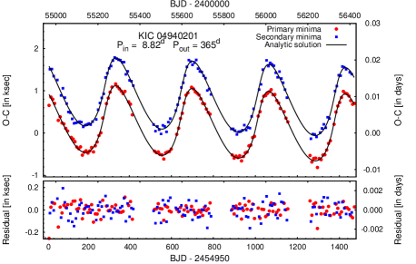
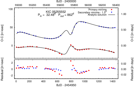
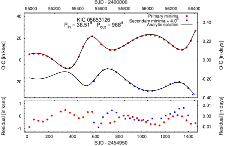
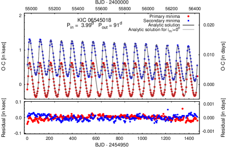
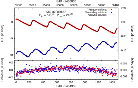
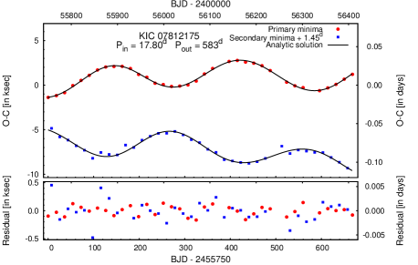
Figure 2: Eclipse Timing Variations (also known as $O-C$ curves) with fitted solutions for the first 6 of the 10 best-modeled systems (top) and the residual curves (bottom). Each panel contains the KIC number of the system, as well as the inner binary period and outer triple period. The points for the primary eclipses are shown in red, while the blue points are for the secondary eclipses. The fitted analytic solution is shown with the continuous black curves. (Note, we shifted the secondary curves toward the primaries, where it was necessary for a better visualisation; however, we strictly preserved the order (i.e., the sign of the displacement) of the two curves and, consequently, rigorously avoided introducing false intersections between the curves (an error made in some recent papers). Where there has been a shift, it is listed in the panel’s legend.)

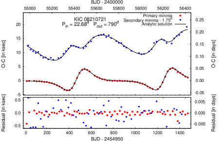
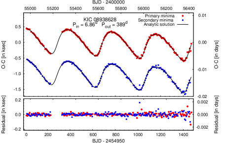
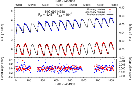
Figure 3: Eclipse Timing Variations with fitted solutions and residuals for the remaining 4 best-modeled systems. The specifications are otherwise the same as in Fig. 2.

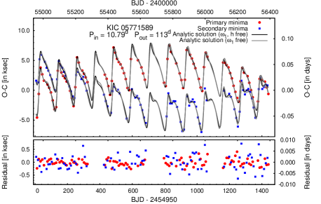
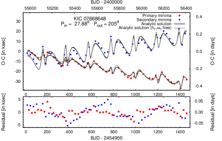
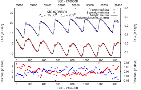
Figure 4: Eclipse Timing Variations with fitted solutions for the closest systems, i.e., those with the smallest ratios of $P_{2}/P_{1}$. The specifications are otherwise the same as in Fig. 2. (Note, where two solutions are given, the residual curve is shown only for the first one listed in the Tables.)

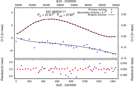
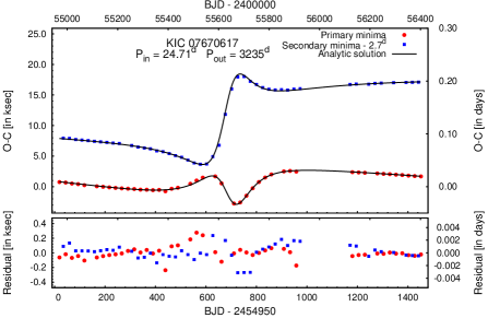
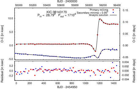
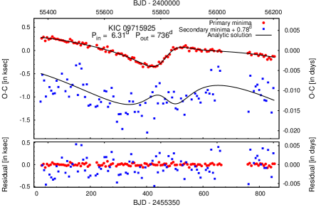
Figure 5: Eclipse Timing Variations with fitted solutions for the first 6 of our 12 systems with Kepler coverage that spans close to only one outer period or even less in some cases. The specifications are otherwise the same as in Fig. 2.

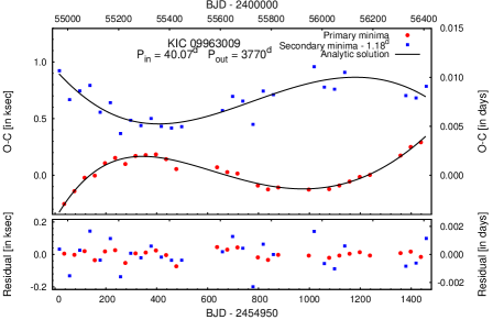
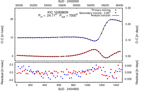
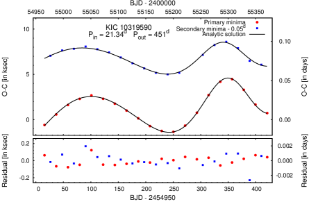
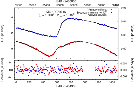
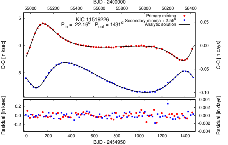
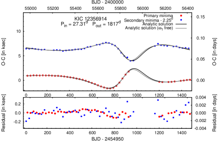
Figure 6: Eclipse Timing Variations with fitted solutions for the remaining 6 systems with Kepler coverage that spans close to only one outer period, or even less in some cases. The specifications are otherwise the same as in Fig. 2. (Note, where two solutions are given, the residual curve is shown only for the first labeled one.)

5 Results for the 26 Kepler Compact Hierarchical Triples

5.1 Overview of the Results

The ETV ($O-C$) curves for the collection of 10 CHTs with the most robustly fitting solutions are shown in Figs. 2, 3. As is the case for the other 16 systems, the fitted parameters as well as some additional interesting derived quantities are given in four tables. Table 3 contains the orbital elements for both orbits. Table 4, lists the 3D orbital orientations with respect to both the observational and the dynamical frames of references. Moreover, the ratio of the orbital angular momenta for the inner and outer binaries, $C_{1}/C_{2}$, is also given. In the most conservative hierarchical three-body approximation this value is considered to be small (or, asymptotically zero). Here, for retrograde systems, we somewhat arbitrarily use negative signs. Table 5 lists the constituent masses, mass ratios, LTTE-derived mass function and amplitudes of the separate constituents of the ETVs. It should be kept in mind that, in contrast to the ${\cal{A}}_{\mathrm{LTTE}}$ term, which gives the unique amplitude of the LTTE, the dynamical amplitudes may be, and are often strongly altered by the other orbital elements, as well as by the spatial configurations. Therefore, the latter are given only for a rough comparison. Finally, Table 6 lists different periods or timescales of the observable and dynamical apsidal motions and orbital precession, as well as other quantities which characterize the secular evolution of the systems. Most of the listed orbital elements are doubly averaged osculating orbital elements, which are calculated for the epoch $T_{0}$ which is given in the third column of Table 2. Exceptions are the angular variables ($\omega_{1}$, $g_{1}$, $h_{1}$, $i_{1}$, $i_{2}$) for which their values are given both for the moment of the first and the last observed eclipse. Realistic estimated parameter uncertainties are also listed in the tables. The uncertainties are given only for those variables that were included in either the LM fitting process or the grid search. The majority of the cited uncertainties come from either the covariance matrix of the LM-solution, or the step-size of the grid-search process; however, in a few cases we adopted more conservative errors, as will be discussed in the next section. For quantities fixed for all the runs, this is also noted on the same lines of the tables, and denoted by the letter ‘f’ after the numerical value. The 10 systems shown in Figs. 2 and 3 are listed above the first horizontal break line in these tables.

The next four systems listed in Tables 3-5 between the two horizontal break lines have their $O-C$ curves shown in Fig. 4. These are the systems for which the ratio of $P_{2}$ to $P_{1}$ is smallest among the systems we considered, and lies in the range of $7\lesssim P_{2}/P_{1}\lesssim 22$. This is to be compared with the range of $P_{2}/P_{1}$ of $\sim 16-57$ for the ten systems in Fig. 2. Our fits for these systems are significantly weaker, in our opinion, mainly due to insufficient modeling of the apsidal motion. In the case of three of these four systems we also give alternative solutions. A comparison of these solutions, however, reveals that despite the large uncertainties, our fits might yet be acceptable in the sense that the derived parameters can at least be used for statistical purposes (see Sect. 6).

Finally, in Figs. 5 and 6 we present the fitted ETVs for the dozen remaining systems. The fitted parameters for these are given in Tables 3-6 below the final horizontal break line. These systems also yield remarkably good fits to the analytic models, but they have outer periods, $P_{2}$, with only three exceptions, that are longer than 1000 days; half of the systems have $P_{2}$ longer than the Kepler mission. It is these longer periods that make the fits somewhat less reliable than for the systems shown in Figs. 2, 3. Nonetheless, the incomplete orbital coverage is somewhat compensated for by the fact that 3/4 of these systems have a clear periastron passage of the outer orbit during the course of the Kepler mission. Note, for one of these latter systems, an alternative solution is also given.

Table 3: Orbital Elements

KIC No.	$P_{1}$	$e_{1}$	$\omega_{1}$	$g_{1}$	$\tau_{1}$	$P_{2}$	$a_{2}$	$e_{2}$	$\omega_{2}$	$g_{2}$	$\tau_{2}$
	(day)		(deg)	(deg)	(MBJD)	(day)	(R⊙)		(deg)	(deg)	(MBJD)
04940201	8.8183	0.001(1)	194–202(16)	93–111	4965.42(38)	364.9(3)	278(24)	0.24(2)	247(5)	326	4864(7)
05255552	32.4787	0.307(1)	105–109(1)	311–322	4956.79(20)	862.2(2.9)	510(35)	0.43(1)	37(1)	62	4875(4)
05653126a	38.5071	0.272(010)	307–312(1)	220–231	4988.14(43)	968.4(1.4)	571(11)	0.19(1)	321(1)	53	5467(3)
06545018	3.9928	0.003(1)	180–225(1)	247–355	4964.84(1)	90.60(1)	122(2)	0.25(1)	226(1)	114	4970.2(3)
	3.9915	0.003(1)	179–228(1)	$-$	4964.83(1)	90.58(1)	119(1)	0.24(1)	229(1)	$-$	4970.4(1)
07289157	5.2674	0.083(1)	65–81(1)	215–249	4972.19(5)	243.4(1)	215(2)	0.31(1)	157(1)	127	4941.6(6)
07812175	17.7967	0.160(4)	326–328(2)	257–263	5004.63(8)	582.5(1.8)	367(50)	0.031(4)	213(6)	318	4790(11)
08023317	16.5778	0.251(1)	178–175(1)	82.3–82.0	4976.81(4)	610.6(5)	242(11)	0.25(1)	164(1)	249	5014(3)
08210721	22.6771	0.142(1)	156–159(1)	103–112	4964.93(10)	789.8(4)	498(11)	0.26(1)	211(1)	333	4628(4)
08938628	6.8630	0.003(1)	345–351(3)	51–67	4968.03(5)	388.5(3)	298(20)	0.20(1)	56(2)	304	4822(4)
09714358	6.4783	0.015(1)	142–379(1)	$-$	4965.11(1)	103.78(2)	116(5)	0.30(1)	120(2)	$-$	4977.4(6)
05771589	10.7866	0.013(1)	236–457(1)	134–398	4961.14(1)	113.14(1)	127(6)	0.23(1)	287(1)	7	4976.1(5)
	10.7866	0.013(1)	234–458(1)	174–583	4961.14(3)	112.97(3)	152(8)	0.13(1)	291(1)	50	4977.9(5)
06964043	10.7372	0.055(1)	77–115(1)	162–245	5195.10(1)	239.1(2)	248(14)	0.52(1)	311(2)	216	5110(2)
07668648	27.8764	0.065(5)	85–117(1)	$-32$–53	4976.75(8)	204.8(4)	192(11)	0.33(2)	352(4)	57	4918(3)
	27.8592	0.091(9)	88–108(1)	24–51	4976.97(6)	203.77(37)	204(11)	0.37(1)	341(4)	87	4922(3)
07955301	15.3633	0.031(1)	117–201(1)	182–341	4961.57(2)	209.43(14)	228(16)	0.28(1)	300(1)	189	4877.8(1.1)
	15.3714	0.029(1)	114–215(1)	37–152	4961.45(3)	209.06(10)	232(5)	0.32(1)	307(1)	47	4879.0(1.2)
04769799	21.9302	0.101(21)	330–331(21)	9–12	4971.59(1.14)	1231(8)	653(74)	0.19(1)	233(9)	95	5542(40)
05003117	37.6137	0.145(33)	308–309(9)	4–6	4989.04(80)	2150(100)	823(141)	0.26(1)	191(5)	75	4743(46)
05731312b	7.9461	0.420(1)	184(1)	255–256	4967.20(1)	906.7(3.4)	423(42)	0.58(1)	26(1)	282	4842(3)
07670617a	24.7050	0.246(5)	136–138(1)	53–57	4961.53(10)	3235(108)	1041(29)	0.70(1)	86(1)	167	5641(36)
08143170a	28.7868	0.146(3)	291–293(1)	160–163	4971.38(3)	1710(36)	864(19)	0.70(1)	109(1)	163	6121(27)
09715925	6.3082	0.201(8)	354(18)	278–279	5000.01(28)	736(36)	325(56)	0.38(2)	136(7)	232	5082(42)
09963009a	40.0714	0.224(102)	258–257(5)	258–257	4985.19(39)	3770(10)	1425(170)	0.24(6)	189(6)	9	4073(79)
10268809	24.7093	0.314(2)	143–145(1)	258–260	4965.57(3)	7000(1000)	2208(60)	0.74(1)	293(1)	227	6147(169)
10319590a	21.3370	0.026(1)	249–254(1)	155–162	4964.52(3)	451(3)	287(11)	0.17(1)	336(2)	67	4858(3)
10979716	10.6835	0.074(1)	106–108(1)	97–101	4962.31(6)	1045(4)	521(7)	0.44(1)	61(1)	231	4520(3)
11519226	22.1631	0.187(1)	359–360(1)	93–97	4977.11(4)	1431(1)	745(8)	0.33(1)	322(1)	236	5010(2)
12356914a	27.3080	0.403(30)	108(7)	251–252	4965.71(7)	1817(26)	948(36)	0.37(1)	10(1)	234	5876(18)
	27.3081	0.325(3)	113(1)	251–252	4966.04(4)	1811(26)	629(76)	0.39(1)	35(1)	346	5862(18)

Notes. (1) Single-valued columns represent doubly averaged osculating orbital elements for epoch $T_{0}$ (which is given in Table 2). (2) $\mathrm{MBJD}=\mathrm{BJD}-2\,450\,000$. (3) Double-valued columns give the corresponding orbital elements at the times of the first and the last eclipse observations. (4) Uncertainties in the last digits of the fitted parameters are given in parenthesis. (5) Blank spaces in the KIC-number column indicate an alternative solution for the same system denoted in the previous row.
${}^{a}:$ uniformly, and equally weighted primary and secondary eclipses; ${}^{b}:$ corrected secondary uncertainties (see text for details)

Table 4: 3D Orbital Orientations

KIC No.	$i_{\mathrm{m}}$	$i_{1}$	$i_{2}$	$n_{1}$	$n_{2}$	$\Delta\Omega$	$i_{0}$	$j_{1}$	$j_{2}$	$h_{1}$	$C_{1}/C_{2}$
	(deg)	(deg)	(deg)	(deg)	(deg)	(deg)	(deg)	(deg)	(deg)	(deg)
04940201	5.9(1.9)	85.0–85.9f	86.1–86.0	100.7	101(52)	$-5.9$	85.9	5.0	0.9	101.1–90.7	0.190
05255552	6.4(2.2)	83.7–84.1	89.5–89.4f	154.7	15(20)	$-2.7$	88.5	5.3	1.1	154.9–147.3	0.212
05653126	11.0(1.0)	87.0–88.1f	86.6–86.4	87.3	88(1)	$-11.0$	86.6	9.6	1.4	87.9–81.2	0.151
06545018	11.2(3)	86.0–77.2f	81.7–84.6	113.0	112(2)	10.4	82.7	8.5	2.8	292.3–228.6	0.326
	0.0f	88.0	88.0	$-$	$-$	0.0	88.0	0.0	0.0	$-$	0.321
07289157	4.3(1.3)	85.8–85.3	89.5–89.6f	30.1	30(10)	2.2	89.1	3.9	0.4	210.0–192.0	0.116
07812175	15.4(2.5)	85.9–86.7f	80.4–80.3	72.6	7(10)	$-14.9$	81.2	13.1	2.3	70.0–66.2	0.180
08023317	49.5(6)	88.0–89.4f	92.9–92.1	95.5	95.1(7)	$-49.3$	91.1	31.0	18.5	95.8–93.1	0.617
08210721	13.7(1.0)	89.5–90.5f	81.3–81.2	52.7	54(14)	$-11.0$	81.9	12.6	1.1	53.5–47.3	0.085
08938628	13.3(1.0)	87.0–85.0f	81.8–82.0	113.4	112(5)	12.3	82.2	12.2	1.1	344.8–350.8	0.091
09714358	0.0f	83.0f	83.0	$-$	$-$	0.0	83.0	0.0	0.0	$-$	0.455
05771589	21.9(4)	85.8–98.3f	90.0–86.5	100.0	101(4)	$-21.6$	89.1	17.2	4.7	101.4–57.6	0.280
	7.9(1.4)	85.9–78.7f	82.1–83.2	60.1	61(12)	$-6.9$	82.6	6.9	1.0	421.0–234.2	0.145
06964043	19.2(1.6)	91.2–79.2	89.5–91.6f	94.9	95(5)	19.1	89.7	16.4	2.7	275.0–229.2	0.169
07668648	40.9(1.5)	84.1–105.2f	102.5–85.2	117.3	115(2)	$-36.6$	94.5	22.5	18.4	117.6–60.7	0.825
	42.3(1.5)	83.9–86.3f	68.0–65.7	63.7	74(9)	$-40.6$	74.6	22.6	19.8	67.8–60.6	0.881
07955301	19.1(7)	83.0–63.6f	75.4–78.5	114.9	112(3)	17.9	76.4	16.5	2.6	292.1–216.2	0.161
	19.3(8)	83.1–87.1f	79.2–78.4	77.3	80(6)	$-19.2$	79.8	16.1	3.2	79.5–64.3	0.200
04769799	21.7(2.1)	86.0–85.7f	69.4–69.5	141.0	138(35)	14.4	72.1	18.1	3.6	318.8–317.1	0.204
05003117	44.0(1.0)	89.0–88.7f	66.3–66.3	124.1	115(9)	38.9	68.4	39.1	4.9	297.2–296.6	0.136
05731312	37.8(4)	88.5–88.0f	77.4–77.6	108.9	104(2)	36.4	79.8	28.3	9.5	286.1–285.0	0.347
07670617	147.1(5)	86.0–84.8f	89.3	82.4	98.6(9)	$-147.5$	88.6	142.9	4.3	98.5–100.4	$-0.124$
08143170	38.5(3)	89.0–89.6f	113.6–113.3	131.7	125.5(5)	$-30.5$	105.0	24.4	14.1	129.4–127.6	0.591
09715925	36.9(2.3)	83.2–83.6f	76.1	76.2	83(10)	$-36.9$	76.6	33.0	3.9	81.8–81.2	0.125
09963009	33.7(2.8)	89.0f	55.3	0.0	0(3)	$-0.0$	57.6	31.4	2.3	0.0–$-0.1$	0.077
10268809	23.7(4)	84.0–83.3f	93.8	66.1	65.7(1.3)	21.6	93.2	22.2	1.5	245.6–243.7	0.071
10319590	135.4(3)a	88.0–85.5f	94.0–94.4	93.7	88.8(8)	$-135.4$	94.1	128.5	6.9	89.3–92.5	$-0.154$
10979716	9.0(1.3)	86.0–86.0f	77.2–77.2	9.5	9.7(9.3)	$-1.5$	78.0	8.1	0.9	9.7–7.9	0.110
11519226	17.0(3)	88.0–87.2f	89.3–89.4	85.7	85(1)	17.0	89.2	15.6	1.4	265.4–262.5	0.091
12356914	143.1(1.0)	88.0–88.5f	120.4–120.3	37.2	135.6(6)	155.1	126.8	133.9	9.2	311.1–312.2	$-0.223$
	40.2(3)	88.0–87.5f	116.7–116.8	42.5	49.0(5)	29.2	111.0	31.7	8.5	226.3–225.0	0.281

$a$: numerical checks have also resulted in prograde solutions with $i_{\mathrm{m}}=43\pm 2\degr$

Table 5: Mass related and other quantities

KIC No.	$f(m_{\mathrm{C}})$	$m_{\mathrm{C}}/m_{\mathrm{ABC}}$	$q_{1}$	$m_{\mathrm{AB}}$	$m_{\mathrm{C}}$	${\cal{A}}_{\mathrm{LTTE}}$	${\cal{A}}_{\mathrm{L1}}$	${\cal{A}}_{\mathrm{L2}}$	${\cal{A}}_{\mathrm{S}}$
	(M⊙)			(M⊙)	(M⊙)	(ksec)	(ksec)	(ksec)	(ksec)
04940201	0.062	0.307(90)	0.90f	1.50(62)	0.66(26)	0.196	1.845	0.008	0.049
05255552	0.061	0.294(10)	0.50(5)	1.69(72)	0.71(36)	0.327	12.679	0.521	0.653
05653126	0.098	0.334(20)	0.37(10)	1.77(17)	0.89(7)	0.436	13.935	0.677	0.587
06545018	0.036	0.232(10)	0.80(1)	2.29(13)	0.69(5)	0.064	1.161	0.016	0.057
	0.036	0.235(10)	0.84(1)	2.11(11)	0.65(4)	0.064	1.167	0.012	0.056
07289157	0.139	0.395(10)	0.48(1)	1.37(9)	0.89(4)	0.189	1.348	0.034	0.034
07812175	0.050	0.327(15)	0.85(1)	1.02(74)	0.49(31)	0.252	4.585	0.032	0.140
08023317	0.002	0.103(30)	0.53(1)	1.29(15)	0.15(5)	0.079	1.311	0.037	0.039
08210721	0.097	0.335(20)	0.16(1)	1.77(20)	0.89(8)	0.373	6.252	0.397	0.199
08938628	0.244	0.474(70)	0.91(1)	1.25(54)	1.12(28)	0.323	1.571	0.004	0.029
09714358	0.010	0.172(50)	0.45(1)	1.65(29)	0.34(10)	0.046	2.068	0.127	0.149
05771589	0.067	0.314(50)	1.45(5)	1.48(33)	0.68(14)	0.093	8.962	$-0.319$	0.923
	0.443	0.497(60)	1.20(10)	1.88(71)	1.85(37)	0.173	13.410	$-0.205$	1.307
06964043	0.271	0.424(10)	0.85(5)	2.06(6)	1.51(6)	0.229	8.488	0.099	0.614
07668648	0.006	0.144(60)	0.69(1)	1.96(42)	0.33(14)	0.059	16.730	0.867	2.714
	0.005	0.132(50)	0.58(1)	2.38(46)	0.36(16)	0.054	16.082	1.249	2.726
07955301	0.306	0.453(70)	0.97(1)	1.99(85)	1.65(42)	0.230	14.869	0.014	1.235
	0.224	0.393(20)	0.85(5)	1.27(29)	1.53(13)	0.205	13.374	0.179	1.151
04769799	0.036	0.262(110)	0.80f	1.83(92)	0.65(36)	0.369	2.786	0.020	0.052
05003117	0.045	0.332(170)	0.50(10)	1.08(62)	0.53(40)	0.562	6.233	0.131	0.121
05731312	0.001	0.109(100)	0.30(1)	1.10(39)	0.13(13)	0.089	0.365	0.012	0.006
07670617	0.085	0.389(30)	0.90f	0.89(17)	0.56(8)	0.939	5.238	0.018	0.111
08143170	0.005	0.126(20)	0.55(5)	2.59(24)	0.37(7)	0.226	4.401	0.159	0.207
09715925	0.007	0.206(170)	0.20f	0.68(48)	0.18(17)	0.145	0.361	0.011	0.004
09963009	0.104	0.410(10)	0.40(10)	1.61(32)	1.12(28)	1.083	4.918	0.091	0.057
10268809	0.317	0.477(30)	0.70f	1.55(97)	1.41(43)	2.238	3.470	0.025	0.040
10319590	0.098	0.398(40)	0.60(5)	0.94(20)	0.62(9)	0.262	10.790	0.306	0.532
10979716	0.098	0.394(10)	0.96(1)	1.05(8)	0.69(3)	0.453	1.533	0.002	0.022
11519226	0.267	0.463(10)	1.23(1)	1.44(9)	1.25(5)	0.773	4.867	$-0.028$	0.089
12356914	0.020	0.208(40)	0.50(10)	2.75(44)	0.72(16)	0.368	2.741	0.060	0.051
	0.005	0.190(120)	0.70(1)	0.83(40)	0.19(14)	0.235	2.575	0.030	0.050

Table 6: Secular evolution related quantities

KIC No.	$P_{\omega_{1}}$	$P_{h}$	$P_{g_{1}}^{\mathrm{inst}}$	$P_{g_{1}}^{\mathrm{mod}}$	$\varepsilon$	$P_{GR+tide}/P_{3b}$
	(years)	(years)	(years)	(years)
04940201	171.7	138.8	76.9	75.9	0.01	608
05255552	238.7	123.7	81.2	90.0	$-0.12$	4472
05653126	272.1	199.2	115.9	115.0	$-0.06$	4295
06545018	33.2	23.0	13.6	13.2	0.04	234
	29.2	22.1	12.6	12.6	0.00	300
07289157	90.6	79.8	42.4	42.3	0.00	387
07812175	284.2	170.2	108.6	104.3	0.05	1925
08023317	$-595.3$	588.2	$-4558.5$	1051.2a	1.20	33
08210721	344.3	235.8	142.1	136.7	0.04	1523
08938628	178.2	150.7	82.9	81.8	0.07	408
09714358	30.6	21.0	12.5	12.5	0.00	1731
05771589	6.5b	32.4b	6.6	6.8	0.18	10456
	6.5c	7.5	4.0	4.1	0.02	14243
06964043	27.0	26.0	13.5	15.2	0.14	3810
07668648	41.6	24.7	16.1	27.9	0.68	18146
	62.9d	193.2d	14.4	31.0	0.72	17554
07955301	18.1	18.7	9.5	10.9	0.14	10942
	14.7e	96.7e	11.4	11.9	0.14	7979
04769799	814.5	818.8	423.0	494.0	0.18	548
05003117	835.6	1556.1	591.2	1707.5	1.27	1196
05731312	$-5613.1$	1005.3	1441.6	1165.3	0.25	25
07670617	926.8f	$-1623.7$	1382.2	1367.1	0.51	278
08143170	929.0	890.3	475.1	847.8	0.59	524
09715925	$-3182.2$	1163.4	2545.3	1270.0	0.63	18
09963009	$-19194.3$	2672.4	3789.5	2426.2	0.48	154
10268809	1830.4g	3333.5	2799.2	2600.1	0.08	90
10319590	79.4	$-131.2$	57.7	80.8	1.86	5322
10979716	750.6	611.1	340.5	333.3	0.02	256
11519226	954.8	510.3	340.6	319.9	0.06	693
12356914	$-8378.2$	$-1499.5$	3036.1	2019.1	0.59	60
	$-10311.8^{h}$	1335.8	2455.9	1653.6	0.57	184

Notes. (1) For the definition and a detailed discussion of the quantities listed in the Table see Appendix  C. (2) A negative sign in the apsidal motion periods $P_{g_{1}}$ and $P_{\omega_{1}}$ indicates retrograde apsidal motion. (3) A negative orbital precession period $P_{h}$ denotes prograde orbital precession, i.e., nodal progression.
$a$: dynamical apse librates; $b$: unconstrained apsidal motion and nodal regression (constrained values are $P_{\omega_{1}}=15.6$ y, and $P_{h}=10.9$ y, respectively); $c$: unconstrained apsidal motion (theoretical $P_{\omega_{1}}=8.3$ y); $d$: unconstrained apsidal motion and nodal regression (constrained values are $P_{\omega_{1}}=29.6$ y, and $P_{h}=25.5$ y, respectively); $e$: unconstrained apsidal motion and nodal regression (constrained values are $P_{\omega_{1}}=24.8$ y, and $P_{h}=20.1$ y, respectively); $f$: unconstrained apsidal motion (constrained $P_{\omega_{1}}=4366.1$ y); $g$: unconstrained apsidal motion (constrained $P_{\omega_{1}}=13392.6$ y); $h$: unconstrained apsidal motion (constrained $P_{\omega_{1}}=-4168.7$ y)

5.2 Robustness of System Parameter Determinations

The amplitudes or, more strictly, the magnitude of the amplitudes, of the different contributors to the ETV curves (tabulated in columns 7–10 of Table 5) reveal that in our entire sample, the quadrupole-level dynamical perturbations clearly dominate the ETV on the time-scale of the outer orbital period.

A review of the parameter uncertainties, listed in Tables 3–5, reveals that the most robustly determined parameters are the eccentricities, $e_{1,2}$; arguments of periastron in the observational frame, $\omega_{1,2}$; the times of periastron passage of the outer orbit, $\tau_{2}$; and naturally, for fully covered outer orbits, the outer orbital period, $P_{2}$. In the case of $e_{1}$ and $\omega_{1}$ the high accuracy and robustness arises mainly from the precisely measured displacement of the secondary eclipses from a phase of $\phi=0.5$, which leads directly to a very high accuracy determination of the quantity $e_{1}\cos\omega_{1}$. Then, when at least one or two full outer orbital periods are observed, the shape of the ETV curve breaks the $e_{1}$–$\omega_{1}$ degeneracy, which results in a typical-LM uncertainty of $\delta\omega_{1}\sim 0.1\degr$ which implies an uncertainty in $\delta e_{1}$ of $\sim 10^{-4}$. A good example from our sample is KIC 04940201 (see left upper panel of Fig. 2) which demonstrates clearly that an inner binary eccentricity of $e_{1}\simeq 0.001$ results in a clearly distinguishable and measurable displacement of the secondary eclipse curve. Despite this, however, we decided to adopt the somewhat more conservative uncertainty limits of $\delta e_{1}\geq 0.001$ and $\delta\omega_{1}\geq 1\degr$ for these two orbital parameters. One reason is, of course, the possibly of systematic effects which will certainly arise from the approximate nature of our analytic model. The other reason has to do with the perturbed and, therefore, continuously varying nature of these elements. As will be illustrated in Appendix E the amplitudes of these perturbations may exceed even these more conservative error limits over a timescale of days. Furthermore, in accord with our numerical tests in Appendix E we also introduce another conservative error limit for the outer eccentricity by fixing $\delta e_{2}\geq 0.01$.

An additional important parameter is the mutual inclination, $i_{\mathrm{m}}$. As will be discussed in the Statistical Results section (Sect. 6), this parameter exhibits a bimodal distribution. Here we concentrate only on the characteristics of the uncertainties in different regimes of $i_{\mathrm{m}}$. The LM-uncertainties in this quantity are generally around $1-2\degr$. On the other hand, from the additional numerical runs that we made, we find significantly larger uncertainties for low mutual inclination systems than for systems with higher mutual inclinations (i.e. $i_{\mathrm{m}}>30\degr$). This should result from the fact that, for nearly coplanar configurations, the $i_{\mathrm{m}}$-dependence is much shallower than for higher mutual inclinations. Moreover, note that in this regime the short-term and octupole perturbations have a relatively higher weight, in contrast to the quadrupole terms. This was our main reason for introducing these latter terms, and in this way we were actually able to reduce the uncertainties in $i_{\mathrm{m}}$ in this regime. (They had been even larger before.) In conclusion, we can say that, even in spite of the somewhat larger uncertainties in $i_{\mathrm{m}}$ for the near-coplanar situations, the accuracy that was obtained is evidently sufficient to be able to make statistically meaningful statements concerning the mutual inclination distribution of our sample.

Considering the other parameters that describe the complete spatial configuration of the systems, the node-like angle, $n_{2}$, was adjusted either with the Levenberg-Marquardt fitting procedure, or with a grid-search, while its inner orbit counterpart, $n_{1}$, was constrained in a geometrical way from the corresponding spherical triangle, as is discussed in Appendix D. The estimated uncertainties for this parameter cover a substantially wider range than that for the other parameters mentioned above. Note also, that for some triples, this parameter was controlled subjectively to exclude solutions which would have resulted in inclination angle variations that were too rapid, or opposite in direction to those which were observed. The larger uncertainties may arise primarily from the fact that these parameters, in most cases, appear in linear combinations: $\alpha=n_{2}-n_{1}$, $\beta=n_{1}+n_{2}$, where $\alpha$ and $\beta$ are typically not determined with the same accuracy. (For the prograde case, $\alpha$ is much more constrained than $\beta$, while for a retrograde configuration, the reverse is true.) Therefore, their individual values remain somewhat undetermined.

Consider, finally, the mass-related parameters, which are the most important—at least from an astrophysical point of view. Unfortunately, here the picture is not so sanguine. As was expected, the mass ratio of the outer orbit, being relatively well determined, was found to have an uncertainty of a few to ten percent in most systems. The mass ratio of the inner binary appears only in the octupole terms. Due to the smaller-amplitude contribution of these terms, we did not expect highly robust results for this parameter. Qualitatively, however, in most cases our solutions have led to physically reliable values, seemingly in accord with the crude preliminary estimates deduced from the flux ratios of the primary and secondary eclipses. Nevertheless, on the other hand, considerable caution is required, since in some cases we arrived at implausibly small or large numerical values; this could be a consequence of the physical model which might be insufficient in some extreme situations, as will be discussed in the context of KIC 07670617 in Appendix E. Although, a combination of the dynamical effects and the LTTE, in principle, should lead to physical mass determinations for the system components, our results, unfortunately, show some of the largest uncertainties in these quantities. This is, however, not so surprising. In the systems we investigated, the LTTE provides only a minor contribution to the ETV pattern. The one exception is KIC 10268809 where the amplitude ratio was found to be ${\cal{A}}_{\mathrm{L1}}/{\cal{A}}_{\mathrm{LTTE}}\sim 0.64$. We carried out some tests with that solution to check whether we were able to recover the individual masses in such a case (see Appendix E). We found that, unfortunately, even if the relevant parameters, $a_{\mathrm{AB}}\sin{i_{2}}$ and $m_{\mathrm{C}}/m_{\mathrm{ABC}}$, are obtained with a few percent accuracy, the uncertainty obtained for the individual masses becomes as high as a 10%-20%. While this level of accuracy may be insufficient for some astrophysical considerations; it should be acceptable for statistical purposes as well as for initial estimates used in future follow-up studies.

5.3 General Properties of the CHTs

The ETV curves of our 26 systems show significant diversity. In the simplest cases, both the primary and secondary ETV curves look similar to one another and are purely ‘monoperiodic’ (i.e., have only one maximum per outer period; KICs 04940201, 0654508, 08938628). However, there is a nearly continuous transition from this type of system to much more complex situations. These include cases where the two curves are still predominantly monoperiodic, but an extra hump begins to appear in one or both ETV curves and, in a parallel way, the primary and secondary ETV curves become more and more distinct from each other (e.g., KICs 07289157, 10979716, 09714358, 07955301, 05771589, 06964043). Then there are the most peculiar ones, having a ‘double periodicity’ (two distinct maxima per outer period), and/or anti-phased primary and secondary ETV minima. Finally, there are ETV curves that are almost flat, but with a simple jump (which typically have remarkably different amplitudes in the primary and secondary ETV curves).

As discussed in Borkovits et al. (2011) these features are mostly governed in a complex way by the eccentricities on the one hand, and the spatial orientations of the orbits with respect to each other and to the observer, on the other hand, while the mass and period ratios only scale the ETV curves in amplitude and time, respectively. We emphasize again that here we primarily refer to the $P_{2}$ time-scale quadrupole perturbation term, which, however dominates the ETVs in all of the 26 systems. Due to this complexity, we need considerable caution in making any qualitative assessment of a system’s orbital properties from only the morphology of its ETV curve. For example, it can be said that a triple with small mutual inclination and negligible inner eccentricity always produces a monoperiodic ETV but the reverse statement would already be false, as was illustrated in Fig. 5l of Borkovits et al. (2011), which also shows monoperiodic ETVs for a perpendicular configuration.

Some statements about the systems’ general characteristics, however, can be made from a perusal of the overall qualitative structure of the ETV curves. Thus, if during the most rapidly varying portion of the ETVs, i.e., around periastron passage of the wide orbit, the net variation is positive, i.e., the system clock becomes more delayed (as is the case in all of the systems that we investigated), we can exclude a near-perpendicular configuration in any of our investigated systems. (The analytical verification of this is given in Appendix A.) In such a case, a double periodicity suggests significant mutual orbital inclinations, but, simultaneously, only moderate or small eccentricities. (As for a high-eccentricity case, the period “doubling” would reduce to a “spike” in the ETV curve.) Another, natural conclusion, is that the steeper a short section of the ETV curve is, the higher one or both of the eccentricities are.

Considering the apsidal motion contribution to the ETVs, the situation is simpler. If the secondary (blue) ETV curve is located below the primary (red) ETV curve, it indicates that the secondary eclipses are “in a hurry” with respect to the primary’s (i.e., the secondary eclipses occur before orbital phase 0.5). Consequently, in these cases the periastron passage of the inner binary orbit occurs between the primary and secondary eclipses (i.e., in the range of $-90\degr<\omega_{1}<90\degr$). Since the maximum separation between the primary and secondary ETV curves occur when $\omega_{1}=0\degr$ (secondary ETV curve is below), or $\omega_{1}=180\degr$ (secondary ETV curve is above), the divergence or convergence of the two curves provides some initial information on the location of $\omega_{1}$ in the various quadrants, as well. These preliminary assessments not only provide us with general insights into the relations among, and values of, the system properties and ETV curve morphologies, but they may also help in finding reliable initial parameters for the LM-fitting processes. A detailed discussion is given in Appendix E.

Figure 7: The Kepler light curve of KIC 04769799 (red) exhibits characteristic, uneven eclipse depth variations. The black line represents the rescaled and mirrored value of $\sin{i_{1}}$, calculated from our ETV solution. The similiraty between the two nicely illustrates that the eclipse depth variations can be attributed to the net effect of secular nodal regression and the $P_{2}$-period perturbations of the dynamical node. Note again, that none of the lightcurve characteristics (including eclipse depth variations) are directly built into our analytic model and, therefore, do not constrain our ETV solution.

5.4 Notes on individual systems

5.4.1 Group I systems

KIC 04940201. This system has the lowest inner-binary eccentricity of our sample. The absence of eclipse depth variations suggests that the inferred mutual inclination angle of $i_{\mathrm{m}}=5.9\degr\pm 1.9\degr$ may be a bit overestimated. (The possible reasons were discussed earlier in Sect. 5.2.) This system was included in the early Kepler-field low-mass eclipsing binary study of Coughlin et al. (2011).

KIC 05255552. A rather unique, triply-eclipsing system, with one of the largest amplitude ETV curves. Amongst the recently discovered triply eclipsing systems it has the longest outer orbital period ($P_{2}=862\pm 3$ days). Moreover, both orbits are remarkably eccentric, i.e., $e_{1}=0.307\pm 0.001$ which is among the largest in our sample, and $e_{2}=0.43\pm 0.01$. This CHT is also quite compact $P_{2}/P_{1}\sim 27$. Unfortunately, Kepler observations ended right during the third set of outer eclipsing events, and the only outer periastron passage in the Kepler-era occurred during a gap in the data.

KIC 05653126. This system exhibits remarkably high amplitude, rapid eclipse depth variations which are in good correspondence with the inferred system geometry parameters. Secondary eclipses occur only a few months after the outer periastron passage. For this system we used constant and equal uncertainties for both the primary and secondary ETV points, instead of individual uncertainties, because the use of the latter clearly overweights the primary curve with respect to the secondary one.

KIC 06545018. This system has the shortest inner period ($P_{1}=3.99$ days) as well as outer period ($P_{2}=90.6$ days) of all the systems in our sample. We give two solutions. In the first, $i_{\mathrm{m}}$, as usual, was allowed to vary freely. The result is $i_{\mathrm{m}}=11.2\degr\pm 0.3\degr$ which clearly contradicts the lack of eclipse depth variations. Therefore, we give an alternative, coplanar (i.e, $i_{\mathrm{m}}\equiv 0\degr$) solution. Note, despite the fact that the out-of-eclipse light curve clearly reveals tidally-induced ellipsoidal effects, the apsidal motion even here is also clearly dominated by dynamical effects, similar to the other systems we have investigated.

KIC 07289157. Another exemplary triply eclipsing system. A detailed description of its analysis is given in Appendix E. The residuals of our solution show a clearly parabolic trend. Therefore, we carried out an additional fitting run, including a second-order polynomial together with all the other parameters adjusted previously. This second fit resulted in a substantially lower $\chi^{2}$ value (half of the previous one), but all of the previously adjusted parameter values were preserved to within the standard errors of the first solution. From this combined parabolic and third-body solution we obtained a (constant) rate of period change of $\Delta P_{1}=-9.3\pm 0.3\times 10^{-8}$ day/cycle. This inferred period decrease might be a slight indicator of either an additional, more distant component in the system, or some orbital shrinking of the binary; however, we cannot exclude the possibility that it is a pure consequence of the imperfect modeling of the secular third-body perturbations.

KIC 07812175. This system is located nearly midway between two substantially brighter KIC objects (07812167 and 07812179) that are separated by about 15^′′. This is likely the cause of some spurious eclipse depth variations in this system during alternating Kepler quarters. However, this does not materially affect our ETV analysis. It has the lowest outer eccentricity among our collection of triples ($e_{2}=0.031\pm 0.004$).

KIC 08023317. The highest mutual inclination triple ($i_{\mathrm{m}}=49.5\pm 0.6\degr$) in the sample. It also holds claim to the lowest outer mass ratio of $m_{\mathrm{C}}/m_{\mathrm{ABC}}=0.103\pm 0.03$ or, $q_{2}\sim 0.11$. As a consequence, in contrast to the majority of hierarchical systems, the orbital angular momentum is predominantly stored in the inner orbit. The $C_{1}/C_{2}=0.617$ ratio is also one of the highest amongst our 26 systems. We have chosen this unusual system to illustrate the operation of our analysis in the medium mutual inclination regime, and further details can be found in Appendix E.

KIC 08210721. Another totally eclipsing binary system with primary transits and very shallow secondary occultations. Our solution indicates a rapid variation in inclination ($\Delta i_{1}\sim 1\degr$); however, the totality of the eclipses might explain the absence of the eclipse depth variations. On the other hand, a more detailed inspection reveals that the eclipse durations also remain unchanged; therefore, the mutual inclination angle that we obtained is probably overestimated a bit.

KIC 08938628. The inner binary shows rapidly decreasing eclipse depths, which is in accord with our solution.

KIC 09714358. One of the four CHTs in the sample with a period ratio $P_{2}/P_{1}<20$. Because of the lack of eclipse depth variations, we searched only for co-planar solutions. Despite the small period ratio, we found the solution we obtained to be reliable enough to rank this CHT in the first group of our systems. Note that the out-of-eclipse light curve reveals other stellar variability, as was reported also by Debosscher et al. (2011).

5.4.2 Group II systems

KIC 05771589. Shallow eclipses with first decreasing, and then increasing, depths. The out-of-eclipse light curve sections are also distorted. We give two alternative solutions for this system. In the first, both the nodal regression and apsidal motion rates are unconstrained, while in the second case, nodal regression was constrained. The fit is quite poor in both cases, and neither of them is in accord with the characteristics of the eclipse depth variations. The orbital elements, however, with the exception of the outer eccentricity, are similar in the two solutions. In this triple, as in the other three systems, which were categorized into group II, a more sophisticated modeling is necessary.

KIC 06964043. Triply eclipsing system with shallow inner eclipses, and substantially deeper outer ones with variegated structures. The (inner) eclipse depth variation is opposite to that of the previously discussed system, i.e., an interval of increasing eclipse depths is followed by one with decreasing depths. For this system we were able to find a constrained solution (both in the apsidal advance and nodal regression); however, its reliability is similarly questionable, as in the previous case.

KIC 07668648. The light curve reveals continuously increasing eclipse depths, and even the primary and secondary eclipses are interchanged after a few cycles. A few additional shallow eclipses, not due to the binary, are also observed. Since these occurrences match the outer companion’s period and phase, we can conclude that this is not a blending of two systems in the Kepler photometric aperture for this object, but rather KIC 07668648 is also a marginally triply eclipsing system. It is also has the lowest period ratio ($P_{2}/P_{1}<7.3$), not only in our sample, but amongst all the known triple systems which contain an eclipsing inner binary. Accordingly, both of our fits (with constrained and unconstrained secular effects) are quite poor and, therefore, this triple system also requires an improved analysis.

KIC 07955301. This system exhibited rapid and remarkable eclipse depth growth during the first two years of the Kepler observations. Furthermore, similarly to the previous triple, the depths of the two kinds of eclipses also interchanged after the first few eclipses. (For this reason, in this most recent analysis we also interchanged the two kinds of eclipses. Therefore, the eclipse timings which were analyzed in Rappaport et al. 2013 as primary eclipses, are now considered to be secondary eclipses.) This system was also analysed by Gaulme et al. (2013) who found that the light curve shows clear red giant pulsations, from which they concluded that the tertiary should be a red giant with $M_{3}=1.2\pm 0.1\,M_{\odot}$, and $R_{3}=5.9\pm 0.2\,R_{\odot}$. The presence of such a luminous tertiary explains the shallow binary eclipses, as well. We present two solutions, first with constrained apsidal motion and orbital precession, and the second, without.

5.4.3 Group III systems

KIC 04769799. The very shallow secondary eclipses disappear completely before the periastron passage of the outer system. The amplitude of the primary eclipses also nicely exhibits the inclination jump on the $P_{2}$-timescale, with a net secular decrease. Our fit seems to be quite reliable, even in the sense of reproducing the light curve features (see Fig. 7); however, because of the absence of the information afforded by the secondary eclipses during a substantial portion of the Kepler observations, we classified this doubly low-eccentricity triple with the group of uncertain cases.

KIC 05003117. Slightly decreasing eclipse depths, and shallow secondary eclipses. The outer period is found to be substantially longer than the observed time-span of the Kepler observations.

KIC 05731312. Despite its relatively short inner period ($P_{1}\simeq 7.95$ days), this binary has the largest inner eccentricity ($e_{1}=0.420\pm 0.001$). The outer eccentricity is also amongst the highest ($e_{2}=0.58\pm 0.01$). As a consequence, the ETV shows a marked spike during the outer periastron passage. The amplitude of the ETV, however, is low (less than 0.01 days even for the higher amplitude secondary ETV curve). That is a consequence of the relatively wide separation of the triple ($P_{2}/P_{1}=114.1$, which is one of the highest in the sample) on the one hand, and the low mass of the ternary component ($m_{\mathrm{C}}/m_{\mathrm{ABC}}=0.11\pm 0.01$ is the second smallest ratio) on the other hand. In theory, more than one and a half outer cycles are covered but, unfortunately, only one periastron passage is located very near the middle of the Kepler measurements, and with the exception of this $\sim 400$-day-long interval, the ETV is almost featureless before and after, during the remaining 1000 days. Despite this, our solution seems to be reasonable (including the reconstruction of the jump-like eclipse depth decrease near the periastron passage). Note, this is another system where the use of the individual ETV point uncertainties resulted in an overweighted primary ETV curve and, therefore, the secondary ETV curve was not well fit. This is especially the case for the final Kepler quarters when, after periastron passage, the eclipse depths decreased significantly. As a compromise, we somewhat arbitrarily reduced the uncertainties in the secondary points by a factor of three.

KIC 07670617. This system shows a marked periastron passage with a sharp step-like feature in the ETV of the secondary, which is clearly also reflected in the light curve (see Fig. 22, in Appendix E). The outer binary is one of our three highest eccentricity systems ($e_{2}=0.70\pm 0.01$). The reliability of our retrograde solution is discussed in Appendix E. For this system we also preferred the use of constant and equal uncertainties in the ETV points.

KIC 08143170. The ETV curves, at first sight, show remarkable similarities to the previously discussed system. The inner binary light curve, however, in the present case exhibits only a minor, almost unnoticeable eclipse depth variation (increase) around periastron passage. The former property (i.e., the similarity of the ETV curve segments) can be explained by the similarly high outer eccentricities ($e_{2}=0.70\pm 0.01$), and also with their similar mutual inclinations (this is in spite of the fact that this system has a prograde outer orbital configuration, in contrast to the retrograde outer orbit of KIC 07670617). On the other hand the minor eclipse depth variations here might be explained by the totally eclipsing nature of KIC 08143170, in which case the eclipse depths are less sensitive to small variations in the inclination. This is especially true for occultations where the inclination affects only the eclipse duration. This is another triple for which the equal, global ETV uncertainties mode was used.

KIC 09715925. The light curve exhibits a step-like, moderate eclipse depth growth during the periastron passage. The very shallow and short secondary eclipses (which in most cases contain only 3–4 Kepler long cadence points) makes our solution less reliable. However, despite the large uncertainty in the outer period, most of the orbital elements, and the mutual inclination also seem to be reliable, at least qualitatively.

KIC 09963009. This system has the longest period inner binary ($P_{1}\simeq 40.1$ days) in our sample. Our solution points to one of the longest outer periods ($P_{2}\sim 3770$ days) which suggests a wide, weakly interacting system ($P_{2}/P_{1}\sim 94$). The relatively short coverage of the outer orbit, the low ETV amplitude, and the lack of marked features in the ETV curves make our solution somewhat untrustworthy. On the other hand, this triple allows us to illustrate the worthiness of including additional available information into the solution process. For this system we found two strongly different solutions with similar $\chi^{2}$ values; however, taking into consideration some of the lightcurve properties, we were able to eliminate one of these alternative solutions. This was because the Kepler light curve exhibited constant primary eclipse depths, but decreasing secondary depths, from which we concluded that the inner orbit’s periastron passage should be located closer to the primary than the secondary eclipse. Therefore we rejected the solution which resulted in $\omega_{1}=106\pm 10\degr$, and retained the one with $\omega_{1}=258\pm 5\degr$. (Here, again, we utilized the global and equal ETV uncertainty mode.)

KIC 10268809. Opposite to the case of the previous triple, these primary eclipses exhibit marked depth variations (similar to those shown in Fig. 7), while the secondary eclipses exhibit only minor decreases in depth. The amplitudes of the two kinds of eclipses also interchange around BJD 2 455 800. Our finding of $\omega_{1}=143\pm 1\degr$ is in accord with this fact but, for the very long inferred outer period ($P_{2}=7\,000$ days), some caution is needed concerning the reliability of these results. Note, this is the only triple where the LTTE amplitude is comparable to the quadrupole dynamical term. Therefore, we use our solution in Appendix E to test whether the individual stellar masses can be recovered in such circumstances.

KIC 10319590. As was already reported in Rappaport et al. (2013), the eclipses completely disappeared after the first 400 days of the Kepler observations. Previously SS Lac (Zakirov & Azimov, 1990) and V907 Sco (Lacy et al., 1999) were the only two EBs where the same phenomenon was documented. Our solution resulted in an outer orbit with a period, $P_{2}=451\pm 3$ days, that is very close to the observational window where the eclipses were present. The double periodicity in the ETV curves, however, is clearly seen and therefore we believe that this finding for $P_{2}$ is reliable. Our original solution revealed a retrograde orbit with $i_{\mathrm{m}}=135.4\pm 0.3\degr$, but our numerical tests have shown that it cannot be distinguished significantly from the corresponding prograde solutions. An indirect verification of our solution (independent of its prograde or retrograde nature) comes from the fact that the node-like parameter $n_{1}$ was found to be around $90\degr$. This provides the fastest instantaneous precession rate during the entire nodal period (see Eq. [119]) and, therefore, produces $\Delta i_{1}=-2.5\degr$ inclination variation during only 1.1 year of a $\sim 131$-year-long precession-cycle, in good correspondence with the relatively rapid disappearance of the eclipses. (Because of the rapid eclipse depth variations, we utilized equal global uncertainties for the ETV points in order to avoid underweighting those points derived from the last, just-disappearing, very shallow, grazing eclipses.)

KIC 10979716. The ETV curves for this system, and also the resultant fitted parameters, resemble in most aspects those of KIC 07289157. The main exception is in the lack of eclipse depth variation, which is well explained by the fact that the two orbits intersect each other close to the celestial plane $h_{1}=9.7\degr-7.9\degr$, in which case the observable precession rate becomes practically zero. This system was placed in the third group only because of the absence a second outer periastron passage; however, our solution should have almost the same robustness as for the group I systems.

KIC 11519226. Besides KIC 05771589, this is the only system, where a mass ratio of $q_{1}>1$ was found. Since there is only a minor difference in depths between the two eclipses in the binary, the $q_{1}=1.23\pm 0.01$ value might even be correct. Our solution has also reveals that the binary line of the apsides lies almost perfectly in the celestial plane ($\omega_{1}\sim 359\degr\pm 1\degr$). The durations of the two eclipses are similar which is also in accord with this result. The weakness of our fit is, however, that our solution would predict an inclination angle variation of nearly $\Delta i_{1}\sim-0.8\degr$ during the Kepler prime mission, but the light curve, despite the partial eclipses, does not show eclipse depth variations.

KIC 12356914. The light curve exhibits deep primary eclipses and significantly shallower, flat-bottomed secondary eclipses that are longer in duration. There are no eclipse depth variations. We give two alternative solutions. The constrained apsidal motion fit resulted in a retrograde solution, while the unconstrained fit yielded a prograde solution. The main weakness of both solutions is that they put the inner periastron passage close to the secondary eclipse which seems to contradict the fact that the secondary event is substantially longer, (i.e., occurs when the inner binary components are moving the slowest). Therefore, the reliability of these results could be questionable. Equal ETV uncertainties were used in this case as well.)

6 Statistical Results for the 26 Triples

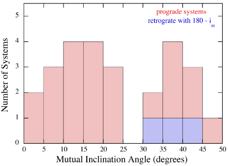
Figure 8: The distribution of mutual orbital inclination angle, $i_{\mathrm{m}}$. In cases where the orbit is retrograde, i.e., $i_{\mathrm{m}}>90\degr$ we have plotted the value $180\degr-i_{\mathrm{m}}$, but indicated those systems with blue shading. There are two fairly clear peaks, one centered near $13\degr$ and the other near $38\degr$. See text for a discussion.

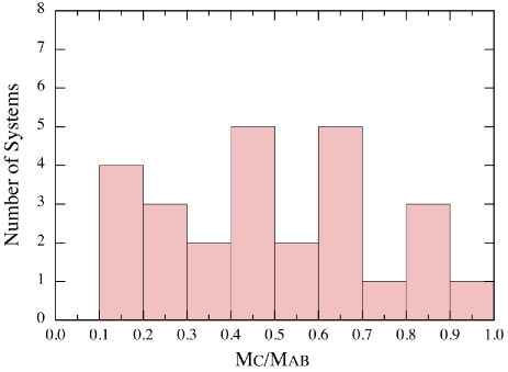
Figure 9: Distribution of the ratio the mass of the third body, $m_{\mathrm{C}}$, to the mass of the inner binary, $m_{\rm AB}$. A ratio of 0.5 corresponds to the case where all three masses in the system could be similar. Only a relative handful of systems have distinctly low-mass tertiary companions; likewise, none has a third body which dominates the system.

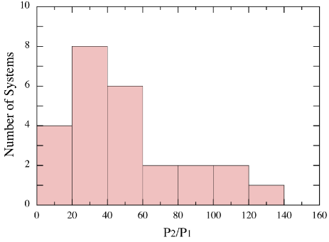
Figure 10: Distribution of the ratio of the outer (triple) period to the inner (binary period, $P_{2}$ vs. $P_{1}$. We have removed one of the 26 systems from this distribution, KIC 10268809, because its outer period greatly exceeds the span of Kepler observations, and is therefore highly uncertain. The bulk of the remaining systems lie in the range $10\lesssim P_{2}/P_{1}\lesssim 100$. The upper limit is a selection effect due to the overall 4-year duration of the Kepler mission.

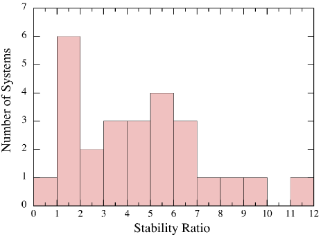
Figure 11: Distribution of the orbital stability ratio, defined as $(P_{2}/P_{1})/(P_{2}/P_{1})_{\rm stab}$, where $P_{2}$ and $P_{1}$ are the triple and binary periods, respectively, and $(P_{2}/P_{1})_{\rm stab}$ is the minimum ratio of these two periods required for stability. We utilize Eqn. (90) from Mardling & Aarseth (2001) for the stability criterion (see text for details).

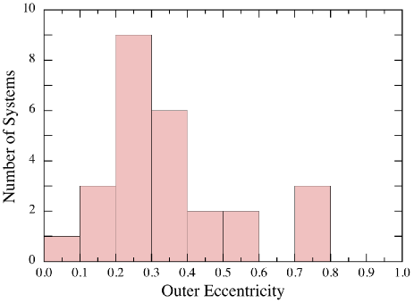
Figure 12: Distribution of the eccentricity of the outer orbit, i.e., that of the triple ($e_{2}$). The triples mostly have modest eccentricities in the range of 0.2–0.5, though 3 of the 26 systems have $e_{2}>0.7$.

Our sample of 26 compact hierarchical triples (CHTs) with well measured system parameters is not large, but is considerably more than has been heretofore available for statistical analysis. It is especially true, if we take into account also the small characteristic sizes, i.e., the short outer period of many of the investigated systems. (The rarity of systems with outer period less than 1000 days was discussed in the Introduction.) Some important relationships among the system parameters that we can examine are the ratios between the outer and inner periods ($P_{2}$ and $P_{1}$), the ratios of masses ($m_{\mathrm{C}}$ and $m_{\mathrm{AB}}$), the mutual inclination angles, $i_{m}$, and eccentricities, in particular that of the outer orbit. We also compare the period ratios, $P_{2}/P_{1}$, with an approximate expression for mass ratios leading to dynamical stability.

We start with the mutual inclination angle (i.e., the angle between the plane of the binary and that of the outer third body). Figure 8 shows the distribution of the mutual inclination angle for our 26 CHTs. The three systems marked in blue are those with retrograde orbits ($i_{\mathrm{m}}>90\degr$), and here we have displayed them as $180\degr-i_{\mathrm{m}}$ for convenience. In spite of the limited statistics, there are two clear groups of systems, one centered at $\sim$$13\degr$ and the other at $\sim$$38\degr$. This seems to be consistent with two populations, one that was born with more coplanar orbits, and which have remained that way over time; the other which was born with potentially quite large mutual inclination angles

$$\sin^{2}i_{\mathrm{m}}>2/5~{}~{}~{}{\rm or}~{}~{}~{}39.2\degr\lesssim i_{\mathrm{m}}\lesssim 140.8\degr$$

and which were subject to the Kozai-Lidov oscillation cycles with tidal damping (Kozai, 1962; Lidov, 1962; Kiseleva et al., 1998; Eggleton & Kiseleva-Eggleton, 2001). In this latter group, the Kozai-Lidov cycles might drive the inner binary to be tighter, and tidal dissipation in that binary can terminate the Kozai-Lidov cycles leading to a preferential set of mutual inclination angles in the range of $35\degr$ to $50\degr$ (see, e.g., Fabrycky & Tremaine, 2007), just what is seen in Fig. 8.

Among the many other measured system parameters, we also consider the ratio of the third body mass to the mass of the inner binary. Figure 9 shows the distribution of $m_{\mathrm{C}}/m_{\mathrm{AB}}$. All the systems have $m_{\mathrm{C}}/m_{\mathrm{AB}}<1$. Otherwise the distribution of $m_{\mathrm{C}}/m_{\mathrm{AB}}$ is flat to within the small-number statistics. Roughly half the systems have $m_{\mathrm{C}}/m_{\mathrm{AB}}=0.55\pm 0.15$ which is consistent, within uncertainties, with all three constituent masses being comparable.

The inner binary periods of the systems we have investigated are between $\sim$4 and 40 days. Note that, according to the convention followed, e.g., by Naoz & Fabrycky (2014) only those systems with $P_{\mathrm{orb}}<16\,\mathrm{d}$ are grouped into the category of “close binaries”. By that strict definition, 11 inner binaries of our sample fall into this category. The outer period range extends from $\sim$90 to $\sim$7000 days, although this latter limit, being substantially longer than the observational interval, is quite approximate. In Figure 10 we plot the distribution of the ratio of the outer (i.e., triple) period to the period of the inner binary. The vast majority of the systems lie in the range of $10\lesssim P_{2}/P_{1}\lesssim 100$. The systems with large ratios of $P_{2}/P_{1}$ are clearly in the dynamically stable regime. However, we next investigate this issue of stability somewhat more quantitatively.

A number of groups have investigated the long-term dynamical stability of hierarchical three-body systems, and have developed approximate ‘empirical’ expressions for stability. Mikkola (2008) conveniently summarizes four of these expressions for stability. Somewhat arbitrarily, we have chosen the expression of Mardling & Aarseth (2001) to use for comparison with our observed period ratios. Their expression can be rewritten as:

$$\left(\frac{P_{2}}{P_{1}}\right)_{\rm stab}\gtrsim 4.68\left(\frac{m_{\mathrm{C}}}{m_{\rm AB}}\right)^{1/10}\frac{(1+e_{2})^{3/5}}{(1-e_{2})^{9/5}}$$ (27)

which holds for a wide range of mass ratios and eccentricities (but note that it depends only on $e_{2}$). Its main limitation is that it is valid specifically only for coplanar orbits, and we apply it to our systems with this caveat in mind. In Figure 11 we show the distribution of the observed ratio ($P_{2}/P_{1}$) in units of the ratio for stability, $(P_{2}/P_{1})_{\rm stab}$ given by Eqn. (27), for our sample of 26 CHTs. One of the systems, KIC 06964043, has a stability ratio only marginally more than unity (1.02), while another, KIC 07668648, has a stability ratio of only 0.77 and, as noted above, it has the smallest ratio of $P_{2}/P_{1}$ at 7.3. The fact, that this system is far from a coplanar configuration, ($i_{\mathrm{m}}\sim 40\degr$) might play an important role in its stability. In any case, the system is manifestly dynamically stable, and so this may just point to some minor limitations of the Mardling & Aarseth (2001) expression. The remaining 24 systems have stability ratios (defined above) as greater than unity.

In this regard, it is also interesting to note that 17 of our 26 CHT systems have outer periods of less than 1000 days, and for 8 of the triples $P_{2}$ is even shorter than one year. Taking into consideration the works of Carter et al. (2011); Derekas et al. (2011); Steffen et al. (2011); Gies et al. (2012); Lee et al. (2013); Rappaport et al. (2013); and Conroy et al. (2014), which have reported an additional 51 secure short outer period triple star systems with $P_{2}<1000$ days in the Kepler field, this brings the total number of such systems to at least 68. Therefore, we can made a crude estimate of the frequency of such short outer-period triples. Accepting the stability criteria of Mardling & Aarseth (2001), and neglecting its eccentricity and mass ratio dependence, the upper limit on the inner period for a 1000 day-long outer orbit becomes $P_{1}\sim 215$ days. The Kepler EB catalog contains 2582 entries of binaries with shorter periods. This inner period limit of 215 days, however, could be further restricted considering the fact that the typical detection method for these short outer period Kepler triples is via an ETV analysis. Based on our experience, in order to have a reliable ETV analysis, at least 15-20 eclipse timing data points from the two eclipses combined are required, though this is being somewhat optimistic. (In our sample, the 38 eclipse times for KIC 10319590 could be considered minimal.) This latter requirement considerably reduces the useable range of $P_{1}$ to $\sim 1/10$th of the Q0–Q17 time-span (as one orbit of the inner binary produces two eclipses), i.e., $P_{1}\lesssim 145$ days. If we consider, however, that a period ratio $P_{2}/P_{1}>20$ is observationally much more typical, we actually need to take into account only eclipsing systems with $P_{1}<50$ days. There are 2458 such entries in the Kepler binary catalog.

From the above discussion we can conclude that, very roughly, 2.7% of Kepler binaries with $P_{1}\lesssim 50$ days have third-body stellar mass companions with relatively short outer periods (i.e., $P_{2}\lesssim 1000$ days). As noted in the Introduction, in a recent paper Tokovinin (2014b) reports the complete lack of ternaries with $P_{2}<1000$ d orbital period in his distance-limited solar-like (or less massive) triples. Since a substantial portion of our triples sample, and similarly of the other reported Kepler triples (referenced above), are supposed to be comprised nearly exclusively of solar- and lower-mass stars (Coughlin et al., 2011), our results seem highly appropriate for comparison with the Tokovinin (2014b) findings. The complete sample of Tokovinin (2014a, b) contains only $\sim$200 binaries with $P<50$ days and, therefore, statistically we would expect only $\sim$6 short-period triples amongst them. Furthermore, there is an evident selection effect (not mentioned in the discussion of Tokovinin, 2014b, although, in a different context, it was discussed in Tokovinin, 2014a), which further reduces the expected number of such short-period triples in his sample. This is so because the discovery probability of a close binary sub-system within a previously known few-hundred day wider binary via radial velocity measurements, is evidently biased toward those systems where the more luminous (and therefore usually the more massive) component forms the close binary. In turn, this is true because, if the secondary component of a wider, single-lined spectroscopic binary (SB1) were a close binary, it could easily remain unnoticed. A good example is HD 181068 which, before the Kepler discovery of its unique triply eclipsing nature (Derekas et al., 2011) was categorized as a simple, “boring” SB1 binary (Guillout et al., 2009). An effect which can further strengthen this bias is that for such a bright ternary as can be found, e.g. both in HD 181068 and KOI-126 (Carter et al., 2011) the photometric signatures of a faint close binary subsystem also would remain hidden from ground-based observations. (Note, these selection effects may also provide a natural explanation for the fact that, amongst more massive binaries, short period ternaries were already known.) Therefore, the absence of $P_{2}<1000$ days system in the Tokovinin (2014b) sample is not in serious disagreement with the frequency of such systems in the substantially larger Kepler sample; but, the question of whether it is a selection effect, or not, still requires further investigation.

Finally, we show in Figure 12 the distribution of the eccentricity of the outer binary, i.e., the triple. The outer eccentricities show significant diversity, from the almost circular outer orbit of KIC 07812175 to those three CHTs: KICs 07670617, 08143170, and 10268809, where $e_{2}>0.7$. The eccentricities of the inner binaries lie in the range of $0.001\lesssim e_{1}\lesssim 0.42$.

In the case of eccentricities (both inner and outer), however, it should keep in mind that our sample has substantial selection and observational biases. First, considering the inner eccentricities, in the extreme limit it is evident that we excluded systems with very nearly circular inner orbits. The negative bias toward the high inner-eccentricity end manifests itself in the fact that the higher the inner eccentricity the larger the possibility of the occurrence of only a single binary eclipse event instead of two, and such systems were also excluded from our analysis. Regarding the outer eccentricities, there are clearly counteracting biases. Since the full amplitudes of the dynamical ETV contributions are proportional to $(1-e_{2}^{2})^{-3/2}$, or even higher (negative) powers, it is evident that a higher outer eccentricity results in a larger amplitude and, therefore, more readily detectable ETV. On the other hand, if the outer period significantly exceeds the duration of the data set, another, counteracting selection effect becomes increasingly important. Namely, for highly eccentric outer orbits, the ETV curves reduce to a spike or jump around periastron passage (the larger $e_{2}$ is, the more narrow in orbital phase and larger in amplitude is this feature). In this case, during most of the outer orbit – in the absence of significant dynamical perturbations – the inner period remains almost constant and, therefore, the ETV curves also become plain and featureless. As a consequence, for systems with an outer period significantly longer than the observing window, the detectability of medium or small outer eccentricity systems mainly depends on the ETV amplitude, while for the high outer eccentricity systems it is more limited by the orbital-phase coverage. (This was nicely illustrated in Figs. 6 and 10 of Borkovits et al. 2011.) Therefore, apart from the inner eccentricity related selection effects, we suspect that there are not many additional Kepler systems with $P_{2}\lesssim 1000$ and medium outer eccentricity, such as KICs 05003117, 09963009, and 1235694 that would have remained undetected in our search, with the possible exception of those having a substantially lower-mass tertiary star. On the other hand, we cannot exclude the presence of undetected high outer eccentricity systems, similar to e.g. KICs 07670617, 08143170, 10268809. Note, a more comprehensive and detailed discussion of the detectability limits and some of the selection effects connected to specific parameters of the ETV curves are given in Borkovits et al. (2011).

We also looked at correlations between $e_{2}$ vs. $e_{1}$, $e_{2}$ vs. $P_{2}$, $e_{2}$ vs. $i_{\mathrm{m}}$, and $e_{1}$ vs. $i_{\mathrm{m}}$, but none of them was particularly statistically significant.

7 Summary and Conclusions

We have analyzed the eclipse timing variations of a sample of 26 eccentric eclipsing binaries in the original Kepler field which were suspected of being members of highly gravitationally interacting, compact, hierarchical triple stellar systems. The investigation has followed a distinctly analytical approach. We have improved and extended the analytical description of the effects of the $P_{2}$-time-scale third-body perturbations on the ETV curve(s) of an eclipsing binary orbiting in a hierarchical configuration (Borkovits et al., 2003, 2011). We have also included, for the first time, the long-timescale octupole and short-timescale quadrupole perturbation terms, and connected them to the longest period apsidal motion and orbital precession effects. For these latter two effects, the quadrupole-level third-body perturbations were also taken into account. Our approach made it possible to simultaneously determine most of the orbital parameters of the inner and the outer binaries, both in the observational and the dynamical frames of references, as well as the complex 3D orientation of the orbits, both with respect to each other and to an Earth-based observer. The model was implemented in a computer code which has also been described in this work.

We used our analytic approach to fitting ETV curves simultaneously for both the primary and secondary eclipses for all 26 of the compact hierarchical triple systems we selected from the Kepler sample. We broke this up into three sub-groups: those with complete information needed for robust determination of the system parameters; those systems that were sufficiently ‘close’ (in the sense of having a small $P_{2}/P_{1}$ ratio) that the analytic model is imperfect; and finally those where the model is quite adequate but either the Kepler data train did not cover a sufficient portion of the outer triple orbit, or some other technical issue limited the determination of some of the system parameters.

Group I Systems: By the use of this analytic approach for representing the ETV curves we were able to determine reliable and robust system parameters for 10 of the 26 systems we analyzed. For those 10 systems (comprising group I), at least one and a half outer orbits were covered by the observations (the outer period range for these systems was $104~{}\mathrm{d}\geq P_{2}\geq 968~{}\mathrm{d}$), and the ratio of the inner and outer periods (with one exception) was $P_{2}/P_{1}>20$. Especially noteworthy from this group is KIC 05255552, which has the longest known outer period among any triply eclipsing hierarchical triple system. With such a long period, it is remarkable that the system parameters can be fairly securely determined with eclipse timing, and without the need for a multiseasonal ground-based RV study.

Group II Systems: Our most “insufficiently modeled” sub-group contains the three most compact systems in our sample. For these systems, our model needs some improvement, especially in regard to describing the secular apsidal motion, in order to obtain a more acceptable solution. The fourth triple in group II, KIC 06964043, has a somewhat larger period ratio ($P_{2}/P_{1}\simeq 22.3$) and hence, semi-major axis ($a_{2}/a_{1}\simeq 9.8$) ratio, but due to its large outer eccentricity ($e_{2}\simeq 0.51$) and therefore, the rather small separation near periastron passage of the outer binary, our model description was also somewhat inadequate. Among this group, KIC 07668648 is unique in having the most ‘compact’ configuration of all such CHTs known, with $P_{2}/P_{1}\simeq 7.3$ and $a_{2}/a_{1}\simeq 4.0$!

Group III Systems: For the remaining 12 triples (our group III systems) the somewhat less robust solutions result mainly from observational, or other technical, reasons. In these systems the observations, with one exception, do not span at least one and a half orbital periods. Despite the less robust solutions, as we have discussed in detail, for most of these systems the inferred parameters are in accord with additional system properties which can be deduced independently from the light curves. This supplemental information includes the directions and the rates of eclipse depth variations, and also the different properties of the primary and secondary eclipses in each system. Therefore, we can conclude, that our results for the group III triples, though less accurate than the group I systems, should still be reliable for most of these systems. Among the Group III systems, KIC 07670617 and KIC 10319590 stand out for having clearly retrograde outer orbits.

Our results confirm the bimodal mutual inclination angle distribution of hierarchical triples with relatively short inner periods, in good agreement with the predictions of Fabrycky & Tremaine (2007), and they therefore, indirectly, support the KCTF theory of the formation of close binary systems. However, we hasten to add that most of the 26 systems we studied (16/26) have relatively low mutual inclination angles, likely formed that way, and were not subject to KCTF. Since Fabrycky & Tremaine (2007) started with an isotropic distribution of mutual inclination angles, it is reasonable that their final distribution would have a minimum at $i_{\mathrm{m}}=0\degr$ since that is the least likely a priori angle to start with. However, to the extent that the initial distribution of $i_{\mathrm{m}}$ is itself bimodal, with a good fraction of the systems (at least those with $P_{\rm 2,init}\lesssim 2000$ days) having $i_{\mathrm{m}}\lesssim 39\degr$, then the final distribution will be a blend of their Fig. 7 with an additional peak at low $i_{\mathrm{m}}$ representing those systems that were born that way (as we see in our Fig. 8).

From among our other statistical results we find, in nearly all cases, that $10\lesssim P_{2}/P_{1}\lesssim 100$. Also, the mass ratios of 19 of the 26 systems in our sample have $1/3\lesssim m_{\mathrm{C}}/m_{\mathrm{AB}}\lesssim 1$, indicating that the third (outer) body is neither particularly massive nor light.

Furthermore, our findings substantially increase the number of the shortest outer period triple systems known and, therefore, can serve as observational probes of the highly underpopulated short-end of the outer period regime of hierarchical triples. These may be essential for understanding the different theories of close binary formation.

Finally, we discuss two issues related to our approach to fitting for orbital solutions in CHTs. First is the omission of such additional information as the eclipse depth and duration variations which can also be deduced from Kepler observations, and which could (in some cases) have dramatically improved our solutions, and/or made them more unique. In one sense this is admittedly a weakness of our approach. On the other hand, the inclusion of such effects into an otherwise fast and analytic method, has both theoretical and practical obstacles. Consider first the eclipse depth variations. In this case, despite the relatively low frequency of the LC measurements, which for most systems results in a very weak sampling of each individual eclipse, the varying depths of the eclipses can be easily measured with considerable accuracy, as was mentioned previously in Sect. 4. We illustrate this for the case of KIC 05731312 in Fig. 13. A substantial difficulty arises, however, from the theoretical side. Namely, the eclipse depth variations are highly sensitive not only to the geometric properties of the inner orbit, but also to stellar parameters such as their radii relative to each other and to the orbital separation, tidally and rotationally distorted shapes, $T_{\rm eff}$, and limb-darkening (see Csizmadia et al. 2013 for a recent study of the influence of limb-darkening models on transiting exoplanet light curve solutions). Furthermore, in the case of partial eclipses, the functional dependences are quite complex and far from trivial (for details, see, e.g., Chapter IV in Kopal 1979).

Turning to the eclipse durations, the problem here is more of a practical one than theoretical. Since the theoretical aspect of eclipse durations was comprehensively studied by Kipping (2010), we comment here only the practical obstacles, i.e. observational aspects, which prevent us from utilizing varying eclipse durations in our fits. The Kepler sampling time of nearly half an hour, in our opinion, makes it very difficult, if not impossible, to find the subtle changes in times of the first and last (or fourth) contacts of each individual eclipse with sufficient accuracy, at least not without the use of an a priori (or, a posteriori) physical-geometrical light curve model which we have intentionally avoided.

Furthermore, regarding our approach to finding orbital solutions for CHTs, we note that the sole use of easily obtainable and accurate eclipse timing data makes our algorithm more generally applicable, not only for Kepler data, but even for non-homogenous observational data sets. For example, ground-based (follow up) observations at different locations and times, and with different instruments, can produce easily comparable and sufficiently accurate mid-eclipse times, with a little effort. By contrast, for measuring the depth of an individual eclipse, and more specifically its duration, a substantially longer observing window is necessary, which may dramatically limit the available events from a given geographical observing site. Furthermore, in the case of eclipse depth measurements, the strong wavelength-dependence also makes them somewhat more difficult to compare with other measurements. In conclusion, the fact that our algorithm is exclusively based on eclipse timing data, makes it readily applicable to any other ETV data.

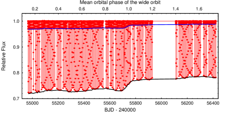
Figure 13: The Kepler light curve of KIC 05731312 (red), which exhibits characteristic, uneven eclipse depth variations. The black and blue lines connect the approximate brightness (relative flux) levels at the mid-eclipse points for primary and secondary eclipses, respectively. Their values were determined as a by-product of the ETV calculations (i.e., eclipse template fitting), as was described in detail in the text. As the out-of-eclipse flux level clearly remains constant during the entire observing interval, these black and blue curves could be directly used for quantifying the eclipse depth variations. Note also, that the red points show the individual LC flux points, and their Moiré pattern helps us to visualize the beating effect between the data sampling frequency and the orbital period. It is apparent that the template-fitting procedure has immunity from this beating effect.

Second in regard to our fitting approach, we note that the orbital solutions, could have been found by direct 3-body numerical integrations coupled to Levenberg-Marquardt and/or MCMC parameter estimation schemes. The advantage of using the admittedly complicated analytic expressions to model the ETV curves is that they provide us with key insight into what kinds of information are required for complete and for partial orbital solutions. The analytical ETV expressions also show us the functional dependences on the various physical parameters of the system. In particular, we now understand how the use of both the primary and secondary ETV curves for an eccentric inner binary can break the near degeneracy between the LTTE and physical delay effects contributing to the ETV curves. In addition, as discussed in the Introduction, fitting ETV curves via an analytic approach is considerably faster than running a numerical integration for many possible system configurations. In the Kepler era and beyond, where there promise to be hundreds of such hierarchical triples, speed in deducing system parameters may be of some importance. A numerical approach to fitting TTVs is likely to remain the appropriate technique in the exoplanet realm, but the analytic approach promises to remain effective for hierarchical triples.

Appendix A Long-term octupole terms

The most common procedure for calculating analytic perturbation formulae in orbital dynamics is the use of canonical equations on perturbations to the Hamiltonian function. For the hierarchical stellar three-body problem, the pioneering work was carried out in a series of papers by Harrington (1968, 1969) who used the renowned von Zeipel averaging technique. For some practical reasons which were enumerated by Borkovits et al. (2003) we followed a different, but equivalent method. Instead of the perturbing potential and, therefore, the Hamiltonian, we calculated the perturbing force. From that, we obtained the direct, analytic perturbation equation for the ETVs with the use of the perturbation equations expressed via the force components (see e.g., Milani et al., 1987). In this Appendix we do not repeat the individual steps (which were described in e.g. Borkovits et al. 2011), and only list the perturbing force up to second order in $a_{1}/a_{2}$, and also give the general final-form of the long-term octupole contribution of the ETV. We felt that these expressions would be too lengthy for inclusion in the main body of the text.

Thus restricting ourselves, the perturbing force components are as follows:

$$\vec{f}=\frac{Gm_{\mathrm{C}}}{\rho_{2}^{3}}\left\{\left[\sum_{n=0}^{\infty}\left(\frac{m_{\mathrm{A}}}{m_{\mathrm{AB}}}\right)^{n}\left(\frac{\rho_{1}}{\rho_{2}}\right)^{n}P_{n}(\lambda)\right]^{3}\vec{r}_{\mathrm{BC}}-\left[\sum_{n=0}^{\infty}(-1)^{n}\left(\frac{m_{\mathrm{B}}}{m_{\mathrm{AB}}}\right)^{n}\left(\frac{\rho_{1}}{\rho_{2}}\right)^{n}P_{n}(\lambda)\right]^{3}\vec{r}_{\mathrm{AC}}\right\}\;,$$ (28)

where $\rho_{1,2}$, are the lengths of the first two Jacobian position vectors (i.e., essentially the separations of the inner and outer binary), $P_{n}$ indicates the $n$-th Lagrangian polynomial, while $\lambda$ is the direction cosine between the (Jacobian) radius vectors ($\vec{\rho}_{1}$ and $\vec{\rho}_{2}$) of the two binaries. The radial, tangential, and normal components of this perturbing force vector up to the octupole order are

$$f_{\mathrm{r}} = \frac{Gm_{\mathrm{C}}}{\rho_{2}^{2}}\left\{2\left(\frac{\rho_{1}}{\rho_{2}}\right)P_{2}(\lambda)+3\frac{m_{\mathrm{A}}-m_{\mathrm{B}}}{m_{\mathrm{A}}+m_{\mathrm{B}}}\left(\frac{\rho_{1}}{\rho_{2}}\right)^{2}P_{3}(\lambda)\right\}~{},$$ (29)

$$f_{\mathrm{t}} = \frac{Gm_{\mathrm{C}}}{\rho_{2}^{2}}\left\{3\left(\frac{\rho_{1}}{\rho_{2}}\right)\lambda+3\frac{m_{\mathrm{A}}-m_{\mathrm{B}}}{m_{\mathrm{A}}+m_{\mathrm{B}}}\left(\frac{\rho_{1}}{\rho_{2}}\right)^{2}\left[\frac{5}{2}\lambda^{2}-\frac{1}{2}\right]\right\}\mu~{},$$ (30)

$$f_{\mathrm{n}} = \frac{Gm_{\mathrm{C}}}{\rho_{2}^{2}}\left\{3\left(\frac{\rho_{1}}{\rho_{2}}\right)\lambda+3\frac{m_{\mathrm{A}}-m_{\mathrm{B}}}{m_{\mathrm{A}}+m_{\mathrm{B}}}\left(\frac{\rho_{1}}{\rho_{2}}\right)^{2}\left[\frac{5}{2}\lambda^{2}-\frac{1}{2}\right]\right\}\nu~{},$$ (31)

respectively, where the direction cosines are

$$\lambda = \cos{w_{1}}\cos{w_{2}}+\sin{w_{1}}\sin{w_{2}}\cos{i}_{\mathrm{m}},$$ (32)

$$\mu = -\sin{w_{1}}\cos{w_{2}}+\cos{w_{1}}\sin{w_{2}}\cos{i}_{\mathrm{m}},$$ (33)

$$\nu = \sin{w_{2}}\sin{i}_{\mathrm{m}}.$$ (34)

A straightforward calculation leads to the following results:

$$f_{\mathrm{r}} = \frac{3}{8}\frac{Gm_{\mathrm{C}}}{\rho_{2}^{2}}\frac{\rho_{1}}{\rho_{2}}\left[(1+I)^{2}\cos(2w_{2}-2w_{1})+(1-I)^{2}\cos(2w_{2}+2w_{1})+2(1-I^{2})(\cos 2w_{1}+\cos 2w_{2})+2\left(I^{2}-\frac{1}{3}\right)\right]$$ (35)

$$+\frac{15}{64}\frac{Gm_{\mathrm{C}}}{\rho_{2}^{2}}\left(\frac{\rho_{1}}{\rho_{2}}\right)^{2}\frac{m_{\mathrm{A}}-m_{\mathrm{B}}}{m_{\mathrm{A}}+m_{\mathrm{B}}}\left\{(1+I)^{3}\cos(3w_{2}-3w_{1})+(1-I)^{3}\cos(3w_{2}+3w_{1})\right.$$

$$+3\left(1-I^{2}\right)\left\{(1+I)\left[\cos(3w_{2}-w_{1})+\cos(w_{2}-3w_{1})\right]+(1-I)\left[\cos(3w_{2}+w_{1})+\cos(w_{2}+3w_{1})\right]\right\}$$

$$\left.-\frac{3}{5}\left(1+11I-5I^{2}-15I^{3}\right)\cos(w_{2}-w_{1})-\frac{3}{5}\left(1-11I-5I^{2}+15I^{3}\right)\cos(w_{2}+w_{1})\right\},$$

$$f_{\mathrm{t}} = \frac{3}{8}\frac{Gm_{\mathrm{C}}}{\rho_{2}^{2}}\frac{\rho_{1}}{\rho_{2}}[(1+I)^{2}\sin(2w_{2}-2w_{1})-(1-I)^{2}\sin(2w_{2}+2w_{1})-2(1-I^{2})\sin 2w_{1}]$$ (36)

$$+\frac{15}{64}\frac{Gm_{\mathrm{C}}}{\rho_{2}^{2}}\left(\frac{\rho_{1}}{\rho_{2}}\right)^{2}\frac{m_{\mathrm{A}}-m_{\mathrm{B}}}{m_{\mathrm{A}}+m_{\mathrm{B}}}\left\{(1+I)^{3}\sin(3w_{2}-3w_{1})-(1-I)^{3}\sin(3w_{2}+3w_{1})\right.$$

$$+\left(1-I^{2}\right)\left\{(1+I)\left[\sin(3w_{2}-w_{1})+3\sin(w_{2}-3w_{1})\right]-(1-I)\left[\sin(3w_{2}+w_{1})+3\sin(w_{2}+3w_{1})\right]\right\}$$

$$\left.-\frac{1}{5}\left(1+11I-5I^{2}-15I^{3}\right)\sin(w_{2}-w_{1})+\frac{1}{5}\left(1-11I-5I^{2}+15I^{3}\right)\sin(w_{2}+w_{1})\right\},$$

$$f_{\mathrm{n}} = \frac{3}{4}\frac{Gm_{\mathrm{C}}}{\rho_{2}^{2}}\frac{\rho_{1}}{\rho_{2}}[2\cos{w_{1}}\sin 2w_{2}\sin{i}_{\mathrm{m}}+(1-\cos 2w_{2})\sin{w_{1}}\sin 2i_{\mathrm{m}}]$$ (37)

$$+\frac{15}{32}\frac{Gm_{\mathrm{C}}}{\rho_{2}^{2}}\left(\frac{\rho_{1}}{\rho_{2}}\right)^{2}\frac{m_{\mathrm{A}}-m_{\mathrm{B}}}{m_{\mathrm{A}}+m_{\mathrm{B}}}\sin i_{\mathrm{m}}\left[(1+I)^{2}\sin(3w_{2}-2w_{1})+(1-I)^{2}\sin(3w_{2}+2w_{1})+2\left(1-I^{2}\right)\sin 3w_{2}\right.$$

$$\left.+\left(1-2I-3I^{2}\right)\sin(w_{2}-2w_{1})+\left(1+2I-3I^{2}\right)\sin(w_{2}+2w_{1})-\frac{6}{5}\left(1-5I^{2}\right)\sin{w_{2}}\right].$$

In each of the three above equations, the first line represents the quadrupole forces, while the others indicate the octupole contributions. We call attention to the last term of the quadrupole contribution to the radial component of perturbation force. This is the only term which does not depend upon any of the $w$ angles, i.e., the relative positions of the bodies with respect to the intersections of the orbital planes, but depends only upon their actual distance ratio. Therefore, it acts to effectively modify the mass of the inner binary in a time-dependent way. However, as far as $I^{2}<1/3$ this extra radial force is always directed outward and results in a reduced mass, and therefore a longer inner binary period, on average, while for highly inclined configurations (i.e., for $\sim 54.736\degr<i_{\mathrm{m}}<\sim 125.264\degr$) the net effect is the opposite. As a natural consequence, around the periastron advance of an eccentric outer binary, (i.e., when the ratio of $\rho_{1}/\rho_{2}$ is the smallest and, therefore this effect is the largest) the lower mutual inclination systems produce a rapid change in time delay, which in the ETV curve morphology manifests itself by a steep and short ascending branch of the sinusoid; several examples of this can be seen in Figs. 2–6. In the opposite sense, eccentric systems with near perpendicular orbits would produce short, steep descending features of the ETV curves, as are illustrated in some figures of Borkovits et al. (2011).

Including these octupole terms into the process described in the above cited papers, we arrive at the following result:

$$\Delta_{\mathrm{2}} = \frac{P_{1}}{2\pi}A_{\mathrm{L2}}\left(1-e_{1}^{2}\right)^{1/2}\left\{2(1+I)\left\{K_{21}{\cal{C}}_{21}(u_{2}-\alpha)+K_{22}{\cal{S}}_{21}(u_{2}-\alpha)-\frac{1}{3}\left[K_{23}{\cal{C}}_{23}(3u_{2}-3\alpha)+K_{24}{\cal{S}}_{23}(3u_{2}-3\alpha)\right]\right\}\right.$$ (38)

$$+2(1-I)\left\{-K_{21}{\cal{C}}_{21}(u_{2}-\beta)+K_{22}{\cal{S}}_{21}(u_{2}-\beta)-\frac{1}{3}\left[-K_{23}{\cal{C}}_{23}(3u_{2}-3\beta)+K_{24}{\cal{S}}_{23}(3u_{2}-3\beta)\right]\right\}$$

$$+\sin^{2}i_{\mathrm{m}}\left\{5(1+I)\left\{-K_{21}{\cal{C}}_{21}(u_{2}-\alpha)-K_{22}{\cal{S}}_{21}(u_{2}-\alpha)+\frac{1}{2}\left[-K_{21}{\cal{C}}_{21}(u_{2}-\beta)+K_{22}{\cal{S}}_{21}(u_{2}-\beta)\right]\right.\right.$$

$$-\frac{1}{10}\left[K_{23}{\cal{C}}_{21}(u_{2}-2\alpha+\beta)+K_{24}{\cal{S}}_{21}(u_{2}-2\alpha+\beta)\right]+\frac{1}{2}\left[K_{21}{\cal{C}}_{23}(3u_{2}-2\alpha-\beta)+K_{22}{\cal{S}}_{23}(3u_{2}-2\alpha-\beta)\right]$$

$$\left.+\frac{1}{15}\left[K_{23}{\cal{C}}_{23}(3u_{2}-3\alpha)+K_{24}{\cal{S}}_{23}(3u_{2}-3\alpha)\right]+\frac{1}{30}\left[-K_{23}{\cal{C}}_{23}(3u_{2}-3\beta)+K_{24}{\cal{S}}_{23}(3u_{2}-3\beta)\right]\right\}$$

$$+5(1-I)\left\{K_{21}{\cal{C}}_{21}(u_{2}-\beta)-K_{22}{\cal{S}}_{21}(u_{2}-\beta)+\frac{1}{2}\left[K_{21}{\cal{C}}_{21}(u_{2}-\alpha)+K_{22}{\cal{S}}_{21}(u_{2}-\alpha)\right]\right.$$

$$+\frac{1}{10}\left[K_{23}{\cal{C}}_{21}(u_{2}-2\beta+\alpha)-K_{24}{\cal{S}}_{21}(u_{2}-2\beta+\alpha)\right]-\frac{1}{2}\left[K_{21}{\cal{C}}_{23}(3u_{2}-2\beta-\alpha)-K_{22}{\cal{S}}_{23}(3u_{2}-2\beta-\alpha)\right]$$

$$\left.\left.\left.+\frac{1}{15}\left[-K_{23}{\cal{C}}_{23}(3u_{2}-3\beta)+K_{24}{\cal{S}}_{23}(3u_{2}-3\beta)\right]+\frac{1}{30}\left[K_{23}{\cal{C}}_{23}(3u_{2}-3\alpha)+K_{24}{\cal{S}}_{23}(3u_{2}-3\alpha)\right]\right\}\right\}\right\}$$

$$+\Delta_{2}^{*}(\sin i_{\mathrm{m}}\cot{i_{1}}).$$

The amplitude of the second order term is

$$A_{\mathrm{L2}}=\frac{m_{\mathrm{A}}-m_{\mathrm{B}}}{m_{\mathrm{AB}}}\left(\frac{m_{\mathrm{AB}}}{m_{\mathrm{ABC}}}\right)^{1/3}\left(\frac{P_{1}}{P_{2}}\right)^{2/3}\frac{A_{\mathrm{L1}}}{1-e_{2}^{2}},$$ (39)

while the integrals of the trigonometric functions of revolution of the wide binary lead to

$${\cal{S}}_{21}(u_{2}) = \left(1+\frac{1}{2}e_{2}^{2}\right)\sin u_{2}+\frac{1}{2}e_{2}\sin(2u_{2}-\omega_{2})+\frac{1}{4}e_{2}^{2}\sin(u_{2}-2\omega_{2})+\frac{1}{12}e_{2}^{2}\sin(3u_{2}-2\omega_{2})+e_{2}\cos\omega_{2}(v_{2}-l_{2}),$$

$${\cal{C}}_{21}(u_{2}) = \left(1+\frac{1}{2}e_{2}^{2}\right)\cos u_{2}+\frac{1}{2}e_{2}\cos(2u_{2}-\omega_{2})-\frac{1}{4}e_{2}^{2}\cos(u_{2}-2\omega_{2})+\frac{1}{12}e_{2}^{2}\cos(3u_{2}-2\omega_{2})-e_{2}\sin\omega_{2}(v_{2}-l_{2}),$$

$${\cal{S}}_{23}(3u_{2}) = \frac{1}{3}\left(1+\frac{1}{2}e_{2}^{2}\right)\sin 3u_{2}+\frac{1}{2}e_{2}\sin(2u_{2}+\omega_{2})+\frac{1}{4}e_{2}\sin(4u_{2}-\omega_{2})+\frac{1}{4}e_{2}^{2}\sin(u_{2}+2\omega_{2})$$

$$+\frac{1}{20}e_{2}^{2}\sin(5u_{2}-2\omega_{2})$$

$${\cal{C}}_{23}(3u_{2}) = \frac{1}{3}\left(1+\frac{1}{2}e_{2}^{2}\right)\cos 3u_{2}+\frac{1}{2}e_{2}\cos(2u_{2}+\omega_{2})+\frac{1}{4}e_{2}\cos(4u_{2}-\omega_{2})+\frac{1}{4}e_{2}^{2}\cos(u_{2}+2\omega_{2})$$ (40)

$$+\frac{1}{20}e_{2}^{2}\cos(5u_{2}-2\omega_{2})$$

Furthermore,

$$K_{21} = \mp\left(\frac{1}{4}+\frac{5}{16}e_{1}^{2}\right)+\frac{57}{80}e_{1}\sin\omega_{1}\pm\frac{5}{16}e_{1}^{2}\cos 2\omega_{1}+\frac{1}{16}e_{1}\sin 3\omega_{1}\mp\frac{1}{16}e_{1}^{2}\cos 4\omega_{1}+{\cal{O}}(e_{1}^{3}),$$

$$K_{22} = -\frac{77}{80}e_{1}\cos\omega_{1}\pm\frac{3}{16}e_{1}^{2}\sin 2\omega_{1}-\frac{1}{16}e_{1}\cos 3\omega_{1}\mp\frac{1}{16}e_{1}^{2}\sin 4\omega_{1}+{\cal{O}}(e_{1}^{3}),$$

$$K_{23} = \pm\frac{105}{16}e_{1}^{2}\cos 2\omega_{1}+{\cal{O}}(e_{1}^{3}),$$

$$K_{24} = \pm\frac{105}{16}e_{1}^{2}\sin 2\omega_{1}+{\cal{O}}(e_{1}^{3}).$$ (41)

Finally, in order to save space in the main body of the text, we list here some additional quantities connected with the quadrupole term, given by Eq. (5). First, there are the quadrupole-level auxiliary functions, $K(e_{1},\omega_{1})$, which we list here up to the seventh order in the inner eccentricity. Second, we give the complete expression for the last term of Eq. (5), i.e., $\Delta_{1}^{*}(\sin i_{\mathrm{m}}\cot{i_{1}})$, which describes those parts of the dynamical perturbations of the ETV which arise directly from the precession of the orbital plane of the inner binary due to an inclined ternary component. Note, since this expression evidently vanishes for coplanar configurations (i.e., when $\sin i_{\mathrm{m}}=0$), it was not worth converting to a form where all the variables would retain their meaning even for $\sin i_{\mathrm{m}}=0$ (as was done for the other components of Eq. [5]). Therefore, the expression below (apart from a corrected sign error) is practically identical to the corresponding part of Eq. (B.15) in Appendix B of Borkovits et al. (2011).

$$\Delta_{1}^{*} = \frac{P_{1}}{2\pi}A_{\mathrm{L1}}\left(1-e_{1}^{2}\right)^{-1/2}\sin i_{\mathrm{m}}\cot{i_{1}}(1-2K_{1})\left\{\left[\frac{2}{5}\left(1+\frac{3}{2}e_{1}^{2}\right)\cos n_{1}-e_{1}^{2}\cos(2\omega_{1}-n_{1})\right]\cos i_{\mathrm{m}}\left[{\cal{M}}-\frac{1}{2}{\cal{S}}(2u_{2}-2n_{2})\right]\right.$$ (42)

$$\left.-\frac{1}{2}\left[\frac{2}{5}\left(1+\frac{3}{2}e_{1}^{2}\right)\sin n_{1}+e_{1}^{2}\sin(2\omega_{1}-n_{1})\right]{\cal{C}}(2u_{2}-2n_{2})\right\}.$$

$$K_{1}(e_{1},\omega_{1}) = \mp e_{1}\sin\omega_{1}+\left(\frac{3}{4}e_{1}^{2}+\frac{1}{8}e_{1}^{4}+\frac{3}{64}e_{1}^{6}\right)\cos 2\omega_{1}\pm\left(\frac{1}{2}e_{1}^{3}+\frac{3}{16}e_{1}^{5}\right)\sin 3\omega_{1}-\left(\frac{5}{16}e_{1}^{4}+\frac{3}{16}e_{1}^{6}\right)\cos 4\omega_{1}$$

$$\mp\frac{3}{16}e_{1}^{5}\sin 5\omega_{1}+\frac{7}{64}e_{1}^{6}\cos 6\omega_{1}+{\cal{O}}(e_{1}^{7}),$$

$$K_{11}(e_{1},\omega_{1}) = \frac{3}{4}e_{1}^{2}+\frac{3}{16}e_{1}^{4}+\frac{3}{32}e_{1}^{6}\pm\left(e_{1}+\frac{1}{2}e_{1}^{3}+\frac{1}{4}e_{1}^{5}\right)\sin\omega_{1}+\left(\frac{51}{40}e_{1}^{2}+\frac{37}{80}e_{1}^{4}+\frac{241}{640}e_{1}^{6}\right)\cos 2\omega_{1}\mp\frac{3}{16}e_{1}^{3}\sin 3\omega_{1}$$

$$-\left(\frac{1}{16}e_{1}^{4}-\frac{1}{16}e_{1}^{6}\right)\cos 4\omega_{1}\mp\frac{1}{16}e_{1}^{5}\sin 5\omega_{1}+\frac{3}{64}e_{1}^{6}\cos 6\omega_{1}+{\cal{O}}(e_{1}^{7}),$$

$$K_{12}(e_{1},\omega_{1}) = \mp\left(e_{1}-\frac{1}{2}e_{1}^{3}-\frac{1}{4}e_{1}^{5}\right)\cos\omega_{1}+\left(\frac{51}{40}e_{1}^{2}+\frac{87}{80}e_{1}^{4}+\frac{541}{640}e_{1}^{6}\right)\sin 2\omega_{1}\mp\frac{3}{16}e_{1}^{3}\cos 3\omega_{1}$$ (43)

$$-\left(\frac{1}{16}e_{1}^{4}+\frac{5}{32}e_{1}^{6}\right)\sin 4\omega_{1}\pm\frac{1}{16}e_{1}^{5}\cos 5\omega_{1}+\frac{3}{64}e_{1}^{6}\sin 6\omega_{1}+{\cal{O}}(e_{1}^{7}).$$

Appendix B Short period terms

For an approximative calculation of the contribution of the short-period terms (i.e., those that contain the inner true anomaly, $v_{1}$ in their arguments) of the perturbation equations, we integrated these terms formally with respect to the true longitude-like quantity ($u_{1}$). To the extent that all the parameters on the right-hand sides of the perturbation equations, with the exception of $v_{1}$ (or $u_{1}$) and $v_{2}$, can be considered to be constant, then the interesting terms take the following forms: $\sin(ku_{1}+nv_{2}+const)(1+e_{2}\cos{v_{2}})^{3}$, or $\cos(ku_{1}+nv_{2}+const)(1+e_{2}\cos{v_{2}})^{3}$, where $k$ is a non-zero integer, while $n=0$, or $n=2$. In order to integrate these equations, we have to express $v_{2}$ as a function of $u_{1}$ (or $v_{1}$). This can be done with two consecutive applications of the Kepler equation, as

$$l_{2}=\frac{P_{1}}{P_{2}}l_{1}+(l_{2})_{0}$$ (44)

and then,

$$v_{2} = l_{2}+2e_{2}\left(1-\frac{e_{2}^{2}}{8}\right)\sin{l_{2}}+\frac{1}{2}e_{2}^{2}\sin 2l_{2}+\frac{3}{8}e_{2}^{3}\sin 3l_{2}+{\cal{O}}\left(e_{2}^{4}\right),$$

$$l_{1} = v_{1}-2e_{1}\sin{v_{1}}+\frac{3}{4}e_{1}^{2}\sin 2v_{1}-\frac{1}{3}e_{1}^{3}\sin 3v_{1}+{\cal{O}}\left(e_{1}^{4}\right).$$ (45)

Then, substituting the corresponding trigonometric functions of $v_{2}$ into the equations, we integrate them formally, and take the lower and upper limits to be $u=u_{0}$ and $u=u_{0}+2\pi N$, where $N$ is an integer (essentially the cycle number), and $u_{0}=\mp\pi$ for the primary and secondary eclipses, respectively.

In such a manner we arrive at the following result:

$$\delta({O-C})_{\mathrm{dir2S}} = \frac{P_{1}}{2\pi}A_{\mathrm{S}}\left(1-e_{1}^{2}\right)^{1/2}\left\{\pm 2e_{1}{\cal{C}}_{0}^{1}(-\omega_{1})-\frac{5}{3}e_{1}^{2}{\cal{S}}_{0}^{2}(-2\omega_{1})\right.$$

$$+(1+I)\left[\frac{11}{15}\left(1-\frac{7}{22}e_{1}^{2}\right){\cal{S}}_{2}^{-2}(2u_{2}-2\alpha)\mp\frac{4}{5}e_{1}{\cal{C}}_{2}^{-1}(2u_{2}-2\alpha-\omega_{1})\right.$$

$$\left.\mp\frac{8}{5}e_{1}{\cal{C}}_{2}^{-3}(2u_{2}-2\alpha+\omega_{1})-\frac{13}{6}e_{1}^{2}{\cal{S}}_{2}^{-4}(2u_{2}-2\alpha+2\omega_{1})\right]$$

$$+(1-I)\left[\frac{11}{15}\left(1-\frac{7}{22}e_{1}^{2}\right){\cal{S}}_{2}^{2}(2u_{2}-2\beta)\pm\frac{4}{5}e_{1}{\cal{C}}_{2}^{1}(2u_{2}-2\beta+\omega_{1})\right.$$

$$\left.\pm\frac{8}{5}e_{1}{\cal{C}}_{2}^{3}(2u_{2}-2\beta-\omega_{1})-\frac{13}{6}e_{1}^{2}{\cal{S}}_{2}^{4}(2u_{2}-2\beta-2\omega_{1})\right]$$

$$+\sin^{2}i_{\mathrm{m}}\left[\mp 3e_{1}{\cal{C}}_{0}^{1}(-\omega_{1})+\frac{5}{2}e_{1}^{2}{\cal{S}}_{0}^{2}(-2\omega_{1})\right.$$

$$+\frac{11}{15}\left(1-\frac{7}{22}e_{1}^{2}\right){\cal{S}}_{0}^{2}(-2n_{1})\pm\frac{4}{5}e_{1}{\cal{C}}_{0}^{1}(\omega_{1}-2n_{1})\pm\frac{8}{5}e_{1}{\cal{C}}_{0}^{3}(-\omega_{1}-2n_{1})-\frac{13}{6}e_{1}^{2}{\cal{S}}_{0}^{4}(-2\omega_{1}-2n_{1})$$

$$\pm\frac{3}{2}e_{1}{\cal{C}}_{2}^{1}(2u_{2}-2n_{2}-\omega_{1})\mp\frac{3}{2}e_{1}{\cal{C}}_{2}^{-1}(2u_{2}-2n_{2}+\omega_{1})-\frac{5}{4}e_{1}^{2}{\cal{S}}_{2}^{2}(2u_{2}-2n_{2}-2\omega_{1})$$

$$-\frac{5}{4}e_{1}^{2}{\cal{S}}_{2}^{-2}(2u_{2}-2n_{2}+2\omega_{1})-\frac{11}{30}\left(1-\frac{7}{22}e_{1}^{2}\right){\cal{S}}_{2}^{-2}(2u_{2}-2\alpha)\pm\frac{2}{5}e_{1}{\cal{C}}_{2}^{-1}(2u_{2}-2\alpha-\omega_{1})$$

$$\pm\frac{4}{5}e_{1}{\cal{C}}_{2}^{-3}(2u_{2}-2\alpha+\omega_{1})+\frac{13}{12}e_{1}^{2}{\cal{S}}_{2}^{-4}(2u_{2}-2\alpha+2\omega_{1})-\frac{11}{30}\left(1-\frac{7}{22}e_{1}^{2}\right){\cal{S}}_{2}^{2}(2u_{2}-2\beta)$$

$$\left.\left.\mp\frac{2}{5}e_{1}{\cal{C}}_{2}^{1}(2u_{2}-2\beta+\omega_{1})\mp\frac{4}{5}e_{1}{\cal{C}}_{2}^{3}(2u_{2}-2\beta-\omega_{1})+\frac{13}{12}e_{1}^{2}{\cal{S}}_{2}^{4}(2u_{2}-2\beta-2\omega_{1})\right]\right\},$$

where

$${\cal{S}}_{0}^{n} = -\frac{\nu}{n^{2}-\nu^{2}}\left[3e_{2}\left(1+3e_{2}^{2}\frac{n^{2}+2\nu^{2}}{n^{2}-4\nu^{2}}\right)\sin v_{2}+3e_{2}^{2}\frac{2n^{2}+\nu^{2}}{n^{2}-4\nu^{2}}\sin 2v_{2}+\frac{3}{2}e_{2}^{3}\frac{3n^{4}+31n^{2}\nu^{2}+8\nu^{4}}{(n^{2}-4\nu^{2})(n^{2}-9\nu^{2})}\sin 3v_{2}\right],$$

$${\cal{C}}_{0}^{n} = \frac{1}{n}\left[1+\frac{3}{2}e_{2}^{2}\frac{n^{2}+\nu^{2}}{n^{2}-\nu^{2}}+3e_{2}\frac{n^{2}}{n^{2}-\nu^{2}}\left(1+\frac{1}{4}e_{2}^{2}\frac{n^{2}+32\nu^{2}}{n^{2}-4\nu^{2}}\right)\cos{v_{2}}+\frac{3}{2}e_{2}^{2}\frac{n^{2}}{n^{2}-\nu^{2}}\frac{n^{2}+5\nu^{2}}{n^{2}-4\nu^{2}}\cos 2v_{2}\right.$$ (47)

$$\left.+\frac{1}{4}e_{2}^{3}\frac{n^{2}}{n^{2}-\nu^{2}}\frac{n^{4}+91n^{2}\nu^{2}+160\nu^{4}}{(n^{2}-4\nu^{2})(n^{2}-9\nu^{2})}\cos 3v_{2}\right]+{\cal{O}}(e_{2}^{4}),$$

$${\cal{S}}_{2}^{n} = \frac{1}{n+2\nu}\left\{\left[1+\frac{1}{2}e_{2}^{2}\frac{3n^{2}-8n\nu-9\nu^{2}}{(n+\nu)(n+3\nu)}\right]\sin 2u_{2}+\frac{1}{2}e_{2}\left[\frac{3n+2\nu}{n+\nu}+\frac{3}{4}e_{2}^{2}\frac{n^{2}-22n\nu-12\nu^{2}}{(n+\nu)(n+3\nu)}\right]\sin(u_{2}+\omega_{2})\right.$$ (48)

$$+\frac{1}{2}e_{2}\left[\frac{3n+2\nu}{n+3\nu}+\frac{3}{4}e_{2}^{2}\frac{n^{3}-42n^{2}\nu-52n\nu^{2}-16\nu^{3}}{(n+\nu)(n+3\nu)(n+4\nu)}\right]\sin(3u_{2}-\omega_{2})$$

$$+\frac{1}{4}e_{2}^{2}\left[\frac{3n+\nu}{n+\nu}\sin 2\omega_{2}+\frac{3n^{2}-5n\nu}{(n+3\nu)(n+4\nu)}\sin(4u_{2}-2\omega_{2})\right]$$

$$\left.-\frac{1}{8}e_{2}^{3}\frac{n^{2}}{(n+\nu)(n-\nu)}\sin(u_{2}-3\omega_{2})+\frac{1}{8}e_{2}^{3}\frac{n^{3}-24n^{2}\nu+24n\nu^{2}}{(n+3\nu)(n+4\nu)(n+5\nu)}\sin(5u_{2}-3\omega_{2})\right\}+{\cal{O}}(e_{2}^{4}),$$

where

$$\nu=\frac{P_{1}}{P_{2}}.$$ (50)

Note that, e.g.

$${\cal{C}}_{0}^{1}(-\omega_{1}) = {\cal{C}}_{0}^{1}\cos\omega_{1}+{\cal{S}}_{0}^{1}\sin\omega_{1},$$

$${\cal{S}}_{2}^{2}(2u_{2}-2\beta) = {\cal{S}}_{2}^{2}\cos 2\beta-{\cal{C}}_{2}^{2}\sin 2\beta.$$ (51)

Appendix C Apsidal motion

While calculating both the LTTE and the $P_{2}$ time-scale perturbations we assumed that the orbital elements remain constant in time. This is not strictly the case; however, it is a plausible approximation for certain restricted intervals, e.g., not substantially longer than the outer period. As is known from the theory of the dynamics of hierarchical triple systems, the highest amplitude periodic perturbations have the longest timescale. The characteristic timescale of these, so-called “apse-node” terms is on the order of $U\sim P_{2}^{2}/P_{1}$ (see e.g., Brown, 1936). For most of the triple stellar systems known before the Kepler–era this timescale exceeds centuries. In sharp contrast to this, the same timescale for some recently discovered systems, which are investigated in this paper, does not exceed 20-30 years. The consequence of this situation is that during the four-year-long observations of Kepler, the argument of periastron ($\omega_{1}$) of such a binary should have changed by $50\degr-70\degr$ (see Table 3). It should also be borne in mind, that these “apse-node” time-scale perturbations are not restricted to apsidal motion and nodal regression, but occur in nearly all the orbital elements (with the exception of the semi-major axes). Here we mainly concentrate on apsidal motion and orbital plane precession, however, a short discussion of other effects will also be presented later.

The angular velocity of the observable apsidal motion (averaged over one binary period) can be written as

$$\dot{\omega}_{1} = \dot{g}_{1}+\dot{n}_{1}$$ (52)

$$= \dot{g}_{1}+\dot{h}_{1}\cos{j_{1}}-\dot{\Omega}_{1}\cos{i_{1}}.$$

Here, the expression on the first row can be seen directly in Fig. 1, while the expression on the second line comes from the theorem of spherical triangles (see Appendix D). Eq. (52) illustrates that the observed apsidal motion will be a combination of the apsidal motion in the dynamical frame, and the nodal regression (or, in other words, precession of the orbital planes). In the following we omit the very last term, because for eclipsing binary orbits viewed nearly edge-on, its contribution is negligible. Restricting ourselves to the quadrupole approximation, the perturbation equations which are the most interesting for us are as follows:

$$\frac{P_{1}}{2\pi}\dot{g}_{1} = A+B\cos 2g_{1},$$ (53)

$$\frac{P_{1}}{2\pi}\dot{h}_{1} = A_{\mathrm{h}}+B_{\mathrm{h}}\cos 2g_{1},$$ (54)

and similarly,

$$\frac{P_{1}}{2\pi}\dot{\omega}_{1} = A_{\mathrm{o}}+B_{\mathrm{o}}\cos 2g_{1},$$ (55)

where

$$A = A_{\mathrm{GR}}+A_{\mathrm{tidal}}+A_{\mathrm{3b}},$$

$$B = B_{\mathrm{3b}}$$ (56)

$$= B_{\mathrm{o}}-B_{\mathrm{n}}.$$

The individual contributions of the relativistic, (equilibrium) tide, and third-body effects are as follows:

$$A_{\mathrm{GR}} = 3\frac{Gm_{\mathrm{AB}}}{c^{2}a_{1}\left(1-e_{1}^{2}\right)},$$ (57)

$$A_{\mathrm{tide}} = \frac{5{\cal{T}}}{2a_{1}^{5}}\frac{1+\frac{3}{2}e_{1}^{2}+\frac{1}{8}e_{1}^{4}}{\left(1-e_{1}^{2}\right)^{5}}+\frac{{\cal{R}}}{a_{1}^{2}\left(1-e_{1}^{2}\right)^{2}},$$ (58)

$$A_{\mathrm{3b}} = A_{\mathrm{sec1}}\left(1-e_{1}^{2}\right)^{-1/2}\left[I^{2}-\frac{1}{5}\left(1-e_{1}^{2}\right)+\frac{2}{5}\left(1+\frac{3}{2}e_{1}^{2}\right)\frac{C_{1}}{C_{2}}I\right],$$ (59)

$$B_{\mathrm{3b}} = A_{\mathrm{sec1}}\left(1-e_{1}^{2}\right)^{-1/2}\left[1-e_{1}^{2}-I^{2}-e_{1}^{2}\frac{C_{1}}{C_{2}}I\right],$$

$$A_{\mathrm{h}} = -\frac{2}{5}\frac{A_{\mathrm{sec1}}}{\cos j_{1}}\frac{1+\frac{3}{2}e_{1}^{2}}{\left(1-e_{1}^{2}\right)^{1/2}}\left(I^{2}+\frac{C_{1}}{C_{2}}I\right),$$ (60)

$$B_{\mathrm{h}} = \frac{A_{\mathrm{sec1}}}{\cos j_{1}}\frac{e_{1}^{2}}{\left(1-e_{1}^{2}\right)^{1/2}}\left(I^{2}+\frac{C_{1}}{C_{2}}I\right),$$ (61)

$$A_{\mathrm{o}} = A+A_{\mathrm{h}}\cos{j_{1}}$$

$$= A_{\mathrm{rel}}+A_{\mathrm{tidal}}+A_{\mathrm{sec1}}\left(1-e_{1}^{2}\right)^{1/2}\frac{3}{5}\left(I^{2}-\frac{1}{3}\right),$$

$$B_{\mathrm{o}} = B+B_{\mathrm{h}}\cos{j_{1}}$$ (63)

$$= A_{\mathrm{sec1}}\left(1-e_{1}^{2}\right)^{1/2}\sin^{2}i_{\mathrm{m}},$$

$$B_{\mathrm{n}} = \cos j_{1}B_{\mathrm{h}}.$$ (64)

Here we have introduced

$$A_{\mathrm{sec1}}=A_{\mathrm{L1}}\frac{P_{1}}{P_{2}}$$ (65)

as the characteristic dimensionless amplitude of the “apse-node” timescale (sometimes called “secular”) quadrupole perturbations. Furthermore, the orbital angular momenta of the two orbits are

$$C_{1} = \frac{m_{\mathrm{A}}m_{\mathrm{B}}}{m_{\mathrm{AB}}}\sqrt{Gm_{\mathrm{AB}}a_{1}\left(1-e_{1}^{2}\right)},$$ (66)

$$C_{2} = \frac{m_{\mathrm{AB}}m_{\mathrm{C}}}{m_{\mathrm{ABC}}}\sqrt{Gm_{\mathrm{ABC}}a_{2}\left(1-e_{2}^{2}\right)},$$ (67)

and, moreover, the coefficients of the (lowest order equilibrium) tidal and (aligned) rotational oblateness are

$${\cal{T}} = 6\left(\frac{m_{\mathrm{B}}}{m_{\mathrm{A}}}k_{2}^{\mathrm{A}}R^{5}_{\mathrm{A}}+\frac{m_{\mathrm{A}}}{m_{\mathrm{B}}}k_{2}^{\mathrm{B}}R^{5}_{\mathrm{B}}\right)$$ (68)

$${\cal{R}} = \frac{k_{2}^{\mathrm{A}}R^{5}_{\mathrm{A}}s^{2}_{\mathrm{A}}}{Gm_{\mathrm{A}}}+\frac{k_{2}^{\mathrm{B}}R^{5}_{\mathrm{B}}s^{2}_{\mathrm{B}}}{Gm_{\mathrm{B}}}.$$ (69)

In the above equations $k_{2}$, $R$ and $s$ refer to the first apsidal motion constants, radii, and rotational angular velocities of stars $A$ and $B$.

By the use of the quantities defined in Eqs. (57–C) we can readily determine the apsidal motion period or, more strictly speaking, approximate timescales for the different contributions to the apsidal motion phenomena. Therefore, the ratio of the dynamical timescale to the sum of relativistic and (simplified, quasi-synchronuously rotating, equilibrium) tidal timescales can be defined as:

$$\frac{P_{\mathrm{GR+tide}}}{P_{\mathrm{3b}}}=\frac{\sqrt{|A_{\mathrm{3b}}^{2}-B_{\mathrm{3b}}^{2}|}}{A_{\mathrm{GR}}+A_{\mathrm{tide}}}.$$ (70)

where the subscript “$\mathrm{3b}$” refers to the dynamically driven apsidal motion. This ratio was calculated for all our system solutions, and is listed in the last column of Table 6. As one can see, the smallest ratio is $\sim 18$, but in most cases it exceeds one hundred, which means that typically the strength of the dynamical effect is two orders of magnitude greater than for the GR and tidal effects. We feel that this nicely justifies our the omission of the non-dynamical contributions to the apsidal motion during the entire analysis.

In contrast to the relativistic and tidal effects, the dynamical apsidal motion comprises a ‘circulating’ (or secular) and a librating (i.e., sine-like) component. We define the amplitude ratio of the two components, as

$$\varepsilon=\frac{B}{A}$$ (71)

(libration over circulation) which can be used for the qualitative description of the main characteristics of the apsidal motion effect. As one can see, for small values of $\varepsilon$, the characteristics of the dynamical apsidal motion remain similar to the tidal, and/or relativistically dominated scenarios, i.e., a (nearly) pure circulation occurs with a well-defined, constant period. The larger the (absolute value of the) ratio, the larger the libration contribution, and for $\varepsilon^{2}=1$ the characteristics of the apsidal motion vary substantially. If we omit the non-third-body contributions, this happens when

$$I^{2}+\frac{1}{5}\left(1+4e_{1}^{2}\right)\frac{C_{1}}{C_{2}}I=\frac{3}{5}\left(1-e_{1}^{2}\right),$$ (72)

which, for the asymptotic approximation of $C_{1}/C_{2}\equiv 0$ recovers the “switching on” condition of the Kozai-Lidov cycles. Note that adding the tidal and relativistic contributions to the dynamical effect usually increases the denominator in $\varepsilon$ and, therefore, reduces its value. Importantly, this may lead to the cancellation of the Kozai-Lidov cycles, as was first pointed out by Söderhjelm (1984).

The $\varepsilon$ parameter however, as well as the individual $A$, $B$ coefficients are primarily dependent on $e_{1}$ and $i_{\mathrm{m}}$, or $j_{1}$ and, therefore, they do not necessarily remain constant in time. The perturbation equations of these latter variables are as follows:

$$\frac{P_{1}}{2\pi}\dot{e}_{1} = e_{1}B_{\mathrm{o}}\sin 2g_{1},$$ (73)

$$\cot j_{1}\frac{P_{1}}{2\pi}\dot{j}_{1} = B_{\mathrm{n}}\sin 2g_{1}.$$ (74)

The form of these equations reveals that, for small inner eccentricities and/or small mutual inclinations, there are only minor variations in these quantities and, therefore also for the right-hand-side coefficients of Eqs. (53–55). Insofar as the right-hand-side coefficients of Eqs. (53–55) and Eqs. (73–74) are considered to be constant, this system of differential equations has simple, closed-form, analytic solutions. This solution was first given in papers by Mazeh & Shaham (1979); Söderhjelm (1982). For $\varepsilon^{2}<1$ the solution takes the following form:

$$g_{1} = \arctan\left(\sqrt{\frac{1+\varepsilon}{1-\varepsilon}}\tan{\cal{G}}\right),$$ (75)

$$h_{1} = {h_{1}}_{0}+\frac{B_{\mathrm{h}}}{B}(g_{1}-{g_{1}}_{0})+\left(A_{\mathrm{h}}-\frac{B_{\mathrm{h}}}{\varepsilon}\right)(u_{1}-{u_{1}}_{0}),$$ (76)

$$e_{1} = {e_{1}}_{0}\sqrt{\left(\frac{1-\varepsilon\cos 2{\cal{G}}}{1-\varepsilon\cos 2{\cal{G}}_{0}}\right)^{B_{\mathrm{o}}/B}},$$ (77)

$$\sin j_{1} = {\sin j_{1}}_{0}\sqrt{\left(\frac{1-\varepsilon\cos 2{\cal{G}}}{1-\varepsilon\cos 2{\cal{G}}_{0}}\right)^{B_{\mathrm{n}}/B}},$$ (78)

and in a similar manner, for the observable argument of periastron

$$\omega_{1} = {\omega_{1}}_{0}+\frac{B_{\mathrm{o}}}{B}(g_{1}-{g_{1}}_{0})+\left(A_{\mathrm{o}}-\frac{B_{\mathrm{o}}}{\varepsilon}\right)(u_{1}-{u_{1}}_{0}).$$ (79)

Here we have introduced the quantity ${\cal{G}}$ which, by formal analogy to the Kepler-problem, can be called the ‘mean dynamical argument of periastron’, and is defined as

$${\cal{G}} = \arctan\left(\sqrt{\frac{1-\varepsilon}{1+\varepsilon}}\tan{g_{1}}\right)$$ (80)

$$= {\cal{G}}_{0}+\Pi(u_{1}-{u_{1}}_{0}),$$

while the apsidal advance rate, averaged over one binary orbit, is

$$\Pi=\sqrt{A^{2}-B^{2}}.$$ (81)

In such a way, the dynamical apsidal motion period becomes

$$P_{\mathrm{g_{1}}}=\frac{P_{1}}{\Pi}.$$ (82)

Eq. (77) reveals that as long as $\varepsilon$ is small, the variation in the inner eccentricity and, similarly for the dynamical inclination, remains small and, therefore in such cases, there are also only minor variations in $\varepsilon$.

There is also a similar analytic solution for the “hyperbolic” case, i.e., when $\varepsilon^{2}>1$; however, we do not list it since, in that case, due to the significant eccentricity variation, the constancy of the right-hand-sides does not hold.

We also note that the equations above are valid, of course, not only for the purely dynamical case, but retain the same form when all the apsidal motion contributions are considered (see Borkovits et al., 2007).

In the next to last column of Table 6 we list the values of $\varepsilon$. For 10 (or 11) systems (naturally, for the lowest mutual inclination triples), this value remains under $0.1$, while for an additional five (or four) systems it is smaller than $0.2$ (or its negative counterpart). On the other hand, most of the remaining systems, for which $0.25<\varepsilon<1.86$, the apsidal advance periods usually are substantially longer than the observational window and, therefore, despite the expected larger variations in the orbital elements and other apsidal motion parameters, a linear approximation over such a relatively short timescale can also be sufficient.

Taking into account the above considerations, our software, in the present case operates in four different apsidal motion calculation modes, as follows:

• Unconstrained, constant apsidal motion rate. In this mode the apsidal advance rate, $\Delta\omega$, is considered to be an independent constant, and can be fitted accordingly.

• Constrained, constant apsidal motion rate. Here the program calculates the instantaneous observed apsidal motion period as

  $$P_{\omega_{1}}=\frac{P_{1}}{A_{\mathrm{o}}+B_{\mathrm{o}}\cos 2(g_{1})_{0}},$$ (83)

  and the variable $\Delta\omega$ is set accordingly. If the apsidal motion rate is also included in the LM process, the software takes into account the functional dependences of this parameter on the other fitted elements, and builds them into the analytical derivatives of the other elements being fitted.

• Constrained, according to the first-order analytical model. In this mode the former Eqs. (75–82), or their large mutual inclination counterparts are used to compute both the observed apsidal motion and the precession rates. Furthermore, the secular variation of $e_{1}$ is also computed, optionally.

Similarly the dynamical precession rate can also be (i) unconstrained, (ii) a constrained constant according to the instantaneous period of

$$P_{\mathrm{h}}=\frac{P_{1}}{A_{\mathrm{h}}+B_{\mathrm{h}}\cos 2(g_{1})_{0}},$$ (84)

or (iii) calculated via the process described above. Then, after obtaining the dynamical precession rate, its realization in the observable quantities is calculated according to the description in the forthcoming Appendix.

Appendix D Constraints of geometry: the spherical triangle(s) formed by inclination angles and nodal arcs

As was mentioned in the main text, the spherical triangle that is formed by the intersections of the two orbital planes and the plane of the sky on the abstract celestial sphere, carries an extraordinary importance in describing and constraining not only the complete three-dimensional configuration of an actual triple system with respect to both its invariable plane, and the observer, but even the orbital dynamics of the triple system. Stirctly speaking we can identify four such triangles in each hemisphere, as is nicely illustrated in Fig. 1. From these eight triangles, in what follows, we choose and discuss the one whose three vertices are the celestial ascending nodes of the two orbits, and consecutive projected intersection of the two orbits. Then, two of the inner vertices are the mutual inclination angle ($i_{\mathrm{m}}$), and one of the observable inclinations, while the other observable inclination becomes the external angle of the third vertex. Moreover, the three arcs are the nodal-like quantities $n_{1}$, $n_{2}$, and also $\Delta\Omega=\Omega_{2}-\Omega_{1}$. Furthermore, with such a choice, the invariable plane of the triple also cuts across our spherical triangle, and divides it into two smaller triangles. In these smaller triangles one arc and vertex are common with the parent triangle (i.e., $n_{1}$ and $i_{1}$, or $n_{2}$ and $i_{2}$), while the corresponding dynamical inclination ($j_{1,2}$) substitutes for $i_{\mathrm{m}}$ and also, the corresponding $\Omega_{1,2}$ (measured arbitrarily from the node of the invariable plane) replaces $\Delta\Omega$, while the third vertices and arcs (i.e., the “other” observable inclination and node are replaced with the “observable” inclination of the invariable plane ($i_{0}$), and dynamical node $h$. (We intentionally omit the subscript for this quantity because it will be the subject of the forthcoming discussion of whether it is $h_{1}$ or $h_{2}$.)

First consider the “large” triangles. From their arcs, both $n_{1}$ and $n_{2}$ occur directly in the perturbation equations. Furthermore, these angles establish a connection between the observable arguments of periastrons $\omega_{1}$ and $\omega_{2}$, from which the first is really an observable (via not only the apsidal part of the ETV analysis, but even with radial velocity measurements or, photometrically, with light-curve analyses), and their dynamical counterparts ($g_{1}$, $g_{2}$), which play a substantial role in the secular dynamics of triple systems (see e.g, Ford et al., 2000). Moreover, as $g_{1}$ is a necessary, important parameter for determining the apsidal advance rate, the spherical triangles constrain even the calculation of the apsidal motion as well (see Appendix C).

Among the angles, $i_{\mathrm{m}}$ is another key parameter not only for the $P_{2}$-timescale perturbations, but also for the secular, or “apse-node”-type perturbation equations. From the two observable inclinations, $i_{1}$ is present directly only in the nodal terms, via its cotangent and, therefore, it has only a weak direct effect on the ETV curves. By contrast, however, the eclipsing nature of our systems yields very strong constraints for its numerical value, which is especially true for the longer period binaries. The outer inclination $i_{2}$ appears directly in the amplitude of the LTTE contribution (via its sine) but, on one hand, this contribution is small, and therefore, has only minor importance for the systems we are investigating, and on the other hand, it also has a complicated and somewhat degenerate connection with the stellar masses and their ratios. In the case of outer-orbit eclipses, however, $i_{2}$ is more strongly constrained than $i_{1}$, due to the substantially larger outer-orbit separations.

As is known from the theory of spherical harmonics, any combinations of the three parameters out of the six constituents determine the given spherical triangle, although, in most configurations, the solution is ambiguous. As a consequence, only three of the five above listed parameters can be set, or adjusted freely, the other two (and also $\Delta\Omega$, not mentioned above) is then already determined (with ambiguity) via the theorem of spherical triangles, and this fact provides strict constraints for our solutions.

The question naturally arises as to which combination(s) are to be used. A complete discussion would be too lengthy to undertake here. Here we show two examples, as follows:

• Systems exhibiting outer-orbit eclipses (free parameters: $i_{2}$, $i_{\mathrm{m}}$, $n_{2}$). In this situation $i_{2}$, $i_{\mathrm{m}}$ and $n_{2}$ were chosen. The presence of outer eclipses very strongly constrains the outer inclination, therefore it can remain reasonably fixed around a value close to $90\degr$, and in such a way controls the physical reliability of the solution. Furthermore, these parameters form one arc and the two vertices lying on that arc of the triangle, which offer one of the simplest computations of the other vertex and arcs. The calculation, however, requires a careful discussion which we present here.

  As was mentioned above, one observable inclination is the inner, and the other is outer angle of the triangle. For example, in the scenario plotted in Fig. 1, $i_{2}$ is the inner, while $i_{1}$ is the outer angle. First we have to resolve this ambiguity. It can also be seen in that figure, that for the illustrated situation $\sin\Delta\Omega<0$. (It also can be shown more generally, that in such a case $-90\degr\leq\Delta\Omega<0\degr$ for prograde, and $180\degr<\Delta\Omega\leq 270\degr$ for retrograde configurations.) Therefore, we can use the sign of $\sin\Delta\Omega$ symbolically, for the separation of the two cases. Thus, our equations will be step-by-step as follows:

  $$\cos{i_{1}}_{a,b} = \cos i_{2}\cos i_{\mathrm{m}}+\mathrm{sgn}(\sin\Delta\Omega)\sin i_{2}\sin i_{\mathrm{m}}\cos n_{2},$$ (85)

  $$\sin{i_{1}}_{a,b} = \sqrt{1-\cos^{2}{i_{1}}_{a,b}},$$ (86)

  $$\sin{n_{1}}_{a,b} = \frac{\sin i_{2}}{\sin{i_{1}}_{a,b}}\sin n_{2},$$ (87)

  $$\sin\Delta\Omega_{a,b} = \mp\frac{\sin i_{\mathrm{m}}}{\sin{i_{1}}_{a,b}}\sin n_{2},$$ (88)

  $$= \mp\frac{\sin i_{\mathrm{m}}}{\sin{i_{2}}}\sin{n_{1}}_{a,b},$$

  $$\cos\Delta\Omega_{a,b} = \frac{\cos i_{\mathrm{m}}-\cos i_{2}\cos{i_{1}}_{a,b}}{\sin i_{2}\sin{i_{1}}_{a,b}},$$ (89)

  $$= \frac{\cos i_{\mathrm{m}}\sin i_{2}-\mathrm{sgn}(\sin\Delta\Omega)\sin i_{\mathrm{m}}\cos i_{2}\cos n_{2}}{\sin{i_{1}}_{a,b}},$$

  $$\cos{n_{1}}_{a,b} = \frac{\cos\Delta\Omega_{a,b}-\sin n_{2}\sin{n_{1}}_{a,b}\cos i_{\mathrm{m}}}{\cos n_{2}},$$ (90)

  $$= \cos n_{2}\cos\Delta\Omega_{a,b}-\sin n_{2}\sin\Delta\Omega_{a,b}\cos i_{2}~{}.$$

  As one can see, in a few cases we have given alternative forms, from which we can choose the one that is more appropriate (e.g., in its numerical behavior). In such a way, we can find two solutions. The software can be set to compute either both solutions, or only one of them; in the program terminology – the “first” (i.e., $\sin\Delta\Omega<0$), or the “second”. (In the case where both calculated solutions are allowed, the program compares the $\chi^{2}$ values, and automatically chooses the better one.) As we shall discuss a bit later, in most cases, one of the solutions results in decreasing eclipse depths with time, while the other in increasing depths. Finally, we also note that similar, but re-labeled equations can be used in the situation where $i_{1}$, $i_{\mathrm{m}}$, $n_{1}$ are chosen.

• Systems with low inner eccentricity and without outer eclipses ($i_{1}$, $i_{\mathrm{m}}$, $n_{2}$). If the outer binary does not produce eclipses, $i_{2}$ is no longer constrained in such a way. Therefore, we can choose $i_{1}$ instead. In such a case, one can choose the set of $i_{1}$, $i_{\mathrm{m}}$ and $n_{1}$ and, therefore similar equations can be applied as before; however, as one can see from Eq. 5, the role of $n_{1}$ and $n_{2}$ is a bit different in the most prominent quadrupole term. Namely, all terms which are connected to $n_{1}$ are multiplied by $e_{1}$ and, therefore, for small inner eccentricities, $n_{1}$ gives only a small contribution. In contrast, the leading $n_{2}$-dependent term remains present even in the doubly circular, non-coplanar case as well. Therefore, it could be better to choose the trio of $i_{1}$, $i_{\mathrm{m}}$ and $n_{2}$. Unfortunately, from the sense of the spherical triangle theorem, this is not among the most fortuitous of cases, and the process becomes somewhat more complex. The steps are as follows:

  $$\sin\Delta\Omega_{a,b} = \mp\frac{\sin i_{\mathrm{m}}}{\sin i_{1}}\sin n_{2},$$ (91)

  $$\cos\Delta\Omega = \sqrt{1-\sin^{2}\Delta\Omega},$$ (92)

  $$\cos{i_{2}}_{a,b} = \frac{\cos i_{1}\cos i_{\mathrm{m}}-\mathrm{sgn}(\sin\Delta\Omega_{a,b})\sin i_{1}\sin i_{\mathrm{m}}\cos\Delta\Omega\cos n_{2}}{1-\sin^{2}n_{1}\sin^{2}i_{\mathrm{m}}},$$ (93)

  $$\sin{i_{2}}_{a,b} = \sqrt{1-\cos^{2}{i_{2}}_{a,b}},$$ (94)

  $$\cos\Delta\Omega = \frac{\cos i_{\mathrm{m}}-\cos i_{1}\cos{i_{2}}_{a}}{\sin i_{1}\sin{i_{2}}_{a}}$$ (95)

  $$= \frac{\cos i_{\mathrm{m}}-\cos i_{1}\cos{i_{2}}_{a}}{\sin i_{1}\sin{i_{2}}_{a}}~{}.$$

  At this step, if $\cos\Delta\Omega<0$ then labels of $i_{2}$ should be interchanged. Finally,

  $$\cos{n_{1}}_{a,b} = \cos\Delta\Omega\cos n_{2}-\sin\Delta\Omega_{a,b}\cos{i_{2}}_{a,b},$$ (96)

  $$\sin{n_{1}}_{a,b} = \frac{\sin{i_{2}}_{a,b}}{\sin i_{1}}\sin n2$$ (97)

  $$= \sqrt{1-\cos^{2}{n_{1}}_{a,b}}~{}.$$

  Note, that for $i_{\mathrm{m}}=n_{2}=90\degr$ the right hand side of Eq. (93) takes the form of zero divided by zero. This situation can happen only when $i_{1}=i_{2}=n_{1}=90\degr$, and $\cos\Delta\Omega=0$, i.e., when the two orbits and the plane of the sky are orthogonal to each other. Such a situation is very far from any of the systems we investigated. Interestingly, on the other hand, the archetypical triple system Algol itself has a configuration not so far from this extreme (see e.g., Zavala et al., 2010,  and further references therein).

Now, we can turn to the other two smaller triangles, which define the position of the invariable plane with respect to the sky, and also make it possible to transform the orbital precession into the observational frame. The unknown vertices and arcs can be calculated, e.g., in the following simple manner.

$$\cos i_{0} = \frac{C_{1}}{C}\cos i_{1}+\frac{C_{2}}{C}\cos i_{2},$$ (98)

$$\sin i_{0} = \sqrt{1-\cos^{2}i_{0}},$$ (99)

$$\cos h = \frac{C_{1}}{C}\frac{\sin i_{1}}{\sin i_{0}}\cos n_{1}+\frac{C_{2}}{C}\frac{\sin i_{2}}{\sin i_{0}},$$ (100)

$$\sin h = \frac{\sin i_{1}}{\sin i_{0}}\sin n_{1}=\frac{\sin i_{2}}{\sin i_{0}}\sin n_{2},$$ (101)

$$\cos j_{1} = \frac{C_{1}}{C_{2}}+\frac{C_{2}}{C}\cos i_{\mathrm{m}},$$ (102)

$$\sin j_{1} = \frac{C_{2}}{C}\sin i_{\mathrm{m}},$$ (103)

$$\cos\Omega_{1} = \frac{C_{1}}{C}\frac{\sin i_{1}}{\sin i_{0}}+\frac{C_{2}}{C}\frac{\sin i_{2}}{\sin i_{0}}\cos\Delta\Omega,$$ (104)

$$j_{2} = i_{\mathrm{m}}-j_{1}~{},$$ (105)

where $C_{1}$, $C_{2}$, as before, denote the absolute value of the inner and outer angular momenta, and the net orbital angular momentum is calculated as:

$$C = C_{2}\sqrt{1+2\frac{C_{1}}{C_{2}}\cos i_{\mathrm{m}}+\left(\frac{C_{1}}{C_{2}}\right)^{2}}~{}.$$ (106)

If once the dynamical inclinations and node are determined, the variations of the observable inclinations ($i_{1}$, $i_{2}$), which are forced by the orbital precession (and which are the direct sources of the eclipse depth variations observed in several systems), can be easily calculated by application of the identities obtained from the theorems of spherical triangles. Namely,

$$\cos i_{1} = \cos i_{0}\cos j_{1}+\mathrm{sgn}(\sin\Delta\Omega)\sin i_{0}\sin j_{1}\cos h,$$ (107)

$$\cos i_{2} = \cos i_{0}\cos j_{2}-\mathrm{sgn}(\sin\Delta\Omega)\sin i_{0}\sin j_{2}\cos h,$$ (108)

$$\sin i_{1} = \sqrt{1-\cos^{2}i_{1}},$$ (109)

$$\sin i_{2} = \sqrt{1-\cos^{2}i_{2}},$$ (110)

$$\sin n_{1} = \frac{\sin i_{0}}{\sin i_{1}}\sin h,$$ (111)

$$\sin n_{2} = \frac{\sin i_{0}}{\sin i_{2}}\sin h,$$ (112)

$$\sin\Omega_{1} = -\mathrm{sgn}(\sin\Delta\Omega)\frac{\sin j_{1}}{\sin i_{1}}\sin h,$$ (113)

$$\sin\Omega_{2} = +\mathrm{sgn}(\sin\Delta\Omega)\frac{\sin j_{2}}{\sin i_{2}}\sin h,$$ (114)

$$\cos\Omega_{1} = \frac{\cos j_{1}-\cos i_{0}\cos i_{1}}{\sin i_{0}\sin i_{1}}=\frac{\cos j_{1}\sin i_{0}-\mathrm{sgn}(\sin\Delta\Omega)\sin j_{1}\cos i_{0}\cos h}{\sin i_{1}},$$ (115)

$$\cos\Omega_{2} = \frac{\cos j_{2}-\cos i_{0}\cos i_{2}}{\sin i_{0}\sin i_{2}}=\frac{\cos j_{2}\sin i_{0}-\mathrm{sgn}(\sin\Delta\Omega)\sin j_{2}\cos i_{0}\cos h}{\sin i_{2}},$$ (116)

$$\cos n_{1} = \frac{\cos\Omega_{1}-\sin h\sin n_{1}\cos j_{1}}{\cos h}=\cos h\cos\Omega_{1}+\sin h\sin\Omega_{1}\cos i_{0},$$ (117)

$$\cos n_{2} = \frac{\cos\Omega_{2}-\sin h\sin n_{2}\cos j_{2}}{\cos h}=\cos h\cos\Omega_{2}-\sin h\sin\Omega_{2}\cos i_{0}~{}.$$ (118)

In the above expression, the meaning of the dynamical node ($h$) requires some additional discussion. First, we had left open the question of whether is it $h_{1}$, or $h_{2}$. The answer, naturally, is that it depends on the sign of $\Delta\Omega$. As far as $\sin\Delta\Omega<0$, as is the case in Fig. 1, the third vertex of the triangle represents the dynamical ascending node of the inner orbit and, therefore $h=h_{1}$, while in the opposite case $h=h_{2}=h_{1}+180\degr$. Another consequence is, that similarly, for the $\sin\Delta\Omega<0$ case $g_{1}=\omega_{1}-n_{1}$, $g_{2}=\omega_{2}-n_{2}-180\degr$, while if $\sin\Delta\Omega>0$ then $g_{1}=\omega_{1}-n_{1}-180\degr$, $g_{2}=\omega_{2}-n_{2}$.

Finally, we use Eq. 107 to enable us to make a few simple, qualitative statements about the eclipse depth variations. Deriving this equation, taking into account that $\dot{\iota_{0}}\equiv 0$, and using additional identities based on the theorems of spherical triangles, we obtain the expressions:

$$\dot{\iota_{1}}=\dot{j_{1}}\cos n_{1}+\mathrm{sgn}(\sin\Delta\Omega)\dot{h}\sin n_{1}\sin j_{1}=\dot{j_{1}}\cos n_{1}-\dot{h}\sin\Omega_{1}\sin i_{0}~{}.$$ (119)

In our simple model we omit the usually small, cyclic variation in the dynamical inclination ($j_{1}$), as well. In such a way, the last term remains. This shows clearly that an alternation between the two ambiguous solutions (discussed above) changes the sign of the variation of $i_{1}$ and, therefore, the observed direction of the eclipse depth variation (if detected) allows us to resolve the ambiguity.

Appendix E Details of the numerical analysis

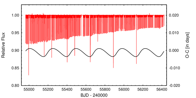
Figure 14: Red curve: The detrended long cadence light curve of KIC 07289157. The varying eclipse depths as well as the ‘anomalous’ outer eclipses are readily discerned. Black curve: The light-time effect (or Roemer delay) contribution to the complete ETV solution. It nicely illustrates that the extra eclipses occur near the extrema of the ETV curve. At the upper extrema events, the third star eclipses one (or both) binary members, while in the lower extrema cases the third star is eclipsed.

In this Appendix we describe in detail how the fits of our analytic ETV functions, with their many system parameters, were fit to the observed ETV curves. We utilize 4 of the 26 triple systems in this study to illustrate how the fitting was done in practice. One of these systems has a low mutual inclination angle, one has a medium inclination angle, while the third is undergoing retrograde motion. The fourth system also has a low mutual inclination angle, but since it is the only triple in our sample where the LTTE term was found to be comparable with the $P_{2}$ timescale quadrupole term, it was chosen for testing the reliability of obtaining individual stellar masses in such a scenario.

E.1 The low mutual inclination regime: the case of KIC 07289157

The triply eclipsing nature of KIC 07289157 makes it extraordinarily useful for testing our analytic fitting model. In Figs. 14 and 15 its long cadence Kepler light curve and ETV curves (determined from the same lightcurves) are shown. The two remarkable features of its light curve are the occurrence of extra, or outer, eclipses and the continuously varying eclipse depths. The period of the cyclic variations of the ETV curve is in accord with the occurrence of the extra eclipses, and clearly reflects the orbital period of the outer binary. The effect of rapid apsidal motion is also readily visible (mostly in the converging primary and secondary ETV curves).

In what follows, we first illustrate the method by which we estimate reliable input parameters for the initial fitting runs. KIC 07289157 has one of the shortest inner periods ($P_{1}\sim 5.27$ days) in our sample. The observable argument of periastron ($\omega_{1}$) and eccentricity ($e_{1}$) of the inner binary can be well approximated from the ETV. The fact that the secondary $O-C$ curve (blue points in Fig. 15) is located below the primary $O-C$ curve indicates that the interval between a primary eclipse and the consecutive secondary eclipse is shorter than half of the binary period, i.e., the periastron passage occurs between the primary and the secondary eclipses. Therefore, $\omega_{1}$ should be located in the fourth or the first quarter, i.e., $-90\degr<\omega_{1}<90\degr$, where the maximum separation occurs at $\omega_{1}=0\degr$ (i.e., when the line of the apsides lies in the plane of the sky). Because the two $O-C$ curves are converging in phase, it follows that in the present situation, as long as we assume prograde apsidal motion, $0\degr<\omega_{1}<90\degr$ is the appropriate quadrant. Therefore, setting $\omega_{1}=45\degr$, we find an appropriate initial guess for the Levenberg-Marquardt (‘LM’) fitting procedure. This latter set of arguments also provides a crude, but satisfactory, initial guess for $e_{1}$, as the separation of the primary and secondary ETVs is related to $\sim 2P_{1}/\pi e_{1}\cos\omega_{1}$. But, as we found, there was no need for this latter estimation for $e_{1}$ since the use of any arbitrary, not-too-extreme initial guess was satisfactory.

Considering the initial parameters for the outer orbit, we have no similar crutches to rely on for its parameter estimations. However, if the $P_{2}$-period contribution to the ETV has a substantially asymmetric shape (which suggests a significant outer eccentricity), the periastron passage time $\tau_{2}$ can be well approximated from the location of the fastest varying portion of the ETV curve. Fortunately, we have found that it was sufficient in most cases to simply guess the correct quadrant for $\omega_{2}$. In other words, we prescribe four initial guesses for the LM fitting of $\omega_{2}$ as $45\degr$, $135\degr$, $225\degr$ and $315\degr$, respectively. Considering the spatial configuration of the system, the triply eclipsing nature gives a very strict constraint on the various inclination angles, especially for $i_{2}$. Namely, for such a long period eclipsing system we expect the outer inclination angle to be very close to $90\degr$. Therefore, although $i_{2}$ has no direct effect on the shape of the ETV, we have chosen that version of the program where $i_{2}$, $i_{\mathrm{m}}$ and $n_{2}$ determine the spatial orientation of the triple system, and therefore, $i_{1}$, $n_{1}$ and $\Delta\Omega$ can no longer be adjusted. Therefore, we set $i_{2}=89.5\degr$. To find an appropriate initial guess for the mutual inclination ($i_{\mathrm{m}}$) we realized that neither the shape of the ETV nor the rate of the eclipse depth variations suggests a substantial mutual inclination angle; therefore, we can set a low initial value, say, between $5\degr$ and $15\degr$, as well as on its retrograde counterparts. On the other hand, we had only a very rough idea for the initial constraints on $n_{2}$; however, we found that six evenly spaced initial values in the range, e.g., $30\degr$ – $180\degr$ could be appropriate.

Finally, some initial estimation of the amplitudes, i.e., masses and mass ratios were also necessary. As is expected, the dominant contribution should be the quadrupole dynamical terms; therefore, its amplitude is the most important. In our experience, setting the $m_{\mathrm{C}}/m_{\mathrm{ABC}}$ parameter to be initially around $1/3$ (which would be the accurate value for three equal masses) was an appropriate choice. Considering the other quantities, related to the LTTE and octupole terms, respectively, we can make some other initial estimates, but they have no crucial significance for the final fit. The Kepler Input Catalog contains the following data for KIC 07289157: $T_{\mathrm{eff}}=6013$ K, $\log g=4.188$, which suggest that the brightest member of the system may be of approximately a solar mass, and a somewhat evolved star. The close binary exhibits very shallow secondary minima, despite the fact that the secondary eclipses are closer to the periastron passage; therefore, it follows that the surface brightness of the secondary star should be low relative to the primary one. If both components are main sequence stars then we may conclude that the secondary might be a faint, M or K star, which results in a small inner mass ratio. On the other hand, the extra anomalous eclipses suggest that the primary and the third, distant star might have similar surface brightnesses. Therefore, as an initial estimate, we assumed that these latter components might have nearly equal masses of $\sim 1$ M_⊙. Thus, we set the appropriate mass parameters accordingly.

In conclusion, in our first trial run the following parameters were adjusted in the LM process: $c_{0}$, $c_{1}$, $e_{1}$, $\omega_{1}$, $P_{2}$, $e_{2}$, $\omega_{2}$ (with 4 initial values), $\tau_{2}$, $m_{\mathrm{C}}/m_{\mathrm{ABC}}$ (with 3 initial values, e.g., in the range of $0.3-0.5$), $i_{\mathrm{m}}$ (1 or 2 initial values), $n_{2}$ (6 initial values). In most cases, such a first run was sufficient to locate the appropriate subspace within the larger parameter space. Then, in the following stages of the fitting, most of the parameters above were also LM-adjusted, but now with better initial values, while additional parameters of $a_{\mathrm{AB}}\sin{i_{2}}$, $q_{1}$, and even $i_{1}$ or $i_{2}$ were also included via the grid-search method. In some systems we obtained a better end-result by disabling the LM-adjustments of $i_{\mathrm{m}}$ and $n_{2}$ during the final fitting, and simply refining them via the grid-search method. In that phase, the grid-searched parameters (i.e., $a_{\mathrm{AB}}\sin{i_{2}}$, $q_{1}$, $i_{\mathrm{m}}$, $n_{2}$ and sometimes $i_{2}$, or $i_{1}$) were used also for controlling the physical reliability of the solutions in an interactive, subjective way. We accepted solutions only with plausible masses and inclinations, and it was also expected that the parameters would be at least marginally consistent with the observed eclipse-depth variations. In the first column of Table 7 we list the main parameters of our solution for KIC 07289157. A more detailed list of the parameters (both adjusted, and derived) obtained from a similar fit, is listed in Tables 3–5. We repeat these results here for an easier comparison with the numerical test results that are described below.

In order to check the reliability of our solutions, we carried out a number of numerical tests. For this (and the forthcoming) numerical integrations we used the code described in Borkovits et al. (2004). Although, our code is able to take into account tidal effects as well, for our present purpose we used simply the three-body point-mass approximation. We generated ETV curves directly from 3-body numerical integrations using the fitted solutions as initial conditions; in the next stage, these were used as “observed” input ETV curves for additional tests of the analytical formulae and fitting processes.

Before any detailed discussion, however, we make note of the difficulty in comparing orbital elements obtained from numerical and analytical solutions. The principal problem is that the analytical formulae (in general) use doubly averaged orbital elements (first for the inner, and then, second, for the outer orbital period), while the numerical integrator, which works directly with the rectangular Jacobian coordinates and velocity vectors, requires instantaneous osculating orbital elements for its initialization. The conversion between the two sets of elements is far from trivial, and would require detailed theoretical considerations. Some short discussion of this issue can be found, e.g., in Kiseleva et al. (1998) and Borkovits et al. (2002). However, this is only of minor importance for our study, and we did not deal with it in full detail, choosing instead to use only a simplified procedure. By the use of the $P_{2}$ time-scale perturbation equations for each orbital element (see, e.g., Eqs. [8]–[15] in Borkovits et al., 2011) we corrected the doubly averaged outputs of our code for $P_{2}$-period perturbations. Then the numerical integrator was initialized with these values. In such an approach, one of the largest amplitude effects was neglected. The remaining other systematic discrepancies which were caused by the incomplete initialization are mainly realized in somewhat different and initial-epoch-dependent orbital and eclipsing periods and phases. However, in conclusion, these discrepancies do not substantially affect any of our main results.

Table 7: Different model solutions for KIC 07289157.

Parameters		OS3	N0F1	N0S3	NsimS3
$P_{1}$	(d)	5.267371	5.268198	5.268189	5.268188
$e_{1}$		0.0849	0.0917	0.0951	0.0957
$\omega_{1}$	($\degr$)	66.018	67.588	68.498	68.638
$\tau_{1}$	(MBJD)	54972.199	54972.233	54972.247	54972.249
$P_{2}$	(d)	243.328	242.595	242.642	242.666
$a_{2}$	(R⊙)	232.047	224.069	231.847	232.438
$e_{2}$		0.309	0.309	0.315	0.317
$\omega_{2}$	($\degr$)	156.330	159.754	157.834	157.669
$\tau_{2}$	(MBJD)	54941.615	54942.569	54941.769	54941.711
$i_{\mathrm{m}}$	($\degr$)	4.630	9.596	5.900	6.191
$i_{1}$	($\degr$)	85.123	99.014	83.859	83.550
$i_{2}$	($\degr$)	89.500	89.500	89.500	89.500
$n_{1}$	($\degr$)	19.071	172.468	17.100	16.104
$n_{2}$	($\degr$)	19.000	172.561	17.000	16.000
$\Delta\Omega$	($\degr$)	1.511	1.252	1.732	1.714
$m_{\mathrm{C}}/m_{\mathrm{ABC}}$		0.388	0.400	0.380	0.379
$m_{\mathrm{B}}/m_{\mathrm{A}}$		0.480	$-$	0.450	0.440
$m_{\mathrm{A}}$	(M⊙)	1.173	1.453	1.217	1.236
$m_{\mathrm{B}}$	(M⊙)	0.563		0.548	0.544
$m_{\mathrm{C}}$	(M⊙)	1.100	0.970	1.079	1.085
$\chi^{2}$		1.9695	0.3183	0.0631	0.3671

Figure 15: The ETV curves for KIC 07289157 (red and blue points for primary and secondary minima, respectively) together with the numerically generated ETV curve with the initial parameters of the OS3 solution of Table 7 (black lines).

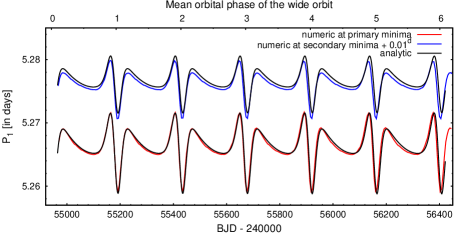
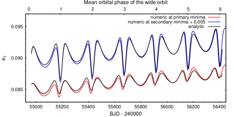
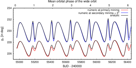
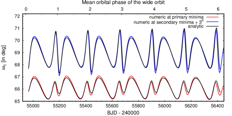
Figure 16: Analytically computed (black), and numerically integrated (red, blue) orbital element variations as a function of time during the OS3 solution, and the equivalent numerical integration for KIC 07289157. Red and blue curves show the osculating instantaneous orbital elements calculated from the integration steps closest to the primary (red) and secondary (blue) eclipses respectively, and demonstrates nicely the phase dependence of such sampling, which can be well modeled by the inclusion of the shortest timescale perturbations (see references in text). The individual panels from left to right, and top to bottom are as follows: first row: instantaneous period (which have short-term contribution exclusively, $P_{1}$); eccentricity ($e_{1}$); second row: the long- and short-term contribution of the dynamical argument of periastron ($g_{1}$); the same for the observable argument of periastron ($\omega_{1}$).

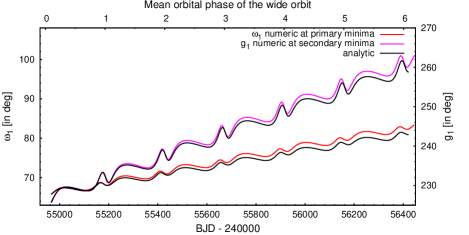
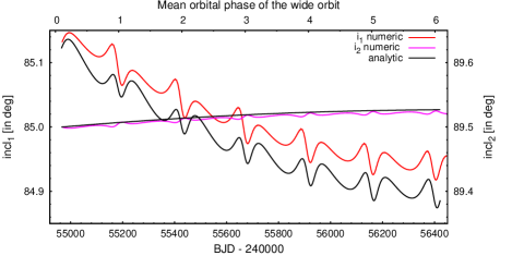
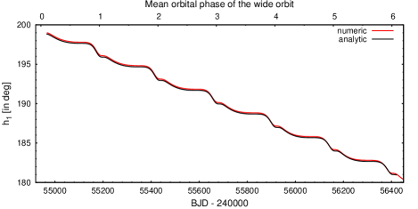
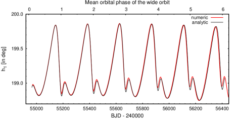
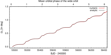
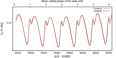
Figure 17: Continuation of Fig. 16. The individual panels from left to right, and top to bottom are as follows: first row: the observable ($\omega_{1}$ – red) and dynamical ($g_{1}$ – magenta) arguments of periastron (where, in order to improve the appearance, the former were sampled at primary eclipses, and the latter at secondary eclipses, only); the observable inclinations ($i_{1}$ – red and $i_{2}$ – magenta); second row: the dynamical node ($h_{1}$); and the same, after subtracting its secular variation; third row: the observable node ($\Delta\Omega_{1}$); and the same, after subtracting its secular variation.

We now turn to the numerical realization of our model solution. In Fig. 15 we plot the observed ETV together with the fitted octupole (or second order) analytic solution. For this particular fit, the third apsidal-motion model was used: ‘OS3’. Some of the inner orbital elements calculated analytically during this process, as well as the same quantities obtained during the numerical integrations, are also plotted in Figs. 16, 17. The numerically generated ETV curves show a somewhat shorter apsidal motion period which manifests itself in a bit faster convergence of the primary and secondary curves. Apart from this feature, it nicely matches the observed, and the analytical ETV as well.

In the additional columns of Table 7 we give analytic solutions, obtained with basically the same procedure, but using either different model approximations, or a different modification of the numerically generated data. Therefore, the Model #N0F1 is a quadrupole (i.e., first-order model, using a constant dynamical apsidal advance rate, which was, however, unconstrained and was applied to the undistorted numerical curve (i.e., $\sigma=0$). Next, Model #N0S3 was an octupole (second order) model, using the advanced apsidal motion modeling, and the same undistorted numerical data. In the case of Model#NsimS3 the same analytic model was applied, however, some simulated noise was added to the numerical data (a random scatter with $\sigma=0.001$ days, and also, 5% of the data points were dropped out randomly).

In conclusion, the comparison of the different solutions reveals that our results for most of the parameters seem to be unique and robust, as was discussed in detail in Sect. 5.2.

Finally, we performed an additional test to check what happens if only either the primary, or the secondary, ETV curves would be fitted. Therefore, similar adjustment processes were applied individually to both the primary and secondary eclipses of both the observed, and the numerically generated data with random added noise. (Note that, in this case, with the absence of any a priori information on apsidal motion, we could not constrain the initial value of $\omega_{1}$, and thus it was initialized with four, evenly spaced values.) The runs were carried out with all apsidal motion modes. The results of the apse mode 3 runs are listed in Table 8, and also plotted in Fig. 18. As one can see, these “results” differ significantly from each other, and also from those which were previously obtained by simultaneously fitting both the primary and secondary ETV curves.

Table 8: Different model solutions for KIC 07289157, when primary and secondary minima were fitted separately.

Parameters		OS3-pri	OS3-sec	NsimS3-pri	NsimS3-sec
$P_{1}$	(d)	5.267728	5.267376	5.263624	5.263611
$e_{1}$		0.0438	0.0902	0.1004	0.1016
$\omega_{1}$	($\degr$)	11.600	118.514	54.614	60.750
$\tau_{1}$	(MBJD)	54971.391	54967.577	54972.000	54972.155
$P_{2}$	(d)	243.303	243.111	242.495	242.424
$a_{2}$	(R⊙)	206.290	219.156	247.960	243.829
$e_{2}$		0.329	0.304	0.321	0.324
$\omega_{2}$	($\degr$)	331.275	189.064	149.997	152.855
$\tau_{2}$	(MBJD)	54948.553	54946.823	54940.403	54941.209
$i_{\mathrm{m}}$	($\degr$)	2.790	2.630	8.384	2.000
$i_{1}$	($\degr$)	91.891	91.883	82.858	91.379
$i_{2}$	($\degr$)	89.500	89.500	89.500	89.500
$n_{1}$	($\degr$)	31.017	25.013	37.824	20.005
$n_{2}$	($\degr$)	31.000	25.000	37.482	20.000
$\Delta\Omega$	($\degr$)	$-1.437$	$-1.112$	5.130	$-0.684$
$m_{\mathrm{C}}/m_{\mathrm{ABC}}$		0.582	0.388	0.371	0.361
$m_{\mathrm{B}}/m_{\mathrm{A}}$		0.430	0.460	0.430	0.470
$m_{\mathrm{A}}$	(M⊙)	0.583	1.003	1.532	1.441
$m_{\mathrm{B}}$	(M⊙)	0.251	0.461	0.659	0.677
$m_{\mathrm{C}}$	(M⊙)	1.159	0.928	1.292	1.196
$P_{\omega_{1}}$	(y)	59.48	92.57	94.01	96.36
$P_{h}$	(y)	56.13	78.94	84.26	83.21
$\chi^{2}$		0.9154	1.5705	0.3103	0.3095

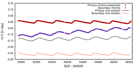
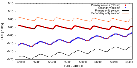
Figure 18: Separately fitted primary and secondary ETV solutions for the observed (left) and the numerically simulated (right) datasets. As one can see, when the primary ETV was used (OS3-pri, NsimS3-pri solutions), the solution fits the primary ETV curves well, but fails to fit the secondary’s ETV curve, and vice versa. See text for further details.

E.2 The medium mutual inclination regime: KIC 08023317 and the retrograde KIC 07670617

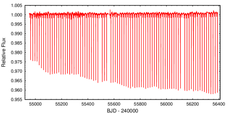
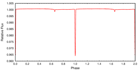
Figure 19: The Q0–Q17 long-cadence light curve of KIC 08023317 (left), and the phased light curve (right).

KIC 08023317 exhibits low-amplitude, but total eclipses of the primary, and remarkably shallower and displaced secondary eclipses. During the 4-years of Kepler observations, the eclipse depth grew continuously (see Fig. 19). Due to the shallowness and flat bottom of the secondary occultations, the times of secondary eclipses were determined with significantly lower accuracy. Therefore, for the case of fitting runs using equal, global ETV uncertainties, which are presented here, we set the value of $\sigma$ for the secondary ETV curve to ten times that of $\sigma$ for the primary curve. Our procedure was similar to that in the previous case, therefore, here we mainly concentrate only on the differences. We kept $i_{1}$ fixed at $89\degr$ due to the implications of total eclipses. Therefore, in this case $i_{\mathrm{m}}$, $n_{2}$ and $i_{1}$ determined the spatial configuration of the triple. The total mass of the system was also initially constrained according to the parameters found in the KIC catalog. In the first three columns of Table 9 we present three different analytic fits which were obtained with different apsidal motion models, i.e., $\Delta\omega$ was considered to be constant and unconstrained (OS1); constant, but constrained (OS2); analytically computed from the first-order secular model (OS3), respectively. Note, in this latter model the program is also able to compute the secular variation of $e_{1}$ from the same analytical model, but after some preliminary checks, we disabled this option. For the first runs, the octupole models led to an unexpectedly high mass ratio ($q_{1}$) for the inner binary. However, we found, that this might be a consequence of the larger timing uncertainties for the secondary ETV curve. We made runs with different ratios of the relative global uncertainty for the secondary and primary ETV curves, and concluded that a smaller weight (i.e., larger uncertainty) for the secondary curve with respect to that of the primary resulted in a lower inner mass ratio. For equal uncertainties we found $q_{1}\approx 4$. Therefore, for the final runs the mass ratio was arbitrarily fixed at $q_{1}=0.5$.

In a further analysis, the parameters obtained from solution OS2 were chosen as initial parameters for the numerical 3-body integration. In the left panel of Fig. 20 the numerical output is plotted against the observed ETV curve. As one can see, while the individual numerical curves fit the corresponding observed curves quite well, the change in their relative displacement, which is a measure of the apsidal motion, varies much more slowly during the numerical integration. The reason can be readily seen in Fig. 21. Although the linear, unconstrained apsidal motion model describes the observable retrograde(!) apsidal motion rate ($\Delta\omega_{1}$) very well, it misses correctly modeling the secular rapid eccentricity variation which would also be necessary for an accurate description of the net relative displacement variations between the primary – secondary ETV curves. Fortunately, the additional fits to the numerically generated curves demonstrate clearly that the derived system parameters have only a minor sensitivity to this effect. The N0S2 column represents the model fit for the numerical ETV curve without added random errors, while the last column lists the solution for another numerical curve with simulated scatter with $\sigma_{\mathrm{pri}}=0.001$ d and $\sigma_{\mathrm{sec}}=0.01$ d. As one can see, apart from the mass parameters, the other quantities remain within a few percent uncertainty, independent of the applied apsidal motion model.

Table 9: Different model solutions for KIC 08023317.

Parameters		OS1	OS2	OS3	N0S2	NsimS2
$P_{1}$	(d)	16.57770	16.57781	16.57903	16.58343	16.58343
$e_{1}$		0.2519	0.2521	0.2558	0.2516	0.2515
$\omega_{1}$	($\degr$)	176.465	175.836	169.046	180.909	180.777
$\tau_{1}$	(MBJD)	54976.758	54976.732	54976.448	54976.951	54976.945
$P_{2}$	(d)	612.051	611.933	611.367	611.525	612.188
$a_{2}$	(R⊙)	347.543	351.101	363.151	357.239	322.756
$e_{2}$		0.2472	0.2476	0.2504	0.2562	0.2649
$\omega_{2}$	($\degr$)	164.132	164.043	161.016	166.552	162.549
$\tau_{2}$	(MBJD)	55010.827	55011.182	55013.239	55010.385	55005.816
$i_{\mathrm{m}}$	($\degr$)	51.962	52.109	52.258	51.015	51.326
$i_{1}$	($\degr$)	89.000	89.000	89.000	89.000	89.000
$i_{2}$	($\degr$)	88.303	87.788	84.197	90.324	89.007
$n_{1}$	($\degr$)	88.627	87.975	83.432	91.227	89.529
$n_{2}$	($\degr$)	89.942	89.545	86.762	91.549	90.486
$\Delta\Omega$	($\degr$)	$-51.973$	$-52.118$	$-52.151$	$-51.000$	$-51.334$
$m_{\mathrm{C}}/m_{\mathrm{ABC}}$		0.086	0.086	0.083	0.095	0.093
$m_{\mathrm{B}}/m_{\mathrm{A}}$		0.500	0.500	0.500	0.570	0.580
$m_{\mathrm{A}}$	(M⊙)	0.917	0.947	1.052	0.944	0.692
$m_{\mathrm{B}}$	(M⊙)	0.458	0.473	0.526	0.538	0.401
$m_{\mathrm{C}}$	(M⊙)	0.130	0.133	0.143	0.156	0.112
$P_{\omega_{1}}$	(y)	$-555.286$	$-609.64$	$-22480.12$	$-569.58$	$-572.24$
$P_{h}$	(y)	699.42	705.30	809.75	628.56	637.45
$\chi^{2}$		0.9494	0.9498	0.9576	0.0016	0.3657

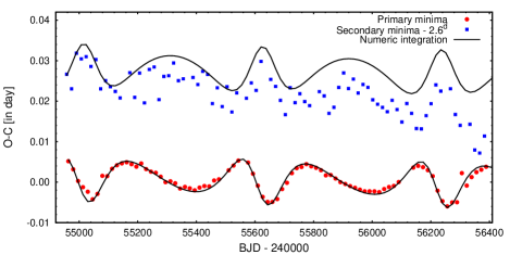
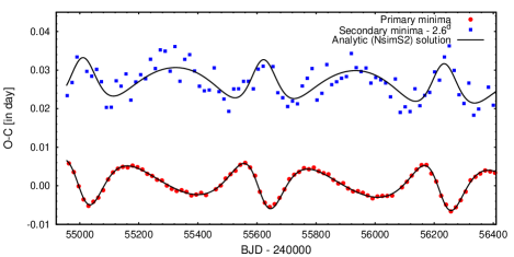
Figure 20: Left panel: The ETV curves of KIC 08023317 (filled red circles and blue boxes for primary and secondary eclipses, respectively) together with the numerically generated ETV curve for which the initial parameters were taken from the analytical Model#OS2 solution (see in Tab. 9) (black lines). Right panel: The same, numerically generated curve with random timing noise added as the “observed” curve to be fitted (red circles and blue boxes), and the analytic “NsimS2” solution (black lines).

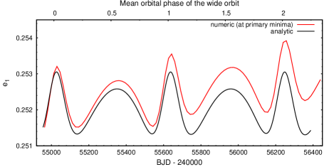
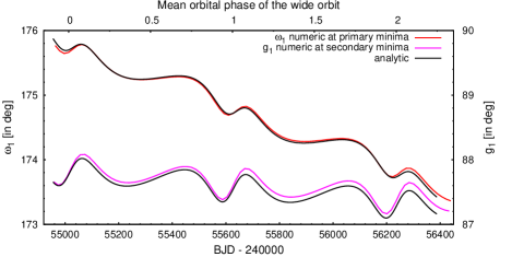
Figure 21: Analytically computed (black), and numerically integrated (red and magenta) orbital element variations for KIC 08023317 during the OS2 solution, and the corresponding numerical integration (NOS2) for KIC 08023317. Note the quick secular change in the eccentricity (left), and also the retrograde observable apsidal motion (right).

Another example of a system with a moderate mutual inclination angle is KIC 07670617. Its ETV is plotted in the fourth panel of Fig. 5. It reveals that the outer orbital period should be substantially longer than the length of the Kepler-observations. However, the marked variations around the periastron passage provides some hope for a satisfactory and reliable fit. The light curve reveals deep primary eclipses, and substantially shallower secondary ones. In the same interval, when the abrupt features occur in the ETVs, the depths of the primary eclipses are suddenly reduced to approximately half of their previous amplitude. Otherwise, the depths remain constant before and after this event. On the other hand, the secondary eclipse ETVs show only a relatively minor variation. Note, this fact suggests that the secondary eclipse should occur closer to periastron passage of the inner binary. The Q0–Q17 long cadence light curve is plotted in the left panel of Fig. 22. In the right panel of the same figure we also plot the variations in the observable inner binary inclination ($i_{1}$) according to our OS1 solution (see below). This figure explains clearly the jump-like behavior seen in the eclipse depth variations.

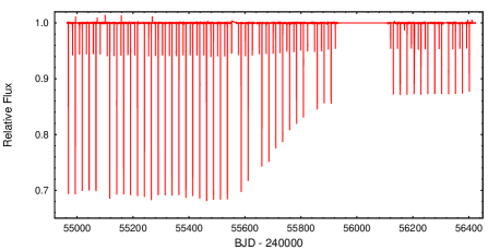
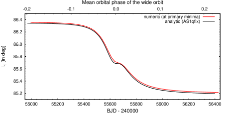
Figure 22: Left panel: The Q0–Q17 long-cadence light curve of KIC 07670617; Right panel: Inner inclination ($i_{1}$) variation of the eclipsing binary, according to the M#OS1qfix solution (see Table 10), and the corresponding numerical integration. This figure explains well the sudden, jump-like eclipse depth variation of the system.

Table 10: Different model solutions for KIC 07670617.

Parameters		OS1	OS1q15	OS3	N01S1	N02P2S1	N02P2S3
$P_{1}$	(d)	24.70493	24.70497	24.70356	24.70666	24.70607	24.70555
$e_{1}$		0.2465	0.2451	0.2318	0.2221	0.2563	0.2405
$\omega_{1}$	($\degr$)	135.852	136.191	140.341	144.606	134.466	138.630
$\tau_{1}$	(MBJD)	54961.528	54961.548	54961.813	54962.118	54961.482	54961.739
$P_{2}$	(d)	3377.992	3047.582	4250.000	3984.191	3378.620	3378.100
$a_{2}$	(R⊙)	1099.766	1093.065	1049.369	1091.749	1099.097	1048.099
$e_{2}$		0.7105	0.6896	0.7565	0.7245	0.7020	0.6913
$\omega_{2}$	($\degr$)	85.463	85.200	82.295	80.294	86.483	87.300
$\tau_{2}$	(MBJD)	55640.396	55638.561	55643.246	55644.075	55646.098	55648.605
$i_{\mathrm{m}}$	($\degr$)	147.174	147.895	143.605	146.158	148.640	149.477
$i_{1}$	($\degr$)	86.000	86.000	86.000	88.000	88.000	89.000
$i_{2}$	($\degr$)	88.987	87.857	94.641	89.735	89.406	94.995
$n_{1}$	($\degr$)	81.889	79.516	87.603	86.538	85.570	96.449
$n_{2}$	($\degr$)	98.981	101.009	89.551	93.988	94.823	85.453
$\Delta\Omega$	($\degr$)	$-147.537$	$-148.469$	143.503	$-146.227$	$-148.743$	$-149.563$
$m_{\mathrm{C}}/m_{\mathrm{ABC}}$		0.391	0.366	0.411	0.431	0.346	0.340
$m_{\mathrm{B}}/m_{\mathrm{A}}$		0.900	15.000	0.900	0.900	0.900	0.900
$m_{\mathrm{A}}$	(M⊙)	0.502	0.075	0.266	0.330	0.538	0.471
$m_{\mathrm{B}}$	(M⊙)	0.452	1.122	0.240	0.297	0.484	0.424
$m_{\mathrm{C}}$	(M⊙)	0.612	0.692	0.353	0.474	0.540	0.461
$P_{\omega_{1}}$	(y)	945.841	953.708	7820.45	902.334	1458.947	2841.64
$P_{h}$	(y)	$-1693.24$	$-1455.80$	$-2157.89$	$-2026.56$	$-2020.12$	$-2238.22$
$\chi^{2}$		1.6999	0.9777	6.2518	0.8536	1.6840	5.2697

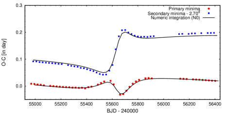
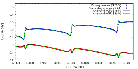
Figure 23: Left panel: The ETV curves of KIC 07670617 (filled red circles and blue boxes for primary and secondary eclipses, respectively) together with the numerically generated ETV curve for which the initial parameters were taken from the analytical Model#OS1 solution (see in Tab. 10) (black lines). Right panel: The numerically generated $\gtrsim 8000$-day long ETV curve with two model solutions (black and green lines).

Figure 24: The secular (and long-term) inner eccentricity ($e_{1}$) and observable argument of periastron ($\omega_{1}$) variation of KIC 07670617 according to the OS1 solution. Red lines represent the results of the numerical integration, while black, magenta and grey stand for the analytically computed values according to the three different apsidal motion models. (See text for detals.)

We present three analytic solutions for this system in the first three columns of Table 10. In the first two cases (OS1 and OS1q15) the apsidal advance rate was an unconstrained, but LM-adjusted constant, while in the third (OS3) it was constrained according to the first order analytic model. In this latter case the secular variation of the inner binary eccentricity was also calculated analytically. Since the inner binary mass ratio tended toward unrealistically high values in all runs (for which the OS1q15 solution is an example), we decided to fix it at $q_{1}=0.9$; however, the significant difference in depths between the primary and secondary eclipses suggests even smaller values. For our follow-up test, the unconstrained apsidal motion solution was used. We generated numerical ETVs with this parameter set both for the same ‘short’ (i.e., Kepler) time interval, and also for an $\sim 8000$ day-long window, which covers more than two outer orbital periods (N0, and N02P2 datasets, respectively). Then, the entire analytic fitting process was reiterated for both the shorter and the longer datasets. The results are tabulated in the third to fifth columns of Table 10, and are shown in Fig. 23. A comparison of the unconstrained apsidal motion solution for the short and the long numerical ETV (N01S1qfix, and N02P2S1qfix) columns reveals that all the orbital elements, including the mutual inclination, $i_{\mathrm{m}}$, remain within $\sim$10% of the other value and, therefore, we may conclude that despite the short observational interval with respect to the orbital period, we can have confidence in our results. On the other hand, the first-order analytical apsidal motion model, unfortunately, seems to be insufficient for describing the secular variations of the orbital elements, even over such a short timescale. In Fig. 24 the variations of $e_{1}$ and $\omega_{1}$ are plotted according to the numerical integration, and the three different apsidal motion models. These panels illustrate clearly that the displacement of the secondary eclipses with respect to the primary eclipses are affected not only by the apsidal advance rate, but by the secular variation of the inner eccentricity. The unconstrained apsidal motion model, therefore, gives a substantially faster apsidal advance rate, for counterbalancing the variation of the eccentricity. The other two apsidal motion models however, result in a more realistic apsidal advance rate. Despite this, in model AP2, due to the absence of eccentricity modeling, this more realistic apsidal advance rate produces only a very poor fit (not listed in Table 10), while in mode AP3 the analytically calculated eccentricity variation results in a somewhat better, but not so good fit. Fortunately, this fact has only a minor influence on fitting the $P_{2}$ timescale terms.

In order to check how certain the retrograde solution is, we constructed numerically a prograde configuration with the same system parameters. It was done by changing $\omega_{2}\rightarrow 180\degr-\omega_{2}$, $i_{2}\rightarrow 180\degr-i_{2}$, $\Omega_{2}\rightarrow\Omega_{2}+180\degr$. Otherwise, the other initial parameters were set according to the OS1 solution. In the first three data columns of Table 11 different solutions are presented. Our findings are a bit contradictory. For the emulated prograde ETV dataset, with duration equal to the Kepler observations, we obtained only a weaker solution (i.e., higher $\chi^{2}$) than for the previously emulated retrograde curve and, furthermore, our fit resulted in a retrograde configuration (although in the same inclination regime). The situation, however, is not as bad as it might seem at first sight. When the inner mass ratio was allowed to take on large, unphysical values, the other solution parameters become much closer to the input values, and the mutual inclination was also changed to the prograde regime column (NproS1q15). As a comparison, during the analysis of the original, Kepler dataset, there was no case where the mutual inclination would have switched to the prograde domain. In the case of the longer simulated prograde dataset, the solution parameters naturally were closer to the initial values, but the solution both in $\chi^{2}$ and the parameter reconstruction, was found to be less robust than in the case of the simulated retrograde dataset.

The origin of the less robust solutions, in our opinion, is to be found in the high outer eccentricity. In order to verify this, we made an additional test. In this case, returning to the retrograde OS1 solution, we modified the outer eccentricity to $e_{2}=0.3$, while all the other parameters were kept at the OS1 values. This run was used not only for testing the high outer eccentricity, but also to check whether the observation of only a single periastron passage in the smaller $e_{2}$ regime may result in sufficient information for parameter recovery. The analytic solution for the $\sim 1450$ day-long $e_{2}=0.3$ ETV curve is presented in the last column of Table 11, and also plotted in Fig. 25. We feel that there is no need for additional comments on the robustness of this latter, smaller eccentricity solution of “KIC 07670617”.

Table 11: Prograde, and smaller outer eccentricity retrograde solutions for KIC 07670617.

Parameters		NproS1	NproS1q15	NproS12P2	Ne23S1
$P_{1}$	(d)	24.70798	24.70485	24.70589	24.70698
$e_{1}$		0.2281	0.2818	0.2854	0.2237
$\omega_{1}$	($\degr$)	142.485	129.270	128.659	143.849
$\tau_{1}$	(MBJD)	54961.980	54961.160	54961.124	54962.056
$P_{2}$	(d)	4000.795	4250.139	3268.371	3312.654
$a_{2}$	(R⊙)	963.460	1220.748	1181.821	979.366
$e_{2}$		0.7441	0.7541	0.7126	0.3012
$\omega_{2}$	($\degr$)	53.213	92.121	90.872	79.529
$\tau_{2}$	(MBJD)	55643.097	55638.951	55638.259	55637.557
$i_{\mathrm{m}}$	($\degr$)	143.489	33.997	33.120	146.766
$i_{1}$	($\degr$)	86.000	86.000	86.000	86.000
$i_{2}$	($\degr$)	88.462	98.700	93.030	88.057
$n_{1}$	($\degr$)	81.972	67.983	78.220	80.285
$n_{2}$	($\degr$)	98.832	69.323	77.937	100.320
$\Delta\Omega$	($\degr$)	$-143.888$	31.628	32.387	$-147.282$
$m_{\mathrm{C}}/m_{\mathrm{ABC}}$		0.519	0.414	0.381	0.434
$m_{\mathrm{B}}/m_{\mathrm{A}}$		0.900	15.000	0.900	0.900
$m_{\mathrm{A}}$	(M⊙)	0.190	0.049	0.676	0.342
$m_{\mathrm{B}}$	(M⊙)	0.171	0.743	0.608	0.308
$m_{\mathrm{C}}$	(M⊙)	0.390	0.561	0.792	0.499
$P_{\omega_{1}}$	(y)	796.945	1414.539	1488.323	1943.051
$P_{h}$	(y)	$-1531.95$	1686.32	1271.16	$-3505.63$
$\chi^{2}$		1.7705	0.6501	3.9799	0.0006

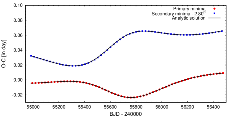
Figure 25: Moderately eccentric ($e_{2}=0.3$) simulated ETV curves for KIC 07670617, and analytical solutions for them. Other initial system parameters were taken from the OS1 solution of Table 10.

E.3 The case of comparable LTTE and dynamical amplitudes: KIC 10268809

Our solution process yielded the longest outer period ($P_{2}=7\,000$ days) for this triple. It is clear that a solution with 5 times longer period than the entire Kepler data set cannot to be taken too seriously. However, this solution yields an LTTE amplitude that is comparable to that of the dynamical quadrupole term (the ratio is $\sim 0.64$; see Table 5). Independent of the reliability of the solution, this makes it possible to probe whether we can obtain reliable individual masses in such cases. Therefore, we numerically integrated the equation of motion for the system according to our solution, and then emulated a $2P_{2}=14\,000$ day-long ETV. Then, this ETV curve was subjected to our parameter finding process. Furthermore, we carried out a second numerical integration, where the only modification to the initial parameters was the reduction of the outer eccentricity from $e_{2}=0.74$ to $e_{2}=0.30$. This was necessary because, as we illustrated above in the case of KIC 10268809, for such a high outer eccentricity our model gives a somewhat weaker solution.

Table 12: Solutions for a 14 000 day-long numerically emulated ETV-s of KIC 102687809.

Parameters		OS1	N2P2S1	N2P2S3	Ne232P2S1	Ne232P2S3
$P_{1}$	(d)	24.70934	24.70917	24.70886	24.70887	24.70879
$e_{1}$		0.3205	0.3126	0.2624	0.3402	0.2889
$\omega_{1}$	($\degr$)	141.505	144.627	168.045	137.854	152.426
$\tau_{1}$	(MBJD)	54965.474	54965.658	54967.067	54965.288	54966.143
$P_{2}$	(d)	7000.000	6999.169	7000.950	7003.080	7000.080
$a_{\mathrm{AB}}\sin i_{2}$	(R⊙)	1000.000	960.156	1058.717	972.894	1012.024
$a_{2}$	(R⊙)	2125.679	1838.509	1712.516	2043.912	2225.400
$e_{2}$		0.7381	0.7403	0.7328	0.3029	0.3334
$\omega_{2}$	($\degr$)	291.841	290.327	303.448	287.244	293.996
$\tau_{2}$	(MBJD)	56147.399	56139.445	56133.369	56116.054	56078.512
$i_{\mathrm{m}}$	($\degr$)	24.300	28.104	28.694	32.259	20.305
$i_{1}$	($\degr$)	84.000	84.000	84.000	84.000	84.000
$i_{2}$	($\degr$)	94.819	92.650	88.310	98.427	81.344
$n_{1}$	($\degr$)	64.020	72.812	97.484	63.729	81.255
$n_{2}$	($\degr$)	63.791	72.013	99.433	64.361	83.872
$\Delta\Omega$	($\degr$)	21.792	26.777	$-28.441$	28.937	$-20.300$
$m_{\mathrm{C}}/m_{\mathrm{ABC}}$		0.472	0.523	0.618	0.481	0.460
$m_{\mathrm{B}}/m_{\mathrm{A}}$		0.700	0.700	0.700	0.700	0.700
$m_{\mathrm{A}}$	(M⊙)	0.818	0.478	0.309	0.713	0.960
$m_{\mathrm{B}}$	(M⊙)	0.572	0.335	0.216	0.500	0.672
$m_{\mathrm{C}}$	(M⊙)	1.243	0.891	0.851	1.125	1.390
$P_{\omega_{1}}$ (unconstrained)	(y)	1904	5333	$-$	20733	$-$
$P_{\omega_{1}}$ (constrained)	(y)	14808	22007	19315	$-207924$	23413
$P_{h}$	(y)	3311	3199	3155	9801	9928
$\chi^{2}$		0.8870	1.2434	3.3243	0.1443	0.9575

In Table 12 we list our solutions obtained with apsidal motion modes AP1 and AP3 both for the “original” and the reduced outer eccentricity numerically emulated ETV. For an easier comparison with the initial parameters we also give the relevant parameters of the $OS1$ solution of the observed ETV. The numerically generated ETVs and the fits are also plotted in Fig. 26. A column-by-column comparison reveals again that our solutions reproduce the initial values for most parameters to within a few percent uncertainty. Furthermore, as was expected, we obtained a better solution for the lower eccentricity case. Now, we concentrate on the individual masses. The two relevant parameters for these are $a_{\mathrm{AB}}\sin{i_{2}}$, which is strongly related to the LTTE amplitude, and the outer mass ratio $m_{\mathrm{C}}/m_{\mathrm{ABC}}$. As one can see for the $e_{2}\sim 0.74$ case, the latter was obtained to within $4-6\%$, while the discrepancy in the $e_{3}=0.3$ case remains $1-3\%$. In contrast, the dynamical amplitudes, and apsidal motion period, which are related to the outer mass ratio, were not well reproduced in the high eccentricity case, but were found to be within $\sim 3\%$ of their actual value in the moderate eccentricity case. Thus, even in this latter case, the resultant discrepancy in the masses remained above $10\%$.

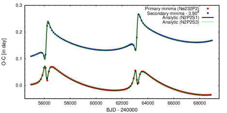
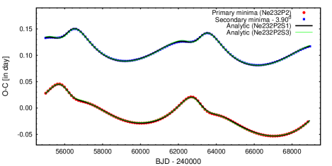
Figure 26: Left panel: Numerically emulated $2P_{2}=14\,000$ day-long ETV curves (red and blue symbols) with the initial parameters of our $OS1$ solution for KIC 10268809, as well as the corresponding analytic fits which are tabulated in Table 12. Right panel: The same, but the outer eccentricity was reduced to $e_{2}=0.3$. Note, for the sake of clarity, only every fifth eclipse point is displayed.

In conclusion, we can state that for comparable magnitudes of the dynamical and LTTE terms, we can deduce individual masses from our fitting process; however, only with moderate accuracy.

Appendix F Tables of Determined Times of Minima for all the 26 Systems

In this Appendix we tabulate the individual $O-C$ times for each of the primary and secondary eclipses for all 26 compact hierarchical triple systems that we considered in this study. The uncertainty in each individual $O-C$ determination is also listed.

Table 13: Times of minima of KIC 04940201

BJD	Cycle	std. dev.	BJD	Cycle	std. dev.	BJD	Cycle	std. dev.
$-2\,400\,000$	no.	$(d)$	$-2\,400\,000$	no.	$(d)$	$-2\,400\,000$	no.	$(d)$
54967.284492	0.0	0.000084	55359.628854	44.5	0.000161	55923.876985	108.5	0.000157
54971.702667	0.5	0.000164	55364.027915	45.0	0.000080	55928.280615	109.0	0.000060
54976.103341	1.0	0.000084	55368.444204	45.5	0.000160	55932.696764	109.5	0.000157
54980.519311	1.5	0.000184	55465.415898	56.5	0.000140	55937.099270	110.0	0.000075
54984.919328	2.0	0.000073	55469.816917	57.0	0.000062	55941.515436	110.5	0.000173
54989.333952	2.5	0.000162	55474.230689	57.5	0.000162	55945.916169	111.0	0.000076
54993.734766	3.0	0.000076	55478.633088	58.0	0.000064	55963.554880	113.0	0.000073
55006.966058	4.5	0.000119	55483.048542	58.5	0.000142	55967.970412	113.5	0.000162
55011.363288	5.0	0.000049	55487.449869	59.0	0.000066	55972.372651	114.0	0.000074
55020.180841	6.0	0.000054	55491.864241	59.5	0.000136	55976.788430	114.5	0.000197
55024.594979	6.5	0.000111	55496.265734	60.0	0.000082	55981.192086	115.0	0.000074
55028.995727	7.0	0.000055	55500.679656	60.5	0.000150	55985.609039	115.5	0.000175
55033.413502	7.5	0.000106	55505.082196	61.0	0.000062	55990.010064	116.0	0.000072
55037.812049	8.0	0.000051	55509.498587	61.5	0.000140	55998.826803	117.0	0.000072
55042.227525	8.5	0.000112	55513.897650	62.0	0.000061	56003.244746	117.5	0.000162
55046.627394	9.0	0.000050	55518.314831	62.5	0.000157	56007.643984	118.0	0.000073
55051.042487	9.5	0.000111	55522.715918	63.0	0.000064	56012.059741	118.5	0.000158
55055.443266	10.0	0.000050	55527.129964	63.5	0.000142	56016.461002	119.0	0.000074
55059.856765	10.5	0.000123	55531.532749	64.0	0.000064	56020.877213	119.5	0.000220
55068.673158	11.5	0.000116	55535.949192	64.5	0.000164	56025.278151	120.0	0.000067
55073.074668	12.0	0.000049	55540.349457	65.0	0.000065	56029.693367	120.5	0.000148
55077.488032	12.5	0.000095	55544.766723	65.5	0.000144	56034.093351	121.0	0.000072
55081.890777	13.0	0.000052	55549.166670	66.0	0.000064	56038.509582	121.5	0.000161
55086.303400	13.5	0.000114	55571.218675	68.5	0.000179	56042.909991	122.0	0.000069
55090.706660	14.0	0.000051	55575.620435	69.0	0.000080	56047.324232	122.5	0.000157
55095.120090	14.5	0.000141	55580.036849	69.5	0.000185	56051.724921	123.0	0.000069
55099.521768	15.0	0.000069	55584.438707	70.0	0.000088	56056.139575	123.5	0.000150
55103.936814	15.5	0.000143	55588.855229	70.5	0.000155	56060.540829	124.0	0.000072
55108.337903	16.0	0.000071	55593.257959	71.0	0.000073	56064.957717	124.5	0.000182
55112.753597	16.5	0.000142	55597.674720	71.5	0.000206	56069.355890	125.0	0.000069
55117.154966	17.0	0.000068	55602.075956	72.0	0.000082	56073.772395	125.5	0.000159
55121.570032	17.5	0.000147	55606.492614	72.5	0.000161	56082.587816	126.5	0.000163
55125.969284	18.0	0.000073	55610.895321	73.0	0.000089	56086.988161	127.0	0.000068
55130.385302	18.5	0.000148	55615.311154	73.5	0.000206	56091.402507	127.5	0.000156
55134.786689	19.0	0.000065	55619.714070	74.0	0.000078	56095.802983	128.0	0.000069
55139.202356	19.5	0.000151	55624.130098	74.5	0.000159	56100.216874	128.5	0.000185
55143.603625	20.0	0.000066	55628.531273	75.0	0.000072	56104.618551	129.0	0.000073
55148.019136	20.5	0.000156	55632.948534	75.5	0.000163	56210.408283	141.0	0.000059
55152.419576	21.0	0.000071	55641.764685	76.5	0.000151	56214.821157	141.5	0.000137
55156.835952	21.5	0.000166	55646.165970	77.0	0.000070	56219.223073	142.0	0.000071
55161.236746	22.0	0.000068	55650.580385	77.5	0.000166	56223.638994	142.5	0.000144
55165.652250	22.5	0.000155	55654.982093	78.0	0.000069	56228.040625	143.0	0.000061
55170.054261	23.0	0.000072	55659.397566	78.5	0.000166	56232.455500	143.5	0.000139
55174.469629	23.5	0.000140	55663.797862	79.0	0.000072	56236.857288	144.0	0.000065
55178.869637	24.0	0.000087	55668.214889	79.5	0.000166	56241.271371	144.5	0.000144
55187.687885	25.0	0.000073	55672.614043	80.0	0.000071	56245.671302	145.0	0.000076
55192.103384	25.5	0.000165	55677.029095	80.5	0.000149	56254.490329	146.0	0.000064
55196.505509	26.0	0.000081	55681.430162	81.0	0.000074	56258.905731	146.5	0.000145
55200.922636	26.5	0.000165	55685.844928	81.5	0.000167	56263.306615	147.0	0.000066
55205.323856	27.0	0.000077	55690.245702	82.0	0.000073	56267.723453	147.5	0.000133
55209.741053	27.5	0.000157	55694.661330	82.5	0.000151	56272.124455	148.0	0.000066

Table 13: Times of minima of KIC 04940201 (continued)

BJD	Cycle	std. dev.	BJD	Cycle	std. dev.	BJD	Cycle	std. dev.
$-2\,400\,000$	no.	$(d)$	$-2\,400\,000$	no.	$(d)$	$-2\,400\,000$	no.	$(d)$
55214.141172	28.0	0.000086	55699.061007	83.0	0.000069	56276.541128	148.5	0.000149
55218.559018	28.5	0.000157	55703.476861	83.5	0.000156	56280.941097	149.0	0.000062
55222.961795	29.0	0.000085	55707.877434	84.0	0.000071	56285.356786	149.5	0.000143
55227.376697	29.5	0.000154	55712.292798	84.5	0.000176	56289.758976	150.0	0.000065
55236.197744	30.5	0.000171	55716.692618	85.0	0.000070	56294.176238	150.5	0.000136
55240.598897	31.0	0.000074	55721.105992	85.5	0.000153	56298.577361	151.0	0.000061
55245.015519	31.5	0.000171	55725.508294	86.0	0.000070	56302.992448	151.5	0.000137
55249.416989	32.0	0.000072	55729.922947	86.5	0.000166	56307.394676	152.0	0.000072
55253.833420	32.5	0.000162	55734.324381	87.0	0.000070	56325.032338	154.0	0.000073
55258.235196	33.0	0.000080	55738.738070	87.5	0.000151	56329.449748	154.5	0.000154
55262.650619	33.5	0.000164	55835.711007	98.5	0.000138	56333.852270	155.0	0.000077
55267.053165	34.0	0.000080	55840.112142	99.0	0.000063	56338.267638	155.5	0.000166
55271.468701	34.5	0.000167	55844.527580	99.5	0.000140	56342.670487	156.0	0.000068
55280.286106	35.5	0.000167	55848.927854	100.0	0.000070	56347.087209	156.5	0.000149
55284.687177	36.0	0.000079	55853.343649	100.5	0.000148	56351.488043	157.0	0.000073
55289.102396	36.5	0.000150	55857.744993	101.0	0.000065	56355.903669	157.5	0.000169
55293.502995	37.0	0.000073	55862.159218	101.5	0.000138	56360.305982	158.0	0.000070
55297.918678	37.5	0.000165	55866.561172	102.0	0.000063	56364.722748	158.5	0.000161
55302.318984	38.0	0.000073	55870.976535	102.5	0.000142	56369.124239	159.0	0.000073
55306.735131	38.5	0.000160	55875.378247	103.0	0.000068	56373.539127	159.5	0.000162
55311.134939	39.0	0.000074	55879.793178	103.5	0.000132	56377.940331	160.0	0.000069
55315.551172	39.5	0.000164	55884.193411	104.0	0.000064	56382.355157	160.5	0.000150
55319.950840	40.0	0.000081	55888.610103	104.5	0.000151	56386.756723	161.0	0.000071
55324.367747	40.5	0.000180	55893.011182	105.0	0.000064	56395.572705	162.0	0.000067
55328.768027	41.0	0.000094	55897.428068	105.5	0.000147	56399.987483	162.5	0.000157
55333.180973	41.5	0.000168	55901.828770	106.0	0.000069	56404.388007	163.0	0.000065
55341.998376	42.5	0.000161	55906.243323	106.5	0.000143	56408.803549	163.5	0.000150
55346.398335	43.0	0.000077	55910.645582	107.0	0.000064	56413.203597	164.0	0.000071
55350.812491	43.5	0.000154	55915.060583	107.5	0.000136	56422.020410	165.0	0.000068
55355.214257	44.0	0.000071	55919.463838	108.0	0.000065

Table 14: Times of minima of KIC 05255552

BJD	Cycle	std. dev.	BJD	Cycle	std. dev.	BJD	Cycle	std. dev.
$-2\,400\,000$	no.	$(d)$	$-2\,400\,000$	no.	$(d)$	$-2\,400\,000$	no.	$(d)$
54970.588895	0.0	0.000208	55443.010892	14.5	0.000151	55911.806709	29.0	0.000238
54988.785838	0.5	0.000146	55457.395193	15.0	0.000227	55930.412697	29.5	0.000172
55003.039896	1.0	0.000221	55475.468042	15.5	0.000172	55944.275563	30.0	0.000216
55021.256127	1.5	0.000160	55489.829350	16.0	0.000241	55962.854231	30.5	0.000167
55035.504910	2.0	0.000231	55507.932891	16.5	0.000168	55976.742813	31.0	0.000205
55053.705977	2.5	0.000162	55522.259406	17.0	0.000251	56009.207289	32.0	0.000187
55067.972251	3.0	0.000236	55540.407516	17.5	0.000185	56157.492627	36.5	0.000151
55086.147349	3.5	0.000154	55572.892603	18.5	0.000160	56171.489481	37.0	0.000193
55118.585610	4.5	0.000190	55587.107739	19.0	0.000238	56189.936612	37.5	0.000145
55132.901107	5.0	0.000274	55605.397928	19.5	0.000158	56203.938574	38.0	0.000184
55151.022416	5.5	0.000181	55619.530941	20.0	0.000236	56222.382073	38.5	0.000174
55165.361708	6.0	0.000244	55749.666688	24.0	0.000192	56236.385651	39.0	0.000228
55197.818946	7.0	0.000250	55767.777014	24.5	0.000146	56254.829141	39.5	0.000179
55215.899455	7.5	0.000179	55782.073916	25.0	0.000186	56287.278866	40.5	0.000179
55248.338674	8.5	0.000158	55800.421943	25.5	0.000141	56301.271738	41.0	0.000223
55262.726848	9.0	0.000218	55814.455652	26.0	0.000202	56333.711334	42.0	0.000200
55378.108730	12.5	0.000149	55832.992513	26.5	0.000141	56352.192770	42.5	0.000161
55392.514806	13.0	0.000230	55846.882849	27.0	0.000237	56366.146325	43.0	0.000192
55410.558854	13.5	0.000156	55879.339308	28.0	0.000250	56384.658283	43.5	0.000146
55424.956175	14.0	0.000215	55897.961642	28.5	0.000192

Table 15: Times of minima of KIC 05653126

BJD	Cycle	std. dev.	BJD	Cycle	std. dev.	BJD	Cycle	std. dev.
$-2\,400\,000$	no.	$(d)$	$-2\,400\,000$	no.	$(d)$	$-2\,400\,000$	no.	$(d)$
54985.877118	0.0	0.001065	55693.781088	18.5	0.007507	56063.792943	28.0	0.000618
55024.375156	1.0	0.001010	55717.229991	19.0	0.000695	56102.265065	29.0	0.001850
55062.864411	2.0	0.001085	55732.241048	19.5	0.007570	56116.966241	29.5	0.004294
55101.343642	3.0	0.001037	55755.739417	20.0	0.000641	56140.730795	30.0	0.000569
55139.815064	4.0	0.000998	55794.256058	21.0	0.000641	56155.479420	30.5	0.004062
55178.278681	5.0	0.001038	55809.140030	21.5	0.007592	56179.188630	31.0	0.000661
55255.188417	7.0	0.000906	55832.775289	22.0	0.000631	56193.992891	31.5	0.003472
55293.653421	8.0	0.000921	55847.593108	22.5	0.007195	56217.642199	32.0	0.000557
55332.140539	9.0	0.000937	55871.293136	23.0	0.000802	56232.501104	32.5	0.003675
55370.669239	10.0	0.000870	55886.049828	23.5	0.007037	56256.101449	33.0	0.000553
55409.241421	11.0	0.000796	55909.807834	24.0	0.000657	56270.997167	33.5	0.003593
55447.837547	12.0	0.000834	55924.514473	24.5	0.006704	56294.580487	34.0	0.000566
55486.413090	13.0	0.000800	55948.315805	25.0	0.000606	56309.469227	34.5	0.003821
55524.927371	14.0	0.000767	55962.987777	25.5	0.006270	56333.095858	35.0	0.000587
55578.251369	15.5	0.012039	55986.817396	26.0	0.000660	56347.910797	35.5	0.003893
55601.820563	16.0	0.000851	56001.468652	26.5	0.005978	56371.657807	36.0	0.000532
55616.792000	16.5	0.008526	56025.309358	27.0	0.000571	56386.330694	36.5	0.003444
55655.299478	17.5	0.007148	56039.960916	27.5	0.004726	56410.251991	37.0	0.000540
55678.738790	18.0	0.000696

Table 16: Times of minima of KIC 06545018

BJD	Cycle	std. dev.	BJD	Cycle	std. dev.	BJD	Cycle	std. dev.
$-2\,400\,000$	no.	$(d)$	$-2\,400\,000$	no.	$(d)$	$-2\,400\,000$	no.	$(d)$
54965.834001	0.0	0.000033	55438.837987	118.5	0.000044	55923.785390	240.0	0.000032
54967.838089	0.5	0.000044	55440.826435	119.0	0.000032	55925.787266	240.5	0.000042
54969.827218	1.0	0.000037	55442.829147	119.5	0.000041	55927.775882	241.0	0.000030
54971.831876	1.5	0.000047	55444.817114	120.0	0.000031	55929.777895	241.5	0.000043
54973.821372	2.0	0.000035	55446.819891	120.5	0.000040	55933.768208	242.5	0.000040
54975.826148	2.5	0.000046	55448.807591	121.0	0.000032	55935.757118	243.0	0.000033
54977.815545	3.0	0.000038	55450.810392	121.5	0.000041	55937.758922	243.5	0.000043
54979.819971	3.5	0.000045	55452.798062	122.0	0.000032	55939.748176	244.0	0.000035
54981.808554	4.0	0.000033	55454.800872	122.5	0.000041	55941.749925	244.5	0.000044
54983.812442	4.5	0.000043	55456.788348	123.0	0.000032	55943.739375	245.0	0.000033
54985.800243	5.0	0.000034	55458.791100	123.5	0.000042	55945.741097	245.5	0.000041
54987.803819	5.5	0.000044	55460.778633	124.0	0.000035	55947.730826	246.0	0.000032
54989.791322	6.0	0.000036	55464.768959	125.0	0.000032	55953.724704	247.5	0.000041
54991.794788	6.5	0.000045	55466.771566	125.5	0.000041	55955.714620	248.0	0.000031
54993.781937	7.0	0.000034	55468.759365	126.0	0.000030	55957.716792	248.5	0.000040
54995.785468	7.5	0.000043	55470.761853	126.5	0.000038	55959.706982	249.0	0.000039
54997.772402	8.0	0.000034	55472.749804	127.0	0.000029	55961.709171	249.5	0.000044
55003.766199	9.5	0.000045	55474.752167	127.5	0.000037	55963.699444	250.0	0.000031
55005.752982	10.0	0.000033	55476.740239	128.0	0.000030	55965.702319	250.5	0.000040
55007.756415	10.5	0.000042	55478.742630	128.5	0.000039	55967.693094	251.0	0.000032
55009.743248	11.0	0.000032	55480.730986	129.0	0.000031	55969.696466	251.5	0.000043
55011.746691	11.5	0.000042	55482.733335	129.5	0.000041	55971.687775	252.0	0.000034
55013.733474	12.0	0.000034	55484.721818	130.0	0.000032	55973.690822	252.5	0.000043
55017.723890	13.0	0.000038	55486.724137	130.5	0.000040	55975.681427	253.0	0.000034
55019.727299	13.5	0.000048	55488.712866	131.0	0.000032	55977.683922	253.5	0.000042
55021.714369	14.0	0.000034	55490.715163	131.5	0.000039	55979.673696	254.0	0.000032
55023.717635	14.5	0.000042	55492.704373	132.0	0.000031	55981.675862	254.5	0.000041
55025.704933	15.0	0.000032	55494.706682	132.5	0.000039	55983.664999	255.0	0.000031
55027.708101	15.5	0.000041	55496.696017	133.0	0.000030	55985.667088	255.5	0.000045
55029.695550	16.0	0.000034	55498.698465	133.5	0.000038	55989.657661	256.5	0.000040
55031.698743	16.5	0.000045	55500.687874	134.0	0.000030	55991.646363	257.0	0.000034
55033.686679	17.0	0.000036	55502.690548	134.5	0.000042	55999.627234	259.0	0.000031
55035.689747	17.5	0.000043	55504.680104	135.0	0.000031	56001.628956	259.5	0.000041
55037.677769	18.0	0.000032	55506.683041	135.5	0.000041	56003.617472	260.0	0.000035
55039.680889	18.5	0.000041	55508.672244	136.0	0.000033	56005.619352	260.5	0.000047

Table 16: Times of minima of KIC 06545018 (continued)

55041.669246	19.0	0.000033	55510.675735	136.5	0.000040	56007.607978	261.0	0.000035
55043.672628	19.5	0.000045	55512.665316	137.0	0.000034	56009.609536	261.5	0.000044
55045.661140	20.0	0.000032	55514.669442	137.5	0.000039	56011.598277	262.0	0.000032
55047.664721	20.5	0.000041	55516.659669	138.0	0.000030	56013.599854	262.5	0.000041
55049.653308	21.0	0.000032	55518.663625	138.5	0.000038	56017.590185	263.5	0.000043
55051.656882	21.5	0.000041	55520.653982	139.0	0.000032	56019.579209	264.0	0.000036
55053.645467	22.0	0.000034	55522.657441	139.5	0.000041	56021.580699	264.5	0.000049
55055.649492	22.5	0.000046	55524.647008	140.0	0.000030	56023.569849	265.0	0.000036
55057.637979	23.0	0.000034	55526.650021	140.5	0.000039	56025.571222	265.5	0.000046
55059.642361	23.5	0.000044	55528.638789	141.0	0.000033	56027.560714	266.0	0.000035
55061.631390	24.0	0.000035	55530.641600	141.5	0.000041	56029.561937	266.5	0.000043
55065.625903	25.0	0.000032	55532.629917	142.0	0.000033	56031.551753	267.0	0.000035
55067.630586	25.5	0.000041	55534.632628	142.5	0.000041	56033.552946	267.5	0.000046
55069.619673	26.0	0.000033	55536.620581	143.0	0.000030	56035.543046	268.0	0.000033
55071.623789	26.5	0.000044	55538.623263	143.5	0.000038	56037.544397	268.5	0.000043
55073.612281	27.0	0.000036	55540.611053	144.0	0.000030	56039.534569	269.0	0.000033
55075.615967	27.5	0.000045	55542.613779	144.5	0.000038	56041.536046	269.5	0.000042
55077.603700	28.0	0.000034	55544.601372	145.0	0.000032	56043.526374	270.0	0.000035
55079.607238	28.5	0.000041	55546.604140	145.5	0.000041	56045.528059	270.5	0.000046
55081.594432	29.0	0.000032	55548.591753	146.0	0.000030	56047.518466	271.0	0.000033
55083.598005	29.5	0.000050	55550.594414	146.5	0.000038	56049.520499	271.5	0.000043
55085.585126	30.0	0.000034	55568.543598	151.0	0.000031	56051.510627	272.0	0.000033
55087.588659	30.5	0.000042	55570.545904	151.5	0.000040	56053.512484	272.5	0.000055
55089.575471	31.0	0.000035	55572.534543	152.0	0.000032	56055.503444	273.0	0.000035
55093.565869	32.0	0.000030	55574.536629	152.5	0.000041	56057.506530	273.5	0.000046
55095.569204	32.5	0.000038	55576.525390	153.0	0.000031	56059.497625	274.0	0.000033
55097.556135	33.0	0.000033	55578.527532	153.5	0.000040	56061.500768	274.5	0.000045
55099.559434	33.5	0.000044	55580.516578	154.0	0.000032	56063.492158	275.0	0.000039
55101.546427	34.0	0.000033	55582.518639	154.5	0.000042	56065.494597	275.5	0.000050
55103.549783	34.5	0.000041	55584.508032	155.0	0.000035	56067.485433	276.0	0.000035
55105.536737	35.0	0.000032	55586.510306	155.5	0.000044	56069.487275	276.5	0.000043
55107.539964	35.5	0.000039	55588.499777	156.0	0.000034	56071.477239	277.0	0.000033
55109.527059	36.0	0.000030	55590.502251	156.5	0.000041	56073.478862	277.5	0.000042
55111.530317	36.5	0.000039	55592.491660	157.0	0.000032	56075.468508	278.0	0.000035
55113.517680	37.0	0.000099	55598.486774	158.5	0.000042	56077.469993	278.5	0.000050
55115.520796	37.5	0.000039	55600.476177	159.0	0.000034	56079.459381	279.0	0.000035
55117.508220	38.0	0.000030	55602.479483	159.5	0.000043	56081.460847	279.5	0.000043
55119.511295	38.5	0.000038	55604.469617	160.0	0.000036	56083.449707	280.0	0.000033
55121.499038	39.0	0.000030	55606.473528	160.5	0.000044	56085.451393	280.5	0.000042
55123.501887	39.5	0.000075	55608.464112	161.0	0.000031	56087.440078	281.0	0.000035
55125.490037	40.0	0.000034	55610.467828	161.5	0.000040	56089.441784	281.5	0.000046
55127.493056	40.5	0.000043	55612.458146	162.0	0.000033	56091.430564	282.0	0.000033
55129.481351	41.0	0.000036	55614.461226	162.5	0.000046	56093.432167	282.5	0.000043
55131.484520	41.5	0.000038	55616.450845	163.0	0.000034	56095.420917	283.0	0.000033
55133.472952	42.0	0.000030	55618.453568	163.5	0.000043	56097.422347	283.5	0.000042
55135.476208	42.5	0.000042	55620.442311	164.0	0.000033	56099.411146	284.0	0.000033
55137.464966	43.0	0.000031	55622.444868	164.5	0.000041	56101.412663	284.5	0.000053
55139.468490	43.5	0.000040	55624.433150	165.0	0.000034	56103.401649	285.0	0.000038
55141.457074	44.0	0.000033	55626.435852	165.5	0.000050	56105.402905	285.5	0.000050
55143.460735	44.5	0.000039	55628.423819	166.0	0.000032	56107.392141	286.0	0.000031
55145.449263	45.0	0.000032	55630.426498	166.5	0.000040	56109.393361	286.5	0.000040
55147.453259	45.5	0.000044	55632.414216	167.0	0.000031	56111.382532	287.0	0.000035
55149.442069	46.0	0.000033	55634.416749	167.5	0.000040	56113.383745	287.5	0.000040
55151.446505	46.5	0.000041	55642.397459	169.5	0.000044	56115.373283	288.0	0.000034
55153.435945	47.0	0.000030	55644.385264	170.0	0.000034	56117.374495	288.5	0.000043
55157.430508	48.0	0.000030	55646.387547	170.5	0.000045	56119.364268	289.0	0.000035
55159.434633	48.5	0.000039	55648.375525	171.0	0.000037	56121.365223	289.5	0.000045
55161.423800	49.0	0.000030	55650.377754	171.5	0.000045	56131.338406	292.0	0.000036
55163.427350	49.5	0.000039	55652.365963	172.0	0.000037	56133.339495	292.5	0.000041
55165.416032	50.0	0.000033	55654.368167	172.5	0.000046	56135.330117	293.0	0.000031
55167.419244	50.5	0.000042	55656.356517	173.0	0.000033	56137.331489	293.5	0.000046

Table 16: Times of minima of KIC 06545018 (continued)

55169.407164	51.0	0.000034	55658.358547	173.5	0.000042	56139.322264	294.0	0.000033
55171.410303	51.5	0.000041	55660.347025	174.0	0.000033	56141.323906	294.5	0.000044
55173.397974	52.0	0.000033	55662.349121	174.5	0.000042	56143.314520	295.0	0.000031
55175.400890	52.5	0.000044	55664.337788	175.0	0.000033	56145.316804	295.5	0.000041
55177.388368	53.0	0.000032	55666.339787	175.5	0.000043	56147.307774	296.0	0.000032
55179.391514	53.5	0.000042	55668.328778	176.0	0.000034	56149.310422	296.5	0.000043
55181.378803	54.0	0.000034	55670.330795	176.5	0.000043	56151.302356	297.0	0.000035
55187.372196	55.5	0.000043	55672.320038	177.0	0.000034	56153.305202	297.5	0.000044
55189.359348	56.0	0.000036	55674.322102	177.5	0.000042	56155.296463	298.0	0.000033
55191.362355	56.5	0.000045	55676.311458	178.0	0.000034	56157.298591	298.5	0.000041
55193.349777	57.0	0.000032	55680.303360	179.0	0.000035	56159.289274	299.0	0.000033
55195.352680	57.5	0.000041	55682.305750	179.5	0.000047	56161.290963	299.5	0.000043
55197.340063	58.0	0.000031	55684.295387	180.0	0.000037	56163.280874	300.0	0.000031
55199.343088	58.5	0.000040	55686.298011	180.5	0.000045	56165.282413	300.5	0.000040
55201.330480	59.0	0.000032	55688.287520	181.0	0.000038	56167.271809	301.0	0.000031
55203.333399	59.5	0.000041	55690.290455	181.5	0.000047	56169.273945	301.5	0.000130
55205.320984	60.0	0.000034	55692.280234	182.0	0.000033	56171.262525	302.0	0.000033
55207.323917	60.5	0.000044	55694.283669	182.5	0.000042	56173.263719	302.5	0.000044
55209.311888	61.0	0.000033	55696.273943	183.0	0.000033	56175.252947	303.0	0.000035
55211.314487	61.5	0.000043	55698.277805	183.5	0.000042	56177.254428	303.5	0.000041
55213.302576	62.0	0.000035	55700.268533	184.0	0.000034	56179.243284	304.0	0.000033
55215.305074	62.5	0.000048	55702.272231	184.5	0.000042	56181.244668	304.5	0.000044
55219.296350	63.5	0.000047	55704.262090	185.0	0.000033	56183.233607	305.0	0.000037
55221.285018	64.0	0.000033	55706.264925	185.5	0.000042	56185.234929	305.5	0.000043
55223.287825	64.5	0.000041	55708.254336	186.0	0.000035	56187.223971	306.0	0.000034
55225.276585	65.0	0.000032	55710.256761	186.5	0.000046	56189.225359	306.5	0.000044
55227.279692	65.5	0.000041	55712.245698	187.0	0.000033	56191.214417	307.0	0.000031
55229.268686	66.0	0.000034	55714.248024	187.5	0.000043	56193.215591	307.5	0.000039
55235.264260	67.5	0.000045	55716.236494	188.0	0.000035	56195.204825	308.0	0.000031
55237.253192	68.0	0.000032	55718.238728	188.5	0.000046	56197.205690	308.5	0.000040
55239.256717	68.5	0.000042	55720.227124	189.0	0.000046	56199.195170	309.0	0.000034
55241.246221	69.0	0.000038	55722.229246	189.5	0.000050	56201.196406	309.5	0.000043
55243.250361	69.5	0.000043	55724.217458	190.0	0.000036	56203.185915	310.0	0.000031
55245.240527	70.0	0.000037	55726.219749	190.5	0.000044	56207.176557	311.0	0.000029
55247.244594	70.5	0.000044	55728.207812	191.0	0.000033	56209.177577	311.5	0.000037
55249.234706	71.0	0.000035	55730.210140	191.5	0.000042	56211.167567	312.0	0.000031
55251.238400	71.5	0.000043	55732.198082	192.0	0.000033	56213.168593	312.5	0.000041
55253.227752	72.0	0.000032	55734.200379	192.5	0.000042	56215.158778	313.0	0.000030
55255.230829	72.5	0.000041	55736.188459	193.0	0.000035	56217.159927	313.5	0.000038
55257.219477	73.0	0.000034	55738.190657	193.5	0.000046	56219.150197	314.0	0.000030
55259.222415	73.5	0.000044	55740.178806	194.0	0.000032	56221.151474	314.5	0.000040
55261.210550	74.0	0.000032	55742.181055	194.5	0.000041	56223.141941	315.0	0.000035
55263.213426	74.5	0.000041	55744.169221	195.0	0.000032	56225.143267	315.5	0.000044
55265.201148	75.0	0.000031	55746.171366	195.5	0.000042	56227.133886	316.0	0.000032
55267.204080	75.5	0.000041	55748.159700	196.0	0.000035	56229.135305	316.5	0.000048
55269.191507	76.0	0.000032	55750.161732	196.5	0.000044	56231.125872	317.0	0.000034
55271.194476	76.5	0.000043	55752.150448	197.0	0.000035	56233.127682	317.5	0.000038
55273.182051	77.0	0.000034	55754.152384	197.5	0.000043	56235.118430	318.0	0.000030
55275.185131	77.5	0.000174	55756.141298	198.0	0.000032	56237.121001	318.5	0.000042
55277.172334	78.0	0.000036	55758.143250	198.5	0.000040	56239.112215	319.0	0.000031
55279.175171	78.5	0.000043	55760.132260	199.0	0.000032	56241.115092	319.5	0.000038
55281.162554	79.0	0.000033	55762.134202	199.5	0.000040	56243.106813	320.0	0.000030
55283.165408	79.5	0.000043	55764.123641	200.0	0.000034	56245.109411	320.5	0.000039
55285.152874	80.0	0.000035	55766.125608	200.5	0.000044	56253.094745	322.5	0.000041
55287.155566	80.5	0.000046	55768.115322	201.0	0.000031	56255.084364	323.0	0.000030
55289.143373	81.0	0.000034	55772.107153	202.0	0.000032	56257.085737	323.5	0.000038
55291.146108	81.5	0.000046	55774.109518	202.5	0.000041	56259.075134	324.0	0.000030
55293.133768	82.0	0.000036	55776.099244	203.0	0.000032	56261.076487	324.5	0.000040
55295.136421	82.5	0.000046	55778.101766	203.5	0.000045	56263.065713	325.0	0.000035
55297.124204	83.0	0.000037	55780.091439	204.0	0.000032	56265.066900	325.5	0.000041
55299.126837	83.5	0.000044	55782.094348	204.5	0.000040	56267.056190	326.0	0.000034
55301.114990	84.0	0.000036	55784.084398	205.0	0.000034	56271.046538	327.0	0.000030
55303.117583	84.5	0.000046	55786.087840	205.5	0.000044	56273.047809	327.5	0.000040

Table 16: Times of minima of KIC 06545018 (continued)

55305.105983	85.0	0.000033	55788.078670	206.0	0.000032	56275.036861	328.0	0.000033
55307.108603	85.5	0.000042	55790.082255	206.5	0.000043	56277.038043	328.5	0.000041
55311.099731	86.5	0.000043	55792.072896	207.0	0.000035	56279.027331	329.0	0.000032
55313.088675	87.0	0.000035	55794.076000	207.5	0.000047	56281.028385	329.5	0.000042
55315.091338	87.5	0.000046	55796.066198	208.0	0.000034	56283.017665	330.0	0.000030
55317.080487	88.0	0.000033	55798.068644	208.5	0.000042	56285.018699	330.5	0.000038
55319.083365	88.5	0.000042	55800.057987	209.0	0.000032	56287.008144	331.0	0.000030
55321.072467	89.0	0.000033	55802.060154	209.5	0.000041	56289.009163	331.5	0.000038
55323.075453	89.5	0.000043	55804.049138	210.0	0.000035	56290.998628	332.0	0.000032
55325.064623	90.0	0.000035	55806.051221	210.5	0.000047	56292.999689	332.5	0.000041
55327.067943	90.5	0.000044	55808.039944	211.0	0.000040	56294.990095	333.0	0.000030
55329.057083	91.0	0.000034	55810.042031	211.5	0.000044	56296.990263	333.5	0.000039
55331.060769	91.5	0.000045	55812.030223	212.0	0.000034	56298.980050	334.0	0.000030
55333.050549	92.0	0.000039	55814.032629	212.5	0.000046	56300.981033	334.5	0.000040
55335.054779	92.5	0.000050	55816.020609	213.0	0.000032	56302.971134	335.0	0.000035
55339.049183	93.5	0.000043	55818.022972	213.5	0.000041	56306.962425	336.0	0.000032
55341.038869	94.0	0.000036	55820.011036	214.0	0.000032	56308.963242	336.5	0.000042
55343.042373	94.5	0.000047	55822.013380	214.5	0.000041	56322.929589	340.0	0.000031
55345.031610	95.0	0.000037	55824.001300	215.0	0.000031	56324.931420	340.5	0.000040
55347.034659	95.5	0.000046	55826.003629	215.5	0.000040	56326.922607	341.0	0.000032
55349.023011	96.0	0.000035	55827.991643	216.0	0.000031	56328.925050	341.5	0.000041
55351.026027	96.5	0.000043	55829.993790	216.5	0.000040	56330.916733	342.0	0.000031
55353.013836	97.0	0.000034	55831.982082	217.0	0.000035	56332.919504	342.5	0.000040
55355.016817	97.5	0.000044	55835.972505	218.0	0.000030	56334.911341	343.0	0.000032
55357.004504	98.0	0.000034	55837.974459	218.5	0.000038	56336.913538	343.5	0.000043
55359.007538	98.5	0.000044	55839.963105	219.0	0.000029	56338.904630	344.0	0.000031
55360.994860	99.0	0.000033	55841.964862	219.5	0.000038	56340.906294	344.5	0.000039
55362.997996	99.5	0.000043	55843.953786	220.0	0.000033	56342.896534	345.0	0.000033
55364.985199	100.0	0.000033	55845.955372	220.5	0.000042	56344.898020	345.5	0.000041
55366.988261	100.5	0.000043	55847.944754	221.0	0.000033	56346.887750	346.0	0.000032
55368.975494	101.0	0.000037	55849.946438	221.5	0.000041	56348.889167	346.5	0.000043
55370.978412	101.5	0.000050	55851.935849	222.0	0.000031	56350.878480	347.0	0.000034
55372.965873	102.0	0.000035	55853.937613	222.5	0.000038	56352.879849	347.5	0.000042
55374.968572	102.5	0.000043	55855.927280	223.0	0.000032	56354.868966	348.0	0.000033
55376.956190	103.0	0.000032	55857.929076	223.5	0.000039	56356.870365	348.5	0.000041
55378.958789	103.5	0.000040	55859.918999	224.0	0.000030	56360.860640	349.5	0.000052
55380.946488	104.0	0.000032	55861.920961	224.5	0.000038	56362.849827	350.0	0.000034
55382.949020	104.5	0.000041	55863.910856	225.0	0.000030	56364.851085	350.5	0.000042
55384.936958	105.0	0.000034	55867.902941	226.0	0.000032	56366.840088	351.0	0.000036
55386.939591	105.5	0.000044	55869.905302	226.5	0.000041	56368.841470	351.5	0.000040
55388.927577	106.0	0.000035	55871.895338	227.0	0.000030	56370.830558	352.0	0.000033
55390.930070	106.5	0.000041	55873.898184	227.5	0.000040	56372.831616	352.5	0.000046
55392.918399	107.0	0.000032	55875.888643	228.0	0.000033	56374.820970	353.0	0.000031
55394.920674	107.5	0.000047	55877.892085	228.5	0.000044	56376.821935	353.5	0.000041
55396.909376	108.0	0.000036	55879.883199	229.0	0.000032	56378.811437	354.0	0.000032
55398.911773	108.5	0.000048	55881.886531	229.5	0.000039	56380.812347	354.5	0.000040
55400.900773	109.0	0.000035	55883.877157	230.0	0.000030	56382.801936	355.0	0.000032
55402.903193	109.5	0.000044	55885.879983	230.5	0.000038	56384.802752	355.5	0.000041
55404.892237	110.0	0.000035	55887.870034	231.0	0.000030	56386.792647	356.0	0.000033
55406.894825	110.5	0.000042	55889.872404	231.5	0.000039	56388.793392	356.5	0.000046
55408.884146	111.0	0.000034	55891.861519	232.0	0.000030	56390.783563	357.0	0.000035
55410.886973	111.5	0.000044	55893.863745	232.5	0.000038	56392.784225	357.5	0.000044
55412.876210	112.0	0.000032	55895.852461	233.0	0.000032	56394.774624	358.0	0.000035
55414.879329	112.5	0.000040	55897.854572	233.5	0.000039	56396.775422	358.5	0.000048
55416.868325	113.0	0.000032	55899.843165	234.0	0.000030	56398.765956	359.0	0.000037
55418.871697	113.5	0.000041	55901.845351	234.5	0.000040	56400.766692	359.5	0.000048
55420.861051	114.0	0.000032	55905.835841	235.5	0.000040	56402.757517	360.0	0.000039
55422.865088	114.5	0.000041	55907.823876	236.0	0.000033	56404.758385	360.5	0.000044
55424.854925	115.0	0.000032	55909.826014	236.5	0.000040	56406.749272	361.0	0.000035
55426.859288	115.5	0.000042	55911.814247	237.0	0.000033	56408.750315	361.5	0.000044
55428.849395	116.0	0.000037	55913.816332	237.5	0.000041	56410.741422	362.0	0.000036
55430.853342	116.5	0.000044	55915.804584	238.0	0.000030	56412.742608	362.5	0.000048
55432.842987	117.0	0.000035	55917.806737	238.5	0.000038	56420.729251	364.5	0.000047
55434.846148	117.5	0.000043	55919.794872	239.0	0.000030	56422.721334	365.0	0.000035
55436.835084	118.0	0.000036	55921.796887	239.5	0.000038

Table 17: Times of minima of KIC 07289157

BJD	Cycle	std. dev.	BJD	Cycle	std. dev.	BJD	Cycle	std. dev.
$-2\,400\,000$	no.	$(d)$	$-2\,400\,000$	no.	$(d)$	$-2\,400\,000$	no.	$(d)$
54964.709593	-1.0	0.000132	55428.144031	87.0	0.000159	55925.753742	181.5	0.001335
54967.222224	-0.5	0.001008	55430.687213	87.5	0.001266	55928.461344	182.0	0.000210
54969.976404	0.0	0.000132	55433.413934	88.0	0.000160	55931.021829	182.5	0.001435
54972.490479	0.5	0.001008	55435.953952	88.5	0.001144	55933.730208	183.0	0.000192
54975.242597	1.0	0.000156	55438.683856	89.0	0.000164	55936.290238	183.5	0.001422
54977.758571	1.5	0.001081	55441.220543	89.5	0.001174	55938.997573	184.0	0.000189
54980.509337	2.0	0.000153	55443.952702	90.0	0.000166	55941.558537	184.5	0.001226
54983.028131	2.5	0.001059	55446.488802	90.5	0.001143	55944.264169	185.0	0.000195
54985.775280	3.0	0.000131	55449.220747	91.0	0.000189	55946.826701	185.5	0.001238
54988.295139	3.5	0.001201	55451.756327	91.5	0.001338	55949.530258	186.0	0.000246
54991.040962	4.0	0.000140	55454.487884	92.0	0.000171	55952.095186	186.5	0.001215
54993.561372	4.5	0.001002	55457.025334	92.5	0.001289	55957.363363	187.5	0.001242
54996.316246	5.0	0.000100	55459.754764	93.0	0.000165	55960.063126	188.0	0.000192
55004.096596	6.5	0.001135	55465.021097	94.0	0.000174	55962.629623	188.5	0.001302
55006.838510	7.0	0.000136	55467.562292	94.5	0.001196	55965.329621	189.0	0.000274
55009.362531	7.5	0.001220	55470.287449	95.0	0.000196	55967.897531	189.5	0.001320
55012.104498	8.0	0.000153	55472.829501	95.5	0.001191	55970.594298	190.0	0.000193
55017.370408	9.0	0.000135	55475.553164	96.0	0.000175	55973.164791	190.5	0.001227
55019.895185	9.5	0.001047	55478.096508	96.5	0.001201	55975.860362	191.0	0.000187
55022.635829	10.0	0.000139	55480.819274	97.0	0.000177	55978.431973	191.5	0.001177
55025.161179	10.5	0.001198	55483.363312	97.5	0.001236	55981.126205	192.0	0.000197
55027.901952	11.0	0.000153	55486.084324	98.0	0.000206	55983.697486	192.5	0.001289
55030.427027	11.5	0.001056	55488.631195	98.5	0.001231	55986.391412	193.0	0.000269
55033.166015	12.0	0.000142	55491.350284	99.0	0.000196	55988.964738	193.5	0.001410
55035.692580	12.5	0.001051	55496.616497	100.0	0.000172	55991.657387	194.0	0.000188
55038.433799	13.0	0.000133	55499.163154	100.5	0.001496	55999.496402	195.5	0.001258
55040.958795	13.5	0.001198	55501.882005	101.0	0.000173	56002.188843	196.0	0.000255
55043.699098	14.0	0.000138	55504.430116	101.5	0.001336	56004.762046	196.5	0.001366
55046.224428	14.5	0.001078	55507.147662	102.0	0.000194	56007.454612	197.0	0.000190
55048.964883	15.0	0.000153	55509.696467	102.5	0.001147	56010.027143	197.5	0.001204
55051.489644	15.5	0.001057	55512.413687	103.0	0.000170	56012.720326	198.0	0.000189
55054.230835	16.0	0.000139	55514.962341	103.5	0.001176	56017.986124	199.0	0.000228
55059.496551	17.0	0.000139	55517.679366	104.0	0.000169	56020.558888	199.5	0.001470
55062.020408	17.5	0.001185	55520.227407	104.5	0.001219	56023.251793	200.0	0.000206
55064.762599	18.0	0.000157	55522.945043	105.0	0.000176	56025.824240	200.5	0.001299
55067.286159	18.5	0.001057	55525.493520	105.5	0.001368	56028.517483	201.0	0.000205
55070.028599	19.0	0.000138	55528.210659	106.0	0.000197	56031.090004	201.5	0.001279
55072.551631	19.5	0.001089	55530.759219	106.5	0.001191	56033.783520	202.0	0.000212
55075.294196	20.0	0.000136	55533.476799	107.0	0.000169	56036.355275	202.5	0.001428
55077.816057	20.5	0.001192	55536.024700	107.5	0.001267	56039.048946	203.0	0.000231
55080.560043	21.0	0.000157	55538.742365	108.0	0.000170	56041.621085	203.5	0.001280
55083.083285	21.5	0.001096	55541.290418	108.5	0.001375	56044.314887	204.0	0.000203
55085.825843	22.0	0.000156	55546.556294	109.5	0.001198	56046.886018	204.5	0.001313
55088.342533	22.5	0.001174	55549.274069	110.0	0.000176	56049.580586	205.0	0.000213
55091.091919	23.0	0.000137	55551.820312	110.5	0.001235	56052.151837	205.5	0.001539
55093.614032	23.5	0.001267	55570.337134	114.0	0.000185	56054.846227	206.0	0.000230
55096.357479	24.0	0.000143	55572.883228	114.5	0.001169	56057.416858	206.5	0.001293
55098.878391	24.5	0.001097	55575.603077	115.0	0.000154	56060.112074	207.0	0.000208
55101.623706	25.0	0.000164	55578.147506	115.5	0.001146	56062.682149	207.5	0.001544
55104.144459	25.5	0.001091	55580.868921	116.0	0.000173	56065.378108	208.0	0.000210
55106.889613	26.0	0.000147	55583.413421	116.5	0.001095	56067.948237	208.5	0.001610
55109.409183	26.5	0.002060	55586.134086	117.0	0.000391	56070.643912	209.0	0.000231
55112.155169	27.0	0.000142	55588.679601	117.5	0.001093	56073.213863	209.5	0.001598
55114.677183	27.5	0.001317	55591.400741	118.0	0.000153	56075.909885	210.0	0.000208

Table 17: Times of minima of KIC 07289157 (continued)

BJD	Cycle	std. dev.	BJD	Cycle	std. dev.	BJD	Cycle	std. dev.
$-2\,400\,000$	no.	$(d)$	$-2\,400\,000$	no.	$(d)$	$-2\,400\,000$	no.	$(d)$
55117.421214	28.0	0.000147	55593.943518	118.5	0.001314	56081.175755	211.0	0.000210
55119.941377	28.5	0.001110	55599.210320	119.5	0.001117	56083.744099	211.5	0.001508
55122.687092	29.0	0.000165	55601.932582	120.0	0.000202	56086.441420	212.0	0.000233
55125.207851	29.5	0.001165	55604.476498	120.5	0.001096	56089.009599	212.5	0.001313
55127.953040	30.0	0.000143	55607.198489	121.0	0.000155	56091.707447	213.0	0.000218
55130.473121	30.5	0.001258	55609.742848	121.5	0.001193	56094.275057	213.5	0.001362
55133.219028	31.0	0.000145	55612.464431	122.0	0.000161	56096.973521	214.0	0.000205
55135.739347	31.5	0.001122	55615.008835	122.5	0.001075	56099.542080	214.5	0.001359
55138.484680	32.0	0.000163	55617.730588	123.0	0.000179	56102.239659	215.0	0.000329
55141.006737	32.5	0.001100	55620.274953	123.5	0.001299	56104.807314	215.5	0.001474
55143.750753	33.0	0.000144	55622.996341	124.0	0.000157	56107.505555	216.0	0.000241
55146.274082	33.5	0.001133	55625.541256	124.5	0.001125	56110.074373	216.5	0.001410
55149.016762	34.0	0.000146	55628.262097	125.0	0.000158	56112.771296	217.0	0.000212
55151.541642	34.5	0.001289	55630.808080	125.5	0.001214	56115.340650	217.5	0.001658
55154.281999	35.0	0.000148	55633.528302	126.0	0.000182	56118.037151	218.0	0.000217
55156.811460	35.5	0.001257	55644.060092	128.0	0.000166	56120.607489	218.5	0.001511
55159.548620	36.0	0.000160	55649.326260	129.0	0.000173	56131.144939	220.5	0.001384
55162.078732	36.5	0.001076	55651.880957	129.5	0.001152	56133.835378	221.0	0.000211
55164.815416	37.0	0.000143	55654.592792	130.0	0.000187	56136.412809	221.5	0.001299
55167.347727	37.5	0.001059	55657.150911	130.5	0.001246	56141.682996	222.5	0.001310
55170.082274	38.0	0.000140	55659.860630	131.0	0.000170	56144.368696	223.0	0.000237
55172.616366	38.5	0.001103	55662.418690	131.5	0.001324	56146.952214	223.5	0.001630
55175.350282	39.0	0.000146	55665.129231	132.0	0.000168	56149.636823	224.0	0.000217
55177.885184	39.5	0.001084	55667.686566	132.5	0.001206	56152.220362	224.5	0.001469
55180.619325	40.0	0.000147	55670.398443	133.0	0.000172	56154.905975	225.0	0.000218
55185.889131	41.0	0.000152	55672.954297	133.5	0.001229	56157.487327	225.5	0.001531
55188.419351	41.5	0.001206	55675.668311	134.0	0.000174	56160.175153	226.0	0.000222
55191.159046	42.0	0.000150	55680.938254	135.0	0.000180	56162.754461	226.5	0.001399
55193.686970	42.5	0.001010	55683.487931	135.5	0.001351	56165.445362	227.0	0.000222
55196.428516	43.0	0.000153	55686.207278	136.0	0.000200	56168.021207	227.5	0.001457
55198.953541	43.5	0.001043	55688.755229	136.5	0.001196	56170.714746	228.0	0.000231
55201.697418	44.0	0.000135	55691.475522	137.0	0.000201	56173.288367	228.5	0.001431
55204.221561	44.5	0.001193	55694.023825	137.5	0.001252	56175.983891	229.0	0.000262
55206.965187	45.0	0.000138	55696.743146	138.0	0.000182	56178.555814	229.5	0.001509
55209.489362	45.5	0.001151	55699.292030	138.5	0.001192	56181.251200	230.0	0.000304
55212.232252	46.0	0.000161	55702.009907	139.0	0.000181	56183.823858	230.5	0.001404
55214.757347	46.5	0.001144	55704.560181	139.5	0.001250	56186.518291	231.0	0.000228
55217.498826	47.0	0.000154	55709.827769	140.5	0.001317	56189.092672	231.5	0.001388
55220.026163	47.5	0.000994	55712.542602	141.0	0.000207	56191.785033	232.0	0.000231
55222.765262	48.0	0.000140	55715.096098	141.5	0.001226	56194.360309	232.5	0.001395
55225.294298	48.5	0.001051	55717.808358	142.0	0.000180	56197.051467	233.0	0.000256
55228.031505	49.0	0.000135	55720.363851	142.5	0.001296	56199.629075	233.5	0.001405
55235.829592	50.5	0.001055	55723.074366	143.0	0.000182	56202.317118	234.0	0.000257
55238.563300	51.0	0.000156	55725.631213	143.5	0.001203	56207.582655	235.0	0.000239
55241.097704	51.5	0.001110	55728.340273	144.0	0.000203	56210.164290	235.5	0.001613
55243.829399	52.0	0.000136	55730.897572	144.5	0.001579	56212.848067	236.0	0.000251
55246.363653	52.5	0.001004	55733.605737	145.0	0.000177	56215.431014	236.5	0.001478
55249.094870	53.0	0.000135	55736.162978	145.5	0.001363	56218.114735	237.0	0.000260
55251.630477	53.5	0.000988	55738.871334	146.0	0.000182	56220.698151	237.5	0.001476
55254.360707	54.0	0.000152	55741.430915	146.5	0.001220	56223.380376	238.0	0.000246
55256.896579	54.5	0.001097	55744.137148	147.0	0.000202	56225.963837	238.5	0.001643
55259.626563	55.0	0.000137	55746.696761	147.5	0.001286	56228.645999	239.0	0.000238
55262.162666	55.5	0.001175	55749.402870	148.0	0.000182	56231.230610	239.5	0.001693
55264.892164	56.0	0.000139	55751.963255	148.5	0.001396	56233.911365	240.0	0.000264
55267.429021	56.5	0.000994	55754.668668	149.0	0.000185	56236.496448	240.5	0.001420

Table 17: Times of minima of KIC 07289157 (continued)

BJD	Cycle	std. dev.	BJD	Cycle	std. dev.	BJD	Cycle	std. dev.
$-2\,400\,000$	no.	$(d)$	$-2\,400\,000$	no.	$(d)$	$-2\,400\,000$	no.	$(d)$
55270.157968	57.0	0.000153	55757.229420	149.5	0.001322	56239.177426	241.0	0.000245
55272.694898	57.5	0.001008	55759.934617	150.0	0.000210	56241.762604	241.5	0.001525
55277.960568	58.5	0.001430	55762.494823	150.5	0.001242	56244.443008	242.0	0.000240
55280.689576	59.0	0.000151	55765.200290	151.0	0.000189	56252.294868	243.5	0.001578
55283.226144	59.5	0.001126	55767.761026	151.5	0.001416	56254.974160	244.0	0.000261
55285.955305	60.0	0.000157	55773.026248	152.5	0.001414	56257.560129	244.5	0.001458
55288.491887	60.5	0.001129	55775.731434	153.0	0.000207	56260.240017	245.0	0.000238
55291.221120	61.0	0.000178	55778.292228	153.5	0.001212	56262.825469	245.5	0.001497
55293.757348	61.5	0.001231	55780.997337	154.0	0.000210	56265.505541	246.0	0.000240
55296.486919	62.0	0.000151	55783.557653	154.5	0.001360	56268.091566	246.5	0.001634
55299.023473	62.5	0.001144	55786.263208	155.0	0.000189	56270.771667	247.0	0.000265
55301.752695	63.0	0.000185	55788.822953	155.5	0.001299	56273.357307	247.5	0.001482
55304.288617	63.5	0.001140	55791.528829	156.0	0.000191	56276.036872	248.0	0.000249
55307.018561	64.0	0.000174	55794.089108	156.5	0.001297	56278.622621	248.5	0.001489
55309.554185	64.5	0.001294	55796.794582	157.0	0.000354	56281.303030	249.0	0.000235
55312.284163	65.0	0.000153	55799.354589	157.5	0.001254	56283.886328	249.5	0.001526
55314.820105	65.5	0.001131	55802.060482	158.0	0.000187	56286.568785	250.0	0.000248
55317.550039	66.0	0.000155	55804.619547	158.5	0.001482	56289.152811	250.5	0.001502
55320.085205	66.5	0.001324	55807.326219	159.0	0.000186	56291.834345	251.0	0.000269
55322.815991	67.0	0.000292	55809.885468	159.5	0.001269	56294.419127	251.5	0.001451
55325.349769	67.5	0.001210	55812.592314	160.0	0.000213	56297.100010	252.0	0.000243
55328.081759	68.0	0.000157	55815.150152	160.5	0.001311	56299.683967	252.5	0.001593
55330.615227	68.5	0.001170	55817.857941	161.0	0.000194	56302.365985	253.0	0.000243
55333.347741	69.0	0.000155	55820.414746	161.5	0.001356	56307.631855	254.0	0.000243
55335.880560	69.5	0.001128	55823.123660	162.0	0.000187	56323.429513	257.0	0.000230
55338.613601	70.0	0.000182	55825.681085	162.5	0.001285	56326.010609	257.5	0.001317
55341.146071	70.5	0.001303	55828.389414	163.0	0.000193	56328.695082	258.0	0.000249
55343.879431	71.0	0.000162	55830.947071	163.5	0.001262	56331.276705	258.5	0.001522
55346.411550	71.5	0.001154	55836.211360	164.5	0.001488	56333.961175	259.0	0.000221
55349.145388	72.0	0.000157	55838.921220	165.0	0.000195	56336.542941	259.5	0.001406
55351.677155	72.5	0.001166	55841.478105	165.5	0.001379	56339.227300	260.0	0.000224
55354.411134	73.0	0.000164	55844.187422	166.0	0.000197	56341.808304	260.5	0.001363
55356.943261	73.5	0.001306	55846.743097	166.5	0.001306	56344.493261	261.0	0.000251
55359.677140	74.0	0.000181	55849.453237	167.0	0.000220	56347.074033	261.5	0.001315
55362.208986	74.5	0.001147	55852.008423	167.5	0.001458	56349.759021	262.0	0.000223
55364.942777	75.0	0.000162	55854.719601	168.0	0.000202	56352.340540	262.5	0.001520
55367.474808	75.5	0.001158	55857.274410	168.5	0.001454	56355.025064	263.0	0.000218
55370.209136	76.0	0.000162	55859.985180	169.0	0.000196	56357.607760	263.5	0.001495
55372.741533	76.5	0.001103	55862.541038	169.5	0.001343	56360.291120	264.0	0.000231
55375.475037	77.0	0.000174	55865.250954	170.0	0.000460	56362.872849	264.5	0.001272
55378.007368	77.5	0.001247	55867.807014	170.5	0.001332	56365.556918	265.0	0.000243
55380.741139	78.0	0.000161	55870.516982	171.0	0.000230	56368.141013	265.5	0.001403
55383.273903	78.5	0.001106	55873.074669	171.5	0.001403	56370.822817	266.0	0.000220
55386.006875	79.0	0.000180	55875.782807	172.0	0.000196	56373.410036	266.5	0.001315
55388.541097	79.5	0.001145	55878.342139	172.5	0.001462	56378.678159	267.5	0.001413
55391.272678	80.0	0.000176	55881.048831	173.0	0.000196	56381.354995	268.0	0.000238
55393.809008	80.5	0.001103	55883.609992	173.5	0.001329	56383.948574	268.5	0.001553
55396.538650	81.0	0.000179	55886.314917	174.0	0.000217	56386.621907	269.0	0.000226
55399.077229	81.5	0.001229	55891.581070	175.0	0.000226	56389.217424	269.5	0.001332
55401.804758	82.0	0.000154	55894.146556	175.5	0.001286	56394.485734	270.5	0.001445
55404.345016	82.5	0.001275	55899.416943	176.5	0.001368	56397.158618	271.0	0.000240
55407.070994	83.0	0.000158	55902.114927	177.0	0.000194	56399.753722	271.5	0.001507
55409.614639	83.5	0.001105	55907.383244	178.0	0.000202	56402.428391	272.0	0.000251
55412.337736	84.0	0.000172	55909.953828	178.5	0.001394	56405.022043	272.5	0.001503
55414.883210	84.5	0.001159	55912.652471	179.0	0.000227	56407.698261	273.0	0.000264
55417.605767	85.0	0.000185	55915.220912	179.5	0.001341	56410.287144	273.5	0.001791
55420.151547	85.5	0.001138	55917.922202	180.0	0.000230	56412.967658	274.0	0.000274
55422.874882	86.0	0.000157	55920.488033	180.5	0.001348	56423.504950	276.0	0.000262
55425.419729	86.5	0.001183	55923.192063	181.0	0.000229

Table 18: Times of minima of KIC 07812175

BJD	Cycle	std. dev.	BJD	Cycle	std. dev.	BJD	Cycle	std. dev.
$-2\,400\,000$	no.	$(d)$	$-2\,400\,000$	no.	$(d)$	$-2\,400\,000$	no.	$(d)$
55749.941579	42.0	0.000097	55963.494896	54.0	0.000072	56184.357181	66.5	0.000469
55757.348342	42.5	0.000486	55970.865112	54.5	0.000405	56194.834144	67.0	0.000085
55767.737873	43.0	0.000076	55981.281063	55.0	0.000070	56202.153194	67.5	0.000487
55775.131187	43.5	0.000471	55988.662911	55.5	0.000603	56212.624796	68.0	0.000193
55785.535592	44.0	0.000074	55999.073257	56.0	0.000099	56219.951403	68.5	0.001116
55792.921032	44.5	0.000459	56006.456895	56.5	0.000321	56230.412406	69.0	0.000237
55803.338739	45.0	0.000095	56016.864697	57.0	0.000535	56255.555128	70.5	0.001053
55810.707596	45.5	0.000414	56024.253296	57.5	0.002123	56265.985177	71.0	0.000259
55821.139353	46.0	0.000082	56034.659127	58.0	0.000476	56273.339481	71.5	0.001220
55828.495719	46.5	0.000441	56042.042696	58.5	0.002244	56283.774448	72.0	0.000240
55838.939890	47.0	0.000221	56052.454537	59.0	0.000533	56291.138019	72.5	0.001343
55846.279139	47.5	0.000806	56059.830499	59.5	0.003039	56301.565996	73.0	0.000225
55856.740781	48.0	0.000216	56070.253475	60.0	0.000636	56308.930524	73.5	0.000359
55864.080544	48.5	0.001049	56077.620452	60.5	0.002602	56326.722852	74.5	0.000351
55874.538552	49.0	0.000233	56088.056562	61.0	0.000563	56337.149844	75.0	0.000069
55881.872017	49.5	0.001209	56095.405735	61.5	0.002557	56344.516391	75.5	0.000300
55892.333154	50.0	0.000269	56105.857679	62.0	0.000558	56354.947403	76.0	0.000064
55899.665250	50.5	0.001071	56113.195716	62.5	0.000430	56362.303926	76.5	0.000465
55910.127233	51.0	0.000242	56130.980144	63.5	0.000379	56372.745871	77.0	0.000063
55917.471921	51.5	0.001888	56141.454624	64.0	0.000078	56380.091695	77.5	0.000291
55927.918349	52.0	0.000233	56148.772370	64.5	0.000475	56390.546572	78.0	0.000065
55935.262852	52.5	0.000275	56159.249860	65.0	0.000078	56397.878008	78.5	0.002958
55945.704578	53.0	0.000074	56166.564274	65.5	0.000386	56408.346760	79.0	0.000560
55953.066208	53.5	0.000449	56177.041662	66.0	0.000093

Table 19: Times of minima of KIC 08023317

BJD	Cycle	std. dev.	BJD	Cycle	std. dev.	BJD	Cycle	std. dev.
$-2\,400\,000$	no.	$(d)$	$-2\,400\,000$	no.	$(d)$	$-2\,400\,000$	no.	$(d)$
54957.481039	-1.5	0.004864	55438.275599	27.5	0.005723	55919.065074	56.5	0.008751
54963.158283	-1.0	0.000657	55443.943368	28.0	0.000363	55924.734286	57.0	0.000329
54979.735488	0.0	0.000483	55454.848437	28.5	0.008557	55941.312919	58.0	0.000346
54990.646340	0.5	0.005723	55460.523121	29.0	0.000362	55952.225768	58.5	0.011009
54996.312016	1.0	0.000476	55471.431640	29.5	0.008218	55957.891019	59.0	0.000350
55007.226717	1.5	0.006334	55477.103292	30.0	0.000343	55968.802452	59.5	0.007464
55012.889017	2.0	0.000446	55488.008317	30.5	0.004271	55974.470044	60.0	0.000351
55023.805337	2.5	0.007208	55504.588103	31.5	0.005888	55985.380551	60.5	0.010664
55029.465517	3.0	0.000429	55510.263108	32.0	0.000327	55991.049106	61.0	0.000348
55040.386336	3.5	0.005637	55521.163567	32.5	0.007138	56001.957595	61.5	0.007506
55046.044017	4.0	0.000428	55526.843208	33.0	0.000330	56007.627928	62.0	0.000351
55056.961520	4.5	0.007371	55537.741007	33.5	0.004247	56018.535295	62.5	0.007512
55062.624482	5.0	0.000394	55543.423250	34.0	0.000326	56024.206950	63.0	0.000364
55073.535058	5.5	0.004881	55570.904480	35.5	0.005451	56035.117721	63.5	0.005536
55079.202423	6.0	0.000444	55576.580449	36.0	0.000347	56040.786267	64.0	0.000406
55090.113963	6.5	0.008408	55587.485614	36.5	0.007836	56051.692989	64.5	0.009160
55095.786785	7.0	0.000355	55593.157418	37.0	0.000345	56057.366071	65.0	0.000354
55106.689719	7.5	0.005465	55604.062571	37.5	0.007343	56068.272800	65.5	0.007035
55112.367385	8.0	0.000367	55609.734101	38.0	0.000341	56073.945591	66.0	0.000374
55123.266507	8.5	0.007988	55620.648239	38.5	0.008292	56084.849998	66.5	0.007573
55128.947077	9.0	0.000359	55626.309493	39.0	0.000345	56090.525492	67.0	0.000366
55139.849036	9.5	0.006096	55642.887217	40.0	0.000344	56118.010828	68.5	0.009468
55145.527153	10.0	0.000357	55653.801692	40.5	0.007759	56134.584409	69.5	0.009294
55162.106063	11.0	0.000360	55659.466322	41.0	0.000343	56140.265744	70.0	0.000372
55173.013238	11.5	0.006315	55670.377522	41.5	0.008425	56151.162291	70.5	0.005735
55178.684850	12.0	0.000346	55676.046307	42.0	0.000346	56156.845581	71.0	0.000389
55189.595226	12.5	0.006338	55686.954996	42.5	0.007012	56167.740271	71.5	0.008650
55195.263390	13.0	0.000380	55692.627681	43.0	0.000345	56173.424274	72.0	0.000381
55211.842421	14.0	0.000380	55703.530522	43.5	0.007210	56184.320573	72.5	0.007940
55222.745060	14.5	0.007161	55709.208745	44.0	0.000353	56190.002566	73.0	0.000376
55228.420428	15.0	0.000364	55720.109439	44.5	0.004852	56200.898136	73.5	0.008476
55239.330302	15.5	0.009014	55725.789237	45.0	0.000348	56206.581431	74.0	0.000680
55244.998533	16.0	0.000373	55736.691345	45.5	0.008682	56217.488623	74.5	0.009445
55255.907944	16.5	0.006648	55742.369592	46.0	0.000368	56223.155561	75.0	0.000366
55261.577101	17.0	0.000375	55753.273202	46.5	0.008420	56234.063821	75.5	0.010522
55272.483288	17.5	0.005825	55758.949237	47.0	0.000362	56239.731504	76.0	0.000393
55278.155506	18.0	0.000366	55769.827674	47.5	0.008508	56256.309674	77.0	0.000351
55289.067358	18.5	0.008480	55775.528335	48.0	0.000359	56267.221811	77.5	0.013829
55294.733792	19.0	0.000380	55786.448592	48.5	0.009252	56272.888721	78.0	0.000357
55305.643953	19.5	0.008893	55792.107196	49.0	0.000366	56283.789721	78.5	0.007532
55311.312393	20.0	0.000420	55808.685892	50.0	0.000361	56289.469261	79.0	0.000364
55322.222343	20.5	0.005695	55819.585934	50.5	0.005238	56300.373224	79.5	0.010821
55327.891045	21.0	0.000364	55825.264396	51.0	0.000358	56306.052022	80.0	0.000428
55338.803137	21.5	0.005281	55836.168156	51.5	0.008466	56322.631580	81.0	0.000400
55344.469179	22.0	0.000367	55841.842568	52.0	0.000334	56339.212519	82.0	0.000433
55355.382042	22.5	0.006197	55852.743217	52.5	0.008260	56350.126316	82.5	0.010741
55361.047751	23.0	0.000372	55858.421038	53.0	0.000330	56355.792119	83.0	0.000401
55377.626687	24.0	0.000369	55869.325089	53.5	0.007744	56366.682411	83.5	0.009246
55388.537765	24.5	0.007827	55874.999224	54.0	0.000335	56372.371163	84.0	0.000431
55394.205474	25.0	0.000368	55885.904695	54.5	0.006110	56388.950337	85.0	0.000399
55405.115258	25.5	0.009770	55891.577465	55.0	0.000335	56399.846617	85.5	0.007932
55410.784625	26.0	0.000376	55902.488453	55.5	0.010414	56405.528590	86.0	0.000454
55421.695571	26.5	0.005869	55908.155799	56.0	0.000327	56422.107664	87.0	0.000445
55427.364175	27.0	0.000367

Table 20: Times of minima of KIC 08210721

BJD	Cycle	std. dev.	BJD	Cycle	std. dev.	BJD	Cycle	std. dev.
$-2\,400\,000$	no.	$(d)$	$-2\,400\,000$	no.	$(d)$	$-2\,400\,000$	no.	$(d)$
54971.154947	0.0	0.000086	55437.837056	20.5	0.002469	55923.412250	42.0	0.000083
54984.387903	0.5	0.003046	55447.317490	21.0	0.000089	55946.082371	43.0	0.000096
54993.828520	1.0	0.000078	55470.003141	22.0	0.000091	55968.754474	44.0	0.000091
55007.043799	1.5	0.001685	55483.178695	22.5	0.001799	55981.960914	44.5	0.002498
55029.709993	2.5	0.002147	55492.679349	23.0	0.000096	55991.423291	45.0	0.000098
55039.174277	3.0	0.000083	55505.858853	23.5	0.003050	56004.628906	45.5	0.003112
55052.375729	3.5	0.002085	55515.348587	24.0	0.000087	56014.093594	46.0	0.000090
55061.845427	4.0	0.000086	55528.547986	24.5	0.002048	56027.303010	46.5	0.001820
55075.052388	4.5	0.001766	55538.015354	25.0	0.000093	56036.762564	47.0	0.000081
55084.518447	5.0	0.000082	55551.225341	25.5	0.002058	56059.428452	48.0	0.000084
55097.711392	5.5	0.002958	55573.914365	26.5	0.003050	56072.658682	48.5	0.002012
55107.190174	6.0	0.000087	55583.343412	27.0	0.000098	56082.095504	49.0	0.000078
55120.374220	6.5	0.002377	55606.010766	28.0	0.000092	56095.340466	49.5	0.002166
55129.861003	7.0	0.000096	55619.268538	28.5	0.001839	56104.763486	50.0	0.000075
55143.048248	7.5	0.002852	55628.678664	29.0	0.000102	56118.039355	50.5	0.002159
55152.533884	8.0	0.000084	55641.943571	29.5	0.001883	56140.717626	51.5	0.001876
55165.713682	8.5	0.002530	55651.347575	30.0	0.000087	56150.107740	52.0	0.000079
55175.203320	9.0	0.000093	55664.618634	30.5	0.002019	56172.790893	53.0	0.000080
55188.392659	9.5	0.002312	55674.018569	31.0	0.000080	56186.073388	53.5	0.002273
55197.874362	10.0	0.000091	55687.280191	31.5	0.001902	56195.481748	54.0	0.000081
55211.057624	10.5	0.002089	55696.687972	32.0	0.000090	56208.742332	54.5	0.002439
55220.543505	11.0	0.000112	55709.960489	32.5	0.001859	56218.177621	55.0	0.000089
55243.211450	12.0	0.000094	55719.360954	33.0	0.000079	56231.403304	55.5	0.002333
55256.410192	12.5	0.002347	55732.621634	33.5	0.001769	56240.872446	56.0	0.000085
55265.879662	13.0	0.000094	55742.031670	34.0	0.000133	56263.555364	57.0	0.000096
55279.085037	13.5	0.001992	55764.705601	35.0	0.000079	56276.746620	57.5	0.002460
55288.546543	14.0	0.000083	55777.954212	35.5	0.001584	56286.232171	58.0	0.000084
55301.773487	14.5	0.002285	55787.376890	36.0	0.000086	56299.440545	58.5	0.002380
55311.211603	15.0	0.000087	55800.620088	36.5	0.001324	56308.899041	59.0	0.000098
55324.457357	15.5	0.001867	55810.050871	37.0	0.000080	56322.123354	59.5	0.003838
55333.881999	16.0	0.000079	55823.292343	37.5	0.001899	56331.561457	60.0	0.000274
55347.140194	16.5	0.001709	55832.722045	38.0	0.000083	56344.800176	60.5	0.002496
55356.555492	17.0	0.000082	55845.951652	38.5	0.001810	56354.230032	61.0	0.000090
55369.825645	17.5	0.002121	55855.395590	39.0	0.000086	56367.485073	61.5	0.002288
55379.236888	18.0	0.000088	55868.619602	39.5	0.002814	56376.895977	62.0	0.000089
55392.497266	18.5	0.002466	55878.067696	40.0	0.000084	56399.561343	63.0	0.000088
55401.929064	19.0	0.000081	55900.738824	41.0	0.000091	56412.852063	63.5	0.001629
55415.166650	19.5	0.002569	55913.951115	41.5	0.002207	56422.230004	64.0	0.000082
55424.624417	20.0	0.000082

Table 21: Times of minima of KIC 08938628

BJD	Cycle	std. dev.	BJD	Cycle	std. dev.	BJD	Cycle	std. dev.
$-2\,400\,000$	no.	$(d)$	$-2\,400\,000$	no.	$(d)$	$-2\,400\,000$	no.	$(d)$
54966.608306	0.0	0.000100	55505.273267	78.5	0.000185	55965.039724	145.5	0.000280
54970.027946	0.5	0.000179	55508.715768	79.0	0.000134	55968.480865	146.0	0.000157
54973.470272	1.0	0.000100	55512.135163	79.5	0.000204	55971.900319	146.5	0.000249
54976.890029	1.5	0.000159	55515.577670	80.0	0.000125	55975.342936	147.0	0.000193
54980.332415	2.0	0.000109	55518.996970	80.5	0.000250	55978.762464	147.5	0.000236
54983.751969	2.5	0.000146	55522.439519	81.0	0.000119	55982.206415	148.0	0.000344
54987.194616	3.0	0.000131	55525.858817	81.5	0.000207	55985.625333	148.5	0.000255
54990.613956	3.5	0.000154	55529.301214	82.0	0.000125	55989.068312	149.0	0.000204
54994.056813	4.0	0.000114	55532.720693	82.5	0.000181	55992.488323	149.5	0.000301
54997.475836	4.5	0.000172	55536.163266	83.0	0.000138	55999.350959	150.5	0.000331
55004.337800	5.5	0.000186	55539.582551	83.5	0.000181	56002.794041	151.0	0.000165
55007.780364	6.0	0.000091	55543.025264	84.0	0.000151	56006.213952	151.5	0.000335
55011.200123	6.5	0.000152	55546.444092	84.5	0.000197	56009.657486	152.0	0.000153
55018.061859	7.5	0.000145	55549.887244	85.0	0.000134	56013.077022	152.5	0.000288
55021.504348	8.0	0.000123	55570.473200	88.0	0.000125	56016.520321	153.0	0.000173
55024.923835	8.5	0.000402	55573.892723	88.5	0.000180	56019.939961	153.5	0.000254
55028.366388	9.0	0.000106	55577.335458	89.0	0.000142	56023.383602	154.0	0.000188
55031.785825	9.5	0.000145	55580.755074	89.5	0.000179	56026.803123	154.5	0.000256
55035.228214	10.0	0.000096	55584.197716	90.0	0.000148	56030.246431	155.0	0.000220
55038.647567	10.5	0.000183	55587.617179	90.5	0.000200	56033.665814	155.5	0.000256
55042.090100	11.0	0.000090	55591.059910	91.0	0.000126	56037.109329	156.0	0.000209
55045.509820	11.5	0.000162	55597.922596	92.0	0.000125	56040.528919	156.5	0.000284
55048.951748	12.0	0.000093	55601.342669	92.5	0.000249	56043.972100	157.0	0.000186
55052.371523	12.5	0.000139	55604.785295	93.0	0.000125	56047.391710	157.5	0.000325
55055.813627	13.0	0.000105	55608.205361	93.5	0.000222	56050.835192	158.0	0.000375
55059.233043	13.5	0.000135	55611.648176	94.0	0.000129	56054.254024	158.5	0.000327
55062.675810	14.0	0.000110	55615.068279	94.5	0.000196	56057.697115	159.0	0.000181
55066.095136	14.5	0.000145	55618.511335	95.0	0.000136	56061.116410	159.5	0.000292
55069.537647	15.0	0.000100	55621.931397	95.5	0.000184	56064.560329	160.0	0.000189
55072.956975	15.5	0.000159	55625.374430	96.0	0.000152	56067.979099	160.5	0.000302
55076.399435	16.0	0.000091	55628.794307	96.5	0.000186	56071.422525	161.0	0.000226
55079.818907	16.5	0.000163	55632.237588	97.0	0.000152	56074.841827	161.5	0.000277
55083.261120	17.0	0.000091	55642.520164	98.5	0.000241	56081.704264	162.5	0.000297
55086.680688	17.5	0.000182	55645.963408	99.0	0.000139	56085.146990	163.0	0.000199
55090.122788	18.0	0.000098	55649.383316	99.5	0.000261	56088.566269	163.5	0.000358
55093.542405	18.5	0.000147	55652.826378	100.0	0.000133	56092.009578	164.0	0.000186
55096.984732	19.0	0.000130	55656.245951	100.5	0.000236	56095.428537	164.5	0.000350
55103.846813	20.0	0.000115	55659.689123	101.0	0.000142	56098.871695	165.0	0.000199
55107.266033	20.5	0.000166	55663.108983	101.5	0.000216	56102.290668	165.5	0.000299
55110.708631	21.0	0.000105	55666.551717	102.0	0.000154	56105.734144	166.0	0.000208
55117.570561	22.0	0.000099	55669.970999	102.5	0.000204	56109.153541	166.5	0.000255
55120.990000	22.5	0.000176	55673.414336	103.0	0.000176	56112.596311	167.0	0.000225
55127.851639	23.5	0.000153	55676.833815	103.5	0.000214	56116.014760	167.5	0.000283
55131.293838	24.0	0.000115	55680.277009	104.0	0.000159	56119.458028	168.0	0.000210
55134.713366	24.5	0.000149	55683.695823	104.5	0.000238	56129.740327	169.5	0.000384
55138.156130	25.0	0.000132	55687.139398	105.0	0.000146	56133.182655	170.0	0.000179
55141.575333	25.5	0.000154	55690.558951	105.5	0.000285	56136.601372	170.5	0.000317
55145.018030	26.0	0.000113	55694.001765	106.0	0.000141	56140.044696	171.0	0.000192
55148.437350	26.5	0.000170	55697.420872	106.5	0.000241	56143.463772	171.5	0.000280
55151.879835	27.0	0.000104	55700.864052	107.0	0.000149	56146.906703	172.0	0.000222
55158.741725	28.0	0.000098	55704.283284	107.5	0.000222	56150.325984	172.5	0.000280
55162.161209	28.5	0.000175	55711.145515	108.5	0.000215	56153.768463	173.0	0.000244
55165.603570	29.0	0.000107	55714.588775	109.0	0.000193	56157.187678	173.5	0.000305
55169.023045	29.5	0.000157	55718.007755	109.5	0.000229	56160.630230	174.0	0.000197
55172.465604	30.0	0.000117	55721.450520	110.0	0.000156	56164.049830	174.5	0.000347
55175.885546	30.5	0.000152	55724.870106	110.5	0.000298	56167.492565	175.0	0.000182
55179.327672	31.0	0.000139	55728.312846	111.0	0.000147	56170.911910	175.5	0.000353
55278.825637	45.5	0.000175	55731.732043	111.5	0.000270	56174.354786	176.0	0.000181
55282.268928	46.0	0.000123	55735.175003	112.0	0.000148	56177.773423	176.5	0.000283
55285.688240	46.5	0.000196	55738.594271	112.5	0.000238	56181.216750	177.0	0.000191

Table 21: Times of minima of KIC 08938628 (continued)

BJD	Cycle	std. dev.	BJD	Cycle	std. dev.	BJD	Cycle	std. dev.
$-2\,400\,000$	no.	$(d)$	$-2\,400\,000$	no.	$(d)$	$-2\,400\,000$	no.	$(d)$
55289.131287	47.0	0.000113	55742.037234	113.0	0.000145	56184.636009	177.5	0.000262
55292.550782	47.5	0.000211	55745.456530	113.5	0.000202	56188.078567	178.0	0.000235
55295.993644	48.0	0.000110	55748.899197	114.0	0.000182	56191.497681	178.5	0.000285
55299.413321	48.5	0.000184	55752.318798	114.5	0.000199	56194.940222	179.0	0.000217
55302.856021	49.0	0.000121	55755.761219	115.0	0.000160	56198.359538	179.5	0.000322
55306.275487	49.5	0.000172	55759.180366	115.5	0.000230	56201.801955	180.0	0.000197
55309.718491	50.0	0.000133	55762.623277	116.0	0.000141	56208.663967	181.0	0.000198
55313.137839	50.5	0.000170	55766.042583	116.5	0.000277	56212.083111	181.5	0.000363
55316.581003	51.0	0.000136	55769.485220	117.0	0.000136	56215.526056	182.0	0.000207
55320.000253	51.5	0.000184	55772.904523	117.5	0.000234	56218.944681	182.5	0.000311
55323.442894	52.0	0.000123	55776.347343	118.0	0.000140	56222.388359	183.0	0.000224
55326.862445	52.5	0.000238	55779.766522	118.5	0.000208	56225.807197	183.5	0.000296
55330.305406	53.0	0.000117	55783.209307	119.0	0.000156	56229.249888	184.0	0.000256
55333.724683	53.5	0.000204	55786.628634	119.5	0.000198	56232.668904	184.5	0.000317
55340.586901	54.5	0.000185	55790.071250	120.0	0.000172	56236.111522	185.0	0.000231
55344.029561	55.0	0.000134	55793.490575	120.5	0.000216	56239.531323	185.5	0.000343
55347.448966	55.5	0.000174	55796.933162	121.0	0.000149	56242.973643	186.0	0.000210
55350.891818	56.0	0.000161	55800.352246	121.5	0.000248	56253.254146	187.5	0.000348
55354.311000	56.5	0.000186	55803.795096	122.0	0.000135	56256.697448	188.0	0.000209
55357.754257	57.0	0.000183	55807.214067	122.5	0.000241	56260.116087	188.5	0.000310
55361.173301	57.5	0.000206	55810.656797	123.0	0.000135	56263.559273	189.0	0.000236
55364.615863	58.0	0.000124	55814.076223	123.5	0.000223	56266.978196	189.5	0.000298
55368.034781	58.5	0.000221	55817.518848	124.0	0.000148	56270.420472	190.0	0.000259
55374.897485	59.5	0.000183	55820.938040	124.5	0.000206	56273.839901	190.5	0.000334
55378.339871	60.0	0.000120	55824.380627	125.0	0.000181	56277.282405	191.0	0.000214
55381.759437	60.5	0.000166	55827.799890	125.5	0.000202	56280.702201	191.5	0.000368
55385.201884	61.0	0.000135	55831.242561	126.0	0.000160	56284.144653	192.0	0.000204
55388.621203	61.5	0.000167	55834.661618	126.5	0.000253	56287.563662	192.5	0.000399
55392.063980	62.0	0.000131	55838.104559	127.0	0.000161	56291.006253	193.0	0.000201
55395.483081	62.5	0.000183	55841.523808	127.5	0.000304	56294.425358	193.5	0.000330
55398.925746	63.0	0.000116	55844.966388	128.0	0.000148	56297.868378	194.0	0.000224
55402.345194	63.5	0.000215	55848.384860	128.5	0.000252	56301.287105	194.5	0.000308
55405.787604	64.0	0.000108	55851.828080	129.0	0.000152	56308.149485	195.5	0.000301
55409.207135	64.5	0.000190	55855.247238	129.5	0.000229	56321.873320	197.5	0.000370
55412.649649	65.0	0.000113	55858.689945	130.0	0.000169	56325.315998	198.0	0.000194
55416.069006	65.5	0.000167	55862.108978	130.5	0.000218	56332.177739	199.0	0.000209
55419.511440	66.0	0.000127	55868.971295	131.5	0.000232	56335.596506	199.5	0.000321
55422.930892	66.5	0.000158	55872.413696	132.0	0.000168	56339.040385	200.0	0.000238
55426.373686	67.0	0.000143	55875.833089	132.5	0.000252	56342.459272	200.5	0.000317
55429.792786	67.5	0.000171	55879.275718	133.0	0.000153	56345.901922	201.0	0.000264
55433.235465	68.0	0.000119	55882.694844	133.5	0.000292	56349.321364	201.5	0.000340
55436.654883	68.5	0.000189	55886.137435	134.0	0.000146	56352.763794	202.0	0.000244
55440.097288	69.0	0.000109	55889.556650	134.5	0.000255	56356.183773	202.5	0.000390
55443.516617	69.5	0.000201	55892.999242	135.0	0.000152	56359.626181	203.0	0.000230
55446.958978	70.0	0.000108	55899.861019	136.0	0.000174	56363.044823	203.5	0.000446
55450.378773	70.5	0.000180	55906.723275	137.0	0.000200	56366.488527	204.0	0.000219
55453.820862	71.0	0.000117	55910.141990	137.5	0.000239	56369.907242	204.5	0.000450
55457.240230	71.5	0.000163	55913.584758	138.0	0.000165	56373.351524	205.0	0.000239
55460.682816	72.0	0.000145	55917.004012	138.5	0.000281	56376.770589	205.5	0.000348
55464.102114	72.5	0.000180	55920.446665	139.0	0.000150	56380.213890	206.0	0.000314
55467.544901	73.0	0.000143	55923.865623	139.5	0.000282	56383.633853	206.5	0.000351
55470.963990	73.5	0.000197	55927.308606	140.0	0.000151	56387.078204	207.0	0.000386
55474.406675	74.0	0.000125	55930.727762	140.5	0.000253	56390.497170	207.5	0.000337
55477.825825	74.5	0.000234	55934.170522	141.0	0.000149	56397.360075	208.5	0.000409
55481.268368	75.0	0.000118	55937.589479	141.5	0.000236	56400.802702	209.0	0.000257
55484.687794	75.5	0.000209	55941.031955	142.0	0.000218	56404.223305	209.5	0.000488
55488.130135	76.0	0.000121	55944.451558	142.5	0.000225	56407.666200	210.0	0.000238
55491.549709	76.5	0.000185	55947.894756	143.0	0.000188	56411.084682	210.5	0.000465
55494.991875	77.0	0.000135	55958.175748	144.5	0.000450	56414.527532	211.0	0.000239
55498.411434	77.5	0.000175	55961.618474	145.0	0.000152	56421.392420	212.0	0.000257
55501.854159	78.0	0.000157

Table 22: Times of minima of KIC 09714358

BJD	Cycle	std. dev.	BJD	Cycle	std. dev.	BJD	Cycle	std. dev.
$-2\,400\,000$	no.	$(d)$	$-2\,400\,000$	no.	$(d)$	$-2\,400\,000$	no.	$(d)$
54967.385151	0.0	0.000092	55440.012945	73.0	0.000102	55838.242361	134.5	0.001075
54970.671400	0.5	0.001074	55443.306248	73.5	0.001174	55841.420653	135.0	0.000111
54973.866577	1.0	0.000096	55446.483141	74.0	0.000107	55844.713830	135.5	0.001315
54977.158186	1.5	0.001277	55449.778819	74.5	0.001205	55847.891311	136.0	0.000099
54980.350770	2.0	0.000099	55452.953299	75.0	0.000108	55851.187210	136.5	0.001112
54983.641005	2.5	0.001099	55456.251168	75.5	0.001372	55854.361177	137.0	0.000127
54986.827254	3.0	0.000100	55459.424873	76.0	0.000102	55857.659036	137.5	0.001099
54990.114748	3.5	0.001265	55465.895415	77.0	0.000105	55860.833032	138.0	0.000109
54993.303416	4.0	0.000102	55469.194642	77.5	0.001143	55864.131306	138.5	0.001107
54996.592276	4.5	0.000979	55472.367201	78.0	0.000104	55867.302926	139.0	0.000097
55003.062037	5.5	0.001275	55475.666555	78.5	0.001158	55870.602644	139.5	0.003073
55006.251649	6.0	0.000102	55478.841135	79.0	0.000106	55873.773247	140.0	0.000100
55009.534546	6.5	0.001469	55482.138299	79.5	0.001315	55877.074107	140.5	0.001319
55012.724109	7.0	0.000104	55485.317782	80.0	0.000099	55880.244272	141.0	0.000124
55019.194881	8.0	0.000119	55488.612970	80.5	0.001301	55883.547119	141.5	0.001067
55022.479354	8.5	0.001397	55491.799305	81.0	0.000102	55886.716367	142.0	0.000108
55025.665583	9.0	0.000101	55495.097844	81.5	0.001175	55890.017946	142.5	0.001100
55028.951957	9.5	0.001178	55498.283165	82.0	0.000106	55893.189942	143.0	0.000101
55032.135904	10.0	0.000105	55501.582310	82.5	0.001073	55899.665842	144.0	0.000098
55035.424504	10.5	0.001286	55504.761328	83.0	0.000112	55906.147403	145.0	0.000100
55038.606166	11.0	0.000109	55508.055671	83.5	0.001095	55909.448017	145.5	0.001089
55041.897319	11.5	0.003178	55511.237260	84.0	0.000102	55912.632133	146.0	0.000105
55045.076693	12.0	0.000104	55514.529495	84.5	0.001169	55915.932467	146.5	0.001267
55048.369582	12.5	0.001309	55517.711804	85.0	0.000107	55919.109565	147.0	0.000113
55051.547930	13.0	0.000106	55521.003561	85.5	0.001194	55922.407405	147.5	0.001096
55054.841365	13.5	0.001163	55524.194280	86.0	0.000095	55925.585193	148.0	0.000107
55058.020591	14.0	0.000109	55527.475943	86.5	0.001086	55928.882013	148.5	0.001122
55061.312430	14.5	0.001305	55530.658536	87.0	0.000108	56110.140002	176.5	0.001422
55064.498907	15.0	0.000108	55533.949774	87.5	0.001412	56113.321944	177.0	0.000097
55067.785711	15.5	0.001224	55537.129893	88.0	0.000099	56116.623204	177.5	0.001195
55070.970489	16.0	0.000104	55540.422561	88.5	0.001155	56119.805907	178.0	0.000100
55074.259794	16.5	0.001311	55543.600297	89.0	0.000102	56129.583021	179.5	0.001199
55077.452520	17.0	0.000112	55546.895768	89.5	0.001092	56132.760269	180.0	0.000104
55080.747545	17.5	0.001720	55550.070295	90.0	0.000098	56136.056966	180.5	0.001286
55083.936647	18.0	0.000112	55569.481981	93.0	0.000097	56139.236810	181.0	0.000102
55087.229483	18.5	0.001117	55572.782600	93.5	0.001287	56142.531819	181.5	0.001291
55090.414292	19.0	0.000104	55575.954795	94.0	0.000093	56145.711208	182.0	0.000100
55093.703501	19.5	0.001197	55579.255576	94.5	0.001066	56149.005737	182.5	0.001307
55096.889959	20.0	0.000099	55582.428508	95.0	0.000097	56152.182697	183.0	0.000102
55100.177044	20.5	0.001343	55585.724784	95.5	0.001647	56155.479060	183.5	0.001090
55103.365387	21.0	0.000123	55588.904634	96.0	0.000097	56158.653906	184.0	0.000116
55106.650256	21.5	0.001195	55592.200517	96.5	0.001026	56161.952248	184.5	0.001658
55109.838031	22.0	0.000110	55598.684833	97.5	0.001278	56165.123927	185.0	0.000098
55113.123183	22.5	0.001282	55601.870534	98.0	0.000145	56168.423067	185.5	0.001200
55116.310121	23.0	0.000108	55605.170013	98.5	0.001085	56171.594792	186.0	0.000106
55119.596862	23.5	0.001083	55608.348237	99.0	0.000101	56174.895098	186.5	0.001402
55122.781611	24.0	0.000101	55611.644390	99.5	0.001148	56178.065852	187.0	0.000108
55126.069147	24.5	0.001142	55614.824024	100.0	0.000094	56181.367000	187.5	0.001198
55129.252356	25.0	0.000105	55618.117603	100.5	0.001240	56184.535914	188.0	0.000105
55132.541094	25.5	0.001323	55621.299234	101.0	0.000093	56187.839240	188.5	0.001178
55135.722309	26.0	0.000106	55624.590849	101.5	0.001448	56191.007887	189.0	0.000107
55139.013266	26.5	0.001288	55627.773186	102.0	0.000100	56194.310729	189.5	0.001248
55142.192812	27.0	0.000101	55631.065572	102.5	0.001062	56197.479280	190.0	0.000116
55145.485798	27.5	0.001072	55634.245823	103.0	0.000098	56200.782337	190.5	0.001382
55148.663649	28.0	0.000106	55644.010732	104.5	0.001119	56203.951923	191.0	0.000104
55151.957834	28.5	0.001133	55647.186549	105.0	0.000090	56207.252867	191.5	0.001096
55158.429652	29.5	0.001333	55650.482785	105.5	0.001235	56210.427749	192.0	0.000104
55161.606754	30.0	0.000102	55653.657552	106.0	0.000098	56213.727270	192.5	0.001340
55164.901507	30.5	0.001366	55656.955602	106.5	0.001035	56216.907891	193.0	0.000103

Table 22: Times of minima of KIC 09714358 (continued)

BJD	Cycle	std. dev.	BJD	Cycle	std. dev.	BJD	Cycle	std. dev.
$-2\,400\,000$	no.	$(d)$	$-2\,400\,000$	no.	$(d)$	$-2\,400\,000$	no.	$(d)$
55168.080840	31.0	0.000098	55660.128327	107.0	0.000095	56220.211105	193.5	0.001266
55171.374607	31.5	0.001375	55663.428309	107.5	0.001416	56223.394090	194.0	0.000104
55174.557467	32.0	0.000098	55666.598157	108.0	0.000088	56226.695468	194.5	0.001266
55177.847857	32.5	0.001090	55669.899388	108.5	0.001105	56229.872579	195.0	0.000100
55181.039506	33.0	0.000101	55673.069933	109.0	0.000096	56233.170360	195.5	0.001349
55278.143935	48.0	0.000096	55676.371038	109.5	0.001338	56236.348310	196.0	0.000103
55281.436613	48.5	0.001192	55679.541996	110.0	0.000094	56239.644418	196.5	0.001403
55284.625696	49.0	0.000093	55682.842366	110.5	0.001070	56242.823852	197.0	0.000112
55287.922267	49.5	0.001004	55686.015326	111.0	0.000091	56252.593499	198.5	0.001071
55291.109477	50.0	0.000091	55689.313865	111.5	0.001113	56255.770249	199.0	0.000106
55294.407459	50.5	0.001069	55692.490783	112.0	0.000088	56259.066674	199.5	0.001166
55297.587938	51.0	0.000094	55695.789237	112.5	0.001164	56262.240914	200.0	0.000095
55300.879754	51.5	0.001018	55698.973189	113.0	0.000096	56265.539744	200.5	0.001192
55304.063151	52.0	0.000091	55702.272477	113.5	0.001166	56272.010896	201.5	0.001455
55307.352975	52.5	0.001023	55705.457849	114.0	0.000096	56275.183824	202.0	0.000108
55310.538721	53.0	0.000099	55708.758369	114.5	0.001031	56278.483358	202.5	0.001132
55313.826778	53.5	0.001082	55711.935093	115.0	0.000098	56281.653614	203.0	0.000100
55317.012214	54.0	0.000097	55715.232735	115.5	0.001000	56284.955202	203.5	0.001196
55320.300610	54.5	0.001141	55718.410888	116.0	0.000099	56288.124218	204.0	0.000102
55323.484130	55.0	0.000090	55721.706097	116.5	0.001283	56291.426445	204.5	0.001218
55326.772676	55.5	0.001047	55724.886397	117.0	0.000109	56294.594592	205.0	0.000102
55329.955359	56.0	0.000090	55728.179852	117.5	0.001150	56297.895665	205.5	0.001290
55333.245673	56.5	0.001028	55731.360764	118.0	0.000092	56301.066294	206.0	0.000102
55336.425426	57.0	0.000099	55734.653207	118.5	0.001143	56307.540015	207.0	0.000100
55339.717928	57.5	0.001163	55737.832283	119.0	0.000096	56323.799341	209.5	0.001267
55342.896187	58.0	0.000092	55741.125491	119.5	0.001046	56326.981856	210.0	0.000099
55346.190083	58.5	0.001132	55744.303889	120.0	0.000109	56330.283057	210.5	0.001061
55349.366562	59.0	0.000089	55747.599150	120.5	0.001037	56333.459370	211.0	0.000101
55352.662797	59.5	0.001013	55750.774655	121.0	0.000103	56336.758855	211.5	0.001040
55355.836702	60.0	0.000099	55754.070702	121.5	0.001273	56339.935599	212.0	0.000097
55359.134390	60.5	0.001100	55757.244990	122.0	0.000113	56343.232086	212.5	0.001081
55362.308805	61.0	0.000094	55760.543342	122.5	0.001214	56346.411295	213.0	0.000095
55365.607061	61.5	0.001157	55763.715257	123.0	0.000106	56349.707782	213.5	0.001319
55368.780617	62.0	0.000094	55767.015695	123.5	0.001074	56352.885283	214.0	0.000097
55375.254305	63.0	0.000105	55773.487182	124.5	0.001148	56356.180431	214.5	0.001206
55378.550016	63.5	0.001120	55776.657576	125.0	0.000103	56359.358252	215.0	0.000110
55381.730738	64.0	0.000107	55779.958871	125.5	0.001227	56362.653883	215.5	0.001357
55385.024731	64.5	0.001108	55783.128637	126.0	0.000104	56365.828782	216.0	0.000112
55388.212700	65.0	0.000097	55786.430856	126.5	0.001420	56369.128491	216.5	0.001071
55391.510256	65.5	0.001387	55789.601998	127.0	0.000116	56372.300497	217.0	0.000099
55394.696429	66.0	0.000098	55792.901805	127.5	0.001213	56375.599359	217.5	0.001077
55397.994673	66.5	0.001377	55796.079131	128.0	0.000109	56378.770833	218.0	0.000091
55401.174186	67.0	0.000100	55799.376325	128.5	0.001133	56382.070842	218.5	0.001137
55404.468392	67.5	0.001230	55805.861420	129.5	0.001121	56385.240834	219.0	0.000099
55407.649624	68.0	0.000103	55809.044772	130.0	0.000108	56388.542212	219.5	0.001376
55410.941230	68.5	0.001462	55812.345064	130.5	0.001280	56395.014628	220.5	0.001001
55414.125645	69.0	0.000102	55815.522980	131.0	0.000100	56398.182621	221.0	0.000091
55417.415835	69.5	0.001326	55818.820464	131.5	0.001321	56401.485583	221.5	0.001228
55420.599266	70.0	0.000101	55821.998215	132.0	0.000100	56404.654220	222.0	0.000099
55423.888383	70.5	0.001173	55825.293299	132.5	0.001552	56407.956912	222.5	0.001236
55427.070621	71.0	0.000111	55828.474344	133.0	0.000102	56411.127396	223.0	0.000095
55430.363404	71.5	0.001382	55831.767997	133.5	0.001106	56414.428847	223.5	0.001214
55433.542504	72.0	0.000106	55834.946805	134.0	0.000108	56420.903162	224.5	0.001115
55436.834662	72.5	0.001292

Table 23: Times of minima of KIC 05771589

BJD	Cycle	std. dev.	BJD	Cycle	std. dev.	BJD	Cycle	std. dev.
$-2\,400\,000$	no.	$(d)$	$-2\,400\,000$	no.	$(d)$	$-2\,400\,000$	no.	$(d)$
54956.780276	-0.5	0.003637	55413.136525	42.0	0.004471	55933.937183	90.5	0.005525
54962.077912	0.0	0.001693	55418.470867	42.5	0.005591	55939.371842	91.0	0.002458
54967.515367	0.5	0.003108	55423.901897	43.0	0.003676	55944.666491	91.5	0.009295
54972.862093	1.0	0.001443	55429.251396	43.5	0.005180	55955.383948	92.5	0.004924
54978.298611	1.5	0.003318	55434.705218	44.0	0.002785	55960.827866	93.0	0.002881
54983.651538	2.0	0.001564	55439.998277	44.5	0.007918	55966.110482	93.5	0.004330
54989.045836	2.5	0.004087	55445.433781	45.0	0.002617	55971.549754	94.0	0.002482
54994.377027	3.0	0.001545	55456.160219	46.0	0.002419	55976.832543	94.5	0.004735
55005.103262	4.0	0.001614	55461.469324	46.5	0.006735	55982.281455	95.0	0.002479
55010.509237	4.5	0.003236	55466.892323	47.0	0.004117	55993.066149	96.0	0.002131
55021.235894	5.5	0.002583	55472.200858	47.5	0.005435	55998.393930	96.5	0.004002
55026.572590	6.0	0.002931	55477.626290	48.0	0.002155	56003.832689	97.0	0.002379
55031.968605	6.5	0.003605	55488.357510	49.0	0.002274	56009.109381	97.5	0.004637
55037.304750	7.0	0.001518	55499.086146	50.0	0.002191	56014.563187	98.0	0.002546
55042.698639	7.5	0.003663	55509.813096	51.0	0.002429	56111.197824	107.0	0.002076
55048.034119	8.0	0.001511	55515.105771	51.5	0.007045	56116.512797	107.5	0.004375
55053.428600	8.5	0.003707	55520.534299	52.0	0.002787	56121.935922	108.0	0.002718
55058.757151	9.0	0.002775	55531.268532	53.0	0.002395	56132.669801	109.0	0.001729
55069.478390	10.0	0.002434	55536.603986	53.5	0.005992	56143.403806	110.0	0.002238
55074.884410	10.5	0.003538	55542.067222	54.0	0.003483	56148.721874	110.5	0.003029
55080.220986	11.0	0.001811	55547.377979	54.5	0.004691	56154.131120	111.0	0.001973
55085.644235	11.5	0.003398	55568.838596	56.5	0.005217	56159.454171	111.5	0.003954
55091.030007	12.0	0.001861	55579.580087	57.5	0.006035	56164.859373	112.0	0.004209
55096.417760	12.5	0.005279	55585.018813	58.0	0.003760	56175.583447	113.0	0.001854
55101.780357	13.0	0.001876	55590.313614	58.5	0.007408	56180.907118	113.5	0.003093
55107.147959	13.5	0.004049	55601.039759	59.5	0.007128	56186.310045	114.0	0.001806
55112.503488	14.0	0.001879	55606.481645	60.0	0.002400	56191.628847	114.5	0.004454
55117.882284	14.5	0.005420	55611.768015	60.5	0.006160	56197.036693	115.0	0.001770
55123.235297	15.0	0.002112	55617.208435	61.0	0.002339	56202.350459	115.5	0.003636
55128.612329	15.5	0.003227	55622.492113	61.5	0.004558	56207.768262	116.0	0.001938
55133.969259	16.0	0.002356	55627.934654	62.0	0.002385	56213.117706	116.5	0.003317
55139.342949	16.5	0.003846	55633.219956	62.5	0.005923	56218.546014	117.0	0.002483
55144.701258	17.0	0.001783	55746.051725	73.0	0.002725	56223.916301	117.5	0.002944
55150.070824	17.5	0.004569	55756.783700	74.0	0.004425	56229.310379	118.0	0.002255
55160.799772	18.5	0.004033	55762.094059	74.5	0.004876	56234.636551	118.5	0.004382
55166.160143	19.0	0.001714	55767.574726	75.0	0.003487	56240.039614	119.0	0.002585
55171.528146	19.5	0.005769	55772.877403	75.5	0.005855	56245.366574	119.5	0.003319
55176.884557	20.0	0.001945	55778.339337	76.0	0.002540	56256.112835	120.5	0.004192
55182.256987	20.5	0.005826	55783.596077	76.5	0.006409	56261.509684	121.0	0.002137
55187.607388	21.0	0.001839	55789.065420	77.0	0.002737	56266.853946	121.5	0.003204
55192.992352	21.5	0.005304	55794.334479	77.5	0.005268	56272.235241	122.0	0.001828
55198.382536	22.0	0.001916	55805.077314	78.5	0.006910	56277.586737	122.5	0.003601
55203.775290	22.5	0.004345	55815.815594	79.5	0.006772	56282.959300	123.0	0.001654
55209.178768	23.0	0.002934	55821.258406	80.0	0.002312	56288.312934	123.5	0.003829
55214.519918	23.5	0.005141	55826.542973	80.5	0.004154	56293.684004	124.0	0.001570
55219.907121	24.0	0.002332	55842.715850	82.0	0.002505	56299.033460	124.5	0.003331
55235.982797	25.5	0.006044	55847.990898	82.5	0.004187	56309.751998	125.5	0.003702
55241.368457	26.0	0.002132	55853.441341	83.0	0.002049	56325.891132	127.0	0.001676
55246.725495	26.5	0.003714	55858.711465	83.5	0.004927	56331.284538	127.5	0.003045
55252.100985	27.0	0.002020	55864.164404	84.0	0.002897	56336.673482	128.0	0.001631
55257.451080	27.5	0.005039	55869.452940	84.5	0.003956	56342.046084	128.5	0.003858
55262.832182	28.0	0.001906	55874.918747	85.0	0.002219	56347.409984	129.0	0.001992
55268.175570	28.5	0.004438	55885.714804	86.0	0.002671	56352.761528	129.5	0.004439
55273.561443	29.0	0.002245	55890.994279	86.5	0.005038	56363.503771	130.5	0.003117
55375.552251	38.5	0.006569	55901.714689	87.5	0.005235	56368.883290	131.0	0.001536
55380.960301	39.0	0.002488	55907.182569	88.0	0.002281	56374.246664	131.5	0.003033
55386.278304	39.5	0.006401	55912.460783	88.5	0.005675	56379.610860	132.0	0.001538
55391.690715	40.0	0.002523	55917.913765	89.0	0.002365	56384.983898	132.5	0.003079
55397.006601	40.5	0.006042	55923.203687	89.5	0.006200	56390.336541	133.0	0.001501
55402.414954	41.0	0.002215	55928.641962	90.0	0.002505

Table 24: Times of minima of KIC 06964043

BJD	Cycle	std. dev.	BJD	Cycle	std. dev.	BJD	Cycle	std. dev.
$-2\,400\,000$	no.	$(d)$	$-2\,400\,000$	no.	$(d)$	$-2\,400\,000$	no.	$(d)$
55190.173588	0.0	0.000305	55603.078799	38.5	0.000188	56010.587115	76.5	0.000195
55195.460530	0.5	0.000237	55608.431983	39.0	0.000145	56015.844256	77.0	0.000242
55200.886326	1.0	0.000305	55613.819266	39.5	0.000168	56021.303286	77.5	0.000192
55206.172452	1.5	0.000336	55619.165008	40.0	0.000175	56026.563995	78.0	0.000210
55211.601150	2.0	0.000314	55624.552763	40.5	0.000177	56032.020670	78.5	0.000341
55222.317438	3.0	0.000308	55629.889603	41.0	0.000153	56037.290799	79.0	0.000223
55227.602391	3.5	0.000301	55635.278777	41.5	0.000161	56042.742439	79.5	0.000215
55238.318601	4.5	0.000319	55646.079259	42.5	0.000104	56053.481243	80.5	0.000197
55243.743685	5.0	0.000285	55651.325473	43.0	0.000170	56058.772697	81.0	0.000234
55249.038230	5.5	0.000255	55656.720776	43.5	0.000215	56064.313580	81.5	0.000236
55254.459530	6.0	0.000336	55662.040660	44.0	0.000150	56069.534880	82.0	0.000237
55259.747089	6.5	0.000319	55667.440537	44.5	0.000189	56075.056447	82.5	0.000380
55265.170662	7.0	0.000277	55672.754895	45.0	0.000187	56080.283777	83.0	0.000259
55270.466723	7.5	0.000362	55683.469003	46.0	0.000168	56085.786810	83.5	0.000269
55281.174261	8.5	0.000329	55688.871939	46.5	0.000172	56091.030676	84.0	0.000466
55286.606988	9.0	0.000386	55694.183544	47.0	0.000146	56096.519692	84.5	0.000346
55291.891233	9.5	0.000331	55699.587626	47.5	0.000180	56107.246770	85.5	0.000285
55297.325645	10.0	0.000328	55704.898987	48.0	0.000247	56112.482348	86.0	0.000275
55302.608118	10.5	0.000306	55710.302091	48.5	0.000194	56117.968120	86.5	0.000304
55313.329315	11.5	0.000332	55715.614288	49.0	0.000221	56133.913187	88.0	0.000270
55318.767220	12.0	0.000309	55721.022439	49.5	0.000153	56139.407798	88.5	0.000361
55324.047906	12.5	0.000331	55726.327539	50.0	0.000162	56144.627374	89.0	0.000284
55329.494681	13.0	0.000260	55731.734106	50.5	0.000181	56150.125700	89.5	0.000285
55334.787302	13.5	0.000233	55737.045969	51.0	0.000162	56155.340121	90.0	0.000280
55345.606170	14.5	0.000343	55742.449747	51.5	0.000169	56160.839199	90.5	0.000332
55351.013111	15.0	0.000309	55747.763620	52.0	0.000155	56166.054367	91.0	0.000292
55356.358888	15.5	0.000243	55753.167304	52.5	0.000171	56171.555980	91.5	0.000219
55361.760234	16.0	0.000273	55758.479819	53.0	0.000159	56176.771913	92.0	0.000237
55367.087932	16.5	0.000221	55763.884715	53.5	0.000145	56182.270350	92.5	0.000268
55372.506219	17.0	0.000255	55769.198047	54.0	0.000149	56187.482710	93.0	0.000278
55377.825983	17.5	0.000227	55774.600402	54.5	0.000177	56192.985929	93.5	0.000288
55383.234599	18.0	0.000196	55779.917753	55.0	0.000155	56198.196368	94.0	0.000338
55388.557970	18.5	0.000244	55785.315934	55.5	0.000181	56203.702472	94.5	0.000275
55393.953470	19.0	0.000236	55790.642027	56.0	0.000180	56208.911051	95.0	0.000257
55399.283659	19.5	0.000227	55796.037501	56.5	0.000179	56214.415334	95.5	0.000277
55404.672129	20.0	0.000231	55801.369553	57.0	0.000159	56219.627442	96.0	0.000275
55409.336336	20.5	0.000374	55806.764662	57.5	0.000167	56225.132630	96.5	0.000241
55415.386026	21.0	0.000225	55812.101279	58.0	0.000175	56230.344551	97.0	0.000212
55420.722963	21.5	0.000207	55822.865967	59.0	0.000161	56235.848362	97.5	0.000247
55426.100080	22.0	0.000226	55828.367561	59.5	0.000209	56241.060220	98.0	0.000283
55436.813775	23.0	0.000209	55839.081238	60.5	0.000187	56251.772460	99.0	0.000398
55442.155904	23.5	0.000276	55844.365770	61.0	0.000183	56257.279768	99.5	0.000270
55447.527523	24.0	0.000250	55849.818469	61.5	0.000166	56262.494709	100.0	0.000322
55452.872094	24.5	0.000249	55855.108304	62.0	0.000174	56267.995214	100.5	0.000346
55458.244107	25.0	0.000208	55860.550658	62.5	0.000207	56273.223127	101.0	0.000333
55463.585359	25.5	0.000207	55876.550659	64.0	0.000196	56278.718490	101.5	0.000287
55468.956843	26.0	0.000211	55881.997269	64.5	0.000197	56283.949424	102.0	0.000298
55474.299841	26.5	0.000218	55887.267179	65.0	0.000182	56289.446880	102.5	0.000375
55479.670071	27.0	0.000256	55892.716930	65.5	0.000174	56294.698965	103.0	0.000376
55485.016731	27.5	0.000213	55897.980070	66.0	0.000193	56300.244529	103.5	0.000232
55490.387630	28.0	0.000238	55908.695388	67.0	0.000224	56305.467755	104.0	0.000458
55495.729755	28.5	0.000209	55914.146946	67.5	0.000220	56321.764224	105.5	0.000365
55501.102486	29.0	0.000218	55919.411396	68.0	0.000179	56326.965378	106.0	0.000590
55506.447625	29.5	0.000244	55924.865240	68.5	0.000215	56337.699957	107.0	0.000454
55511.820059	30.0	0.000215	55930.120478	69.0	0.000168	56348.428551	108.0	0.000392
55517.160827	30.5	0.000233	55935.578562	69.5	0.000210	56353.951312	108.5	0.000463
55522.536941	31.0	0.000222	55940.836280	70.0	0.000175	56359.373897	109.0	0.000402
55527.877431	31.5	0.000183	55946.298236	70.5	0.000188	56364.669588	109.5	0.000325
55533.256203	32.0	0.000187	55957.010179	71.5	0.000219	56375.390259	110.5	0.000385
55538.593485	32.5	0.000207	55962.264805	72.0	0.000217	56380.578115	111.0	0.000376

Table 24: Times of minima of KIC 06964043 (continued)

BJD	Cycle	std. dev.	BJD	Cycle	std. dev.	BJD	Cycle	std. dev.
$-2\,400\,000$	no.	$(d)$	$-2\,400\,000$	no.	$(d)$	$-2\,400\,000$	no.	$(d)$
55549.311845	33.5	0.000202	55967.726462	72.5	0.000163	56386.110902	111.5	0.000365
55570.764524	35.5	0.000171	55972.979333	73.0	0.000187	56396.827476	112.5	0.000451
55576.159983	36.0	0.000181	55978.439783	73.5	0.000204	56402.001462	113.0	0.000402
55581.552540	36.5	0.000182	55983.693744	74.0	0.000196	56407.547455	113.5	0.000406
55586.935079	37.0	0.000170	55989.154588	74.5	0.000220	56412.719525	114.0	0.000371
55592.366837	37.5	0.000168	55999.871173	75.5	0.000196	56423.431712	115.0	0.000571
55597.676834	38.0	0.000162	56005.126585	76.0	0.000247

Table 25: Times of minima of KIC 07668648

BJD	Cycle	std. dev.	BJD	Cycle	std. dev.	BJD	Cycle	std. dev.
$-2\,400\,000$	no.	$(d)$	$-2\,400\,000$	no.	$(d)$	$-2\,400\,000$	no.	$(d)$
54977.209230	0.5	0.000254	55450.183461	17.5	0.000252	55936.919306	35.0	0.000130
54991.150587	1.0	0.000311	55464.008112	18.0	0.000262	55964.780375	36.0	0.000120
55005.016478	1.5	0.000331	55477.970686	18.5	0.000263	55979.044185	36.5	0.000100
55018.947371	2.0	0.000353	55491.814436	19.0	0.000187	55992.636571	37.0	0.000088
55032.788866	2.5	0.000223	55505.868120	19.5	0.000161	56006.909113	37.5	0.000134
55046.745774	3.0	0.000256	55519.691026	20.0	0.000246	56020.426099	38.0	0.000101
55060.561170	3.5	0.000227	55533.790396	20.5	0.000242	56034.698618	38.5	0.000146
55074.541319	4.0	0.000263	55547.470181	21.0	0.000161	56062.471646	39.5	0.000172
55102.373655	5.0	0.000347	55575.364102	22.0	0.000150	56076.028567	40.0	0.000104
55116.412439	5.5	0.000329	55589.509420	22.5	0.000210	56090.262793	40.5	0.000148
55130.222048	6.0	0.000283	55603.158060	23.0	0.000176	56103.848566	41.0	0.000113
55144.037849	6.5	0.000291	55617.311796	23.5	0.000141	56118.162324	41.5	0.000084
55158.083585	7.0	0.000348	55630.947793	24.0	0.000174	56131.712095	42.0	0.000079
55171.991732	7.5	0.000279	55645.080743	24.5	0.000162	56146.063679	42.5	0.000099
55185.892638	8.0	0.000321	55658.743873	25.0	0.000276	56159.487421	43.0	0.000077
55199.814753	8.5	0.000201	55672.852070	25.5	0.000164	56173.884023	43.5	0.000081
55213.679714	9.0	0.000354	55686.545342	26.0	0.000160	56187.399874	44.0	0.000074
55227.583968	9.5	0.000208	55700.687052	26.5	0.000172	56201.789307	44.5	0.000097
55241.469575	10.0	0.000295	55714.385411	27.0	0.000252	56215.179959	45.0	0.000073
55255.343164	10.5	0.000276	55728.691581	27.5	0.000237	56229.585998	45.5	0.000092
55269.259049	11.0	0.000290	55742.182174	28.0	0.000126	56242.963919	46.0	0.000096
55283.137224	11.5	0.000274	55756.320631	28.5	0.000153	56257.353115	46.5	0.000082
55297.058719	12.0	0.000255	55784.279176	29.5	0.000118	56270.761052	47.0	0.000066
55311.096803	12.5	0.000212	55797.893717	30.0	0.000146	56285.124114	47.5	0.000081
55324.938312	13.0	0.000369	55812.098666	30.5	0.000139	56298.570116	48.0	0.000074
55338.802154	13.5	0.000208	55825.675165	31.0	0.000119	56326.411912	49.0	0.000074
55352.757769	14.0	0.000219	55839.867387	31.5	0.000149	56340.941576	49.5	0.000102
55366.750270	14.5	0.000288	55853.465016	32.0	0.000120	56354.167364	50.0	0.000061
55380.611456	15.0	0.000175	55867.628879	32.5	0.000127	56368.583606	50.5	0.000093
55394.620572	15.5	0.000218	55881.260481	33.0	0.000148	56382.125322	51.0	0.000062
55408.409503	16.0	0.000237	55895.427666	33.5	0.000150	56396.541178	51.5	0.000132
55422.411542	16.5	0.000245	55909.075001	34.0	0.000156	56409.919556	52.0	0.000095
55436.207830	17.0	0.000243	55923.384260	34.5	0.000107

Table 26: Times of minima of KIC 07955301

BJD	Cycle	std. dev.	BJD	Cycle	std. dev.	BJD	Cycle	std. dev.
$-2\,400\,000$	no.	$(d)$	$-2\,400\,000$	no.	$(d)$	$-2\,400\,000$	no.	$(d)$
54960.452670	-0.5	0.002977	55435.608663	30.5	0.000881	55918.228094	62.0	0.000568
54967.990412	0.0	0.003681	55443.016479	31.0	0.000780	55926.194364	62.5	0.000647
54975.771287	0.5	0.002811	55450.918502	31.5	0.000876	55933.569311	63.0	0.000610
54983.291100	1.0	0.003409	55458.331839	32.0	0.000891	55941.542393	63.5	0.000717
54991.084261	1.5	0.002998	55466.231895	32.5	0.000777	55948.896869	64.0	0.000645
55006.396341	2.5	0.002751	55473.656481	33.0	0.000733	55956.866918	64.5	0.000703
55013.907205	3.0	0.002304	55481.540435	33.5	0.000762	55964.247239	65.0	0.000648
55021.707633	3.5	0.002368	55489.011419	34.0	0.000716	55972.190301	65.5	0.000714
55029.216777	4.0	0.002417	55496.915470	34.5	0.000840	55979.584282	66.0	0.000590
55037.012917	4.5	0.002132	55504.405810	35.0	0.000734	56002.821733	67.5	0.000695
55044.535015	5.0	0.002430	55512.353887	35.5	0.000726	56010.211340	68.0	0.000564
55052.319619	5.5	0.002066	55519.725507	36.0	0.000609	56018.134157	68.5	0.000760
55059.864497	6.0	0.001987	55527.675908	36.5	0.000702	56025.517675	69.0	0.000603
55067.643921	6.5	0.001954	55535.069757	37.0	0.000602	56033.446114	69.5	0.000689
55075.223165	7.0	0.002317	55543.000249	37.5	0.000678	56040.820746	70.0	0.000562
55083.070726	7.5	0.001917	55550.415177	38.0	0.000618	56048.754822	70.5	0.000889
55090.603060	8.0	0.002001	55573.638966	39.5	0.000781	56056.124879	71.0	0.000594
55098.468095	8.5	0.001510	55581.056631	40.0	0.000740	56064.068241	71.5	0.000754
55105.929346	9.0	0.001634	55588.956057	40.5	0.000753	56071.430592	72.0	0.000577
55121.275276	10.0	0.001499	55604.268188	41.5	0.000712	56079.385353	72.5	0.000747
55129.103856	10.5	0.001237	55611.664996	42.0	0.000700	56086.742086	73.0	0.000646
55136.611205	11.0	0.001166	55619.582996	42.5	0.000724	56094.695620	73.5	0.000744
55144.430856	11.5	0.001297	55626.969063	43.0	0.000705	56110.006587	74.5	0.000743
55151.929636	12.0	0.001373	55634.894660	43.5	0.000718	56117.434575	75.0	0.000605
55159.748796	12.5	0.001206	55642.273308	44.0	0.000701	56132.846041	76.0	0.000611
55167.239560	13.0	0.001220	55650.205671	44.5	0.000744	56140.793801	76.5	0.000750
55175.063852	13.5	0.001324	55657.579034	45.0	0.000864	56148.155373	77.0	0.000679
55190.380598	14.5	0.001237	55665.520572	45.5	0.000718	56156.124793	77.5	0.001035
55197.845031	15.0	0.001457	55672.898434	46.0	0.000648	56163.498649	78.0	0.000635
55205.690052	15.5	0.001266	55680.828641	46.5	0.000744	56171.450926	78.5	0.000776
55213.149603	16.0	0.001372	55688.231667	47.0	0.000720	56178.845174	79.0	0.000634
55221.005064	16.5	0.001194	55696.149514	47.5	0.000724	56186.771189	79.5	0.000720
55228.458798	17.0	0.001116	55703.608937	48.0	0.000650	56194.175557	80.0	0.000573
55236.314581	17.5	0.001149	55711.562815	48.5	0.000762	56202.089326	80.5	0.000731
55243.771833	18.0	0.001177	55718.985877	49.0	0.000667	56209.492029	81.0	0.000561
55251.624581	18.5	0.001160	55726.953413	49.5	0.000755	56217.398420	81.5	0.000667
55259.091230	19.0	0.001034	55734.304933	50.0	0.000609	56224.800716	82.0	0.000570
55266.931091	19.5	0.001071	55742.274518	50.5	0.000759	56232.707546	82.5	0.000678
55274.429704	20.0	0.001169	55749.655571	51.0	0.000703	56240.107508	83.0	0.000524
55282.275413	20.5	0.001094	55757.599344	51.5	0.000735	56255.411717	84.0	0.000522
55289.813137	21.0	0.001194	55764.996387	52.0	0.000608	56263.332294	84.5	0.000654
55297.726028	21.5	0.001107	55772.916503	52.5	0.000815	56270.712750	85.0	0.000578
55305.163282	22.0	0.001179	55780.318321	53.0	0.000633	56278.647479	85.5	0.000648
55313.072877	22.5	0.001015	55788.233073	53.5	0.000769	56286.020621	86.0	0.000516
55320.495454	23.0	0.000850	55795.630010	54.0	0.000688	56293.958762	86.5	0.000651
55328.390933	23.5	0.000894	55803.545178	54.5	0.000780	56301.334222	87.0	0.000534
55335.842866	24.0	0.000837	55810.935651	55.0	0.000812	56309.270188	87.5	0.000736
55343.716305	24.5	0.000874	55818.860782	55.5	0.000741	56324.590444	88.5	0.000699
55351.174894	25.0	0.000951	55826.239812	56.0	0.000683	56332.064328	89.0	0.000572
55359.039372	25.5	0.000888	55841.545983	57.0	0.000609	56339.992679	89.5	0.000681
55366.490022	26.0	0.000835	55849.487035	57.5	0.000674	56347.451738	90.0	0.000574
55374.354259	26.5	0.000962	55856.848088	58.0	0.000595	56355.367426	90.5	0.000737
55381.797799	27.0	0.000903	55864.797505	58.5	0.000680	56362.759131	91.0	0.000567
55389.671940	27.5	0.000937	55872.160174	59.0	0.000560	56370.700603	91.5	0.000733
55397.101718	28.0	0.000829	55880.108365	59.5	0.000717	56378.107692	92.0	0.000588
55404.983336	28.5	0.000957	55887.478808	60.0	0.000589	56386.028106	92.5	0.000711
55412.405621	29.0	0.000848	55895.421672	60.5	0.000664	56393.449943	93.0	0.000596
55420.298600	29.5	0.000915	55902.823709	61.0	0.000580	56401.341719	93.5	0.000755
55427.709959	30.0	0.000789	55910.757327	61.5	0.000732	56408.776074	94.0	0.000603

Table 27: Times of minima of KIC 04769799

BJD	Cycle	std. dev.	BJD	Cycle	std. dev.	BJD	Cycle	std. dev.
$-2\,400\,000$	no.	$(d)$	$-2\,400\,000$	no.	$(d)$	$-2\,400\,000$	no.	$(d)$
54956.352796	-0.5	0.029526	55329.116635	16.5	0.009746	55823.755992	39.0	0.000629
54968.515191	0.0	0.000560	55341.308516	17.0	0.000523	55845.684186	40.0	0.000616
54990.441825	1.0	0.000541	55351.038969	17.5	0.015473	55867.612976	41.0	0.000604
55012.368264	2.0	0.000549	55363.239476	18.0	0.000553	55889.539465	42.0	0.000601
55022.112405	2.5	0.013832	55372.971413	18.5	0.011921	55911.467004	43.0	0.000605
55034.295863	3.0	0.000558	55385.168431	19.0	0.000544	55933.394965	44.0	0.000635
55044.079561	3.5	0.010598	55394.906823	19.5	0.025324	55955.321372	45.0	0.001138
55056.224038	4.0	0.000564	55407.099597	20.0	0.000557	55977.247713	46.0	0.000653
55065.953533	4.5	0.011384	55416.831357	20.5	0.031116	55999.173721	47.0	0.000729
55078.151451	5.0	0.000565	55429.026678	21.0	0.000548	56021.101095	48.0	0.000753
55087.913153	5.5	0.013140	55438.761643	21.5	0.007803	56043.025899	49.0	0.000710
55100.079678	6.0	0.000590	55450.956545	22.0	0.000564	56064.955978	50.0	0.000661
55109.836291	6.5	0.009474	55460.690398	22.5	0.015920	56086.879134	51.0	0.000706
55122.008020	7.0	0.000551	55472.882541	23.0	0.000563	56108.805414	52.0	0.000716
55131.765476	7.5	0.021846	55494.810885	24.0	0.000591	56130.733956	53.0	0.000707
55143.937056	8.0	0.000527	55516.737756	25.0	0.000602	56152.659956	54.0	0.000735
55165.866806	9.0	0.000546	55538.665141	26.0	0.000645	56174.585793	55.0	0.000704
55175.614387	9.5	0.068896	55582.519980	28.0	0.000656	56196.511367	56.0	0.000714
55187.795535	10.0	0.000557	55604.450602	29.0	0.000641	56218.439463	57.0	0.000679
55209.725763	11.0	0.000547	55626.380127	30.0	0.000746	56240.367144	58.0	0.000670
55219.452455	11.5	0.009561	55648.311897	31.0	0.000638	56262.293891	59.0	0.000672
55241.409896	12.5	0.013847	55670.243110	32.0	0.000615	56284.221836	60.0	0.000665
55253.586262	13.0	0.000550	55692.175511	33.0	0.000621	56306.149788	61.0	0.000759
55263.342942	13.5	0.010390	55714.106013	34.0	0.000651	56328.079753	62.0	0.000696
55285.260710	14.5	0.028983	55736.036849	35.0	0.000626	56350.005577	63.0	0.000688
55297.447132	15.0	0.000564	55757.967315	36.0	0.000613	56371.934200	64.0	0.000699
55307.177784	15.5	0.006108	55779.897063	37.0	0.000606	56393.864657	65.0	0.000828
55319.377151	16.0	0.000549	55801.826179	38.0	0.000617

Table 28: Times of minima of KIC 05003117

BJD	Cycle	std. dev.	BJD	Cycle	std. dev.	BJD	Cycle	std. dev.
$-2\,400\,000$	no.	$(d)$	$-2\,400\,000$	no.	$(d)$	$-2\,400\,000$	no.	$(d)$
54965.117553	-0.5	0.022936	55491.646335	13.5	0.004898	55963.938558	26.0	0.000328
54986.058450	0.0	0.000542	55512.663403	14.0	0.000462	55980.572670	26.5	0.008580
55023.674982	1.0	0.000581	55529.259663	14.5	0.006331	56001.544298	27.0	0.000359
55040.349903	1.5	0.007223	55550.271711	15.0	0.000484	56018.169318	27.5	0.013006
55061.292921	2.0	0.000595	55587.879247	16.0	0.000432	56039.147356	28.0	0.000281
55098.911800	3.0	0.000584	55604.471413	16.5	0.010641	56055.772815	28.5	0.006041
55136.530351	4.0	0.000576	55625.486853	17.0	0.000438	56076.753211	29.0	0.000305
55153.178065	4.5	0.011373	55642.096217	17.5	0.008791	56093.383873	29.5	0.005507
55174.147252	5.0	0.000556	55663.093484	18.0	0.000404	56114.359667	30.0	0.000348
55211.765107	6.0	0.000510	55679.687741	18.5	0.013633	56130.978677	30.5	0.007706
55228.358537	6.5	0.008160	55700.700863	19.0	0.000434	56151.964244	31.0	0.000270
55249.381604	7.0	0.000524	55717.295077	19.5	0.006154	56168.601637	31.5	0.005466
55286.992626	8.0	0.000727	55738.304143	20.0	0.000349	56189.570563	32.0	0.000317
55303.602020	8.5	0.016411	55754.906370	20.5	0.007160	56227.178004	33.0	0.000249
55324.608709	9.0	0.000520	55775.911236	21.0	0.000373	56243.808480	33.5	0.005873
55341.214383	9.5	0.007481	55792.507513	21.5	0.009331	56264.785123	34.0	0.000306
55362.222028	10.0	0.000543	55813.518169	22.0	0.000417	56281.418882	34.5	0.005271
55378.822261	10.5	0.009699	55830.119930	22.5	0.006627	56302.393352	35.0	0.000263
55416.439049	11.5	0.008618	55851.121683	23.0	0.000330	56340.004353	36.0	0.000337
55437.442903	12.0	0.000484	55888.728237	24.0	0.000357	56356.630716	36.5	0.005163
55454.039732	12.5	0.020127	55926.332444	25.0	0.000285	56377.614271	37.0	0.000290
55475.054475	13.0	0.000505	55942.958947	25.5	0.005488	56394.240974	37.5	0.006800

Table 29: Times of minima of KIC 05731312

BJD	Cycle	std. dev.	BJD	Cycle	std. dev.	BJD	Cycle	std. dev.
$-2\,400\,000$	no.	$(d)$	$-2\,400\,000$	no.	$(d)$	$-2\,400\,000$	no.	$(d)$
54966.175075	-0.5	0.000258	55389.253239	53.0	0.000019	55816.439608	106.5	0.000391
54968.092761	0.0	0.000019	55395.282538	53.5	0.000266	55818.355067	107.0	0.000024
54974.122050	0.5	0.000236	55397.199631	54.0	0.000019	55824.385890	107.5	0.000359
54976.039127	1.0	0.000019	55403.228913	54.5	0.000234	55826.301094	108.0	0.000022
54982.068903	1.5	0.000226	55405.146081	55.0	0.000019	55832.333141	108.5	0.000357
54983.985463	2.0	0.000019	55411.175125	55.5	0.000228	55834.247096	109.0	0.000032
54990.015264	2.5	0.000221	55413.092493	56.0	0.000019	55840.280563	109.5	0.000353
54991.931847	3.0	0.000019	55419.121650	56.5	0.000220	55842.193305	110.0	0.000025
54997.961704	3.5	0.000349	55421.038916	57.0	0.000021	55848.226221	110.5	0.000398
55005.908035	4.5	0.000213	55427.067802	57.5	0.000222	55850.139471	111.0	0.000024
55007.824646	5.0	0.000020	55428.985335	58.0	0.000020	55856.174065	111.5	0.000340
55013.854918	5.5	0.000222	55435.014009	58.5	0.000242	55858.085681	112.0	0.000024
55021.801620	6.5	0.000280	55436.931662	59.0	0.000021	55864.120557	112.5	0.000341
55023.717443	7.0	0.000021	55442.960559	59.5	0.000240	55872.067321	113.5	0.000350
55029.747824	7.5	0.000260	55444.878146	60.0	0.000021	55873.978294	114.0	0.000026
55031.663898	8.0	0.000019	55450.906860	60.5	0.000273	55880.014242	114.5	0.000376
55037.694218	8.5	0.000229	55452.824531	61.0	0.000021	55881.924550	115.0	0.000023
55039.610323	9.0	0.000019	55458.853540	61.5	0.000282	55887.959977	115.5	0.000416
55045.641197	9.5	0.000232	55460.770949	62.0	0.000021	55889.870913	116.0	0.000022
55047.556735	10.0	0.000019	55466.799626	62.5	0.000301	55895.906594	116.5	0.000418
55053.587571	10.5	0.000221	55468.717395	63.0	0.000020	55897.817329	117.0	0.000022
55055.503124	11.0	0.000019	55474.746069	63.5	0.000250	55905.763674	118.0	0.000030
55061.533981	11.5	0.000216	55476.663736	64.0	0.000020	55911.800220	118.5	0.000412
55069.480237	12.5	0.000230	55482.692261	64.5	0.000243	55913.710072	119.0	0.000024
55071.395971	13.0	0.000021	55484.610170	65.0	0.000020	55919.746814	119.5	0.000409
55077.426517	13.5	0.000229	55490.638475	65.5	0.000243	55921.656462	120.0	0.000023
55079.342482	14.0	0.000020	55492.556593	66.0	0.000020	55927.693120	120.5	0.000382
55085.373394	14.5	0.000237	55498.584800	66.5	0.000239	55929.602879	121.0	0.000035
55087.288850	15.0	0.000021	55500.503001	67.0	0.000020	56110.461418	143.5	0.000418
55093.319711	15.5	0.000295	55506.531027	67.5	0.000242	56112.370760	144.0	0.000027
55095.235304	16.0	0.000022	55508.449363	68.0	0.000021	56118.408837	144.5	0.000404
55101.266198	16.5	0.000291	55514.477090	68.5	0.000253	56120.317231	145.0	0.000022
55103.181739	17.0	0.000020	55516.395763	69.0	0.000022	56134.301656	146.5	0.000423
55109.212758	17.5	0.000280	55522.423206	69.5	0.000320	56136.209982	147.0	0.000024
55111.128177	18.0	0.000020	55524.342128	70.0	0.000022	56142.247624	147.5	0.000372
55117.159292	18.5	0.000282	55530.370030	70.5	0.000306	56144.156486	148.0	0.000023
55119.074613	19.0	0.000024	55532.288492	71.0	0.000022	56150.194516	148.5	0.000360
55125.105809	19.5	0.000243	55538.316200	71.5	0.000294	56152.103133	149.0	0.000024
55127.021056	20.0	0.000020	55540.234957	72.0	0.000022	56158.140284	149.5	0.000365
55133.052014	20.5	0.000242	55546.262841	72.5	0.000301	56160.049328	150.0	0.000023
55134.967491	21.0	0.000020	55548.181352	73.0	0.000021	56166.086922	150.5	0.000396
55140.998089	21.5	0.000235	55570.101220	75.5	0.000251	56167.995737	151.0	0.000024
55142.913891	22.0	0.000020	55572.020390	76.0	0.000021	56174.032976	151.5	0.000461
55148.944450	22.5	0.000233	55578.047381	76.5	0.000261	56175.942240	152.0	0.000022
55150.860349	23.0	0.000020	55579.966819	77.0	0.000021	56181.979363	152.5	0.000454
55156.891079	23.5	0.000237	55585.993701	77.5	0.000259	56183.888641	153.0	0.000022
55158.806794	24.0	0.000022	55587.913096	78.0	0.000021	56189.925969	153.5	0.000417
55164.837494	24.5	0.000244	55593.939728	78.5	0.000263	56191.835061	154.0	0.000023
55166.753217	25.0	0.000021	55601.886558	79.5	0.000854	56197.871736	154.5	0.000415
55172.784071	25.5	0.000253	55603.805734	80.0	0.000022	56199.781524	155.0	0.000023
55174.699652	26.0	0.000022	55609.832308	80.5	0.000305	56207.727951	156.0	0.000025
55180.730393	26.5	0.000309	55611.752134	81.0	0.000023	56213.764372	156.5	0.000387
55188.677403	27.5	0.000306	55617.778659	81.5	0.000310	56215.674350	157.0	0.000025
55190.592567	28.0	0.000021	55619.698344	82.0	0.000021	56221.710617	157.5	0.000398
55196.623579	28.5	0.000301	55625.725315	82.5	0.000473	56223.620809	158.0	0.000026
55198.539015	29.0	0.000021	55627.644583	83.0	0.000021	56229.657510	158.5	0.000386
55204.569878	29.5	0.000258	55633.670959	83.5	0.000241	56231.567421	159.0	0.000026
55206.485398	30.0	0.000022	55641.617754	84.5	0.000228	56239.513593	160.0	0.000025
55212.516022	30.5	0.000252	55643.536983	85.0	0.000019	56245.550641	160.5	0.000447

Table 29: Times of minima of KIC 05731312 (continued)

BJD	Cycle	std. dev.	BJD	Cycle	std. dev.	BJD	Cycle	std. dev.
$-2\,400\,000$	no.	$(d)$	$-2\,400\,000$	no.	$(d)$	$-2\,400\,000$	no.	$(d)$
55214.431837	31.0	0.000026	55649.564014	85.5	0.000369	56253.496328	161.5	0.000470
55220.462171	31.5	0.000278	55651.483076	86.0	0.000020	56255.406420	162.0	0.000023
55222.378315	32.0	0.000021	55657.509993	86.5	0.000247	56261.443196	162.5	0.000471
55228.408542	32.5	0.000239	55659.429124	87.0	0.000021	56263.352962	163.0	0.000023
55236.355244	33.5	0.000240	55665.456850	87.5	0.000314	56269.389212	163.5	0.000475
55238.271157	34.0	0.000023	55667.375141	88.0	0.000021	56271.299378	164.0	0.000024
55244.301614	34.5	0.000249	55673.403406	88.5	0.000288	56277.334994	164.5	0.000509
55246.217527	35.0	0.000051	55675.321082	89.0	0.000021	56279.245843	165.0	0.000024
55252.247660	35.5	0.000267	55681.349721	89.5	0.000281	56285.282095	165.5	0.000454
55254.163981	36.0	0.000022	55683.266775	90.0	0.000020	56287.192268	166.0	0.000025
55260.194203	36.5	0.000295	55689.297065	90.5	0.000265	56293.225941	166.5	0.000472
55262.110499	37.0	0.000021	55691.212500	91.0	0.000020	56295.138601	167.0	0.000028
55268.140794	37.5	0.000283	55697.244017	91.5	0.000238	56301.174530	167.5	0.000425
55270.056859	38.0	0.000020	55699.158067	92.0	0.000019	56303.085053	168.0	0.000025
55278.003269	39.0	0.000019	55705.191634	92.5	0.000236	56309.120862	168.5	0.000407
55284.033439	39.5	0.000237	55707.103506	93.0	0.000053	56325.014860	170.5	0.000437
55285.949724	40.0	0.000019	55713.140117	93.5	0.000243	56326.924190	171.0	0.000025
55291.980354	40.5	0.000229	55715.049151	94.0	0.000021	56332.959752	171.5	0.000541
55293.896151	41.0	0.000025	55721.088077	94.5	0.000254	56334.870731	172.0	0.000024
55299.926187	41.5	0.000230	55722.995113	95.0	0.000022	56340.906265	172.5	0.000478
55301.842577	42.0	0.000029	55729.035866	95.5	0.000261	56342.817103	173.0	0.000024
55307.872191	42.5	0.000242	55730.941608	96.0	0.000021	56348.852519	173.5	0.000463
55309.789000	43.0	0.000021	55736.983159	96.5	0.000282	56350.763564	174.0	0.000024
55315.819174	43.5	0.000248	55738.889106	97.0	0.000022	56356.799018	174.5	0.000493
55317.735426	44.0	0.000021	55744.929443	97.5	0.000300	56364.745086	175.5	0.000440
55323.765540	44.5	0.000301	55746.837036	98.0	0.000020	56366.656424	176.0	0.000030
55325.681840	45.0	0.000021	55752.873788	98.5	0.000362	56372.691072	176.5	0.000408
55331.711144	45.5	0.000320	55754.785199	99.0	0.000021	56374.602784	177.0	0.000028
55333.628289	46.0	0.000019	55760.818335	99.5	0.000361	56380.637708	177.5	0.000418
55339.658250	46.5	0.000247	55762.732813	100.0	0.000021	56382.549227	178.0	0.000026
55341.574723	47.0	0.000021	55768.762676	100.5	0.000598	56388.584601	178.5	0.000428
55347.604496	47.5	0.000240	55776.707519	101.5	0.000334	56390.495616	179.0	0.000026
55349.521137	48.0	0.000019	55778.625921	102.0	0.000022	56396.528796	179.5	0.000445
55355.550880	48.5	0.000227	55784.653615	102.5	0.000338	56398.441956	180.0	0.000024
55357.467537	49.0	0.000020	55786.571836	103.0	0.000024	56404.476858	180.5	0.000467
55363.497299	49.5	0.000233	55792.598826	103.5	0.000427	56406.388369	181.0	0.000023
55365.413917	50.0	0.000020	55794.517621	104.0	0.000024	56412.423649	181.5	0.000456
55373.360400	51.0	0.000020	55800.546393	104.5	0.000406	56414.334815	182.0	0.000023
55379.389844	51.5	0.000291	55808.493170	105.5	0.000360	56420.369227	182.5	0.000433
55381.306792	52.0	0.000021	55810.409207	106.0	0.000022	56422.281267	183.0	0.000023
55387.336423	52.5	0.000263

Table 30: Times of minima of KIC 07670617

BJD	Cycle	std. dev.	BJD	Cycle	std. dev.	BJD	Cycle	std. dev.
$-2\,400\,000$	no.	$(d)$	$-2\,400\,000$	no.	$(d)$	$-2\,400\,000$	no.	$(d)$
54969.147865	0.0	0.000541	55379.507551	16.5	0.001365	55799.579499	33.5	0.001800
54984.282574	0.5	0.001598	55389.084292	17.0	0.000619	55809.069767	34.0	0.000895
54993.850120	1.0	0.000557	55404.207213	17.5	0.001583	55824.281472	34.5	0.001743
55008.985311	1.5	0.001413	55413.792149	18.0	0.000528	55848.984978	35.5	0.001760
55018.551378	2.0	0.000442	55428.906547	18.5	0.001525	55858.481864	36.0	0.000975
55033.686304	2.5	0.001642	55438.497230	19.0	0.000514	55873.687560	36.5	0.001691
55043.253514	3.0	0.000445	55453.606462	19.5	0.001471	55883.185911	37.0	0.001247
55058.388481	3.5	0.001642	55478.304344	20.5	0.001325	55898.392321	37.5	0.001824
55067.954655	4.0	0.000535	55487.911024	21.0	0.000438	55907.887777	38.0	0.000886
55083.090586	4.5	0.001629	55503.002025	21.5	0.001558	55923.096417	38.5	0.001909
55107.792560	5.5	0.001494	55512.620322	22.0	0.000524	56120.729719	46.5	0.001822
55117.358901	6.0	0.000537	55527.702726	22.5	0.001487	56130.215158	47.0	0.001153
55132.494725	6.5	0.001537	55537.328993	23.0	0.000489	56145.433561	47.5	0.001879
55142.061050	7.0	0.000528	55552.406386	23.5	0.001488	56154.917807	48.0	0.001124
55157.196849	7.5	0.001482	55577.123678	24.5	0.001561	56179.620321	49.0	0.001116
55166.763176	8.0	0.000491	55586.737609	25.0	0.000521	56194.839710	49.5	0.001808
55181.898619	8.5	0.001429	55601.848127	25.5	0.001420	56219.544483	50.5	0.001749
55191.465320	9.0	0.000504	55611.427560	26.0	0.000478	56229.025390	51.0	0.001234
55206.600899	9.5	0.001486	55626.609835	26.5	0.001404	56244.247968	51.5	0.001750
55216.167552	10.0	0.000502	55651.361160	27.5	0.001712	56253.727763	52.0	0.001122
55240.870126	11.0	0.000521	55660.795708	28.0	0.000567	56278.430363	53.0	0.001100
55256.003493	11.5	0.001359	55676.086975	28.5	0.001738	56293.655162	53.5	0.001798
55265.572676	12.0	0.000473	55685.500933	29.0	0.000593	56303.132578	54.0	0.001037
55280.703818	12.5	0.001709	55700.790921	29.5	0.001760	56327.835015	55.0	0.001075
55290.274615	13.0	0.000514	55710.216853	30.0	0.000774	56343.061895	55.5	0.001973
55305.405134	13.5	0.001684	55725.485060	30.5	0.001856	56352.537081	56.0	0.001401
55314.977644	14.0	0.000507	55734.934098	31.0	0.000767	56367.765328	56.5	0.001782
55330.106747	14.5	0.001670	55750.182280	31.5	0.001662	56377.239347	57.0	0.000996
55339.679953	15.0	0.000620	55759.649098	32.0	0.000818	56392.468765	57.5	0.001968
55354.805917	15.5	0.001570	55774.879601	32.5	0.001488	56401.941909	58.0	0.001091
55364.383628	16.0	0.000583	55784.360785	33.0	0.000736

Table 31: Times of minima of KIC 08143170

BJD	Cycle	std. dev.	BJD	Cycle	std. dev.	BJD	Cycle	std. dev.
$-2\,400\,000$	no.	$(d)$	$-2\,400\,000$	no.	$(d)$	$-2\,400\,000$	no.	$(d)$
54954.736584	-0.5	0.000814	55472.871297	17.5	0.000852	55948.841491	34.0	0.000368
54970.117733	0.0	0.000347	55488.265941	18.0	0.000382	55962.227443	34.5	0.000902
54983.521447	0.5	0.000900	55501.656937	18.5	0.000852	55977.627461	35.0	0.000389
55012.305733	1.5	0.000920	55517.052226	19.0	0.000398	55991.015318	35.5	0.001040
55027.690786	2.0	0.000393	55530.442539	19.5	0.000907	56006.411096	36.0	0.000429
55041.091233	2.5	0.000849	55545.838044	20.0	0.000416	56019.801248	36.5	0.000949
55069.877512	3.5	0.000843	55574.624288	21.0	0.000440	56035.191718	37.0	0.000378
55085.262864	4.0	0.000436	55588.012897	21.5	0.000880	56063.965184	38.0	0.000382
55098.663911	4.5	0.000936	55603.409504	22.0	0.000375	56077.378921	38.5	0.001290
55127.447113	5.5	0.000888	55616.797352	22.5	0.000911	56092.740739	39.0	0.000520
55142.835040	6.0	0.000379	55632.195762	23.0	0.000393	56121.596295	40.0	0.000455
55171.621706	7.0	0.000390	55645.583916	23.5	0.000883	56134.943993	40.5	0.001271
55200.407523	8.0	0.000417	55660.981866	24.0	0.000401	56150.448737	41.0	0.000471
55213.804441	8.5	0.000917	55674.368672	24.5	0.000799	56163.745993	41.5	0.001893
55229.190725	9.0	0.000448	55689.767314	25.0	0.000349	56179.229941	42.0	0.000452
55242.590110	9.5	0.000932	55703.154042	25.5	0.000812	56192.545831	42.5	0.002109
55257.978768	10.0	0.000379	55718.553548	26.0	0.000357	56208.006072	43.0	0.000540
55271.374709	10.5	0.000867	55731.940346	26.5	0.000838	56221.335136	43.5	0.002558
55286.765157	11.0	0.000387	55747.339761	27.0	0.000396	56236.788588	44.0	0.000477
55300.160639	11.5	0.000815	55760.724567	27.5	0.000811	56265.572082	45.0	0.000506
55315.551262	12.0	0.000412	55776.127016	28.0	0.000440	56278.907387	45.5	0.003099
55328.946744	12.5	0.000975	55789.509429	28.5	0.000829	56294.356678	46.0	0.000544
55344.336206	13.0	0.000350	55804.911495	29.0	0.000358	56307.689451	46.5	0.005112
55357.729260	13.5	0.000802	55818.295279	29.5	0.000889	56323.144208	47.0	0.000468
55373.122814	14.0	0.000380	55847.081697	30.5	0.000913	56336.481554	47.5	0.003240
55386.515675	14.5	0.000825	55862.484256	31.0	0.000389	56351.930488	48.0	0.000508
55401.908196	15.0	0.000406	55875.866845	31.5	0.000875	56365.262979	48.5	0.003214
55415.300841	15.5	0.000878	55891.270589	32.0	0.000406	56380.714963	49.0	0.000516
55430.694546	16.0	0.000429	55920.056550	33.0	0.000431	56394.050412	49.5	0.002985
55444.085204	16.5	0.000829	55933.439485	33.5	0.000894	56409.500631	50.0	0.000535
55459.480127	17.0	0.000357

Table 32: Times of minima of KIC 09715925

BJD	Cycle	std. dev.	BJD	Cycle	std. dev.	BJD	Cycle	std. dev.
$-2\,400\,000$	no.	$(d)$	$-2\,400\,000$	no.	$(d)$	$-2\,400\,000$	no.	$(d)$
55373.471096	59.5	0.003969	55623.441514	99.0	0.000306	55859.208163	136.5	0.003308
55377.421033	60.0	0.000359	55625.806474	99.5	0.009576	55869.466085	138.0	0.000296
55379.786092	60.5	0.003585	55629.749909	100.0	0.000316	55871.827502	138.5	0.005181
55383.729648	61.0	0.000247	55632.112640	100.5	0.003235	55875.774257	139.0	0.000302
55386.092949	61.5	0.002409	55642.365520	102.0	0.000321	55878.135102	139.5	0.004363
55390.036982	62.0	0.000329	55644.722929	102.5	0.003856	55882.082842	140.0	0.000211
55392.397262	62.5	0.004266	55648.674139	103.0	0.000298	55884.440039	140.5	0.004168
55396.346137	63.0	0.000328	55651.033107	103.5	0.006072	55888.391456	141.0	0.000287
55402.653947	64.0	0.000348	55654.982312	104.0	0.000216	55890.753099	141.5	0.004353
55405.016216	64.5	0.003384	55657.341451	104.5	0.003246	55894.699232	142.0	0.000288
55408.962436	65.0	0.000348	55661.290654	105.0	0.000290	55901.006665	143.0	0.000312
55411.323616	65.5	0.003468	55663.646018	105.5	0.002797	55907.315675	144.0	0.000210
55415.271244	66.0	0.000343	55667.598457	106.0	0.000296	55909.677044	144.5	0.003501
55417.631150	66.5	0.005812	55669.960621	106.5	0.003344	55913.624022	145.0	0.000284
55421.579093	67.0	0.000366	55673.906867	107.0	0.000309	55919.932196	146.0	0.000290
55423.939561	67.5	0.006007	55676.266637	107.5	0.003152	55922.295130	146.5	0.003745
55427.887227	68.0	0.000249	55680.214886	108.0	0.000291	55926.239900	147.0	0.000199
55430.250979	68.5	0.003952	55682.574617	108.5	0.003586	55928.602809	147.5	0.003444
55434.195538	69.0	0.000311	55686.522634	109.0	0.000289	55932.548595	148.0	0.000254
55436.557728	69.5	0.003929	55688.886124	109.5	0.002707	55934.910454	148.5	0.004049
55440.503612	70.0	0.000343	55692.830631	110.0	0.000402	55938.856804	149.0	0.000248
55446.811844	71.0	0.000446	55695.196410	110.5	0.004588	55941.217756	149.5	0.002924
55449.177650	71.5	0.003768	55699.139503	111.0	0.000219	55945.164697	150.0	0.000268
55453.120060	72.0	0.000331	55701.502647	111.5	0.004143	55957.781752	152.0	0.000241
55459.428150	73.0	0.000323	55705.447688	112.0	0.000289	55960.145157	152.5	0.003622
55461.789878	73.5	0.003426	55707.808380	112.5	0.004136	55964.089544	153.0	0.000250
55465.736243	74.0	0.000355	55711.755063	113.0	0.000329	55966.454078	153.5	0.004478
55468.101091	74.5	0.003821	55718.063214	114.0	0.000217	55970.397902	154.0	0.000260
55472.044622	75.0	0.000258	55720.425000	114.5	0.002220	55972.761495	154.5	0.002247
55474.405111	75.5	0.003159	55724.371283	115.0	0.000311	55976.706580	155.0	0.000185
55478.353597	76.0	0.000367	55726.734972	115.5	0.006937	55979.075690	155.5	0.004298
55480.715850	76.5	0.004921	55730.679428	116.0	0.000308	55983.015006	156.0	0.000257
55484.661519	77.0	0.000363	55733.040582	116.5	0.005424	55985.377920	156.5	0.002948
55487.024651	77.5	0.003837	55736.986963	117.0	0.000228	55989.322868	157.0	0.000262
55490.969246	78.0	0.000388	55743.296119	118.0	0.000307	55991.684666	157.5	0.001753
55497.277548	79.0	0.000263	55745.660398	118.5	0.003852	56001.939390	159.0	0.000247
55499.646115	79.5	0.004572	55749.604126	119.0	0.000297	56004.309698	159.5	0.002435
55503.585667	80.0	0.000335	55751.961318	119.5	0.010939	56008.247941	160.0	0.000252
55505.947018	80.5	0.003399	55755.911786	120.0	0.000314	56010.616972	160.5	0.004383
55509.894356	81.0	0.000360	55762.220323	121.0	0.000225	56014.555886	161.0	0.000267
55512.263092	81.5	0.004480	55764.586851	121.5	0.003300	56109.179991	176.0	0.000262
55516.201878	82.0	0.000375	55768.528757	122.0	0.000289	56111.539549	176.5	0.005061
55518.570209	82.5	0.003497	55770.896277	122.5	0.003813	56115.488548	177.0	0.000266
55522.510785	83.0	0.000258	55774.836813	123.0	0.000300	56117.856820	177.5	0.002325
55524.874488	83.5	0.004550	55777.198047	123.5	0.004419	56121.796133	178.0	0.000271
55528.818780	84.0	0.000351	55781.145091	124.0	0.000334	56130.469593	179.5	0.002834
55531.179718	84.5	0.003612	55783.514330	124.5	0.003298	56134.413045	180.0	0.000256
55535.127287	85.0	0.000341	55787.453570	125.0	0.000294	56136.779047	180.5	0.003356
55537.491177	85.5	0.008168	55789.818392	125.5	0.002989	56140.721375	181.0	0.000274
55541.434545	86.0	0.000256	55793.762868	126.0	0.000302	56143.087776	181.5	0.002995
55543.794140	86.5	0.005989	55796.131730	126.5	0.002633	56147.029155	182.0	0.000280
55547.743176	87.0	0.000348	55800.070741	127.0	0.000304	56149.394782	182.5	0.003192
55550.102693	87.5	0.004515	55806.379559	128.0	0.000218	56153.337889	183.0	0.000256
55569.027072	90.5	0.007352	55808.743236	128.5	0.002606	56155.701776	183.5	0.003265
55572.976588	91.0	0.000305	55812.688649	129.0	0.000315	56159.646042	184.0	0.000264
55575.335586	91.5	0.003454	55815.052684	129.5	0.003215	56162.014165	184.5	0.003269
55579.284091	92.0	0.000804	55818.997464	130.0	0.000303	56165.953820	185.0	0.000274
55581.645511	92.5	0.003569	55821.360085	130.5	0.004794	56168.317124	185.5	0.002644

Table 32: Times of minima of KIC 09715925 (continued)

BJD	Cycle	std. dev.	BJD	Cycle	std. dev.	BJD	Cycle	std. dev.
$-2\,400\,000$	no.	$(d)$	$-2\,400\,000$	no.	$(d)$	$-2\,400\,000$	no.	$(d)$
55585.592150	93.0	0.000321	55825.305596	131.0	0.000305	56172.262480	186.0	0.000192
55587.953183	93.5	0.002425	55827.670968	131.5	0.001954	56174.625267	186.5	0.002963
55591.900440	94.0	0.000305	55831.614533	132.0	0.000217	56178.569711	187.0	0.000245
55598.209137	95.0	0.000293	55837.923892	133.0	0.000319	56180.938148	187.5	0.003715
55600.572543	95.5	0.003230	55840.286257	133.5	0.003141	56184.878500	188.0	0.000276
55604.516466	96.0	0.000325	55844.232887	134.0	0.000326	56191.186336	189.0	0.000281
55606.880699	96.5	0.002296	55846.595972	134.5	0.003098	56193.547240	189.5	0.002422
55610.826000	97.0	0.000392	55850.540711	135.0	0.000312	56197.495444	190.0	0.000271
55613.185160	97.5	0.002205	55852.900128	135.5	0.004199	56199.861644	190.5	0.003518
55617.132915	98.0	0.000296	55856.849224	136.0	0.000217	56203.803666	191.0	0.000264
55619.494326	98.5	0.003300

Table 33: Times of minima of KIC 09963009

BJD	Cycle	std. dev.	BJD	Cycle	std. dev.	BJD	Cycle	std. dev.
$-2\,400\,000$	no.	$(d)$	$-2\,400\,000$	no.	$(d)$	$-2\,400\,000$	no.	$(d)$
54967.176456	-0.5	0.000597	55327.817624	8.5	0.000661	55827.478806	21.0	0.000186
54986.013827	0.0	0.000177	55346.645727	9.0	0.000176	55947.687791	24.0	0.000168
55007.246116	0.5	0.000642	55367.888912	9.5	0.000648	55968.969648	24.5	0.000771
55026.084742	1.0	0.000188	55386.714735	10.0	0.000198	56009.038907	25.5	0.000813
55047.317754	1.5	0.000656	55407.959910	10.5	0.000710	56027.827026	26.0	0.000171
55066.155794	2.0	0.000186	55426.783904	11.0	0.000199	56049.110172	26.5	0.000841
55087.390886	2.5	0.000636	55448.031987	11.5	0.000781	56067.896914	27.0	0.000175
55106.226145	3.0	0.000198	55587.062191	15.0	0.000179	56089.183624	27.5	0.000852
55127.458924	3.5	0.000642	55608.317862	15.5	0.000688	56107.967130	28.0	0.000193
55146.296774	4.0	0.000185	55627.131940	16.0	0.000177	56148.036824	29.0	0.000182
55167.532207	4.5	0.000666	55648.392365	16.5	0.000726	56188.106603	30.0	0.000183
55186.367080	5.0	0.000171	55667.201378	17.0	0.000177	56308.317962	33.0	0.000167
55207.600751	5.5	0.000578	55688.463675	17.5	0.000731	56329.610991	33.5	0.000980
55226.435984	6.0	0.000169	55728.532600	18.5	0.000743	56348.388605	34.0	0.000168
55247.673698	6.5	0.000673	55747.339878	19.0	0.000186	56369.682023	34.5	0.000911
55266.506558	7.0	0.000169	55768.608441	19.5	0.000775	56388.458661	35.0	0.000165
55287.745039	7.5	0.000642	55787.409009	20.0	0.000186	56409.756894	35.5	0.000962
55306.576161	8.0	0.000174	55808.679518	20.5	0.000816

Table 34: Times of minima of KIC 10268809

BJD	Cycle	std. dev.	BJD	Cycle	std. dev.	BJD	Cycle	std. dev.
$-2\,400\,000$	no.	$(d)$	$-2\,400\,000$	no.	$(d)$	$-2\,400\,000$	no.	$(d)$
54972.004648	0.0	0.000518	55441.468207	19.0	0.000539	55951.964162	39.5	0.000530
54988.320182	0.5	0.000484	55457.793089	19.5	0.000452	55960.390706	40.0	0.000761
54996.713272	1.0	0.000557	55466.176973	20.0	0.000572	55976.669382	40.5	0.000591
55013.028636	1.5	0.000526	55482.501443	20.5	0.000470	55985.103504	41.0	0.000771
55021.421595	2.0	0.000422	55490.886734	21.0	0.000504	56001.374294	41.5	0.000553
55037.738227	2.5	0.000467	55507.210243	21.5	0.000498	56009.817414	42.0	0.000741
55046.130582	3.0	0.000484	55515.595680	22.0	0.000575	56026.080050	42.5	0.000543
55062.447653	3.5	0.000458	55531.920012	22.5	0.000594	56034.528232	43.0	0.000730
55070.839291	4.0	0.000545	55540.304405	23.0	0.000570	56050.786634	43.5	0.000586
55087.155809	4.5	0.000480	55581.338436	24.5	0.000498	56059.237192	44.0	0.000813
55095.546934	5.0	0.000528	55589.723314	25.0	0.000577	56075.498313	44.5	0.000487
55111.864589	5.5	0.000511	55606.047157	25.5	0.000557	56083.941942	45.0	0.000817
55120.255312	6.0	0.000569	55614.432640	26.0	0.000563	56100.213961	45.5	0.000706
55136.574942	6.5	0.000456	55630.757626	26.5	0.000499	56108.642781	46.0	0.000772
55144.964601	7.0	0.000505	55655.466711	27.5	0.000467	56133.339666	47.0	0.000727
55161.283033	7.5	0.000470	55663.852668	28.0	0.000478	56149.669455	47.5	0.000539
55169.673017	8.0	0.000648	55680.175877	28.5	0.000469	56158.034250	48.0	0.000760
55185.991348	8.5	0.000575	55688.561703	29.0	0.000533	56174.405160	48.5	0.000490
55194.381569	9.0	0.000767	55704.883935	29.5	0.000491	56182.734105	49.0	0.000738
55210.700208	9.5	0.000549	55713.271607	30.0	0.000543	56199.136791	49.5	0.000529
55219.089590	10.0	0.000583	55729.593003	30.5	0.000540	56207.439365	50.0	0.000774
55235.410196	10.5	0.000489	55737.981520	31.0	0.000580	56223.863144	50.5	0.000559
55243.798572	11.0	0.000550	55754.303403	31.5	0.000477	56232.149012	51.0	0.000884
55260.119570	11.5	0.000556	55762.692918	32.0	0.000512	56256.863720	52.0	0.000819
55268.507379	12.0	0.000548	55779.011855	32.5	0.000464	56273.299697	52.5	0.000525
55284.828119	12.5	0.000485	55787.403471	33.0	0.000548	56281.581540	53.0	0.000859
55293.215324	13.0	0.000494	55803.720034	33.5	0.000477	56298.009530	53.5	0.000563
55309.536361	13.5	0.000496	55812.114359	34.0	0.000594	56306.295088	54.0	0.001031
55317.924394	14.0	0.000519	55828.427824	34.5	0.000496	56322.716863	54.5	0.000617
55334.245174	14.5	0.000519	55836.826269	35.0	0.000542	56331.011601	55.0	0.002621
55342.632674	15.0	0.000578	55853.135551	35.5	0.000527	56347.425637	55.5	0.000573
55358.955828	15.5	0.000486	55861.537814	36.0	0.000584	56355.723986	56.0	0.001384
55367.342251	16.0	0.000484	55877.844816	36.5	0.000490	56372.131242	56.5	0.000598
55383.665114	16.5	0.000467	55886.250553	37.0	0.000584	56380.440823	57.0	0.001550
55392.049943	17.0	0.000595	55902.551631	37.5	0.000482	56396.837582	57.5	0.000557
55408.373015	17.5	0.000625	55910.963391	38.0	0.000626	56405.150914	58.0	0.001589
55416.759913	18.0	0.000510	55927.258034	38.5	0.000507	56421.542787	58.5	0.000562
55433.081895	18.5	0.000501	55935.676144	39.0	0.000725

Table 35: Times of minima of KIC 10319590

BJD	Cycle	std. dev.	BJD	Cycle	std. dev.	BJD	Cycle	std. dev.
$-2\,400\,000$	no.	$(d)$	$-2\,400\,000$	no.	$(d)$	$-2\,400\,000$	no.	$(d)$
54965.709958	0.0	0.000075	55104.429240	6.5	0.000254	55253.675734	13.5	0.000317
54976.508639	0.5	0.000230	55114.971599	7.0	0.000074	55264.234574	14.0	0.000107
54987.043911	1.0	0.000073	55125.742347	7.5	0.000254	55275.008860	14.5	0.000319
54997.835895	1.5	0.000314	55136.282104	8.0	0.000077	55285.572163	15.0	0.000109
55008.376422	2.0	0.000074	55147.056224	8.5	0.000268	55296.333398	15.5	0.000289
55019.158496	2.5	0.000292	55157.592709	9.0	0.000087	55306.895914	16.0	0.000106
55029.704721	3.0	0.000072	55168.371034	9.5	0.000276	55317.645614	16.5	0.000354
55040.481870	3.5	0.000322	55178.906945	10.0	0.000095	55328.202717	17.0	0.000161
55051.029560	4.0	0.000057	55189.689480	10.5	0.000259	55338.949932	17.5	0.000531
55061.798825	4.5	0.000239	55200.226280	11.0	0.000113	55349.504280	18.0	0.000227
55072.345750	5.0	0.000070	55211.012012	11.5	0.000317	55360.265468	18.5	0.001346
55083.115168	5.5	0.000266	55221.554686	12.0	0.000112	55370.813909	19.0	0.000559
55093.659956	6.0	0.000072	55242.891584	13.0	0.000119

Table 36: Times of minima of KIC 10979716

BJD	Cycle	std. dev.	BJD	Cycle	std. dev.	BJD	Cycle	std. dev.
$-2\,400\,000$	no.	$(d)$	$-2\,400\,000$	no.	$(d)$	$-2\,400\,000$	no.	$(d)$
54967.091539	0.0	0.000163	55383.750208	39.0	0.000174	55816.626831	79.5	0.000239
54972.573426	0.5	0.000244	55389.240914	39.5	0.000253	55821.815682	80.0	0.000147
54977.776258	1.0	0.000178	55394.435276	40.0	0.000169	55827.311352	80.5	0.000227
54983.257761	1.5	0.000248	55405.118123	41.0	0.000157	55832.497204	81.0	0.000202
54988.459713	2.0	0.000169	55410.608964	41.5	0.000249	55837.995807	81.5	0.000266
54993.941291	2.5	0.000272	55415.801531	42.0	0.000150	55843.183902	82.0	0.000182
55004.625989	3.5	0.000238	55421.292368	42.5	0.000238	55848.678839	82.5	0.000301
55009.826881	4.0	0.000163	55426.485674	43.0	0.000151	55853.868445	83.0	0.000161
55020.510560	5.0	0.000157	55437.168446	44.0	0.000167	55859.362862	83.5	0.000219
55025.992880	5.5	0.000271	55442.659994	44.5	0.000223	55864.552257	84.0	0.000174
55031.194970	6.0	0.000151	55447.852543	45.0	0.000165	55870.046181	84.5	0.000221
55036.676420	6.5	0.000248	55453.343728	45.5	0.000293	55875.236282	85.0	0.000180
55041.878254	7.0	0.000175	55458.537546	46.0	0.000162	55880.730832	85.5	0.000302
55047.360164	7.5	0.000244	55464.028665	46.5	0.000281	55885.920374	86.0	0.000166
55052.561882	8.0	0.000168	55469.221270	47.0	0.000174	55891.414883	86.5	0.000273
55058.044303	8.5	0.000243	55474.711753	47.5	0.000243	55902.098977	87.5	0.000250
55063.245088	9.0	0.000169	55479.906141	48.0	0.000171	55907.288956	88.0	0.000164
55068.728765	9.5	0.000374	55485.396143	48.5	0.000246	55912.782838	88.5	0.000257
55073.929155	10.0	0.000157	55490.590969	49.0	0.000161	55917.972291	89.0	0.000161
55079.412222	10.5	0.000208	55496.079505	49.5	0.000244	55923.466245	89.5	0.000268
55084.613025	11.0	0.000148	55501.275708	50.0	0.000162	55928.656399	90.0	0.000156
55090.092166	11.5	0.000254	55506.763468	50.5	0.000275	56110.281047	107.0	0.000150
55095.296798	12.0	0.000164	55511.960793	51.0	0.000164	56115.775534	107.5	0.000239
55100.779243	12.5	0.000266	55517.447689	51.5	0.000304	56120.964909	108.0	0.000209
55105.980473	13.0	0.000163	55522.647118	52.0	0.000160	56131.648566	109.0	0.000150
55111.462976	13.5	0.000262	55528.131573	52.5	0.000219	56137.142648	109.5	0.000254
55116.664162	14.0	0.000167	55533.332263	53.0	0.000157	56142.332058	110.0	0.000144
55122.146655	14.5	0.000256	55538.815634	53.5	0.000303	56147.826716	110.5	0.000274
55127.347505	15.0	0.000181	55549.500440	54.5	0.000280	56153.015989	111.0	0.000159
55132.830620	15.5	0.000274	55570.873269	56.5	0.000288	56158.510756	111.5	0.000202
55138.031157	16.0	0.000178	55576.074301	57.0	0.000159	56163.699458	112.0	0.000159
55143.513463	16.5	0.000283	55581.559729	57.5	0.000278	56169.193145	112.5	0.000267
55148.714749	17.0	0.000168	55586.758915	58.0	0.000159	56174.382958	113.0	0.000157
55154.198339	17.5	0.000228	55592.246111	58.5	0.000297	56179.877157	113.5	0.000242
55159.397919	18.0	0.000156	55597.443089	59.0	0.000163	56185.066571	114.0	0.000143
55164.881649	18.5	0.000227	55602.933551	59.5	0.000290	56190.561269	114.5	0.000223
55170.081703	19.0	0.000164	55608.127466	60.0	0.000186	56195.749992	115.0	0.000142
55175.565402	19.5	0.000289	55613.620747	60.5	0.000304	56201.244748	115.5	0.000231
55180.765332	20.0	0.000166	55618.811340	61.0	0.000194	56211.929443	116.5	0.000247
55186.249831	20.5	0.000266	55624.307548	61.5	0.000306	56217.117567	117.0	0.000160
55191.448688	21.0	0.000170	55629.496558	62.0	0.000179	56222.612455	117.5	0.000302
55196.933469	21.5	0.000264	55634.992998	62.5	0.000301	56227.800788	118.0	0.000169
55202.132919	22.0	0.000173	55645.678110	63.5	0.000241	56233.296169	118.5	0.000213
55207.616772	22.5	0.000252	55650.864488	64.0	0.000153	56238.484925	119.0	0.000166
55212.816153	23.0	0.000173	55656.363373	64.5	0.000234	56243.981552	119.5	0.000211
55218.300507	23.5	0.000295	55661.549562	65.0	0.000156	56254.663543	120.5	0.000270
55223.498999	24.0	0.000164	55667.048776	65.5	0.000245	56259.851196	121.0	0.000155
55228.984553	24.5	0.000303	55672.233833	66.0	0.000151	56265.347479	121.5	0.000250
55234.182849	25.0	0.000165	55677.733103	66.5	0.000248	56270.534823	122.0	0.000157
55239.667821	25.5	0.000226	55682.918736	67.0	0.000159	56276.032287	122.5	0.000251
55244.866202	26.0	0.000171	55688.417941	67.5	0.000259	56281.218287	123.0	0.000157
55250.351643	26.5	0.000317	55693.603366	68.0	0.000173	56286.715253	123.5	0.000260
55255.550802	27.0	0.000172	55699.101904	68.5	0.000282	56291.901958	124.0	0.000166
55261.035414	27.5	0.000281	55704.287485	69.0	0.000165	56297.398891	124.5	0.000277
55266.233169	28.0	0.000185	55709.786997	69.5	0.000212	56302.585733	125.0	0.000180
55271.718466	28.5	0.000282	55714.972433	70.0	0.000160	56308.083055	125.5	0.000302
55276.917294	29.0	0.000162	55720.471457	70.5	0.000322	56323.952240	127.0	0.000159
55282.403170	29.5	0.000241	55725.656378	71.0	0.000153	56329.449995	127.5	0.000286
55287.600029	30.0	0.000158	55731.155651	71.5	0.000257	56334.635358	128.0	0.000157
55293.086653	30.5	0.000256	55736.340094	72.0	0.000138	56340.133666	128.5	0.000251

Table 36: Times of minima of KIC 10979716 (continued)

BJD	Cycle	std. dev.	BJD	Cycle	std. dev.	BJD	Cycle	std. dev.
$-2\,400\,000$	no.	$(d)$	$-2\,400\,000$	no.	$(d)$	$-2\,400\,000$	no.	$(d)$
55298.283197	31.0	0.000157	55741.839381	72.5	0.000238	56345.318952	129.0	0.000159
55303.770310	31.5	0.000221	55747.025914	73.0	0.000151	56350.817171	129.5	0.000249
55314.454283	32.5	0.000292	55752.523753	73.5	0.000232	56356.002181	130.0	0.000159
55319.650804	33.0	0.000163	55757.710861	74.0	0.000149	56361.501217	130.5	0.000259
55325.137671	33.5	0.000248	55763.207156	74.5	0.000243	56366.686229	131.0	0.000245
55330.334121	34.0	0.000163	55768.394537	75.0	0.000154	56372.185402	131.5	0.000267
55335.821342	34.5	0.000234	55773.891675	75.5	0.000286	56377.369271	132.0	0.000174
55341.017216	35.0	0.000160	55779.078655	76.0	0.000164	56382.869043	132.5	0.000215
55346.505189	35.5	0.000253	55784.575851	76.5	0.000200	56388.053365	133.0	0.000170
55351.700769	36.0	0.000156	55789.762905	77.0	0.000156	56393.552667	133.5	0.000196
55357.189814	36.5	0.000267	55795.260399	77.5	0.000288	56398.736451	134.0	0.000151
55362.384155	37.0	0.000150	55800.447482	78.0	0.000155	56404.236231	134.5	0.000263
55367.873338	37.5	0.000200	55805.942897	78.5	0.000238	56409.419438	135.0	0.000204
55373.067647	38.0	0.000150	55811.131821	79.0	0.000145	56420.102998	136.0	0.000154
55378.556462	38.5	0.000280

Table 37: Times of minima of KIC 11519226

BJD	Cycle	std. dev.	BJD	Cycle	std. dev.	BJD	Cycle	std. dev.
$-2\,400\,000$	no.	$(d)$	$-2\,400\,000$	no.	$(d)$	$-2\,400\,000$	no.	$(d)$
54959.289801	-0.5	0.000457	55446.870324	21.5	0.000414	55934.375959	43.5	0.000474
54972.973573	0.0	0.000541	55460.548055	22.0	0.000383	55948.104251	44.0	0.000421
54981.444703	0.5	0.000419	55469.029171	22.5	0.000366	55956.538133	44.5	0.000435
54995.147925	1.0	0.000453	55482.708646	23.0	0.000371	55970.267421	45.0	0.000405
55003.600088	1.5	0.000458	55491.188956	23.5	0.000388	55978.698399	45.5	0.000355
55017.325868	2.0	0.000429	55504.869658	24.0	0.000396	55992.428223	46.0	0.000613
55025.756115	2.5	0.000438	55513.347635	24.5	0.000346	56000.860980	46.5	0.000372
55039.501167	3.0	0.000412	55527.030456	25.0	0.000426	56014.587452	47.0	0.000500
55047.916306	3.5	0.000408	55535.505629	25.5	0.000418	56023.021939	47.5	0.000354
55061.673589	4.0	0.000454	55549.191632	26.0	0.000381	56036.750298	48.0	0.000402
55070.080246	4.5	0.000378	55571.352726	27.0	0.000459	56045.184157	48.5	0.000366
55083.842475	5.0	0.000418	55579.822926	27.5	0.000424	56058.911702	49.0	0.000439
55106.007569	6.0	0.000369	55593.514308	28.0	0.000444	56067.346506	49.5	0.000330
55114.415755	6.5	0.001300	55601.982510	28.5	0.000361	56081.073869	50.0	0.000370
55128.167472	7.0	0.000416	55615.675915	29.0	0.000370	56089.507988	50.5	0.000375
55136.585816	7.5	0.000391	55624.140497	29.5	0.000375	56103.231258	51.0	0.000347
55150.325987	8.0	0.000388	55646.299843	30.5	0.000388	56111.673848	51.5	0.000380
55158.756230	8.5	0.000422	55659.999647	31.0	0.000380	56133.837283	52.5	0.000342
55172.483562	9.0	0.000450	55668.458311	31.5	0.000374	56147.553840	53.0	0.000420
55180.924051	9.5	0.000411	55682.161437	32.0	0.000418	56156.002211	53.5	0.000393
55194.641261	10.0	0.000394	55690.618157	32.5	0.000393	56178.167655	54.5	0.000401
55203.090930	10.5	0.000651	55704.322483	33.0	0.000392	56191.871313	55.0	0.000385
55225.258133	11.5	0.000435	55712.777917	33.5	0.000364	56200.336625	55.5	0.000316
55238.955055	12.0	0.000429	55726.484116	34.0	0.000408	56214.030647	56.0	0.000396
55247.421716	12.5	0.000335	55734.937349	34.5	0.000414	56222.499625	56.5	0.000327
55261.110976	13.0	0.000389	55748.647681	35.0	0.000456	56236.188938	57.0	0.000383
55269.586706	13.5	0.000397	55757.095658	35.5	0.000405	56244.666094	57.5	0.000425
55283.269387	14.0	0.000417	55770.837123	36.0	0.000825	56258.346410	58.0	0.000394
55291.748715	14.5	0.000422	55779.255386	36.5	0.000365	56266.833099	58.5	0.000330
55305.428049	15.0	0.000466	55792.970185	37.0	0.000411	56280.504941	59.0	0.000380
55313.910586	15.5	0.000402	55801.414660	37.5	0.000413	56289.000284	59.5	0.000366
55327.586619	16.0	0.000384	55815.132855	38.0	0.000376	56302.662469	60.0	0.000439
55336.070793	16.5	0.000423	55823.575649	38.5	0.000364	56324.823597	61.0	0.000355
55349.745741	17.0	0.000451	55837.295351	39.0	0.000430	56333.330922	61.5	0.000420
55358.232253	17.5	0.000417	55845.734486	39.5	0.000386	56346.984905	62.0	0.000405
55380.390514	18.5	0.000369	55859.456779	40.0	0.000360	56355.492430	62.5	0.000326
55394.066492	19.0	0.000426	55867.895813	40.5	0.000347	56369.150128	63.0	0.000456
55402.551492	19.5	0.000410	55881.619189	41.0	0.000455	56377.653380	63.5	0.000401
55416.226415	20.0	0.000391	55890.054959	41.5	0.000399	56399.809213	64.5	0.000383
55424.710276	20.5	0.000367	55912.215270	42.5	0.000337	56413.494411	65.0	0.000400
55438.386741	21.0	0.000443	55925.943137	43.0	0.000370	56421.964463	65.5	0.000492

Table 38: Times of minima of KIC 12356914

BJD	Cycle	std. dev.	BJD	Cycle	std. dev.	BJD	Cycle	std. dev.
$-2\,400\,000$	no.	$(d)$	$-2\,400\,000$	no.	$(d)$	$-2\,400\,000$	no.	$(d)$
54965.165041	-0.5	0.001429	55386.125528	15.0	0.000149	55795.740758	30.0	0.000151
54976.503539	0.0	0.000134	55402.097749	15.5	0.001560	55811.716472	30.5	0.001532
54992.471254	0.5	0.001380	55413.432583	16.0	0.000154	55823.058749	31.0	0.000150
55003.812342	1.0	0.000146	55429.405573	16.5	0.001534	55839.016170	31.5	0.001706
55019.780553	1.5	0.001607	55440.739496	17.0	0.000149	55850.376768	32.0	0.000162
55031.121111	2.0	0.000147	55456.715283	17.5	0.001473	55866.322654	32.5	0.001656
55047.088211	2.5	0.001574	55468.045991	18.0	0.000175	55877.692578	33.0	0.000146
55058.429674	3.0	0.000141	55484.024949	18.5	0.001607	55893.621799	33.5	0.001742
55074.396145	3.5	0.001475	55495.352390	19.0	0.000150	55920.931429	34.5	0.001791
55085.738154	4.0	0.000149	55511.336560	19.5	0.001674	56112.124993	41.5	0.001625
55101.703646	4.5	0.001649	55522.658366	20.0	0.000152	56139.438695	42.5	0.001465
55113.046793	5.0	0.000151	55538.645792	20.5	0.001628	56150.752461	43.0	0.000155
55129.012492	5.5	0.001631	55549.964153	21.0	0.000168	56166.743596	43.5	0.001520
55140.355028	6.0	0.000166	55577.269932	22.0	0.000137	56178.060495	44.0	0.000138
55167.663396	7.0	0.000162	55593.267469	22.5	0.001540	56194.051692	44.5	0.001401
55194.971541	8.0	0.000148	55604.575468	23.0	0.000142	56221.359991	45.5	0.001634
55210.936252	8.5	0.001507	55620.576996	23.5	0.001530	56232.677575	46.0	0.000147
55222.279482	9.0	0.000148	55631.880957	24.0	0.000152	56259.987044	47.0	0.000145
55238.243655	9.5	0.001619	55647.887367	24.5	0.001452	56275.974724	47.5	0.001688
55249.587661	10.0	0.000154	55659.186964	25.0	0.000142	56287.295743	48.0	0.000171
55265.553150	10.5	0.001558	55675.197077	25.5	0.001436	56303.283052	48.5	0.001630
55276.895544	11.0	0.000133	55686.493602	26.0	0.000134	56330.589821	49.5	0.001406
55292.859828	11.5	0.001401	55702.504728	26.5	0.001358	56341.914191	50.0	0.000137
55304.203292	12.0	0.000135	55713.801722	27.0	0.000144	56357.895073	50.5	0.004460
55320.168292	12.5	0.001430	55729.811589	27.5	0.001383	56369.223700	51.0	0.000151
55331.510787	13.0	0.000144	55741.111956	28.0	0.000147	56385.205355	51.5	0.001431
55347.479058	13.5	0.001344	55757.115591	28.5	0.001656	56396.533042	52.0	0.000133
55358.818248	14.0	0.000134	55768.424969	29.0	0.000153	56412.512305	52.5	0.001382
55374.787688	14.5	0.001513	55784.416830	29.5	0.001570	56423.842167	53.0	0.000132

References

- Agol et al. (2005) Agol, E., Steffen, J., Sari, R., & Clarkson, W., 2005, MNRAS, 359, 567
- Albrecht et al. (2009) Albrecht, S., Reffert, S., Snellen, I. A. G., Winn, J. A., 2009, Nature, 461, 373
- Alcock et al. (1993) Alcock, C. et al., 1993, ASP Conf. Ser., 43, 291
- Auvergne et al. (2009) Auvergne. M. et al., 2009, A&A, 506, A411
- Borkovits et al. (2011) Borkovits T., Csizmadia Sz., Forgács-Dajka E. & Hegedüs T., 2011, A&A, 528, A53
- Borkovits et al. (2002) Borkovits T., Csizmadia Sz., Hegedüs T. et al., 2002, A&A, 392, 895
- Borkovits et al. (2013) Borkovits, T., Derekas, A., Kiss, L. L., Király, A., Forgács-Dajka, E., Bíró, I. B., Bedding, T. R., Bryson, S. T., Huber, D. & Szabó, R., 2013, MNRAS, 428, 1656
- Borkovits et al. (2003) Borkovits, T., Érdi, B., Forgács-Dajka, E. & Kovács, T., 2003, A&A, 398, 1091
- Borkovits et al. (2004) Borkovits, T., Forgács-Dajka, E. & Regály, Zs., 2004, A&A, 426, 951
- Borkovits et al. (2007) Borkovits, T., Forgács-Dajka, E. & Regály, Zs., 2007, A&A, 473, 191
- Borkovits et al. (2010) Borkovits, T., Csizmadia, Sz., Paragi, Z., Sturmann, L, Sturmann, J., Farrington, C., McAlister, H.A., ten Brummelaar, T.A., & Turner, N.H. 2010, Astronomical Society of the Pacific Conference Series, 435, 217
- Borsato et al. (2014) Borsato, L., Marzari, F., Nascimbeni, V., Piotto, G., Granata, V., Rolly Bedin, L., Malavolta, L., 2014, A&A, in press (arXiv:1408.2844)
- Brown (1936) Brown, E. W., 1936, MNRAS, 97, 62
- Cabrera et al. (2014) Cabrera, J., Csizmadia, Sz., Lehmann, H., Dvorak, R., Gandolfi, D., Rauer, H., Erikson, A., Dreyer, C., Eigm ller, Ph., Hatzes, A., 2014, ApJ, 781, 18
- Carter et al. (2011) Carter, J. A., Fabrycky, D. C., Ragozzine, D., Holman, M. J., Quinn, S. N. et al., 2011, Science, 331, 562
- Claret & Giménez (1993) Claret, A., & Giménez, A., 1993, A&AS, 96, 255
- Conroy et al. (2014) Conroy, K. E., Prša, A., Stassun, K. G., Orosz, J. A., Fabrycky, D. C., & Welsh, W. F. 2014, AJ, 147, 45
- Coughlin et al. (2011) Coughlin, J. L., López-Morales, M., Harrison, T. E., Ule, N., Hoffman, D. I., 2011, AJ, 141, 78
- Cowling (1938) Cowling, T. G., 1936, MNRAS, 98, 734
- Csizmadia et al. (2013) Csizmadia, Sz., Pasternacki, Th., Dreyer, C., Cabrera, J., Erikson, A., & Rauer, H. 2013, A&A, 549, A9
- da Silva et al. (2014) da Silva, R., Maceroni, C., Gandolfi, D., Lehmann, H., Hatzes, A. P., 2014, A&A, 565, A55
- Dawson et al. (2014) Dawson, R. I., Johnson, J. A., Fabrycky, D. C., Foreman-Mackey, D., Murray-Clay, R, A. et al., 2014, ApJ, 791, 89
- Debosscher et al. (2013) Debosscher, J., Aerts, C., Tkachenko, A., Pavlovski, K., Maceroni, C., Kurtz, D., Beck, P. G., Bloemen, S., Degroote, P., Lombaert, R., Southworth, J., 2013, A&A, 556, A56
- Debosscher et al. (2011) Debosscher, J., Blomme, J., Aerts, C., De Ridder, J., 2011, A&A, 529, A89
- Deck et al. (2014) Deck, K. M., Agol, E., Holman, M. J., Nesvorný, D., 2014, ApJ, 787, 132
- Derekas et al. (2007) Derekas, A., Kiss, L. L., Bedding, T. R., 2007, ApJ, 663, 249
- Derekas et al. (2011) Derekas, A., Kiss, L. L., Borkovits, T. et al., 2011, Science, 332, 216
- Gaulme et al. (2013) Gaulme, P., McKeever, J., Rawls, M. L., Jackiewicz, J., Mosser, B., Guzik, J. A., 2013, ApJ, 767, 82
- Gies et al. (2012) Gies, D. R., Williams, S. J., Matson, R. A., Guo, Z., Thomas, S. M., Orosz, J. A., Peters, G. J., 2012, AJ, 143, 137
- Gilliland et al. (2010) Gilliland R. L., et al., 2010, PASP, 122, 131
- Eggleton & Kiseleva-Eggleton (2001) Eggleton, P.P., & Kiseleva-Eggleton, L. 2001, ApJ, 562, 1012
- Fabrycky (2010) Fabrycky, D., 2010, in: Exoplanets (Ed.: Seager, S.), Univ. of Arizona Press, pp. 217-238 (arXiv:1006.3834)
- Fabrycky & Tremaine (2007) Fabrycky, D., & Tremaine, S. 2007, ApJ, 669, 1298
- Ford et al. (2000) Ford, E.B., Kozinsky, B., & Rasio, F.A. 2000, ApJ, 535, 385
- Giménez & Garcia-Pelayo (1983) Giménez, A., Garcia-Pelayo, J. M., 1983, Ap&SS, 92, 203
- Guillout et al. (2009) Guillout, P., Klutsch, A., Frasca, A. et al. 2009, A&A, 504, 829
- Harrington (1968) Harrington, R.S. 1968, AJ, 73, 190
- Harrington (1969) Harrington, R.S. 1969, Cel Mech, 1, 200
- Kaplan (2010) Kaplan, D. L., 2010, ApJ, 717, L108
- Khaliullin et al. (1991) Khaliullin, Kh. F., Khodykin, S. A., & Zakharov, A. I., 1991, ApJ, 375, 314
- Khodykin & Vedeneyev (1997) Khodykin, S. A., & Vedeneyev, V. G., 1997, ApJ, 475, 798
- Kipping (2010) Kipping, D. M., 2010, MNRAS, 407, 301
- Kiseleva et al. (1998) Kiseleva, L. G., Eggleton, P. P., & Mikkola, S, 1998, MNRAS, 300, 292
- Kopal (1979) Kopal, Z., 1979, Language of the stars: A discourse on the theory of the light changes of eclipsing variables, Astrophysics an Space Science Library, Vol. 77 (Dordrecht, D. Reidel Publishing Co.)
- Kozai (1962) Kozai, Y., 1962, AJ, 67, 591
- Krymolowski & Mazeh (1999) Krymolowski, Y., Mazeh, T., 1999, MNRAS, 304, 720
- Lacy et al. (1999) Lacy, C. H. S., Helt, B. E., Vaz, L. P. R., 1999, AJ, 117, 541
- Lane et al. (2014) Lane, B. F., Muterspaugh, M. W., Griffin, R. F., Scarfe, C. D., Fekel, F. C., Williamson, M. H., Eaton, J. A., Shao, M., Colavita, M. M., Konacki, M., 2014, ApJ, 783, 3
- Lee et al. (2013) Lee, J. W., Kim, S.-L., Lee, C.-U., Lee, B.-C.; Park, B.-G.; Hinse, T. C., 2013, ApJ, 763, 74
- Lestrade et al. (1993) Lestrade, J.-F., Phillips, R. B.. Hodges, M. W., Preston, R. A., 1993, ApJ, 410, 808
- Li et al. (2014) Li, G., Naoz, S., Kocsis, B., Loeb, A., 2014, ApJ, 785, 116
- Lidov (1962) Lidov, M. L., 1962, PlanSS, 9, 719
- Mardling & Aarseth (2001) Mardling, R. A., Aarseth, S. J., 2001, MNRAS, 321, 398
- Mayer (1990) Mayer, P., 1990, BAICz, 41, 231
- Mazeh (2008) Mazeh, T., 2008, in Tidal Effects in Stars, Planets and Disks, eds. M.-J. Goupil & J.-P. Zahn, EAS Publ. Series, 29, 1
- Mazeh et al. (2013) Mazeh, T., Nachmani, G., Holczer, T. et al. 2013, ApJS, 208, 16
- Mazeh & Shaham (1979) Mazeh, T., & Shaham, J. 1979, A&A, 77, 145
- Mikkola (2008) Mikkola, S. 2008, in Multiple Stars Across the H-R Diagram, ESO Astrophysics Symposia, ed. S. Hubrig, M. Petr-Gotzens, & A. Tokovinin (Berlin: Springer), 11
- Milani et al. (1987) Milani, A., Nobili, A.M., & Farinella, P. 1987, Non-gravitational perturbations and satellite geodesy, Adam Hilger, Bristol
- Moffat (1984) Moffat, J. W., 1984, ApJ, 287, L77
- Naoz & Fabrycky (2014) Naoz, S., Fabrycky, D. C., 2014, ApJ, 793, 137 (arXiv 1405.5223)
- Naoz et al. (2013) Naoz, S., Farr, W. M., Lithwick, Y., Rasio, F. A., Teyssandier, J., 2013, MNRAS, 431, 2155
- Pavlovski et al. (2011) Pavlovski, K., Southworth, J, & Kolbas, V., 2011, ApJ, 734, L29
- Rappaport et al. (2013) Rappaport, S., Deck, K., Levine, A., Borkovits, T., Carter, J., El Mellah, I., Sanchis-Ojeda, R., & Kalomeni, B., 2013, ApJ, 768, 33
- Russell (1948) Russell, H.N. 1948, Harvard Observatory Monographs, 7, 181
- Seager & Mallen-Ornelas (2003) Seager, S., & Mallén-Ornelas, G. 2003, ApJ, 585, 1038
- Söderhjelm (1975) Söderhjelm, S., 1975, A&A, 42, 229
- Söderhjelm (1982) Söderhjelm, S., 1982, A&A, 107, 54
- Söderhjelm (1984) Söderhjelm, S., 1984, A&A, 141, 232
- Szabó et al. (2012) Szabó, Gy. M., Pál, A., Derekas, A., Simon, A. E., Szalai, T., Kiss, L. L., 2012, MNRAS, 421, L122
- Steffen et al. (2011) Steffen, J. H., Quinn, S. N., Borucki, W. J. et al., 2011, MNRAS, 417, L31
- Steffen et al. (2013) Steffen, J. H., Fabrycky, D. C., Agol, E. et al. 2013, MNRAS, 428, 1077
- Sterne (1939) Sterne, T. E., 1939, MNRAS, 99, 451
- Taylor (1995) Taylor, J.H., Jr. 1995, J. Astrophys. Astr., 16, 307
- Thompson et al. (2012) Thompson, S.E., Everett, M., Mullally, F., et al. 2012, ApJ, 753, 86
- Tokovinin (2014a) Tokovinin, A., 2014a, AJ, 147, 86
- Tokovinin (2014b) Tokovinin, A., 2014b, AJ, 147, 87
- Tokovinin et al. (2006) Tokovinin, A., Thomas, S., Sterzik, M., Udry, S., 2006, A&A, 450, 681
- Torres et al. (2010) Torres, G., Andersen, J., Giménez, A., 2010, A&ARev, 18, 67
- Udalski et al. (2008) Udalski, A., Szymański, M. K., Soszyński, I., Poleski, R., 2008, Acta Astron., 58, 69
- Walker et al. (2003) Walker, G. et al. 2003, PASP, 115, 1023
- Weisberg et al. (2010) Weisberg, J.M., Nice, D.J., & Taylor, J.H. 2010, ApJ, 722, 1030
- Welsh et al. (2011) Welsh, W. F., Orosz, J. A., Aerts C. et al., 2011, ApJS, 197, 4
- Wilson (1979) Wilson, R.E., 1979, ApJ, 234, 1054
- Wilson & Devinney (1971) Wilson, R.E., & Devinney, E.J. 1971, ApJ, 166, 605
- Wolf et al. (2010) Wolf, M., Kučáková, H., Hynek, T., Šmelcer, L., 2010, A&A, 514, A75
- Wolf et al. (2013) Wolf, M., Zasche, P., Kučáková, H., Lehký, M., Svoboda, P., Šmelcer, L., & Zejda, M., 2013, A&A, 549, A108
- Zavala et al. (2010) Zavala, R. T., Hummel, C. A., Boboltz, D. A., Ojha, R., Shaffer, D. B., Tycner, C., Richards, M. T., Hutter, D. J., 2010, ApJ, 715, L44
- Zakirov & Azimov (1990) Zakirov, M. M., Azimov, A. A., 1990, IBVS, 3487
- Zasche & Paschke (2012) Zasche, P., Paschke, A., 2012, A&A, 542, L23