Error Analysis of Diffusion Approximation Methods for Multiscale Systems in Reaction Kinetics

Abstract

Several different methods exist for efficient approximation of paths in multiscale stochastic chemical systems. Another approach is to use bursts of stochastic simulation to estimate the parameters of a stochastic differential equation approximation of the paths. In this paper, multiscale methods for approximating paths are used to formulate different strategies for estimating the dynamics by diffusion processes. We then analyse how efficient and accurate these methods are in a range of different scenarios, and compare their respective advantages and disadvantages to other methods proposed to analyse multiscale chemical networks.

1 Introduction

A well-mixed chemically reacting system in a container of volume $V$ is described, at time $t$, by its $N$-dimensional state vector

$${\mathbf{X}}(t)\equiv[X_{1}(t),X_{2}(t),...,X_{N}(t)],$$ (1)

where $N$ is the number of chemical species in the system and $X_{i}(t)\in{\mathbb{N}}_{0}$, $i=1,2,\dots,N$, is the number of molecules of the $i$-th chemical species at time $t$. Assuming that the chemical system is subject to $M$ chemical reactions

$$\sum_{i=1}^{N}\nu^{-}_{j,i}X_{i}\,\overset{k_{j}}{\longrightarrow}\,\sum_{i=1}^{N}\nu^{+}_{j,i}X_{i},\quad j=1,\dots,M,$$ (2)

the time evolution of the state vector ${\mathbf{X}}(t)$ can be simulated by the Gillespie SSA [13] which is described in Table 1. Here, $\nu^{+}_{j,i}$ and $\nu^{-}_{j,i}$ are stoichiometric coefficients and $\nu_{j,i}=\nu^{+}_{j,i}-\nu^{-}_{j,i}.$ Step [1] of the algorithm in Table 1 requires to specify propensity functions which are, for mass-action reaction kinetics, given by

$$\alpha_{j}({\mathbf{x}})=k_{j}\exp\left[\left(1-\sum_{i=1}^{N}\nu_{j,i}^{-}\right)\log V\right]\prod_{i=1}^{N}(\nu_{j,i}^{-})!\binom{x_{i}}{\nu_{j,i}^{-}},\quad j=1,2,\dots,M.$$ (3)

[1] Calculate propensity functions $\alpha_{k}({\mathbf{X}}(t))$, $k=1,2,\dots,M$. [2] Waiting time $\tau$ till next reaction is given by (4). [3] Choose one $j\in\{1,2,\ldots,M\}$, with probability $\alpha_{j}({\mathbf{X}}(t))/\alpha_{0}({\mathbf{X}}(t))$, and perform reaction $R_{j}$, by adding $\nu_{j,i}$ to each $X_{i}(t)$ for all $i=1,2,\dots,N$. [4] Continue with step [1] with time $t=t+\tau$.

Table 1: The pseudo code for the Gillespie SSA.

Given the values of the propensity functions, the waiting time to the next reaction is given by:

$$\tau=-\frac{\log\left(u\right)}{\alpha_{0}({\mathbf{X}}(t))},\quad\mbox{where}\quad\alpha_{0}({\mathbf{X}}(t))=\sum_{k=1}^{M}\alpha_{k}({\mathbf{X}}(t))$$ (4)

and $u\sim U([0,1])$. The Gillespie SSA in Table 1 is an exact method, in that the trajectories simulated using this algorithm evolve exactly as described by the corresponding chemical master equation (CME). Equivalent and more efficient formulations of the Gillespie SSA have been developed in the literature [3, 12]. However, in certain circumstances they can still be very computationally intensive. For instance, if the system that is being simulated has some reactions which are likely to occur many times on a timescale for which others are unlikely to happen at all, then a lot of computational effort is spent on simulating the fast reactions, when a modeller may well be more interested in the results of the slow reactions [17]. In this paper, we will focus on approximate algorithms for such fast-slow systems.

We refer to reactions which have high average propensities, and whose reactions may occur many times on a time scale for which others are unlikely to happen at all, as fast reactions. Slow reactions are those reactions which are not fast reactions. In reality, there may be several different timescales present in the reactions of a particular system, but for simplicity we assume there is a simple dichotomy [22]. We may be interested in analysing the dynamics of the “slow variable(s)”, which are chemical species (or linear combinations of the species) which are invariant to the fast reactions, and therefore are changing on a slower timescale [5].

Efforts have been made to accelerate the Gillespie SSA for multiscale systems. The Nested Stochastic Simulation Algorithm (NSSA) is such a method [7]. The reactions are split into “fast” and “slow” reactions. The idea of the NSSA is to approximate the effective propensities of the slow reactions in order to compute trajectories only on the slow state space. This is done by using short bursts of stochastic simulation of the fast reaction subsystem. The Slow-Scale Stochastic Simulation Algorithm (SSSSA) [2] comes from a similar philosophy. Instead of using stochastic simulations to estimate the effective propensities of the slow reactions, they are instead found by solving the CME for the fast reactions (whilst ignoring the slow reactions). This has the advantage that it does not require any Monte Carlo integration, however it is limited to those systems for which the CME can be solved or well approximated for the fast subsystem, which may not be applicable to some complex biologically relevant systems.

Both of these methods use a quasi-steady state approximation (QSSA) in order to speed up the simulation of a trajectory on the slow state space [23]. Another approach is to approximate the dynamics of the slow variable by a stochastic differential equation (SDE). One can either use short bursts of the Gillespie SSA on a range of points on the slow state space to approximate the effective drift and diffusion of the slow variable [10] or the Constrained Multiscale Algorithm (CMA) [5] which utilises a modified SSA that constrains the trajectories it computes to a particular point on the slow state space. These algorithms can be further extended to automatic detection of slow variables [8, 25, 6], but, in this paper, we assume that the division of state space into slow and fast variables is a priori known and fixed during the whole simulation.

The advantage of the SDE approximation methods [5, 10], is that the estimation of the drift and diffusion terms can be easily parallelised, giving each process a subset of the grid points on the slow state space. This means that if a user has access to high performance computing facilities, then the analysis of a given system can be computed relatively quickly. This is not the case for trajectory-based methods. One could run many trajectories in parallel [20], however if the aim is to analyse slow behaviours such as rare switches between stable regions, each trajectory will still have to be simulated for a long time before such a switch is possible, regardless of the number of trajectories being computed simultaneously.

In this paper, we take the approach that we would like to approximate the dynamics of the slow variable ${\mathbf{S}}$ by a continuous SDE, in the same vein as other previous works [5, 9]. We wish to estimate the effective drift ${\mathbf{V}}$ and diffusion matrix $D$ of the slow variable, resulting in approximate dynamics given by:

$$\mbox{d}{\mathbf{S}}={\mathbf{V}}({\mathbf{S}})\,\mbox{d}t+\sqrt{2D({\mathbf{S}})}\,\mbox{d}{\mathbf{W}}.$$ (5)

Here $\mbox{d}{\mathbf{W}}$ denotes standard canonical Brownian motion in $N$ dimensions. In this paper we will focus on examples where the slow variable is one dimensional, although these results can be extended to higher dimensions [5]. The one-dimensional Fokker-Planck equation (FPE) corresponding to SDE (5) is given by:

$$\frac{\partial p}{\partial t}=\frac{\partial}{\partial s}\left(\frac{\partial}{\partial s}\big{[}D(s)p(s,t)\big{]}-V(s)p(s,t)\right).$$ (6)

In Section 2 we introduce five methods for simulation of multiscale stochastic chemical systems, including two novel approaches: the Nested Multiscale Algorithm (NMA) in Section 2.4 and the Quasi-Steady State Multiscale Algorithm (QSSMA) in Section 2.5. In Section 3 we compare the efficiency and accuracy of the CMA, NMA and QSSMA for a simple linear system, for which we have an analytical solution for the CME. Then in Section 4 we apply CMA, NMA and QSSMA to a bimodal example. Finally, we discuss the relative accuracy and efficiency of these methods against others proposed in the literature and summarise our conclusions in Section 5.

2 Multiscale Algorithms

We review three algorithms (CMA, NSSA and SSSSA) previously studied in the literature in Sections 2.1-2.3. In Section 2.4 we introduce the NMA, which combines ideas from the CMA and the NSSA. The QSSMA is then introduced in Section 2.5.

2.1 The Constrained Multiscale Algorithm

The CMA is a numerical method for the approximation of the slow dynamics of a well-mixed chemical system by a SDE, of the form (5) which is for a one-dimensional slow variable $S$ written as follows:

$$\mbox{d}S=V(S)\,\mbox{d}t+\sqrt{2D(S)}\,\mbox{d}W.$$ (7)

The effective drift $V$ and effective diffusion $D$ at a given point $S=s$ on the slow manifold are estimated using a short stochastic simulation. This simulation (called the Constrained SSA, CSSA) is similar to that seen in the Gillespie SSA for the full system, although it is constrained to a particular value of the slow variable $S$. The CSSA is given in Table 2 where ${\bf F}$ is the vector of fast variables and $S$ is the slow variable.

[1] Calculate propensity functions $\alpha_{i}(t)$, $i=1,2,\dots,M$. [2] Next reaction time is given by (4). [3] Choose one $j\in\{1,\ldots,M\}$, with probability $\alpha_{j}/\alpha_{0}$, and perform reaction $R_{j}$. [4] If $S\neq s$ due to reaction $j$ occurring, then reset $S=s$ while not changing the value of ${\bf F}$. [5] If $X_{i}<0$ for any $i$, then revert to the state of the system before the reaction $j$ occurred. [6] Continue with step [1] with time $t=t+\tau$.

Table 2: The Conditional Stochastic Simulation Algorithm (CSSA). Simulation starts with $S=s$ where $s$ is a given value of the slow variable.

To estimate the effective drift and diffusion, statistics are collected about the type and frequency of the changes $dS$ of the slow variable which is reset in step [4] of the CSSA. For a simulation of length $T(s)$, the estimations are given by

$$V(s) = \frac{1}{T(s)}\sum_{m=1}^{Q(T(s)))}dS_{m},$$ (8)

$$D(s) = \frac{1}{2T(s)}\sum_{m=1}^{Q(T(s))}\left(dS_{m}\right)^{2},$$ (9)

where $dS_{m}$ is the change in $S$ due to the $m$-th iteration of the CSSA before the reset is made in step [4], $T(s)$ is the chosen length of CSSA simulation, and $Q(T(s))$ is the number of iterations of the CSSA that are made up to time $T(s)$.

By computing these quantities over a range of values of the slow variable, approximations can then be found, using standard methods, to the solution of the steady-state Fokker Planck equation (6) for the SDE with drift $V$ and diffusion $D$.

2.2 The Nested Stochastic Simulation Algorithm

The NSSA [7] is a method for the reduction of computational complexity of simulating the slow dynamics of a multiscale chemical system. The reactions in the system are partitioned into fast reactions $\{R_{f_{1}},R_{f_{2}},\ldots R_{f_{n}}\}$ and slow reactions $\{R_{s_{1}},R_{s_{2}},\ldots R_{s_{m}}\}$, where $M=n+m$ is the total number of different reactions. We are interested in the occurrences of the slow reactions, but the computational effort is dominated by the simulation of the fast reactions in the standard SSA given in Table 1. However, some/all of the slow reactions are dependent on the value of the fast variables. In the NSSA, the effective propensities of the slow reactions are estimated by using short simulations of only the fast reactions. Using these effective propensities, the Gillespie algorithm can be applied to just the slow reactions. In systems for which the QSSA is reasonable, this algorithm can simulate trajectories of the slow variables at a fraction of the computational cost of the full Gillespie SSA. It effectively reduces the system to a lower dimensional chemical system where all of the reactions are “slow”, with reaction rates estimated (where required) using relatively short bursts of stochastic simulation of the fast reactions from the full system.

2.3 The Slow-Scale Stochastic Simulation Algorithm

The SSSSA [2] similarly aims to reduce the full system to a system which contains only the slow reactions. In this algorithm, the effective propensities are calculated not by stochastic simulation, as in the NSSA, but through application of the QSSA. For some classes of fast sub-systems, the effective propensity can be explicitly calculated. For others, the value can be approximated using formulae given in [2]. Since there is no requirement to simulate the fast sub-system as in the NSSA, the speed-up in simulation of trajectories as compared with the Gillespie algorithm is very large. In some cases non-linear equations may need to be solved to find the first or second moments of the value of the fast quantities, using Newton’s method, but even in the worst case scenario the overall computational cost is far less than Monte Carlo sampling.

2.4 The Nested Multiscale Algorithm

The NMA is a new method, which allows for efficient approximation of multiscale systems by a SDE. As in the CMA, our aim is to approximate values for the effective drift and diffusion of the slow variables within the system on a set of grid points. At each grid point, we simulate the fast sub-system, which allows us to approximate the effective propensities for the slow reaction. The drift and diffusion terms are then given by the chemical FPE [4, 11, 21] for the system with only the slow reactions present, with the values for the effective propensities substituted in.

For example, say we have $n$ slow reactions, with effective propensities $\{\bar{\alpha}_{i}\}_{i=1}^{n}$, and with stoichiometric vectors $\nu_{i,S}$. Here $\nu_{i,S}$ is the change in the slow variable due to the reaction $R_{i}$. In the case that the slow variable is the $j$th chemical species, then $\nu_{i,j}$, but it may be more complex if the slow variable depends on several chemical species. Then, for a 1-dimensional slow variable, the drift $V$ and diffusion $D$ are given by:

$$V(s) = \sum_{i=1}^{n}\bar{\alpha}_{i}(s)\nu_{i,S},$$ (10)

$$D(s) = \frac{1}{2}\sum_{i=1}^{n}\bar{\alpha}_{i}(s)\nu_{i,S}^{2}.$$ (11)

The NMA has the advantage over the CMA that it converges on the timescale of the fast variables, whereas the CMA converges on the timescale of the slow variables.

2.5 The Quasi-Steady State Multiscale Algorithm

The QSSMA follows a similar theme as the NMA, except this time we use the methodology of [2] to approximate the effective propensity functions. A QSSA is used to derive the value of these functions, as in the slow-scale SSA (as detailed in Section 2.3). Once the effective propensities have been calculated, the formulae (10)–(11) for the drift $V$ and diffusion $D$ can once again be used to approximate the dynamics of the slow variable by a SDE of the form (7). The QSSMA does not require any stochastic simulation in order to estimate the effective drift and diffusion functions, and thus we see remarkable speed-ups when compared with the CMA. However, as with the NMA, other errors come into play that are not present in the approximations arising from the CMA.

3 Efficiency and Accuracy of the Schemes

In this section, we aim to test the efficiency and accuracy of the three schemes (the CMA, and the newly proposed NMA and SSMA). To test the algorithms, we choose a simple multiscale system of two chemical species $X_{1}$ and $X_{2}$ in a reactor of volume $V$ undergoing the following four reactions:

$$R_{1} : \qquad\qquad\emptyset\,\overset{k_{1}}{\longrightarrow}\,X_{1}$$

$$R_{2} : \qquad\qquad X_{2}\,\overset{k_{2}}{\longrightarrow}\,\emptyset$$ (12)

$$R_{3} : \qquad\qquad X_{1}\,\overset{K}{\longrightarrow}\,X_{2}$$

$$R_{4} : \qquad\qquad X_{2}\,\overset{K}{\longrightarrow}\,X_{1}.$$

We will study this system for large values of parameter $K\gg k_{1}V+k_{2}.$ Then reactions $R_{3}$ and $R_{4}$, occur many times on a timescale for which reactions $R_{1}$ and $R_{2}$ are unlikely to happen at all. In such a regime, one might consider using multiscale methods to reduce the computational cost of analysing the system. The slow quantity in this system is $S=X_{1}+X_{2}$. Note that this quantity is invariant with respect to the fast reactions, and so only changes when either of slow reactions ($R_{1}$ or $R_{2}$) occur.

The analytical solution of the steady state CME is given by the following multivariate Poisson distribution [18]:

$$\mathbb{P}(X_{1}=x_{1},X_{2}=x_{2})=\frac{\lambda_{1}^{x_{1}}\lambda_{2}^{x_{2}}}{x_{1}!x_{2}!}\,\exp\!\big{[}-(\lambda_{1}+\lambda_{2})\big{]},$$ (13)

where $\lambda_{1}=k_{1}V/k_{2}$ and $\lambda_{2}=\lambda_{1}(K+k_{2})/K.$ Let $\mathcal{P}(\lambda)$ be the Poisson distribution with rate $\lambda$ which is defined by its probability mass function

$$\mathbb{P}(X=x)=\frac{\lambda^{x}}{x!}\exp(-\lambda).$$

Using (13), we obtain that the exact distribution of the slow variable $S=X_{1}+X_{2}$ is

$$\mathcal{P}(\lambda_{0}),\quad\mbox{where}\quad\lambda_{0}=\lambda_{1}+\lambda_{2}=\frac{k_{1}V}{k_{2}}\left(2+\frac{k_{2}}{K}\right).$$ (14)

In the rest of this section, we use (14) to compare the accuracy and efficiency of the CMA, NMA and SSMA. Each of the three algorithms gives us a different method to approximate the effective drift and diffusion of the slow variable at a given point on the slow manifold. For each method there are several sources of error, and in this section we aim to identify the effect of each, for each method.

3.1 Quasi-steady state assumption error

The NMA and QSSMA both assume that the reactions can be partitioned into fast and slow reactions. Both of these methods rely on the assumption that the fast reactions enter equilibrium on a much faster (or even instantaneous) timescale in comparison with the slow reactions. This assumption leads to the approximation that the dynamics of the slow variables can be described well by a system consisting only of the slow reactions. For example, we assume that the variable $S=X_{1}+X_{2}$ in the system (12) can be well approximated by the system:

$${\mbox{ \raise 1.13809pt\hbox{$\emptyset$}}}\;\mathop{\stackrel{{\scriptstyle\displaystyle\longrightarrow}}{{\longleftarrow}}}^{\bar{k}_{1}}_{\bar{k}_{2}}\;{\mbox{\raise 1.13809pt\hbox{$S$}}}.$$ (15)

The two methods (NMA and QSSMA) differ in their calculation of the effective reaction rates, $\bar{k}_{1}$ and $\bar{k}_{2}$. We denote the effective propensities for these two reactions $\bar{\alpha}_{1}(s)$ and $\bar{\alpha}_{2}(s)$ respectively. We will now isolate the error that is incurred by approximation of the full system by the reduced system written in terms of the slow variables. Slow reaction $R_{1}$ does not depend on the value of the fast variables. Consequently, we have

$$\bar{\alpha}_{1}(s)=k_{1}V\qquad\mbox{and}\qquad\bar{k}_{1}=k_{1}.$$

The second effective rate $\bar{k}_{2}$ in (15) has to be calculated, because reaction $R_{2}$ includes fast variables. The average values of $X_{1}$ and $X_{2}$ for the fast system (reactions $R_{3}$ and $R_{4}$ in (12)), for a given value of $S=s$, is [1, 30]

$$\mathbb{E}\big{(}X_{1}|S=s\big{)}=\mathbb{E}\big{(}X_{2}|S=s\big{)}=\frac{s}{2}.$$

Therefore, we have

$$\bar{\alpha}_{2}(s)=k_{2}\,\mathbb{E}\big{(}X_{2}|S=s\big{)}=\frac{k_{2}\,s}{2}\qquad\mbox{and}\qquad\bar{k}_{2}=\frac{k_{2}}{2}.$$

The probability density of $S$ is then given by the Poisson distribution

$$\mathcal{P}(\lambda_{\rm\scriptscriptstyle QSSA}),\quad\mbox{where}\quad\lambda_{\rm\scriptscriptstyle QSSA}=\frac{2\,k_{1}V}{k_{2}}.$$ (16)

We define the error incurred by the QSSA by

$$\mbox{error}_{\scriptscriptstyle\rm QSSA}=\frac{\|\mathcal{P}(\lambda_{\rm\scriptscriptstyle QSSA})-\mathcal{P}(\lambda_{0})\|_{2}}{\|\mathcal{P}(\lambda_{\rm\scriptscriptstyle QSSA})\|_{2}}.$$ (17)

Comparing (14) and (16), we have

$$\lambda_{0}=\lambda_{\rm\scriptscriptstyle QSSA}+\frac{k_{1}V}{K}.$$

Therefore error (17) can be approximated for large $K\gg 1$ by

$$\mbox{error}_{\scriptscriptstyle\rm QSSA}=\frac{1}{\|\mathcal{P}(\lambda_{\rm\scriptscriptstyle QSSA})\|_{2}}\sqrt{\sum_{n=0}^{\infty}\left(\frac{\lambda_{\rm\scriptscriptstyle QSSA}^{x}}{x!}\exp(-\lambda_{\rm\scriptscriptstyle QSSA})-\frac{\lambda_{0}^{x}}{x!}\exp(-\lambda_{0})\right)^{2}}\approx O(K^{-1}).$$

Figure 1(a) shows error (17) a function of $K$. This plot confirms that this error decays like $K^{-1}$ as $K$ increases (gradient of linear part of plot is equal to $-0.998$).

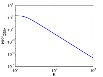
(a)   (b)

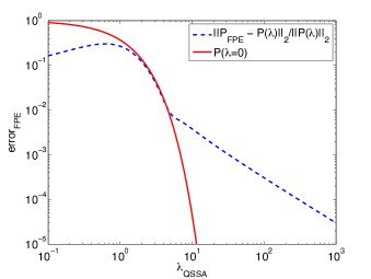
Fig. 1: (a) Plot of error $(\ref{eq:err})$, incurred by the QSSA for the system $\eqref{eq:lin}$ with reaction parameters given $k_{1}=k_{2}=1$ and $V=100$, as a function of $K$. (b) Blue plot shows error $(\ref{errorFPE})$ as a function of $\lambda_{\rm\scriptscriptstyle QSSA}$, for the system $(\ref{eq:eff})$. Red plot shows value of $\mathcal{P}(\lambda_{\rm\scriptscriptstyle QSSA})(0)$ as a function of $\lambda_{\rm\scriptscriptstyle QSSA}$.

The limitations of the stochastic quasi-steady-state approximation are looked at in detail in [28].

3.2 Diffusion Approximation Error

One of the sources of the error, common across all of three methods (CMA, NMA, QSSMA), is that we are approximating a Markov jump process which has a discrete state space (the non-negative integers), by a SDE with a continuous state space (the positive real numbers). To see the effect of this, let us consider the simple birth-death chemical system (15). The steady state solution to the CME for this system is given by the Poisson distribution (16). The closest approximation that we can get to this process with an SDE, is the chemical Langevin equation [14]. The corresponding stationary FPE for this system is

$$\frac{1}{2}\frac{\partial^{2}}{\partial s^{2}}\left(\Big{(}\bar{k}_{1}+\bar{k}_{2}s\Big{)}p(s)\right)-\frac{\partial}{\partial s}\left(\Big{(}\bar{k}_{1}-\bar{k}_{2}s\Big{)}p(s)\right)=0.$$ (18)

It can be explicitly solved to get [26].

$$p(s)=C\exp(-2s)(s+\lambda_{\rm\scriptscriptstyle QSSA})^{4\lambda_{\rm\scriptscriptstyle QSSA}-1},$$ (19)

where $C$ is determined by normalisation $\int p(s)\,\mbox{d}s=1.$ Here the integral is assumed to be taken over $s\geq 0$ (if we want to interpret $s$ as concentration) or $s\geq-\lambda_{\rm\scriptscriptstyle QSSA}$ (if we do not want to impose artificial boundary conditions at $s=0$). Considering more complicated systems, it is more natural to assume that the domain of the chemical Langevin equation is a complex plane [24].

Suppose we now wish to quantify the difference between probability distributions (16) and (19) as a function of $\lambda_{\rm\scriptscriptstyle QSSA}$. The first issue that we come across is that the solution of the steady-state CME is a probability mass function, and the solution to the steady-state FPE is a probability density function. However, we can simply integrate the probability density function over an interval of size one centered on each integer, to project this distribution onto a discrete state space with mass function $P_{\rm{FPE}}$ so that the two distributions can be compared:

$$P_{\rm{FPE}}(n)=\int^{n+1/2}_{n-1/2}P(s)\,\mbox{d}s.$$

Another issue is to specify the treatment of negative values of $s$. In our case we truncate the distribution for $s\geq 0$. We can then exactly calculate $P_{\rm{FPE}}$ to get

$$P_{\rm{FPE}}(n)=\frac{1}{\Gamma(4\lambda_{\rm\scriptscriptstyle QSSA})-\gamma(4\lambda_{\rm\scriptscriptstyle QSSA},2\lambda_{\rm\scriptscriptstyle QSSA})}\Big{(}\gamma(4\lambda_{\rm\scriptscriptstyle QSSA},2n+1+2\lambda_{\rm\scriptscriptstyle QSSA})-\gamma(4\lambda_{\rm\scriptscriptstyle QSSA},2n-1+2\lambda_{\rm\scriptscriptstyle QSSA})\Big{)},$$

where $\gamma(k,x)=\int_{0}^{x}z^{k-1}\exp(-z)\,\mbox{d}z$ denotes the lower incomplete gamma function and $\Gamma(k)=\int_{0}^{\infty}z^{k-1}\exp(-z)\,\mbox{d}z$ is the gamma function. Then we can consider the $l^{2}$ difference between these two distributions for a given value of $\lambda_{\rm\scriptscriptstyle QSSA}$,

$$\mbox{error}_{FPE}=\frac{\|P_{\rm{FPE}}-\mathcal{P}(\lambda_{\rm\scriptscriptstyle QSSA})\|_{2}}{\|\mathcal{P}(\lambda_{\rm\scriptscriptstyle QSSA})\|_{2}}=\sqrt{\sum_{n=0}^{\infty}\left(P_{\rm{FPE}}(n)-\frac{\lambda_{\rm\scriptscriptstyle QSSA}^{n}}{n!}\,\exp[-\lambda_{\rm\scriptscriptstyle QSSA}]\right)^{2}}.$$ (20)

Figure 1(b) shows how $\mbox{error}_{FPE}$ decays as $\lambda_{\rm\scriptscriptstyle QSSA}$ increases. The slightly odd sickle shaped error curve for small $\lambda_{\rm\scriptscriptstyle QSSA}$ is due to the probability mass of $\mathcal{P}(\lambda_{\rm\scriptscriptstyle QSSA})$ being peaked close to (or at) zero. In this region the diffusion approximation is very poor. To illustrate this, the value of $\mathcal{P}(\lambda_{\rm\scriptscriptstyle QSSA})$ at $s=0$, i.e. $\exp[-\lambda_{\rm\scriptscriptstyle QSSA}]$, is also plotted in Figure 1(b) (red curve). Once the peak of the probability mass has moved far enough away from zero, then the error is no longer dominated by being too close to zero, and decays inversely proportional to $\lambda_{\rm\scriptscriptstyle QSSA}$ (gradient of log-log plot is $-1.044$).

In the 2000 paper by Gillespie [14] on the chemical Langevin equation, a condition is put on the types of system which are well approximated by a diffusion. The probability of the system entering a state where the copy numbers of one or more of the chemical species in the state vector are close to zero must be small. Otherwise the approximation becomes poor. In the case of diffusion approximations of the slow variable(s) of a system, the trajectories must likewise stay away from regions of the state-space with low values of the slow variable(s). Further discussions and results regarding the accuracy of the chemical Langevin and Fokker-Planck equations can be found in [16].

3.3 Monte Carlo Error

The CMA and NMA both employ bursts of stochastic simulations to estimate the effective drift and diffusion of the slow variable. The main advantage of the QSSMA is that no such computation is required.

In the case of the CMA, as described in Section 2.1, the full system is simulated, including fast and slow reactions. The computed trajectory is constrained to a particular value of the slow variables, and so whenever a slow reaction occurs, the trajectory is projected back onto the same point on the slow manifold. The effective drift and diffusion at that point on the slow manifold are functions of statistics about the relative frequency of these slow reactions. As such, as given by the central limit theorem, the error in these estimations are mean zero and normally distributed, with variance proportional to $N_{S}^{-1}$, where $N_{S}$ is the number of slow reactions simulated during the estimation. Since it is necessary to simulate all of the fast and slow reactions in the system, depending on the difference in timescales this can be very costly. Since the ratio of occurrences of fast reactions to slow reactions is proportional to $K$, the cost of the estimation is $\mathcal{O}(K\,N_{S})$.

In comparison, the NMA, as described in Section 2.4, is only concerned with finding the average value of the fast variables through a Gillespie SSA simulation of only the fast variables. Therefore, the Monte Carlo error is again mean zero and normally distributed, with variance $N_{F}^{-1}$, where $N_{F}$ is the number of fast reactions simulated. Since we only simulate the fast reactions, the cost of the estimation is $\mathcal{O}(N_{F})$. Therefore, the cost of estimation for the CMA is approximately $K$-times that of the NMA for the same degree of accuracy.

3.4 Approximation of the solution of the stationary FPE

All three of the algorithms (CMA, NMA, QSSMA) also incur error through discretisation errors in the approximation of the solution to the steady-state FPE (6). The error of such an approximation is dependent on the method used, such as the adaptive finite element method used for three-dimensional chemical systems in [4]. In this paper we are mainly interested in the accuracy of the various methods for estimating the effective drift and diffusion functions, and as such we aim to simplify the methods for solving this PDE as much as possible. Therefore we will only consider systems with one-dimensional slow variables. The steady state equation corresponding to FPE (6) is then effectively an ordinary differential equation, and one which can be solved directly [14] to obtain

$$\mathcal{P}_{S}(s)=\frac{C}{D(s)}\exp\left(\int_{0}^{s}\frac{V(z)}{D(z)}\,\mbox{d}z\right),$$ (21)

where $C$ is the normalisation constant. With approximations of $V$ and $D$ over a range of values of $s$ (through implementation of the CMA, NMA or QSSMA), the integral in this expression can be evaluated using a standard quadrature routine (for instance the trapezoidal rule). The errors incurred here will be proportional to the grid size to some power, depending on the approximation method used.

3.5 Comparison of Sources of Error

Source of Error	CMA	NMA	QSSMA
Diffusion approximation	✔	✔	✔
QSSA	✖	✔	✔
Monte Carlo error	Cost - $\mathcal{O}(\mathcal{K}N_{S})$	Cost - $\mathcal{O}(N_{F})$	✖
PDE approximation	✔	✔	✔

Table 3: Table to summarise the sources of error of the three algorithms.

Table 3 summarises the analysis of the errors of the various methods that we have looked at in this section. Each method has advantages and disadvantages, depending on the type of system which a modeller wishes to apply the methods to. All of the methods use diffusion approximations, and as such, if the slow variables of the system of interest cannot be well approximated by a diffusion, then none of the proposed methods are suitable. If the QSSA does not hold for the system, then the CMA is the best choice. If it does hold, and the analytical solution for the effective propensities is available to us, then the QSSMA is the best choice, since it does not incur Monte Carlo, and is the least expensive of the three algorithms. Finally, if no such analytical solution is available, but the QSSA still holds, then the NMA is the best choice of algorithm, since it converges faster than the CMA.

Next, we apply the three methods to three different parameter regimes of the system given by (12). In each of the experiments, we set $k_{1}=k_{2}=1$ and $V=100$ and we vary $K$. We use $K=10$, $K=200$ and $K=10^{3}$. In each case, the CMA, NMA and the QSSMA are all applied to the system over the range of values $S=X_{1}+X_{2}\in[101,300]$. This range is chosen since the invariant distribution of the slow variable (14) is the Poisson random variable with intensity $\lambda_{0}=200+100/K$, and therefore the vast majority of the invariant density is contained with this region for all three parameter regimes. Furthermore, we implemented these algorithms on a computer with four cores, and to optimise the efficiency of parallelisation it was simplest to choose a domain with the number of states divisible by 4, hence the region starting at 101 as opposed to 100. For the CMA and the NMA, a range of different numbers of reactions were used in order to estimate the drift and diffusion parameters at each point, $N_{S},N_{F}\in\{10^{1},10^{2},\ldots,10^{9},10^{10}\}$. Each code was implemented in C, and optimised to the best of the authors’ ability, although faster codes are bound to be possible. The number of CPU cycles used was counted using the C time library. The CPU cycles used over all 4 cores were collated into a single number for each experiment.

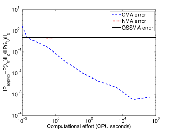
(a)   (b)

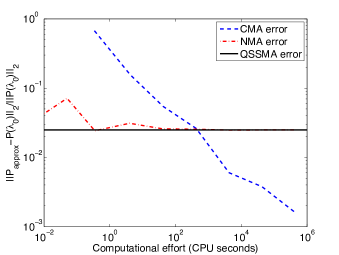
(c)

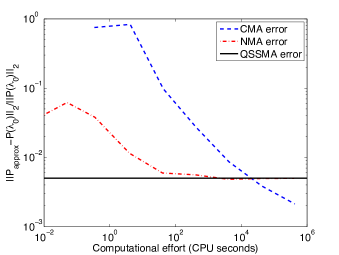
Fig. 2: (a) Error $(\ref{totalerror})$ of the CMA (blue), NMA (red) and the QSSMA (black) as the function of the computational effort for the chemical system $(\ref{eq:lin})$ with parameter values $k_{1}=k_{2}=1$, $V=100$ and $K=10$. For illustrative purposes the single value of the QSSMA error is plotted as a horizontal line. Actual computation time for the QSSMA is negligible. (b) As in panel (a), with $K=200.$ (c) As in panel (a), with $K=10^{3}.$ .

The results of these experiments are shown in Figure 2. Note that the results of the QSSMA and NMA are unaffected by a change in the value of $K$. In the case of the NMA, a change in the value of this variable simply scales time in computation of the fast subsystem, but does not affect the result. As such, only one run was necessary for these methods for the three different parameter regimes. The three plots for the NMA use the same simulations, but since the true distribution of the slow variable is affected by the change in $K$, the error plots differ across the three parameter regimes. In Figure 2 we plot the total relative error

$$\mbox{error}=\frac{\|P_{approx}-\mathcal{P}(\lambda_{0})\|_{2}}{\|\mathcal{P}(\lambda_{0})\|_{2}},$$ (22)

where $P_{approx}$ is the steady state distribution of the slow variable obtained by the corresponding method and $\mathcal{P}(\lambda_{0})$ is the exact solution given by (14). Figure 2(a), with $K=10$, denotes a parameter regime in which the QSSA produces a great deal of error. The NMA error quickly converges to the level seen in the QSSMA, but neither method can improve beyond this. The error seen from the CMA improves on both of these methods with relatively little computational effort. One might argue that the system is not actually a “true” multiscale system in this parameter regime, but the CMA still represents a good method for analysis of the dynamics of such a system, since its implementation can be parallelised in a way which scales linearly with the number of cores used.

Figure 2(c) shows a parameter regime which is highly multiscale. In this regime, the QSSA is far more reasonable, and as such we see vastly better performance from the NMA and QSSMA methods. However, eventually the CMA still has a higher accuracy than these two other approaches, although at not inconsiderable computational cost. In this case, the error incurred by the QSSA may be considered small enough that a modeller may be satisfied enough to use the QSSMA, whose costs are negligible. For more complex systems, the CME for the fast subsystem may not be exactly solvable, or even easily approximated, and in these cases the NMA would be an appropriate choice. If a more accurate approximation is required, once again the CMA could be used. In summary, even for simple system (12), with different parameter regimes, different methods could be considered to be preferable.

4 A bistable example

In this section, we will compare the presented methods for a multiscale chemical system which is bimodal, with trajectories switching between two highly favourable regions [5]:

$${\mbox{ \raise 1.13809pt\hbox{$X_{2}$}}}\;\mathop{\stackrel{{\scriptstyle\displaystyle\longrightarrow}}{{\longleftarrow}}}^{k_{1}}_{k_{2}}\;{\mbox{\raise 1.13809pt\hbox{$X_{1}+X_{2}$}}},\qquad{\mbox{ \raise 1.13809pt\hbox{$\emptyset$}}}\;\mathop{\stackrel{{\scriptstyle\displaystyle\longrightarrow}}{{\longleftarrow}}}^{k_{3}}_{k_{4}}\;{\mbox{\raise 1.13809pt\hbox{$X_{1}$}}},\qquad{\mbox{ \raise 1.13809pt\hbox{$X_{1}+X_{1}$}}}\;\mathop{\stackrel{{\scriptstyle\displaystyle\longrightarrow}}{{\longleftarrow}}}^{k_{5}}_{k_{6}}\;{\mbox{\raise 1.13809pt\hbox{$X_{2}$}}}.$$ (23)

One example of the parameter values for which this system is bistable for is given by:

$$k_{1}=32,\quad\frac{k_{2}}{V}=0.04,\quad k_{3}V=1475,\quad k_{4}=19.75,\quad\frac{k_{5}}{V}=10,\quad k_{6}=4000.$$ (24)

In this regime, reactions $R_{5}$ and $R_{6}$ (with rates $k_{5}$ and $k_{6}$ respectively) are occurring on a much faster time scale than the others. This can be seen in Figure 3, which shows the cumulative number of occurrences of each reaction in this system, simulated using the Gillespie SSA, given in Table 1. Both the species $X_{1}$ and $X_{2}$ are fast variables, since neither is invariant to the fast reactions. As in [5], we pick a slow variable which is invariant to reactions $R_{5}$ and $R_{6}$, $S=X_{1}+2X_{2}$. We now aim to compare the efficiency and accuracy of the CMA, NMA and QSSMA in approximating the stationary distribution in two different parameter regimes, with different spectral gaps between the fast and slow variables. This can be done by altering the values of rates $k_{5}$ and $k_{6}$.

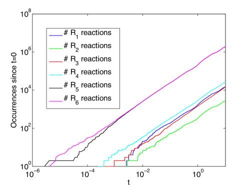
Fig. 3: Plot to show the frequency of the different reactions in the system (23) with parameters given by (24), computed using the Gillespie SSA, with initial condition ${\mathbf{X}}=[100,100]$.

One issue with using such a system, is that we cannot compute the analytical expression for the invariant density. Therefore, we compare with an accurate approximation of the invariant density.

4.1 Application of the NMA, QSSMA and CMA to reaction system (23)

For the NMA and the QSSMA, we assume that reactions $R_{5}$ and $R_{6}$ are occurring on a very fast time scale. Therefore we may assume that between reactions of other types (the slow reactions $R_{1}$-$R_{4}$), the subsystem involving only the fast reactions enters statistical equilibrium. In this case, we can reformulate (23) such that it is effectively a set of reactions which change the slow variable (reactions $R_{5}$ and $R_{6}$ are of course omitted as the slow variable $S=X_{1}+2X_{2}$ is invariant with respect to these reactions):

$${\mbox{ \raise 1.13809pt\hbox{$2S$}}}\;\mathop{\stackrel{{\scriptstyle\displaystyle\longrightarrow}}{{\longleftarrow}}}^{\widehat{k}_{1}}_{\widehat{k}_{2}}\;{\mbox{\raise 1.13809pt\hbox{$3S$}}},\qquad\mbox{\raise 1.13809pt\hbox{and}}\qquad{\mbox{ \raise 1.13809pt\hbox{$\emptyset$}}}\;\mathop{\stackrel{{\scriptstyle\displaystyle\longrightarrow}}{{\longleftarrow}}}^{\widehat{k}_{3}}_{\widehat{k}_{4}}\;{\mbox{\raise 1.13809pt\hbox{$S$}}}.$$ (25)

Next, we design the QSSMA by analytically computing the rates $\widehat{k}_{1}$, $\widehat{k}_{2}$ , $\widehat{k}_{3}$ and $\widehat{k}_{4}$.

To estimate the rates in (25) we must compute the average values of $X_{1}$ and $X_{2}$ for fixed value of $S=s$ in the fast subsystem:

$${\mbox{ \raise 1.13809pt\hbox{$X_{1}+X_{1}$}}}\;\mathop{\stackrel{{\scriptstyle\displaystyle\longrightarrow}}{{\longleftarrow}}}^{k_{5}}_{k_{6}}\;{\mbox{\raise 1.13809pt\hbox{$X_{2}$}}},\qquad X_{1}(0)+2X_{2}(0)=s.$$ (26)

As in [2], we approximate the mean values $\langle X_{1}\rangle$ and $\langle X_{2}\rangle$ of $X_{1}$ and $X_{2}$, respectively, by the solutions of the deterministic reaction rates equations. The authors showed that such an approximation is reasonably accurate for this particular fast subsystem (a reversible dimerisation reaction). Therefore, we need to solve the following system:

$$\frac{k_{5}}{V}\langle X_{1}\rangle^{2}=k_{6}\langle X_{2}\rangle,\qquad\langle X_{1}\rangle+2\langle X_{2}\rangle=s.$$

The nonnegative unique solution is given by:

$$\langle X_{1}\rangle=\frac{Vk_{6}}{4k_{5}}\left(\sqrt{1+8\frac{k_{5}}{Vk_{6}}s}-1\right)\qquad\mbox{and}\qquad\langle X_{2}\rangle=\frac{s-\langle X_{1}\rangle}{2}.$$ (27)

Then the effective propensity function of the slow reaction can be written as [2]:

$$\widehat{\alpha}_{1} = k_{1}\,\langle X_{2}\rangle,$$

$$\widehat{\alpha}_{2} = \frac{k_{2}\,s\,\langle X_{2}\rangle}{V}-\frac{2\,k_{2}\,\langle X_{2}\rangle^{2}}{V}+\frac{2\,k_{2}\,k_{6}\,\langle X_{2}\rangle}{8\,k_{5}\langle X_{2}\rangle-2\,k_{5}(2s+3)-k_{6}\,V}\;,$$ (28)

$$\widehat{\alpha}_{3} = k_{3}\,V,$$

$$\widehat{\alpha}_{4} = k_{4}\langle X_{1}\rangle=k_{4}\,\left(s-2\langle X_{2}\rangle\right).$$

More computational effort is required for this problem, since we need to compute $\langle X_{2}\rangle$ for each value of $S=s$ on the mesh. However, the computational effort is still negligible in comparison with the CMA or NMA. The biggest drawback with the QSSMA is the increase in mathematical complexity as the fast and slow systems themselves become more complicated. The more complexity there is, the more approximations need to be made in order to find the values of the effective propensities. The NMA simulations of the fast subsystem (26) in order to approximate the effective propensities (28), which are then fed into the Fokker-Planck equation for the slow sub-system. For the CMA simulations, we let $S=X_{1}+2X_{2}$ be the slow variable, and we let $X_{2}$ be the fast variable. For further details on how to apply the CMA to this system, see [5].

4.2 Numerical Results

In general, systems which have second (or through modelling assumptions, higher) order reactions cannot be solved exactly, although there are some special cases which can be tackled [15]. System (23) has second order reactions and hence we assume that the invariant distribution for the system cannot be solved analytically. As such, we are not able to compare the approximations arising from the three methods considered (CMA, QSSMA, NMA) to an exact solution. However, we can approximate the solution to the CME for this system, as we did in [5], by solving it on a truncated domain, assuming that the invariant distribution has zero probability mass everywhere outside this domain.

For the numerics that follow, we solve the CME on a truncated domain $\Omega=[0,10^{3}]\times[0,1.5\times 10^{3}]$. The CME on this domain gives us a sparse linear system, whose null space is exactly one dimensional. The corresponding null vector gives us, up to a constant of proportionality, our approximation of the solution of the CME. We normalise this vector, and then sum the invariant probability mass over states with the same value of the slow variable $S$. This procedure gives us the approximation of the invariant density of the slow variable which is plotted in Figure 4(a). Although this is only an approximation, it is a very accurate one. To demonstrate this, we compared the approximation of the solution $\mathcal{P}_{\Omega}$ of the steady-state CME on our chosen domain $\Omega=[0,10^{3}]\times[0,1.5\times 10^{3}]$ with an approximation $\mathcal{P}_{\omega}$ over a smaller domain, $\omega=[0,8.0\times 10^{2}]\times[0,1.25\times 10^{3}]$. The relative $l^{2}$ difference between these two approximations was $1.4571\times 10^{-11}$, indicating that any error in the approximation $\mathcal{P}_{\Omega}$ is highly unlikely to be of the order of magnitude of the errors seen in Figure 4(b), where we have used $\mathcal{P}_{\Omega}$ to approximate the error of multiscale methods.

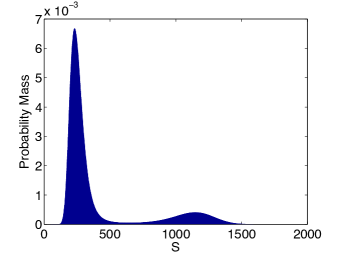
(a)   (b)

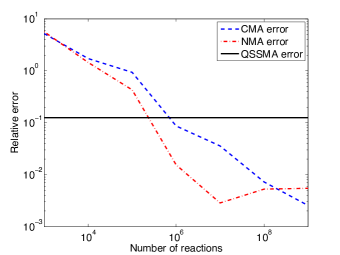
Fig. 4: (a) Approximation of the solution of the CME for the system (23) with parameters (24). The domain was truncated to $\Omega=[0,10^{3}]\times[0,1.5\times 10^{3}]$. (b) Approximation of the errors of the CMA, NMA and QSSMA for the system (23) with parameters (24). Error was estimated using the approximation of the solution of the CME shown in panel (a).

Figure 4(b) shows the error plots for the three methods for the system (23), using the approximation of the solution of the CME as the “exact” solution. The computational effort here is measured in terms of the numbers of simulated reactions. Since the computational cost for the two methods which use Monte Carlo simulations are dominated by the cost of producing two pseudo-random numbers for each iteration, this is a good estimate.

Unlike in the previous example, the distribution of the fast variables for a fixed value of the slow variables is not known analytically, and as such an approximation has been made, as was outlined in Section 4.1. As such, we no longer expect the NMA approximation to converge to the QSSMA approximation as in the last example. This can be seen in the error plot in Figure 4(b), where the error in the QSSMA approximation, which again had negligible cost to compute, is relatively high, with the NMA and CMA quickly outperforming it. The NMA slightly outperform the CMA at first, but appears to be unable to improve past a relative error of around $7\times 10^{-2}$. Note that this is 9 orders of magnitude bigger than the relative $l^{2}$ difference between $\mathcal{P}_{\Omega}$ and $\mathcal{P}_{\omega}$, and so is highly unlikely to be an artefact of the method we have used to approximate this error. As in the previous example, and as seen in [5], although the cost of the CMA is in general higher than the other methods, if a high precision solution is required, it is arguably the method of choice, as the error continues to decrease monotonically $\sim\mathcal{O}(\sqrt{N_{s}})$.

5 Discussion and conclusions

In this paper we have introduced two new methods for approximating the dynamics of slow variables in multiscale stochastic chemical networks, the NMA and QSSMA. These new methods combine ideas from the CMA [5], with ideas used in existing methods for speeding up the Gillespie SSA for multiscale systems [7, 2]. We then undertook a detailed numerical study of the different sources of error that these methods incur, for a simple chemical system for which we have an exact solution of the CME. Error is incurred due to the approximation of the dynamics by a diffusion process, Monte Carlo error in the approximation of the effective drift and diffusion terms, error due to application of the QSSA, and numerical error in approximation of the steady-state Fokker Planck equation, in various combinations. We then conducted another numerical study for a bistable chemical system, approximating the error by using an approximation of the solution to the CME for the system.

What we may surmise from this work, is that different methods, utilising different types of approximations, are appropriate for different types of system, or even in different parts of the parameter space of the same system. The methods in this paper differ from many others for stochastic fast/slow systems mainly in the approach of approximating the slow variables by a SDE. The majority of the other methods proposed in the literature use different ways of speeding up the Gillespie SSA for multiscale systems [23, 17, 7, 1]. In each, the full simulation of the fast species is replaced by some sort of approximation, so that an SSA-type algorithm, just for the slow species, may be implemented.

Many other approaches in the literature rely on a QSSA, including that taken by Rao and Arkin [23], Haseltine and Rawlings [17], E, Liu and Vanden-Eijnden [7] and Cao, Gillespie and Petzold [1]. All of these methods will incur the error that is seen in Figure 1(a). This error will be negligible for some systems, and significant for others, as we saw in Section 3.1, and in the difference between panels in Figure 2. One advantage of these methods over those that we have presented in this paper, is that they do not incur the continuous approximation error that we see in Figure 1(b) and discussed in Section 3.2. Diffusion approximation methods would not be appropriate if one wanted to analyse the dynamics of a slowly changing variable which has a low average copy number. For instance, in some gene regulatory network models, there are often two species, whose number sum to 1 in total, which represent whether a particular gene is “switched on” or “switched off”. Such a variable is clearly not a candidate for diffusion approximation. However, diffusion approximations have been used successfully for other variables in such systems [19]. The dynamics of that gene cannot themselves be approximated by a diffusion, but may be inferred from the state of other variables, which may be good candidates for such an approximation.

One big advantage of the diffusion approximation methods, is the ease with which the computational effort can be efficiently parallelised. This is a different approach to parallelisation than in the case of methods which calculate SSA trajectories. Several trajectories can be computed on different processors, but in order for the computed invariant distribution to be converged, either the initial positions of all of the trajectories must be sampled from the invariant distribution (which is unknown), or the trajectories must be run for enough time that each one is converged in distribution. On the other hand, the diffusion approximation approaches are almost embarrassingly parallelisable, with a subset of the states for which we wish to estimate the effective drift and diffusion being given to each processor. The solution of the Fokker-Planck equation is similarly parallelisable. This means that given enough computational resources, these algorithms can give us answers in a very short amount of time. Moreover, these approaches also allow us to consider adaptive mesh regimes [4], meaning that one can minimise the number of sites at which we are required to estimate the effective drift and diffusion values, while also controlling the global error incurred. This flexibility is not available in an SSA-type approach.

References

- [1] Y. Cao, D. Gillespie, and L. Petzold, Multiscale stochastic simulation algorithm with stochastic partial equilibrium assumption for chemically reacting systems, Journal of Computational Physics, 206 (2005), pp. 395–411.
- [2] , The slow-scale stochastic simulation algorithm, Journal of Chemical Physics, 122 (2005), p. 14116.
- [3] Y. Cao, H. Li, and L. Petzold, Efficient formulation of the stochastic simulation algorithm for chemically reacting systems, Journal of Chemical Physics, 121 (2004), pp. 4059–4067.
- [4] S. Cotter, T. Vejchodsky, and R. Erban, Adaptive finite element method assisted by stochastic simulation of chemical systems, SIAM Journal on Scientific Computing, 35 (2013), pp. B107–B131.
- [5] S. Cotter, K. Zygalakis, I. Kevrekidis, and R. Erban, A constrained approach to multiscale stochastic simulation of chemically reacting systems, Journal of Chemical Physics, 135 (2011), p. 094102.
- [6] M. Cucuringu and R. Erban, Detecting slow variables and their stationary distribution in high-dimensional stochastic dynamic data. in preparation, 2014.
- [7] W. E, D. Liu, and E. Vanden-Eijnden, Nested stochastic simulation algorithm for chemical kinetic systems with disparate rates, Journal of Chemical Physics, 123 (2005), p. 194107.
- [8] R. Erban, T. Frewen, X. Wang, T. Elston, R. Coifman, B. Nadler, and I. Kevrekidis, Variable-free exploration of stochastic models: a gene regulatory network example, Journal of Chemical Physics, 126 (2007), p. 155103.
- [9] R. Erban, I. Kevrekidis, D. Adalsteinsson, and T. Elston, Gene regulatory networks: A coarse-grained, equation-free approach to multiscale computation, Journal of Chemical Physics, 124 (2006), p. 084106.
- [10] R. Erban, I. Kevrekidis, and H. Othmer, An equation-free computational approach for extracting population-level behavior from individual-based models of biological dispersal, Physica D, 215 (2006), pp. 1–24.
- [11] R. Erban, S. J. Chapman, I. Kevrekidis, and T. Vejchodsky, Analysis of a stochastic chemical system close to a SNIPER bifurcation of its mean-field model, SIAM Journal on Applied Mathematics, 70 (2009), p. 984–1016.
- [12] M. Gibson and J. Bruck, Efficient exact stochastic simulation of chemical systems with many species and many channels, Journal of Physical Chemistry A, 104 (2000), pp. 1876–1889.
- [13] D. Gillespie, Exact stochastic simulation of coupled chemical reactions, Journal of Physical Chemistry, 81 (1977), pp. 2340–2361.
- [14] , The chemical Langevin equation, Journal of Chemical Physics, 113 (2000), pp. 297–306.
- [15] R. Grima, D. Schmidt, and T. Newman, Steady-state fluctuations of a genetic feedback loop: an exact solution, Journal of Chemical Physics, 137 (2012), p. 035104.
- [16] R. Grima, P. Thomas, and A. Straube, How accurate are the chemical Langevin and Fokker-Planck equations?, Journal of Chemical Physics, 135 (2011), p. 084103.
- [17] E. Haseltine and J. Rawlings, Approximate simulation of coupled fast and slow reactions for stochastic chemical kinetics, Journal of Chemical Physics, 117 (2002), pp. 6959–6969.
- [18] T. Jahnke and W. Huisinga, Solving the chemical master equation for monomolecular reaction systems analytically, Journal of Mathematical Biology, 54 (2007), pp. 1–26.
- [19] T. Kepler and T. Elston, Stochasticity in transcriptional regulation: Origins, consequences and mathematical representations, Biophysical Journal, 81 (2001), pp. 3116–3136.
- [20] G. Klingbeil, R. Erban, M. Giles, and P. Maini, STOCHSIMGPU: Parallel stochastic simulation for the Systems Biology Toolbox 2 for MATLAB, Bioinformatics, 27 (2011), pp. 1170–1171.
- [21] S. Liao, T. Vejchodsky and R. Erban, Tensor methods for parameter estimation and bifurcation analysis of stochastic reaction networks, submitted to Journal of the Royal Society Interface (2014).
- [22] Z. Liu, Y. Pu, F. Li, C. Shaffer, S. Hoops, J. Tyson, and Y. Cao, Hybrid modeling and simulation of stochastic effects on progression through the eukaryotic cell cycle, Journal of Chemical Physics, 136 (2012), p. 034105.
- [23] C. Rao and A. Arkin, Stochastic chemical kinetics and the quasi-steady-state assumption: application to the Gillespie algorithm, Journal of Chemical Physics, 118 (2003), pp. 4999–5010.
- [24] D. Schnoerr, G. Sanguinetti, and R. Grima, The complex chemical Langevin equation, Journal of Chemical Physics, 141 (2014), p. 024103.
- [25] A. Singer, R. Erban, I. Kevrekidis, and R. Coifman, Detecting the slow manifold by anisotropic diffusion maps, Proceedings of the National Academy of Sciences USA, 106 (2009), pp. 16090–16095.
- [26] P. Sjöberg, P. Lötstedt, and J. Elf, Fokker-Planck approximation of the master equation in molecular biology, Computing and Visualization in Science, 12 (2009), pp. 37–50.
- [27] P. Thomas, R. Grima, and A. Straube, Rigorous elimination of fast stochastic variables from the linear noise approximation using projection operators, Physical Review E, 86 (2012), p. 041110.
- [28] P. Thomas, A. Straube, and R. Grima, Limitations of the stochastic quasi-steady-state approximation in open biochemical reaction networks, Journal of Chemical Physics, 135 (2011), p. 181103.
- [29] , The slow-scale linear noise approximation: an accurate, reduced stochastic description of biochemical networks under timescale separation conditions, BMC Systems Biology, 6 (2012), p. 39.
- [30] X. Xue, Computational methods for chemical systems with fast and slow dynamics, Master’s thesis, University of Oxford, 2012.