Watersheds in disordered media

Abstract

What is the best way to divide a rugged landscape? Since ancient times, watersheds separating adjacent water systems that flow, for example, toward different seas, have been used to delimit boundaries. Interestingly, serious and even tense border disputes between countries have relied on the subtle geometrical properties of these tortuous lines. For instance, slight and even anthropogenic modifications of landscapes can produce large changes in a watershed, and the effects can be highly nonlocal. Although the watershed concept arises naturally in geomorphology, where it plays a fundamental role in water management, landslide, and flood prevention, it also has important applications in seemingly unrelated fields such as image processing and medicine. Despite the far-reaching consequences of the scaling properties on watershed-related hydrological and political issues, it was only recently that a more profound and revealing connection has been disclosed between the concept of watershed and statistical physics of disordered systems. This review initially surveys the origin and definition of a watershed line in a geomorphological framework to subsequently introduce its basic geometrical and physical properties. Results on statistical properties of watersheds obtained from artificial model landscapes generated with long-range correlations are presented and shown to be in good qualitative and quantitative agreement with real landscapes.

I Introduction

Although both start in the mountains of Switzerland, the Rhine and Rhone rivers diverge while flowing towards different seas. While the Rhine empties into the North Sea, the Rhone drains into the Mediterranean. Similarly, all over the world one finds rivers with close sources but distant mouths. For example, the Colorado and the Rio Grande even open towards different oceans. When looking at a landscape, how to identify the regions draining towards one side or the other? When rain falls or snow melts on a landscape, the dynamics of the surface water is determined by the topography of the landscape. Water flows downhill and overpasses small mounds by forming lakes which eventually overspill. A drainage basin is then defined as the region where water flows towards the same outlet. Its shape and extension strongly depend on the topography. The line separating two adjacent basins is the watershed line, which typically wanders along the mountain crests Gregory and Walling (1973).

Since watersheds provide information about the dynamics of surface water, they play a fundamental role in water management Vörösmarty et al. (1998); Kwarteng et al. (2000); Sarangi and Bhattacharya (2005), landslides Dhakal and Sidle (2004); Pradhan et al. (2006); Lazzari et al. (2006); Lee and Lin (2006), and flood prevention Lee and Lin (2006); Burlando et al. (1994); Yang et al. (2007). Watersheds are also of relevance in the political context they have been used to demarcate borders between countries such as the one between Argentina and Chile United Nations (2006). Thus, the understanding of their statistical properties and resilience to changes in the topography of the landscape are two important questions that we will review here. In general, for every landscape, several outlets can be defined, each one with a corresponding drainage basin. Sets of small drainage basins eventually drain towards the same outlet forming a even larger basin. Such hierarchy results in a larger number of watersheds. However, without loss of generality, the study of watershed lines can be simplified by splitting the landscape into only two large basins, each one draining towards opposite boundaries. Figure 1 shows how this watershed can be identified by flooding the landscape from the valleys (see supplemental video). Two sinks are initially defined (the lower-left and upper-right boundaries in the example). While flooding the landscape, each time two lakes (A and B) draining towards opposite sinks are about to connect, one imposes a physical barrier between the two. In the end, the watershed line is the line formed by the barriers that separate these two lakes.

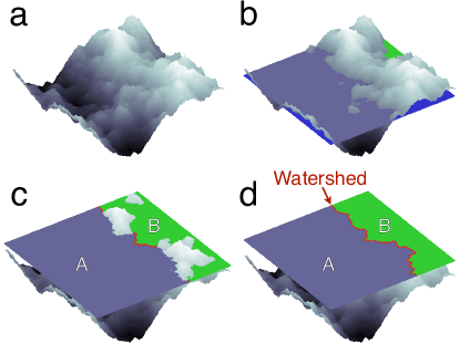
Figure 1: Watershed dividing a landscape into two parts. The landscape (a) is flooded from the valleys such that all regions lower than a certain height are covered with water (b). As the water level rises, lakes merge under the constraint that no lake can connect two predefined opposite boundaries of the landscape (c). In this example, we have taken the lower-left and the upper-right boundaries. Thus, a watershed line emerges separating the two final lakes (d). These lakes (A and B) are the drainage basins of this landscape. 

The concept of watersheds is also of interest in other fields like, e.g., in medical image processing Dixon (1979). There, computed tomography scans need to be segmented to identify different tissues. The pictures are discretized into pixels and a number is assigned to each one of them according to the intensity. The segmentation procedure consists in clustering neighboring pixels following the order of increasing intensity gradient, splitting the image into different parts (tissues). The equivalent to the watershed line corresponds to the line separating two different tissues Yan et al. (2006); Patil and Patilkulkarani (2009).

It was recently shown that watersheds can be described in the context of percolation theory in terms of bridges and cutting bond models Schrenk et al. (2012a), with numerical evidence that they are Schramm-Loewer Evolution (SLE) curves in the continuum limit Daryaei et al. (2012). This association explains why watersheds on uncorrelated landscapes as well as other statistical physics models, such as, optimal path cracks Andrade Jr. et al. (2009, 2011); Oliveira et al. (2011), fuse networks Moreira et al. (2012), and loopless percolation Schrenk et al. (2012a), belong to the same universality class of optimal paths in strongly disordered media.

II The landscape

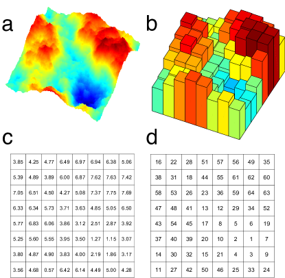
Figure 2: The process of generating a ranked surface. The landscape in (a) is coarse-grained to the low-resolution system of $8\times 8$ cells shown in (b), and then represented as a discretized map of local heights, as depicted in (c). By ranking these heights in crescent order, one obtains the ranked surface in (d). In fact, the landscape shown in (a) is a high resolution synthetic map obtained from a fractional Brownian motion simulation based on the Fourier filtering method (see Sec. VII). 

The motion of surface water is defined by the topology of the landscape, usually characterized by the spatial distribution of heights. Although this distribution is a continuous function for real landscapes, it is typically coarse-grained and represented as a digital elevation map (DEM) of regular cells (e.g., a square lattice of sites or bonds) to which average heights can be associated. This process is exemplarily shown in Figs. 2(a)-(c). In fact, modern procedures of analyzing real landscapes numerically process Grayscale Digital Images where the gray intensity of each pixel is transformed into a height, resulting in a DEM. As such, discretized maps have been useful to delimit spatial boundaries in a wide range of problems, from tracing watersheds and river networks in landscapes Stark (1991); Maritan et al. (1996); Manna and Subramanian (1996); Knecht et al. (2012); Baek and Kim (2012) to the identification of cancerous cells in human tissues Yan et al. (2006); Ikedo et al. (2007), and the study of spatial competition in multispecies ecosystems Kerr et al. (2006); Mathiesen et al. (2011).

To study watersheds theoretically one can generate artificial landscapes. Starting with a regular lattice, a numerical value is randomly assigned to each element, corresponding to its average height. If these values are spatially correlated, a correlated artificial landscape is obtained. Otherwise, the landscape is called an uncorrelated artificial landscape. Natural landscapes are characterized by long-range correlations Pastor-Satorras and Rothman (1998). In Sec. VII we will review how to generate correlated artificial landscapes and their main properties.

The DEM can be further simplified by mapping them onto ranked surfaces, where every element (site or bond) has a unique rank associated with its corresponding value Schrenk et al. (2012a). A ranked surface can be defined in the following way. Given a two-dimensional discretized map of size $L\times L$, one generates a list containing the heights of its elements (sites or bonds) in crescent order, and then replaces the numerical values in the original map by their corresponding (integer) ranks. As depicted in Fig. 2(d), the result is a ranked surface.

III How to determine the watershed

Traditional cartographic methods for basin delineation have relied on manual estimation from iso-elevation lines. Instead, modern procedures are now based upon automatic processing of images as the ones obtained from satellites Farr et al. (2007); Vincent and Soille (1991). These images are typically coarse-grained into discretized maps with each cell $i$ having a height $h_{i}$ as explained in Sec. II. A recently proposed algorithm to identify watersheds that became rather popular consists in the flooding procedure described in Fig. 1 Vincent and Soille (1991), considering two sinks such as, for example, two opposite boundaries. Cells in the discretized map are ranked according to their height, which leads to a ranked surface, and are sequentially occupied, following the rank, from the lowest to the highest. Neighboring occupied cells are then connected and considered part of the same drainage basin, except when during this process their connection would promote the agglomeration of the two basins draining towards different sinks. In this case, their connection is avoided, since they should belong to different basins. The edge between them is part of the watershed and, at the end, the set of such edges forms one single watershed line that splits the landscape into two drainage basins (see Fig. 1).

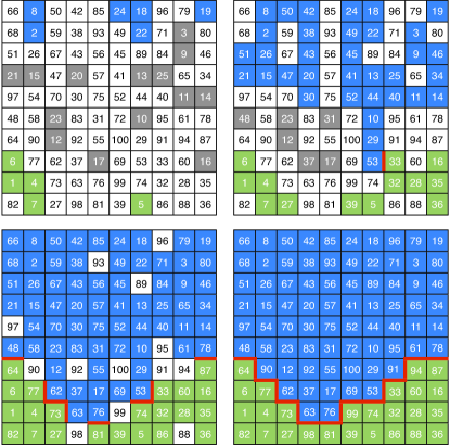
Figure 3: Flooding algorithm to determine the watershed. Two sinks are considered: the top row and the bottom one. Cells in the discretized map are occupied following the rank, from the lowest to the highest. Neighboring occupied cells are considered connected and part of the same basin (gray cells). The basins connected to the top row (blue) correspond to the ones draining towards the top sink. Similarly, the ones connected to the bottom row (green) drain towards the bottom sink (upper-left panel). If two neighbors of the next cell in the rank belong to basins of different sinks, the edges in contact with the cells are marked as elements of the watershed (red-thick edges). The process proceeds iteratively until all cells are flooded (bottom panels). At the end (bottom-right panel), the watershed splits the discretized map into two basins (blue and green). 

The flooding procedure implies visiting every cell in the discretized map. Fehr and co-workers Fehr et al. (2009) have devised a more efficient identification algorithm where only a fractal subset needs to be visited. The algorithm is based on Invasion Percolation (IP) Wilkinson and Willemsen (1983) and consists in the following procedure. One initially defines two sinks (for example, the bottom and top rows of the discretized map) and considers that the (non-invaded) cell with the lowest height on the perimeter of the (already) invaded region is the next cell to be invaded. If when starting from one cell a sink is invaded, the initial cell and the entire invaded region is considered to belong to the catchment basin of that sink. Consider that the invasion is initially started from the cell in the bottom-right corner. Since this cell is part of the basin of the bottom sink, the invaded region has only one cell. One proceeds with a new invasion from the next cell upwards (cell $35$ in Fig. 4) and a new invasion cluster is grown until a sink is reached. Sequentially, all other cells are considered in the same way. The watershed is then identified as the line splitting the landscape into two catchment basins. The efficiency is significantly improved if, once the first cell-edge belonging to the watershed has been identified, the exploration continues from the cells in the neighborhood of this edge (see Fig. 4). Thus, instead of visiting all cells, only a subset of $N_{\mathrm{exp}}$ cells needs to be explored. For uncorrelated random landscapes, the size of this subset scales with the linear size of the DEM $L$ as $N_{\mathrm{exp}}\sim L^{D}$, with $D=1.8\pm 0.1$ Fehr et al. (2009).

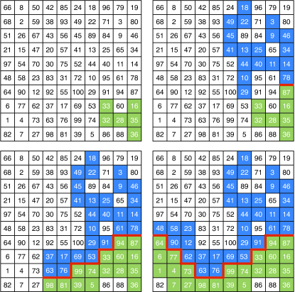
Figure 4: Algorithm based on Invasion Percolation. As in Fig. 3, two sinks are considered: the top and the bottom rows. One starts from the bottom-right corner (cell $36$). Since this site is in the bottom row, it is already part of the bottom sink (green). Proceeding upwards, following the most right column, the next unexplored cell is considered (cell $35$). The basin to which this cell belongs grows by adding the smallest-height cell on its perimeter, until one sink is reached (cells $16$, $28$, $32$, and $33$ in the upper-left panel, reaching $36$). Proceeding further to the top, the cell $87$ is added to the (green) basin (connecting to $16$). When the cell $78$ is considered and the corresponding basin grown, a new (blue) basin is found draining towards the upper sink (upper-right panel). The cell-edge between cell $87$ and $78$ is considered part of the watershed (red-thick edge). Proceeding by iteratively identifying the basin of the cells in the neighborhood of the watershed edges, the full watershed is identified (bottom panels). Since the same initial ranked surface is considered, the final watershed is equal to the one obtained in Fig. 3. 

IV Fractal dimension

Table 1: Fractal dimension of watersheds for natural landscapes obtained from satellite imagery Farr et al. (2007) in Ref. Fehr et al. (2011a). The values for the Alps and Himalayas are from Ref. Fehr et al. (2009). The error bars are of the order of $2\%$.

Landscape	$d_{f}$
Alpes	1.10
Europe	1.10
Rocky Mountains	1.11
Himalayas	1.11
Kongo	1.11
Andes	1.12
Appalachians	1.12
Brazil	1.12
Germany	1.14
Big Lakes	1.15

Breyer and Snow Breyer and Snow (1992) have studied $12$ basins in the United States and concluded that their watershed lines are self-similar objects Mandelbrot (1967, 1983). A self-similar structure is characterized by its fractal dimension $d_{f}$, which is defined here through the scaling of the number $M$ of edges belonging to the watershed with the linear size $L$ of the discretized map,

$$M\sim L^{d_{f}}\,\,.$$ (1)

They obtained fractal dimensions in the range $1.05-1.12$. Fehr and co-workers Fehr et al. (2009), with the method described in Sec. III confirmed this self-similar behavior over more than three orders of magnitude and measured the fractal dimension for watersheds in several real landscapes, as summarized in Tab. 1.

For uncorrelated artificial landscapes the watershed fractal dimension has been estimated to be $d_{f}=1.2168\pm 0.0005$ Cieplak et al. (1994); Fehr et al. (2009, 2012). This value has drawn considerable attention since it was also found in several other physical models such as optimal paths in strong disorder and optimal path cracks Porto et al. (1997); Buldyrev et al. (2004); Andrade Jr. et al. (2009, 2011); Oliveira et al. (2011), bridge percolation Cieplak et al. (1994, 1996); Schrenk et al. (2012a), and the surface of explosive percolation clusters Araújo and Herrmann (2010); Schrenk et al. (2011). The conjecture that all these models might belong to the same universality class has opened a broad range of possible implications and applications of the properties of watersheds. As discussed in Ref. Schrenk et al. (2012a), the relation between most of such models can be established when they are described within the framework of ranked surfaces (see also Sec. II).

V Watersheds in three and higher dimensions

Up to now, we have focused on the watershed line that divides the landscape into drainage basins for water on the surface. However, in reality, water also penetrates the soil and flows underground. Thus, the concept of watersheds and ranked surfaces can be extended to three dimensions. The soil can be described as a porous medium consisting of a network of pores connected through channels. When a fluid penetrates through this medium, a threshold pressure $p_{k}$ can be defined for each channel $k$ such that the channel can only be invaded when $p\geq p_{k}$, where $p$ is the fluid pressure. In general, a channel $k$ is closed when $p_{k}>p$, and open otherwise. This system can be mapped into a three dimensional ranked volume, where the lattice elements are the channels and the rank is defined by the increasing order of the threshold pressure. The sequence in the rank corresponds to the order of channel openings when the fluid pressure is quasistatically raised from zero. Analogously to the ranked surfaces, one can split the space in two regions, draining towards opposite boundaries.

The watershed in three dimensions is a surface of fractal dimension $d_{f}=2.487\pm 0.003$ Fehr et al. (2012). An example for a simple-cubic ranked volume is shown in Fig. 5. In general, for lattices of size $L^{d}$, where $d$ is the spatial dimension, the watershed blocks connectivity from one side to the other. Thus, the watershed fractal dimension must follow $d-1\leq d_{f}\leq d$, i.e., with increasing dimension $d_{f}$ also increases Schrenk et al. (2012a).

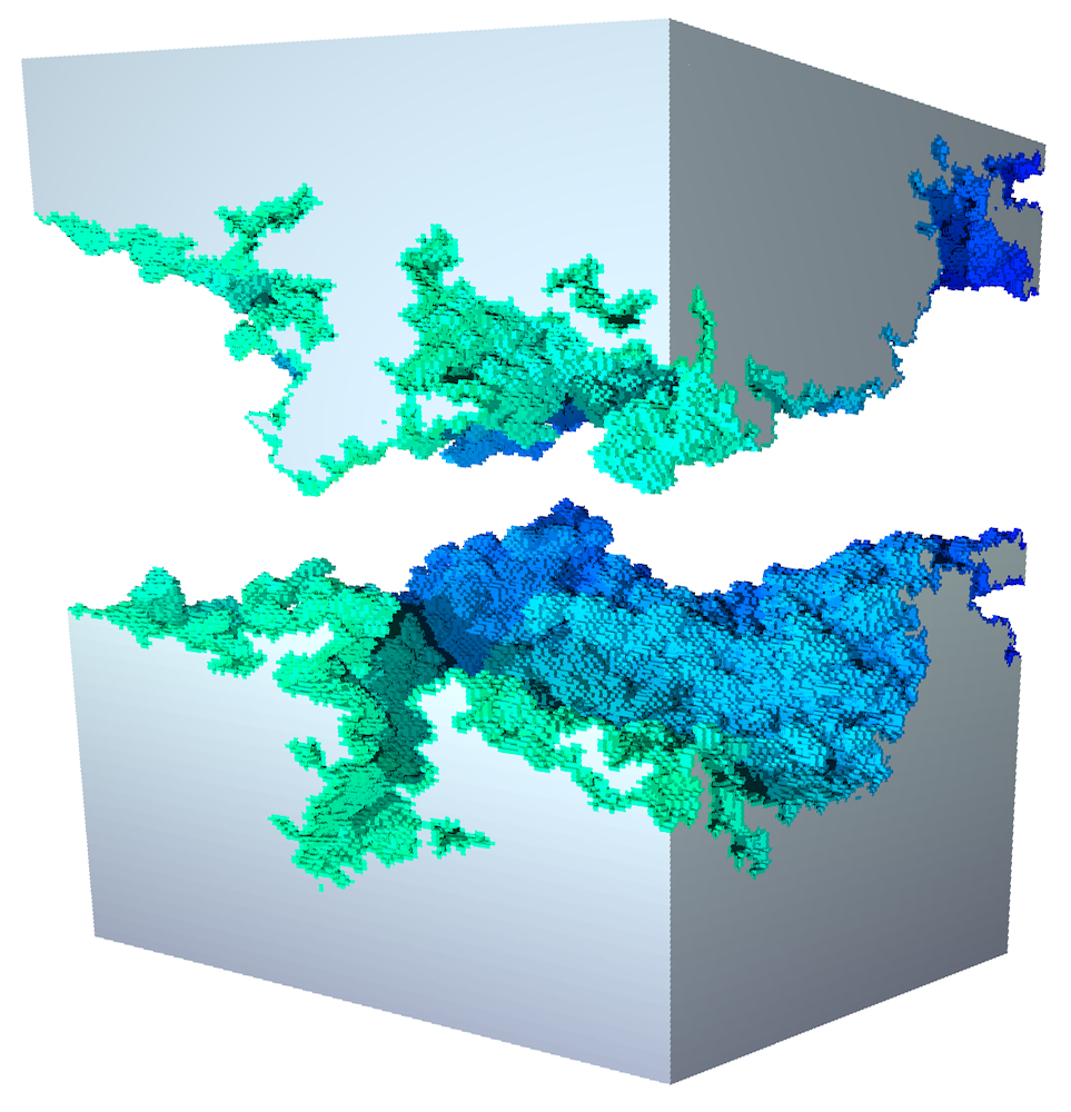
Figure 5: Watershed in three dimensions. Example of a watershed for an uncorrelated three-dimensional space, namely, a simple-cubic lattice of $128^{3}$ sites. To obtain the watershed, sites are sequentially occupied under the constraint that groups of connected sites in contact with the top boundary cannot merge with the ones connected to the bottom boundary. In three dimensions, the fractal dimension is $d_{f}=2.487\pm 0.003$ Fehr et al. (2012). 

VI Impact of perturbation on watersheds

The stability of watersheds is also a subject of interest. For example, changes in the watershed might affect the sediment supply of rivers Douglass and Schmeeckle (2007). Also, the understanding of the temporal evolution of drainage networks provides valuable insight into the biodiversity between basins Bishop (1995). Geographers and geomorphologists have found that the evolution of watersheds is typically driven by local changes of the landscape Burridge et al. (2007). These events can be triggered by various mechanisms like erosion Garcia-Castellanos et al. (2009); Linkevičienė (2009); Bishop (1995), natural damming Lee and Lin (2006), tectonic motion Garcia-Castellanos et al. (2003); Dorsey and Roering (2006); Lock et al. (2006), as well as volcanic activity Beranek et al. (2006). Although rare, these local events can have a huge impact on the hydrological system Attal et al. (2008); Garcia-Castellanos et al. (2009); Linkevičienė (2009); Burridge et al. (2007). For example, it was shown that a local height change of less than two meters at a location close to the Kashabowie Provincial Park, some kilometers North of the US-Canadian border, can trigger a displacement in the watershed such that the area enclosed by the original and the new watersheds is about $3730~{}\mbox{km}^{2}$ Fehr et al. (2011b).

The stability of watersheds is also relevant in the political context. For example, Chile and Argentina share a common border with more than $5000$ kilometers, which was the source of a long dispute between these countries United Nations (2006). A treaty established this border as being the watershed between the Atlantic and Pacific Oceans for several segments. In $1902$, the Argentinian Francisco Moreno contributed significantly to elucidate the technical basis for dispute. He proved that during the quarternary glaciations, the watershed line changed. In particular, several Patagonian lakes currently draining to the Pacific Ocean were in fact originally part of the Atlantic Ocean basin. Consequently, he argued, instead of belonging to Chile they should be awarded to Argentina.

Douglas and Schmeeckle Douglass and Schmeeckle (2007) have performed fifteen table top experiments to study the mechanisms of drainage rearrangements. In spite of being diverse, the mechanisms triggering the evolution of watersheds are all modifications of the topography Bishop (1995); Lee and Lin (2006); Garcia-Castellanos et al. (2003). In that perspective, the effect of such events can be investigated by applying small local perturbations to natural and artificial landscapes and analyzing the changes in the watershed Fehr et al. (2011b, a). Specifically, one starts with a discretized landscape and computes the original watershed. A local event is then induced by changing the height of a site $k$ $h_{k}\rightarrow h_{k}+\Delta$, where $\Delta$ is the perturbation strength, and the new watershed is identified. The impact of perturbations on watersheds in two and three dimensions will be discussed in the following.

VI.1 Impact of perturbations in two dimensions

Fehr and co-workers Fehr et al. (2011b) have normalized the perturbation strength by the height difference between the highest and lowest height of the landscape. For each landscape, they have sequentially perturbed every site of the corresponding discretized map, such that each perturbed landscape differs from the original only in one single site. The effect of those perturbations affecting the watershed has been quantified by the properties of the region enclosed by the original and the new watersheds. For that region, they have measured its area, corresponding to the number of sites, $N_{s}$, in the discretized map and the distance $R$ between its original and new outlets, defined as the points where water escapes from this region. Note that, there are only two outlets involved in this procedure: one related to the original landscape and the other to the new one. Since $\Delta$ is strictly positive, the outlet in the new landscape corresponds always to the perturbed site $k$.

Scale-free behavior has been found for the distribution $P(N_{s})$ of the number of enclosed sites $N_{s}$, the probability distribution $P(R)$ of the distance $R$ between outlets, and the dependence of the average $\langle N_{s}\rangle$ on $R$ Fehr et al. (2011b, a). Specifically,

$$P(N_{s}) \sim N_{s}^{-\beta},$$ (2a)

$$P(R) \sim R^{-\rho},$$ (2b)

$$\langle N_{s}\rangle \sim R^{\sigma},$$ (2c)

where the measured exponents are summarized in Tab. 2. The power-law decay (2b) and the relation (2c) imply that a localized perturbation can have a large impact on the shape of the watershed even at very large distances, hence having a non-local effect. Additionally, the analysis of the fraction of perturbed sites affecting the watershed revealed a power-law scaling with the strength $\Delta$. This finding supports the conclusion that changes in the watershed can be even triggered by anthropological small perturbations Fehr et al. (2011b).

Table 2: Exponents for the impact of perturbations on watersheds, calculated for uncorrelated artificial landscapes in two and three dimensions, from Refs. Stauffer and Aharony (1994); Fehr et al. (2011b, a, 2012).

Exponent	Uncorrelated landscapes
$d$	2		3
$d_{f}$	1.2168$\pm$	0.0005	2.487$\pm$	0.003
$\beta$	1.16$\pm$	0.03	1.31$\pm$	0.05
$\rho$	2.21$\pm$	0.01	3.2$\pm$	0.2
$\sigma$	2		2.45$\pm$	0.05
$\alpha^{*}$	1.39$\pm$	0.03	1.4$\pm$	0.1

For the region enclosed by the original and the new watersheds, an invasion percolation (IP) cluster can be obtained by imposing a pressure drop between the outlet in the new watershed and the one in the original one, always invading along the steepest descent of the entire cluster perimeter. The size distribution $P(M_{\mathrm{IP}}|R)$ of these clusters, for each fixed distance $R$ between outlets, has been shown to scale as,

$$P(M_{\mathrm{IP}}|R)\sim M_{IP}^{-(1+\alpha^{*})}\ \ ,$$ (3)

where $\alpha^{*}\approx 1.39$. This exponent corresponds to the one found for the size distribution of point-to-point IP-clusters Araújo et al. (2005). In that process, invasion clusters are obtained in a random medium by invading from one point to another at a certain distance. By contrast, in the watershed case the invasion is always started from the outlet on the new watershed. This difference between starting at any point or in the outlet justifies the additional factor of unity in the scaling (Eq. (3)), since the probabilities need to be rescaled by the size of the IP-cluster Fehr et al. (2011b).

VI.2 Impact of perturbations in three dimensions

The impact of perturbations on watersheds has been also analyzed in three dimensions Fehr et al. (2011a). Similar to 2D, a perturbation is induced by changing the value of a site $k$, $h_{k}\rightarrow h_{k}+\Delta$, where $\Delta$ is the perturbation strength. The number of sites $N_{s}$ enclosed by the original and new watersheds corresponds to a volume. Power-law scaling in terms of Eqs. (2a)-(2c) has also been observed with the exponents summarized in Tab. 2. The value of $\alpha^{*}$ is similar to the one found in two dimensions. According to Lee Lee (2009), the size distribution of the point-to-point IP-cluster is independent on the dimensionality of the system. Therefore, the numerical agreement between $\alpha^{*}$ for different spatial dimensions supports the relation with invasion percolation.

VII Watersheds on long-range correlated landscapes

Results discussed heretofore were obtained on random uncorrelated landscapes. However real landscapes are characterized by spatial long-range correlated height distributions. Numerically, such distributions can be generated from fractional Brownian motion (fBm) Mandelbrot (1967); Peitgen and Saupe (1988), using the Fourier filtering method Fehr et al. (2011b); Morais et al. (2011); Sahimi (1994); Sahimi and Mukhopadhyay (1996); Makse et al. (1996); Oliveira et al. (2011); Prakash et al. (1992); Kikkinides and Burganos (1999); Stanley et al. (1999); Makse et al. (2000); Araújo et al. (2002, 2003); Du et al. (1996). This method allows to control the nature and the strength of correlations, which are characterized by the Hurst exponent $H$. The uncorrelated distribution of heights is solely obtained for $H=-d/2$, i.e., $H=-1$ and $H=-3/2$ in two and three dimensions, respectively. A detailed description of this method can be found, e.g., in Ref. Oliveira et al. (2011); Peitgen and Saupe (1988).

Fehr et al. Fehr et al. (2011b, a) used fractional Brownian motion (fBm) on a square lattice Lauritsen et al. (1993) to incorporate long-range correlations controlled by the Hurst exponent $H$. They calculated how the fractal dimension decreases with the Hurst exponent and found good quantitative agreement with the exponents obtained for natural landscapes, typically with $0.3<H<0.5$, which is the known range of Hurst exponents for real landscapes on length scales larger than 1 km (see Ref. Pastor-Satorras and Rothman (1998) and references therein). They also obtained $\alpha$, $\beta$ and $\rho$ for several values of $H$, observing that both $\beta$ and $\rho$ increase with $H$, finding also good quantitative agreement. Thus, their model provides a complete quantitative description of the effects observed on natural landscapes.

VIII Final Remarks

Here we solely discussed cases with one watershed, but the same theoretical framework can be straightforwardly extended to tackle other space partition problems. For example, the identification of the entire set of watersheds of a landscape with multiple outlets helps identifying the catchment areas contributing to each river or reservoir Mamede et al. (2012). A systematic study of disordered media with multiple outlets is still missing. Examples of open questions are: How does the distribution of catchment basins or the number of triplets (points where two watersheds meet) depend on the number of outlets? And, how does the statistics of perturbations change in the presence of triplets? The division of a volume into several parts is also a problem of practical interest in the extraction of resources from porous soils Schrenk et al. (2012b). Studies of such systems have mainly considered uncorrelated disordered media. The role of long-range correlation there is still an open problem.

References

- Gregory and Walling (1973) K. J. Gregory and D. E. Walling, Drainage basin form and process: A geomorphological approach (Edward Arnold, London, 1973).
- Vörösmarty et al. (1998) C. J. Vörösmarty, C. A. Federer, and A. L. Schloss, J. Hydrol. 207, 147 (1998).
- Kwarteng et al. (2000) A. Y. Kwarteng, M. N. Viswanathan, M. N. Al-Senafy, and T. Rashid, J. Arid. Environ. 46, 137 (2000).
- Sarangi and Bhattacharya (2005) A. Sarangi and A. K. Bhattacharya, Agr. Water Manage. 78, 195 (2005).
- Dhakal and Sidle (2004) A. S. Dhakal and R. C. Sidle, Hydrol. Process. 18, 757 (2004).
- Pradhan et al. (2006) B. Pradhan, R. P. Singh, and M. F. Buchroithner, Adv. Space Res. 37, 698 (2006).
- Lazzari et al. (2006) M. Lazzari, E. Geraldi, V. Lapenna, and A. Loperte, Landslides 3, 275 (2006).
- Lee and Lin (2006) K. T. Lee and Y.-T. Lin, J. Am. Water Resour. As. 42, 1615 (2006).
- Burlando et al. (1994) P. Burlando, M. Mancini, and R. Rosso, IFIP Trans. B 16, 91 (1994).
- Yang et al. (2007) D. Yang, Y. Zhao, R. Armstrong, D. Robinson, and M.-J. Brodzik, J. Geophys. Res. 112, F02S22 (2007).
- United Nations (2006) United Nations, “The Cordillera of the Andes boundary case (Argentina, Chile), 20 November 1902,” (2006), http://untreaty.un.org/cod/riaa/cases/volIX/29-49.pdf.
- Dixon (1979) J. K. Dixon, IEEE T. Syst. Man Cyb. 9, 617 (1979).
- Yan et al. (2006) J. Yan, B. Zhao, L. Wang, A. Zelenetz, and L. H. Schwartz, Med. Phys. 33, 2452 (2006).
- Patil and Patilkulkarani (2009) C. M. Patil and S. Patilkulkarani, in IEEE Proceedings of ARTCom 2009 (2009) p. 796.
- Schrenk et al. (2012a) K. J. Schrenk, N. A. M. Araújo, J. S. Andrade Jr., and H. J. Herrmann, Sci. Rep. 2, 348 (2012a).
- Daryaei et al. (2012) E. Daryaei, N. A. M. Araújo, K. J. Schrenk, S. Rouhani, and H. J. Herrmann, Phys. Rev. Lett. 109, 218701 (2012).
- Andrade Jr. et al. (2009) J. S. Andrade Jr., E. A. Oliveira, A. A. Moreira, and H. J. Herrmann, Phys. Rev. Lett. 103, 225503 (2009).
- Andrade Jr. et al. (2011) J. S. Andrade Jr., S. D. S. Reis, E. A. Oliveira, E. Fehr, and H. J. Herrmann, Comput. Sci. Eng. 13, 74 (2011).
- Oliveira et al. (2011) E. A. Oliveira, K. J. Schrenk, N. A. M. Araújo, H. J. Herrmann, and J. S. Andrade Jr., Phys. Rev. E 83, 046113 (2011).
- Moreira et al. (2012) A. A. Moreira, C. L. N. Oliveira, A. Hansen, N. A. M. Araújo, H. J. Herrmann, and J. S. Andrade Jr., Phys. Rev. Lett. 109, 255701 (2012).
- Stark (1991) C. P. Stark, Nature 352, 423 (1991).
- Maritan et al. (1996) A. Maritan, F. Colaiori, A. Flammini, M. Cieplak, and J. R. Banavar, Science 272, 984 (1996).
- Manna and Subramanian (1996) S. S. Manna and B. Subramanian, Phys. Rev. Lett. 76, 3460 (1996).
- Knecht et al. (2012) C. L. Knecht, W. Trump, D. ben-Avraham, and R. M. Ziff, Phys. Rev. Lett. 108, 045703 (2012).
- Baek and Kim (2012) S. K. Baek and B. J. Kim, Phys. Rev. E 85, 032103 (2012).
- Ikedo et al. (2007) Y. Ikedo, D. Fukuoka, T. Hara, H. Fujita, E. Takada, T. Endo, and T. Morita, Med. Phys. 34, 4378 (2007).
- Kerr et al. (2006) B. Kerr, C. Neuhauser, B. J. M. Bohannan, and A. M. Dean, Nature 442, 75 (2006).
- Mathiesen et al. (2011) J. Mathiesen, N. Mitarai, K. Sneppen, and A. Trusina, Phys. Rev. Lett. 107, 188101 (2011).
- Pastor-Satorras and Rothman (1998) R. Pastor-Satorras and D. H. Rothman, Phys. Rev. Lett. 80, 4349 (1998).
- Farr et al. (2007) T. G. Farr, P. A. Rosen, E. Caro, R. Crippen, R. Duren, S. Hensley, M. Kobrick, M. Paller, E. Rodriguez, L. Roth, D. Seal, S. Shaffer, J. Shimada, J. Umland, M. Werner, M. Oskin, D. Burbank, and D. Alsdorf, Rev. Geophys. 45, RG2004 (2007).
- Vincent and Soille (1991) L. Vincent and P. Soille, IEEE T. Pattern Anal. 13, 583 (1991).
- Fehr et al. (2009) E. Fehr, J. S. Andrade Jr., S. D. da Cunha, L. R. da Silva, H. J. Herrmann, D. Kadau, C. F. Moukarzel, and E. A. Oliveira, J. Stat. Mech. , P09007 (2009).
- Wilkinson and Willemsen (1983) D. Wilkinson and J. F. Willemsen, J. Phys. A 16, 3365 (1983).
- Fehr et al. (2011a) E. Fehr, D. Kadau, N. A. M. Araújo, J. S. Andrade Jr., and H. J. Herrmann, Phys. Rev. E 84, 036116 (2011a).
- Breyer and Snow (1992) S. P. Breyer and R. S. Snow, Geomorphology 5, 143 (1992).
- Mandelbrot (1967) B. Mandelbrot, Science 156, 636 (1967).
- Mandelbrot (1983) B. B. Mandelbrot, The Fractal Geometry of Nature (Freeman, New York, 1983).
- Cieplak et al. (1994) M. Cieplak, A. Maritan, and J. R. Banavar, Phys. Rev. Lett. 72, 2320 (1994).
- Fehr et al. (2012) E. Fehr, K. J. Schrenk, N. A. M. Araújo, D. Kadau, P. Grassberger, J. S. Andrade Jr., and H. J. Herrmann, Phys. Rev. E 86, 011117 (2012).
- Porto et al. (1997) M. Porto, S. Havlin, S. Schwarzer, and A. Bunde, Phys. Rev. Lett. 79, 4060 (1997).
- Buldyrev et al. (2004) S. V. Buldyrev, S. Havlin, E. López, and H. E. Stanley, Phys. Rev. E 70, 035102(R) (2004).
- Cieplak et al. (1996) M. Cieplak, A. Maritan, and J. R. Banavar, Phys. Rev. Lett. 76, 3754 (1996).
- Araújo and Herrmann (2010) N. A. M. Araújo and H. J. Herrmann, Phys. Rev. Lett. 105, 035701 (2010).
- Schrenk et al. (2011) K. J. Schrenk, N. A. M. Araújo, and H. J. Herrmann, Phys. Rev. E 84, 041136 (2011).
- Douglass and Schmeeckle (2007) J. Douglass and M. Schmeeckle, Geomorphology 84, 22 (2007).
- Bishop (1995) P. Bishop, Prog. Phys. Geog. 19, 449 (1995).
- Burridge et al. (2007) C. P. Burridge, D. Craw, and J. M. Waters, Mol. Ecol. 16, 1883 (2007).
- Garcia-Castellanos et al. (2009) D. Garcia-Castellanos, F. Estrada, I. Jiménez-Munt, C. Gorini, M. Fernàndez, J. Vergés, and R. De Vicente, Nature 462, 778 (2009).
- Linkevičienė (2009) R. Linkevičienė, Holocene 19, 1233 (2009).
- Garcia-Castellanos et al. (2003) D. Garcia-Castellanos, J. Vergés, J. Gaspar-Escribano, and S. Cloetingh, J. Geophys. Res. 108, 2347 (2003).
- Dorsey and Roering (2006) R. J. Dorsey and J. J. Roering, Geomorphology 73, 16 (2006).
- Lock et al. (2006) J. Lock, H. Kelsey, K. Furlong, and A. Woolace, Geol. Soc. Am. Bull. 118, 1232 (2006).
- Beranek et al. (2006) L. P. Beranek, P. K. Link, and C. M. Fanning, Geol. Soc. Am. Bull. 118, 1027 (2006).
- Attal et al. (2008) M. Attal, G. E. Tucker, A. C. Whittaker, P. A. Cowie, and G. P. Roberts, J. Geophys. Res. 113, F03013 (2008).
- Fehr et al. (2011b) E. Fehr, D. Kadau, J. S. Andrade Jr., and H. J. Herrmann, Phys. Rev. Lett. 106, 048501 (2011b).
- Stauffer and Aharony (1994) D. Stauffer and A. Aharony, Introduction to Percolation Theory, 2nd ed. (Taylor and Francis, London, 1994).
- Araújo et al. (2005) A. D. Araújo, T. F. Vasconcelos, A. A. Moreira, L. S. Lucena, and J. S. Andrade Jr., Phys. Rev. E 72, 041404 (2005).
- Lee (2009) S. B. Lee, Physica A 388, 2271 (2009).
- Peitgen and Saupe (1988) H.-O. Peitgen and D. Saupe, eds., The Science of Fractal Images (Springer, New York, 1988).
- Morais et al. (2011) P. A. Morais, E. A. Oliveira, N. A. M. Araújo, H. J. Herrmann, and J. S. Andrade Jr., Phys. Rev. E 84, 016102 (2011).
- Sahimi (1994) M. Sahimi, J. Phys. I France 4, 1263 (1994).
- Sahimi and Mukhopadhyay (1996) M. Sahimi and S. Mukhopadhyay, Phys. Rev. E 54, 3870 (1996).
- Makse et al. (1996) H. A. Makse, S. Havlin, M. Schwartz, and H. E. Stanley, Phys. Rev. E 53, 5445 (1996).
- Prakash et al. (1992) S. Prakash, S. Havlin, M. Schwartz, and H. E. Stanley, Phys. Rev. A 46, R1724 (1992).
- Kikkinides and Burganos (1999) E. S. Kikkinides and V. N. Burganos, Phys. Rev. E 59, 7185 (1999).
- Stanley et al. (1999) H. E. Stanley, J. S. Andrade Jr., S. Havlin, H. A. Makse, and B. Suki, Physica A 266, 5 (1999).
- Makse et al. (2000) H. A. Makse, J. S. Andrade Jr., and H. E. Stanley, Phys. Rev. E 61, 583 (2000).
- Araújo et al. (2002) A. D. Araújo, A. A. Moreira, H. A. Makse, H. E. Stanley, and J. S. Andrade Jr., Phys. Rev. E 66, 046304 (2002).
- Araújo et al. (2003) A. D. Araújo, A. A. Moreira, R. N. Costa Filho, and J. S. Andrade Jr., Phys. Rev. E 67, 027102 (2003).
- Du et al. (1996) C. Du, C. Satik, and Y. C. Yortsos, AIChE Journal 42, 2392 (1996).
- Lauritsen et al. (1993) K. B. Lauritsen, M. Sahimi, and H. J. Herrmann, Phys. Rev. E 48, 1272 (1993).
- Mamede et al. (2012) G. L. Mamede, N. A. M. Araújo, C. M. Schneider, J. C. de Araújo, and H. J. Herrmann, Proc. Natl. Acad. Sci. USA 109, 7191 (2012).
- Schrenk et al. (2012b) K. J. Schrenk, N. A. M. Araújo, and H. J. Herrmann, Sci. Rep. 2, 751 (2012b).