Puoko-nui: A Flexible High-speed Photometric System

Abstract

We describe a portable CCD-based instrumentation system designed to efficiently undertake high time precision fast photometry. The key components of the system are (1) an externally triggered commercial frame-transfer CCD, (2) a custom GPS-derived time source, and (3) flexible software for both instrument control and online analysis/display. Two working instruments that implement this design are described. The New Zealand based instrument employs a Princeton Instruments (PI) 1k$\times$1k CCD and has been used with the 1 m telescope at Mt. John University Observatory, while the other uses a newer 1k$\times$1k electron-multiplying CCD supplied by PI and is based at the University of Texas at Austin. We include some recent observations that illustrate the capabilities of the instruments.

1 Introduction

There are a number of interesting astronomical phenomena with timescales between tens of milliseconds and tens of minutes. These include g-mode pulsations in white dwarfs (e.g. Winget & Kepler, 2008; Fontaine & Brassard, 2008; Althaus et al., 2010) and p-mode oscillations in the hot subdwarf B stars (e.g. Fontaine et al., 2006). Both these classes of objects exhibit photometric variability with periods $\sim 10^{2}$ – $10^{3}$ s.

Other phenomena are the eclipsing short period double-degenerate systems (e.g. Hermes et al., 2012), $\sim 10^{1}-10^{2}$ s; planetary occultations, $\sim 10^{-1}$ s; and optical pulsars (e.g. Cocke et al., 1969), $\sim 10^{-2}$ s.

Our primary interests are with the pulsating white dwarfs, which are unstable to g-mode pulsation in several instability strips that are a function of the surface temperature and the dominant chemical atmospheric constituent. These stars are also predicted to be unstable to p-mode pulsations with periods $\sim 1$ s, but any consequent luminosity variations have so far never been observed (e.g. Silvotti et al., 2011; Kilkenny et al., 2014).

An important aspect of high-speed photometry is accurate timing. The pulsating white dwarfs, in particular, can have complicated pulsation spectra with closely spaced frequencies that can require tens of hours of continuous observation to properly resolve. This requires a clock that remains sufficiently stable over an extended period during an acquisition run, and also between successive days to allow multiple acquisition runs to be combined for analysis. Furthermore, groups like the Whole Earth Telescope (Nather et al., 1990) coordinate observations from different observatories around the globe in order to minimize data gaps, thus extending the problem to multiple geographically distributed clocks.

This was a challenge in earlier decades, but has now been essentially solved by sourcing time from the Global Positioning System (GPS) network. GPS disciplined clocks which provide accurate time to $\mu$s or better are readily available from several commercial manufacturers. The challenge in designing an instrument is how best to integrate this time information into the overall system. A common approach (e.g, Dhillon et al., 2007) is to operate the CCD asynchronously and record the GPS-determined time at the start and/or end of an exposure. An alternative approach is to use a GPS-disciplined clock to trigger CCD readouts at known times. We use this approach in our Puoko-nui instruments.

The increasing availability of electron-multiplying frame-transfer CCDs makes it feasible to take photon-noise limited exposures at high frame-rates. It is therefore important that the timing resolution is high enough so as to not artificially limit the capabilities of the instrument.

2 Instrument Overview

The basic design for our system evolved from an earlier instrument, Argos (Nather & Mukadam, 2004), which pioneered efficient CCD photometry of pulsating white dwarfs. This development marked a significant departure from the multi-channel photomultiplier-based instruments (e.g. Kleinman et al., 1996; Sullivan, 2000) that were previously used for these observations.

The key components of the Argos design philosophy were to use a commercial frame-transfer CCD in combination with GPS-derived timing signals in order to accomplish accurate time-series photometry as fast as 1 Hz, and essentially free from dead-time (readout) losses. An online display of the incoming light curves to guide observers was also included. One time-series CCD photometer (Agile) that has successfully evolved from the Argos design has already been described in the literature (Mukadam et al., 2011).

Argos had several limitations which made it unsuitable to directly copy when creating Puoko-nui (which means “big eye” in NZ Maori). A major problem was the concentration of all the required control functions along with the acquisition and analysis software in one PC. Although this configuration had the apparent advantage of simplicity, it created difficulties when changes were required. In addition, largely as a result of the camera manufacturer providing an interface via inadequately described binary code, the software required a specific version of the Linux operating system kernel that did not operate well with newer hardware.

In the Puoko-nui design we have separated the timing and control functions from the acquisition and analysis operations by developing a microcontroller-based unit that operates independently of the acquisition PC. This unit uses GPS signals to maintain accurate time and output synchronised CCD control signals; it communicates with the acquisition PC via USB. We have also developed more flexible software packages for acquisition and analysis. This increased flexibility made it relatively simple to extend support to a newer and somewhat different CCD camera from the same manufacturer, which required the acquisition and analysis software to run in a Microsoft Windows environment. We will discuss both instrument flavours in this paper.

The original Puoko-nui (South) photometer, pictured in Fig. 1, is based in NZ and has been operating in its current form since mid 2011; publications that include observational data acquired with this instrument are listed in Section 3. The second instrument (Puoko-nui North) is based at the University of Texas at Austin and has been operational since late 2012.

Fig. 2 gives a schematic overview of the main components of the Puoko-nui system, and they are explained in more detail in the following sections.

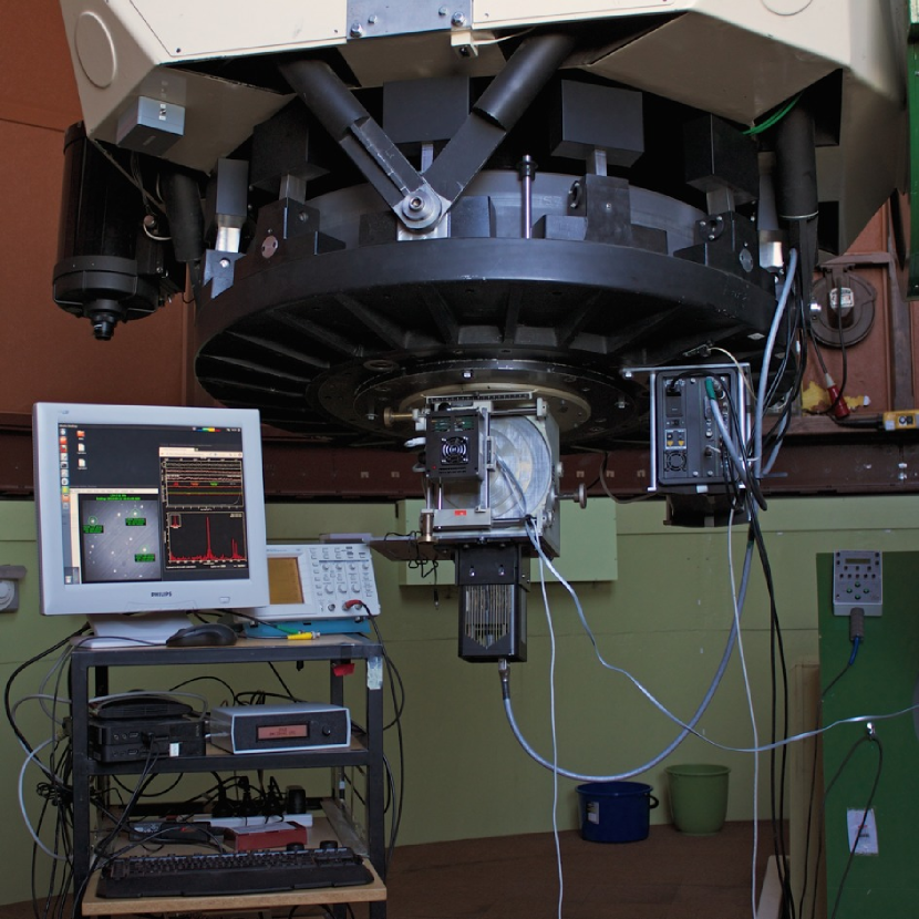
Figure 1: The complete Puoko-nui South instrument mounted on the 1 m McLellan telescope at Mt John University Observatory, Lake Tekapo, New Zealand.

Figure 2: A block diagram depicting the main components of Puoko-nui South. Puoko-nui North mounts the science camera directly on the telescope, and auto-guides using the science frames.

2.1 Science Cameras

Both instruments use Princeton Instruments (PI) camera systems, containing E2V back-illuminated $1024\times 1024$ px frame-transfer CCDs with $13\times 13\,\mu$m pixels. Puoko-nui South employs a PI MicroMax camera with a USB data interface, while Puoko-nui North uses a PI ProEM camera with a gigabit ethernet interface. The detailed specifications for the two cameras are shown in Table 1.

The back-illumination of a CCD improves the quantum efficiency at shorter wavelengths, which is particularly useful when observing the hot white dwarfs. The use of a frame-transfer CCD further improves the efficiency by essentially eliminating readout deadtimes.

The readout of a CCD (as compared with e.g. the CMOS sensor used more commonly in consumer cameras) is a serial process, in which the charge from each pixel is clocked across the sensor towards a single (or small number of) readout registers. The readout process can take several seconds or more, during which a standard CCD must be shuttered from incident light in order to prevent the creation of additional extraneous charge in the pixels.

Frame-transfer CCDs contain twice the area of a regular sensor, with half of it permanently masked as a readout storage region. The accumulated charge is shifted to this region at the end of an exposure, allowing the time-consuming final readout phase to occur in parallel with the next exposure.

This rapid shifting of charge between exposures removes the need for a mechanical shutter, allowing the instrument to operate without moving parts. When operated this way, there will be a small amount of image smearing caused by photons impacting the CCD while the charge is being shifted into the storage region, but given the very short transfer times this effect may only be non-negligible at the shortest exposures. For the ProEM camera a full frame transfer takes only $\sim 1\,$ms, while it is $\sim 16\,$ms for the MicroMax camera.

The ProEM camera also features an electron-multiplication (EM) readout port (Mackay et al., 2001), which allows a pre-amplification of up to $1000\times$ to be applied to the integrated image before it is measured. This can allow the signal to overcome the readout noise (which is often the dominant noise source), making it practical to acquire frames with a greater time resolution. The EM readout mode also features faster readout rates, which correspondingly reduces the minimum exposure length; 0.12 s for the fastest full-frame readout at 10 MHz, compared with 1.2 s for the MicroMax at 1 MHz. In both cases, the readout time can be further reduced by reading out a smaller sub-area of the CCD.

Both cameras are thermo-electrically cooled, with the MicroMax camera operating at $-50^{\circ}$C, and the ProEM at $-55^{\circ}$C. The ProEM includes an additional heat exchanger that can be connected to a liquid cooling system for increased cooling efficiency.

The key feature that makes these cameras suitable for our purposes is that they allow the frame transfer and subsequent readout to be triggered externally. The internal oscillators used within the cameras were measured to be stable to $\sim 1$ part in $10^{5}$, which is excellent for a single exposure, but this accumulates to a total drift of as much as 50 ms per hour. The external trigger enables the exposure timing to be controlled by an external clock, which can be disciplined against a reference time standard (e.g. GPS) to provide consistent exposure triggers that remain aligned to the UTC-second boundary over arbitrarily long run lengths.

Table 1: A comparison of the science cameras in the two instruments. The noise measurement for the ProEM’s Electron Multiplication mode is given for $1000\times$ avalanche gain.

Parameter	Puoko-nui South	Puoko-nui North
PI Model	MicroMax	ProEM
Connectivity	USB 2.0	Gigabit Ethernet
CCD Type	E2V Back Illuminated	E2V Back Illuminated EMCCD
Active Area (px)	$1024\times 1024$	$1024\times 1024$
Mode	Frame Transfer	Frame Transfer
Pixel Size ($\mu$m)	13	13
Vertical Clock Time ($\mu$s / row)	15.2	1
ADC Bit Depth (bits)	16	16
Full Well Depth (ke-)	110	120
Dark Current (e-/ px / s)	0.2	0.01
Shutter	None	Electro-mechanical
Software API	PVCAM (32-bit Linux)	PICAM (64-bit Windows)
Readout Type	Low Noise	Low Noise	EM
Readout Rates (MHz)	0.1, 1	0.1, 1, 5	5, 10
Noise (e- rms)	5.0 – 13	3.2 – 13	0.03 – 0.04
Gain (e-/ ADU)	1.0 – 4.5	0.7 – 3.4	2.1 – 11.4
EM Gain	–	–	1 – 1000

2.2 Timing hardware

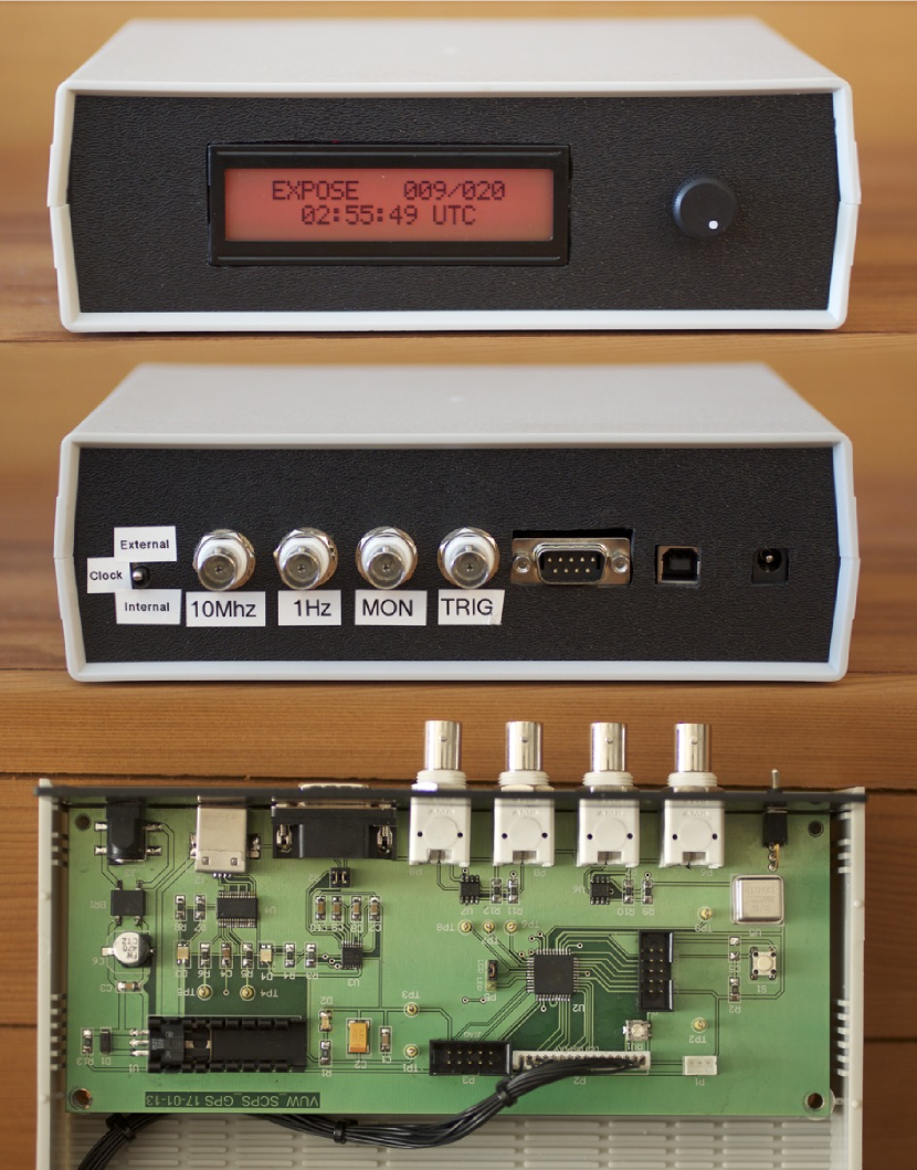
Figure 3: The Puoko-nui timer unit is built around a stand-alone microcontroller, allowing it to operate independently during an acquisition sequence. Time and exposure information is sent to the Acquisition PC via a standard USB 2.0 connection.

Precise exposure timing is provided by a custom timer/counter unit, which is pictured in Fig. 3. The unit is built around an Atmel AVR microcontroller, and communicates with the acquisition PC via USB. The USB connectivity, paired with the USB/Ethernet cameras allows the instrument to be controlled using a standard PC laptop or small-form-factor ‘netbook’ computer without requiring any additional hardware.

The primary function of the timer unit is to process time signals from an external GPS disciplined clock (currently supporting the Trimble Thunderbolt and a legacy Magellan OEM receiver) to manage the exposure timing. The GPS time signals are provided in the form of 1 Hz and 10 MHz pulse trains via coaxial cables, and a RS232 serial stream of ASCII-coded absolute time information.

The unit features two timing modes, which operate by counting pulses on either the 10 MHz pulse input (high-resolution mode) or the 1 Hz pulse input (low resolution mode). In both modes the unit counts pulses up to the desired exposure length, and then outputs a frame-transfer trigger to the camera. The GPS time associated with each trigger is sent to the acquisition PC to be written into the frame header data.

Externally triggering the individual frame transfers simplifies the process of integrating precise timing with a commercial camera system. This separation of timing and acquisition was an important factor in the rapid development of Puoko-nui North, and allows for additional camera systems to be supported in the future with only minimal changes.

The two timing modes are compared in Table 2. The high-resolution mode is preferred, as it contains additional checks for potential timing discrepancies. The low-resolution mode remains available as a fallback for acquiring exposures longer than 65 seconds, or when operating using our Magellan GPS receiver, which does not conveniently provide a 10 MHz signal in its current form.

Table 2: The timer unit features two operating modes. The high-resolution mode supports trigger periods as short as $1\,$ms, but in practice the camera readout speed limits exposures to $>5\,$ms and telescope-size currently limits useful white-dwarf observations to $>1\,$s for Puoko-nui South.

Mode	High-res.	Low-res.
Exp. range	1 ms – 65.5 s	1 s – 18.2 h
Exp. resolution	1 ms	1 s
Trigger delay	$<1\,\mu$s	18 ms
Trigger instability	$<10\,\mu$s	$<10\,\mu$s
Required inputs	1 Hz, 10 MHz, RS232	1 Hz, RS232

The trigger delay figure in Table 2 was obtained by comparing the 1 Hz GPS pulse train against the generated trigger pulses using an oscilloscope. The camera response time between the trigger and frame transfer beginning was similarly measured at $<1\,\mu$s. In the case of the high-resolution mode, the phase of the trigger pulse can be advanced or delayed in order to minimize the difference against the UTC-second aligned 1 Hz input. We have explicitly verified the absolute timing accuracy of Puoko-nui South to better than 20 ms by imaging the time display of the older three-channel photometer master clock, which was set using an independent GPS receiver. Observations of the Crab Pular using Puoko-nui North (see Section 3) further verifies the timing accuracy to within a few ms, limited by the precision of our software reduction pipeline. The trigger instability figure is calculated based on the possibility of a hardware interrupt being delayed while another is serviced, which may introduce a delay of up to 100 clock cycles (10 $\mu$s). This situation is rare, and the measured jitter usually remains below 1 $\mu$s.

The shortest possible exposure time is limited by the camera readout rate (which in itself depends on factors such as the readout window parameters), but the exposure time will be limited in most situations by the accumulation of sufficient photons from the faint targets. For maximum flexibility, we wanted to ensure that the timing system did not impose any additional constraints, particularly for a portable instrument that may have the opportunity to be used on telescopes larger than the original design specified.

A secondary function of the timer is to monitor the camera readout status via a logic output. This is necessary to work around a bug in the closed source camera firmware and pvcam library for the MicroMax camera: terminating an exposure sequence mid-readout can corrupt the internal state of the ‘black-box’ software and cause subsequent exposure sequences to be corrupted. The software API does not allow the camera status to be queried, and so a hardware work-around was implemented using the timer to monitor the programmable logic output on the camera to determine its current state.

The USB connection between the timer and acquisition PC is configured to provide a 9600 baud serial communication channel. We have chosen this limited data rate (USB allows speeds up to 3 Mbaud) in part to match the GPS receivers. This allows the timer (when operating in its ‘relay’ mode) to transparently forward data between the GPS receiver and acquisition PC so that other software on the PC can interact with it. The limited data rate is sufficient for normal operation with exposure lengths greater than 0.1 s. Shorter exposures are supported by reducing the number of trigger timestamps sent to the acquisition PC (sending only 1 in N exposures, where N is chosen to keep the data transfer similar to 0.5 s exposures). The intermediate timestamp values are synthesised by the acquisition PC.

2.3 Acquisition software

The acquisition and control software is written primarily in the C programming language and is portable across 32 and 64 bit versions of Linux, Windows and Mac OS X. In practice, the availability of (proprietary) camera drivers currently restricts operation to 32 bit Linux (using Ubuntu 12.04) for Puoko-nui South, and 64-bit Windows 7 for Puoko-nui North.

The acquisition software performs three main tasks: configuring the acquisition parameters, matching frame data with timestamps during acquisition, and notifying the user of the current hardware status. The acquisition software is divided into a number of concurrent threads that communicate asynchronously. The components and main information flow are shown in Fig. 4.

Fig. 5 shows the run configuration parameters and the customisable information fields that are saved into the frame headers. The camera and timer are configured with these parameters when the user starts an acquisition run, and the software then becomes responsive to incoming frame data and trigger timestamps.

Frame data from the camera and trigger timestamps from the timer are received from their respective hardware interfaces, and passed to a processing thread. The processing thread performs a basic validation check to ensure that the frame being associated with each timestamp is correct (the time that the frame was received minus the readout time should match the trigger timestamp to within a small margin of error), and then saves the frame and associated metadata to disk as a compressed FITS image.

The Puoko-nui South instrument can acquire arbitrarily long acquisition sequences, limited only by disk space. The faster readout rates supported by Puoko-nui North can result in the situation where the data rate from the camera exceeds the disk write rate; frames will be buffered in memory until the backlog of frames have been purged to disk. This could be improved by installing a faster solid-state hard disk, however this is unnecessary for the $\sim$ second exposures used for our primary white dwarf targets.

The most recently acquired frame is displayed using the SAOImage DS9 software, and can be overlaid with information on one or more selected comparison stars. This information is calculated on a per-frame basis independently of the online reduction, and can be used for auto-guiding the telescope (see Section 2.5).

Figure 4: A block diagram depicting the key software threads in the Puoko-nui acquisition software.

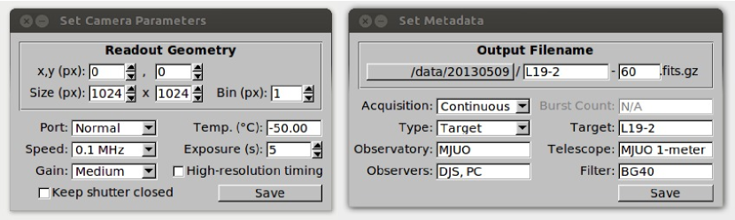
Figure 5: A screen capture showing the acquisition configuration and frame metadata available in the Puoko-nui acquisition software.

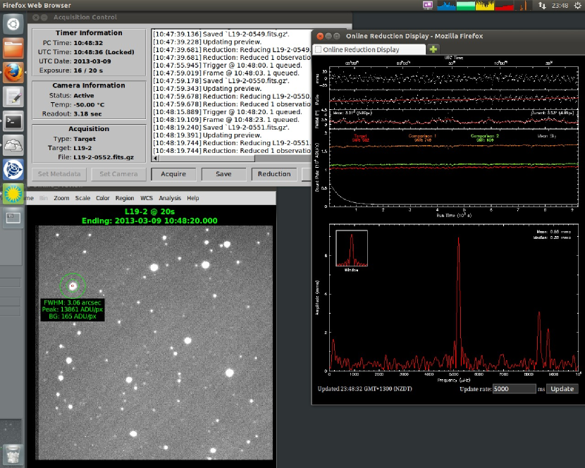
Figure 6: A screen capture showing the online display produced by the acquisition and analysis software during an observation run. The target for these observations is the hydrogen atmosphere pulsating white dwarf L19-2. The star selected in the frame display is a (non-variable) comparison star used to monitor observing conditions.

2.4 Online Reduction

We have developed reduction software, called tsreduce, that performs real-time analysis on the acquired CCD frames, and features offline analysis for generating final data reductions. Synthetic aperture photometry techniques are used to calculate light curves of the target and selected comparison stars. The effects of cloud and atmospheric extinction changes are compensated for by taking the ratio of target and comparison lightcurves, and then any remaining long period trends in the relative lightcurve (resulting from differential colour extinction effects for example) can be minimized by fitting a low order polynomial. This latter procedure is appropriate for studies of the pulsating white dwarf stars, and can be disabled.

The resulting data corresponds to fractional intensity changes in the target star, and are displayed as a plot of milli-modulation intensity (10 mmi = 1% change) versus time. The discrete Fourier transform (DFT) of the data is calculated in amplitude units (which has a more direct physical connection with the data than the more traditional power units) and displayed versus frequency along with the DFT window function.

The reduction display also includes the raw lightcurve plots and an estimate of the mean full-width at half-maximum of the point spread functions of the selected stars. This information enables the observer to monitor atmospheric conditions and telescope focus.

The online reduction has a simple configuration procedure where the user selects the target and comparison stars and surrounding annuli for measuring the background intensity. The aperture size is estimated using a curve of growth technique on the first frame in the exposure sequence. The aperture size is not varied between frames, and so this single-frame estimate is rarely optimal, but is sufficient for the purposes of an online display.

The offline reduction routines allow an optimized final reduction to be calculated by determining the optimum aperture size for each data set, removing the effect of the Earth’s orbital motion from acquisition timestamps (using the excellent sofa library (IAU SOFA Board, 2012)), and combining multiple data sets into a standard output format for analysis. A set of offline analysis routines simplify the identification of frequency modes and estimation of noise limits. The reductions generated by tsreduce compare favorably with other reduction codes such as maestro (Dalessio, 2010), ccd_hsp (Kanaan et al., 2002), and wqed (Thompson & Mullally, 2009).

Fig. 6 shows a screen capture of the acquisition PC mid-way through a typical observing run. The display features three windows showing the online reduction plots, the latest acquired frame, and the instrument control/status window.

2.5 Auto-guiding

The frame preview display provides star positions which can be read by an external program to enable auto-guiding via the science frames. This functionality has been used when operating Puoko-nui North on the 2.1 m Otto Struve Telescope at McDonald Observatory in West Texas.

Puoko-nui South uses a separate dedicated auto-guiding system. The PI camera is mounted on the McLellan 1 m telescope at Mt John University Observatory (MJUO) using the offset guiding mount adapted from the earlier VUW 3-channel photometer (see Sullivan, 2000). This mount contains a 45^∘ mirror with a hole that allows the central field of view to enter the primary camera. The annulus outside the primary field of view is redirected to a secondary camera (an SBIG ST402ME) mounted on a two-dimensional slide mechanism, which allows a nearby star to be independently monitored for auto-guiding purposes. The SBIG camera features a hardware interface that is connected to the telescope control system, and the packaged software (which runs on a separate PC) features a dedicated auto-guiding mode.

The main advantage of this arrangement is that the offset guider configuration has access to a much larger field of view than the primary camera, thus ensuring access to an adequately bright guide star in the often sparse WD fields.

3 Some Results

Observational data obtained using Puoko-nui South that have already appeared in print include observations of the dwarf nova GW Librae (Szkody et al., 2012; Chote & Sullivan, 2013), the helium atmosphere pulsating white dwarf EC 04207$-$4748 (Chote et al., 2013), and the eclipsing double-WD system J0751 (Kilic et al., 2014).

We have undertaken a number of observations using both instruments primarily to ascertain and verify their inherent timing capabilities.

Puoko-nui North in combination with the 2.1 m telescope at McDonald Observatory was used to observe the extremely stable hydrogen atmosphere pulsating white dwarf G117$-$B15A. The impact of evolutionary cooling on this star results in a gradual increase in the 215 s mode period (d$P$/d$t$ $\sim 10^{-15}\,$ s s^-1), which has been detected as a parabolic trend in the observed minus calculated (O$-$C) phase plot over a long observation baseline (see Kepler et al., 2005).

Fig. 7 depicts an excerpt of these observations and, in particular, the bottom panel compares our April 2013 O$-$C phase measurements with the nearly four decades of archival data on this star. This plot provides a simple check of the absolute timing accuracy of the instrument: any systematic time offsets would appear as a vertical offset in the plot. This technique has been used in the past to identify timing issues with the Argos photometer. Our measurements agree with the calculated phase with an uncertainty of $\pm 1.5$ s [Kepler, private communication]. Alternatively, the new observations can be viewed as extending the O$-$C measurements that detect the impact of evolutionary cooling on this star. Referring to Fig. 7, it is interesting to note the general improvement in measurement precision that was obtained by moving from photomultiplier instruments (blue points) to frame transfer CCD measurements (Argos, red points) in 2002. Puoko-nui measurements continue this.

Concurrent observations of the short period eclipsing binary PG 1336$-$018 (Kilkenny et al., 2003) using the two instruments provided a further test of the relative timing integrity of both systems, and are shown in Fig. 8. The individual timings of the primary eclipses are consistent within the photometric uncertainties, which translates to a few seconds.

The high-speed capability of Puoko-nui North was demonstrated by observing the 33 ms optical pulsation of the Crab pulsar in November 2013. A sequence of 5000 5 ms exposures were acquired using the 2.1 m McDonald telescope; these short exposures were achieved using the 10 MHz electron-multiplying readout mode to digitize a $336\times 128$ px region of the CCD with $8\times 8$ binning. The resulting $42\times 16$ px image covered a $30^{\prime\prime}\times 12^{\prime\prime}$ region surrounding the pulsar. In Fig. 9 we present lightcurves of the pulsar and a nearby comparison star folded on a period of 33.689 ms, which was determined from a DFT of the pulsar data. The phase of the main peak was compared with the Jodrell Bank radio ephemeris (Lyne, Pritchard, & Graham-Smith, 1993), and found to agree to within 2.5 $\pm$ 5 ms. This relatively large uncertainty comes from numerical precision limitations in our data reduction pipeline, which is not currently optimized for sub-ms accuracy BJD time conversions.

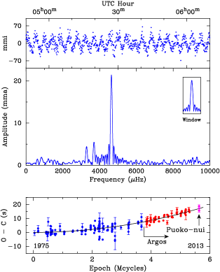
Figure 7: The top two panels depict a short lightcurve segment (in milli-modulation intensity units) and a discrete Fourier transform (in milli-modulation amplitude units) from an observation run on the extremely stable DAV white dwarf pulsator G 117$-$B15A. Data from two runs were acquired in April 2013 using the Puoko-nui North instrument attached to the 2.1 m telescope at McDonald Observatory. The bottom panel compares the measured phases of the dominant 215 s pulsation with the nearly four decades of archival data. Only a representative subset of the measurement uncertainties have been included in the plot to minimise clutter. These new phase measurements are consistent with the theoretical trend (solid line) to within the measurement uncertainties. As well as extending the O$-$C phase data for this pulsator, the measurements also provide a check on the photometer’s absolute timing accuracy (see text and Kepler et al. (2005) for more details).

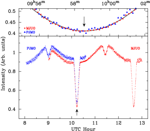
Figure 8: Coordinated and concurrent observations of the near-equatorial short period eclipsing binary PG 1336$-$018 (Kilkenny et al., 2003), obtained in April 2013 using the Puoko-nui North photometer attached to the 0.6 m robotic telescope at Meyer observatory (PJMO), near Clifton, Texas and the Puoko-nui south system with the 1 m telescope at MJUO in NZ. The data in the bottom panel have been offset vertically for clarity. The top panel shows a quartic fit to the eclipse, and demonstrates that the data are consistent to within the photometric uncertainties (given by the point size for the MJUO data, and a factor of two larger for PJMO).

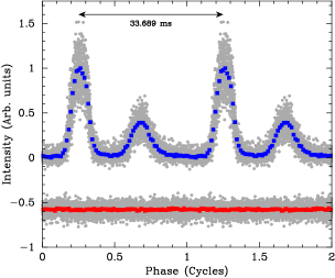
Figure 9: Observations of the Crab pulsar demonstrate the high-speed capabilities of the Puoko-nui North photometer. These data, consisting of a sequence of 5000 5 ms exposures, were obtained using the 2.1 m telescope at McDonald Observatory in November 2013. The plot shows the intensity of the pulsar and a nearby comparison star (grey dots), folded at the primary period of 33.689 ms. This is overlaid with the binned intensity for the pulsar (top, blue) and comparison (bottom, red). The data have been repeated for a second cycle, and the comparison star intensity offset vertically by -0.75 units to improve clarity.

4 Discussion

The two CCD photometers that we describe here have a common GPS timing and instrument control functionality, and they offer a number of distinct advantages for undertaking the demanding task of obtaining precision high-speed time-series photometry.

Both instruments are sufficiently portable that they can be readily transported using airline checked luggage facilities (allowing for the associated weight limitations). The NZ system is regularly transported this way between its Wellington home base and Mt John University Observatory in the South Island. However, transporting the mechanical offset guider box that is an ‘optional extra’ part of Puoko-nui South adds a complicating layer. The Puoko-nui North system is even more portable as the newer PI ProEM camera has all the electronics housed in one unit.

The flexibility of our photometer design makes it relatively simple to integrate with other externally triggered CCD cameras or GPS receivers. In addition, because most of the instrument behavior is defined in software, it would be straightforward to add additional capabilities to e.g. acquire synchronous photometry, read multiple ‘windows’ within the CCD frame, or support a filter wheel in order to carry out automated multi-colour photometry (we have no immediate plans to do this however). Similarly, the online reduction display can be easily modified to show the information most relevant to the target: e.g. the DFT is not useful for many types of time-series photometry, and can be disabled.

Except for the proprietary PI camera interface code, all other software is open source. This includes the C language coding for both the timer firmware and the acquisition and control PC. This software and the hardware schematics for the timer are available on request.

References

- Althaus et al. (2010) Althaus, L. G., Córsico, A. H., Isern, J., & García-Berro, E. 2010, A&ARv, 18, 471
- Chote & Sullivan (2013) Chote, P. & Sullivan, D. J. 2013, in Astronomical Society of the Pacific Conference Series, Vol. 469, 18th European White Dwarf Workshop., ed. J. Krzesínski, G. Stachowski, P. Moskalik, & K. Bajan, 249
- Chote et al. (2013) Chote, P., Sullivan, D. J., Montgomery, M. H., & Provencal, J. L. 2013, MNRAS, 431, 520
- Cocke et al. (1969) Cocke W. J., Disney M. J. & Taylor D. J., 1969, Nature, 221, 525
- Dalessio (2010) Dalessio, J. 2010, BAAS, 42, 215
- Dhillon et al. (2007) Dhillon, V. S. et al. 2007, MNRAS, 378, 825
- Fontaine & Brassard (2008) Fontaine, G. & Brassard, P. 2008, PASP, 120, 1043
- Fontaine et al. (2006) Fontaine, G., Green, E. M., Chayer, P., Brassard, P., Charpinet, S., & Randall, S. K. 2006, Baltic Astronomy, 15, 211
- Hermes et al. (2012) Hermes, J. J. et al. 2012, ApJ, 757, L21
- IAU SOFA Board (2012) IAU SOFA Board. 2012, IAU SOFA Software Collection
- Kanaan et al. (2002) Kanaan, A., Kepler, S. O., and Winget, D. E. 2002, A&A, 389, 896
- Kepler et al. (2005) Kepler, S. O., Costa, J. E. S., Castanheira, B. G., et al. 2005, ApJ, 634, 1311
- Kilic et al. (2014) Kilic, M. et al., 2014, MNRAS, 438, L26
- Kilkenny et al. (2003) Kilkenny, D., et al. 2003, MNRAS, 345, 834
- Kilkenny et al. (2014) Kilkenny, D., Welsh, B. Y., Koen, C., Gulbis, A. A. S., & Kotze, M. M. 2014, MNRAS, 437, 1836
- Kleinman et al. (1996) Kleinman, S. J., Nather, R. E., & Phillips, T. 1996, PASP, 108, 356
- Lyne, Pritchard, & Graham-Smith (1993) Lyne, A. G., Pritchard, R. S., & Graham-Smith, F. 1993, MNRAS, 265, 1003
- Mackay et al. (2001) Mackay C. D., Tubbs R. N., Bell R., Burt D., Moody I., 2001, Proc SPIE, 4306, 289
- Mukadam et al. (2011) Mukadam, A. S., Owen, R., Mannery, E., MacDonald, N., Williams, B., Stauffer, F., & Miller, C. 2011, PASP, 123, 1423
- Nather et al. (1969) Nather, R. E., Warner, B. & Macfarlane, M., 1969, Nature, 221, 527
- Nather & Mukadam (2004) Nather, R. E. & Mukadam, A. S. 2004, ApJ, 605, 846
- Nather et al. (1990) Nather, R. E., Winget, D. E., Clemens, J. C., Hansen, C. J., & Hine, B. P. 1990, ApJ, 361, 309
- Silvotti et al. (2011) Silvotti, R., Fontaine, G., Pavlov, M., Marsh, T. R., Dhillon, V. S., Littlefair, S. P., & Getman, F. 2011, A&A, 525, A64
- Sullivan (2000) Sullivan, D. J. 2000, Baltic Astronomy, 9, 425
- Szkody et al. (2012) Szkody, P., et al. 2012, ApJ, 753, 158
- Thompson & Mullally (2009) Thompson, S. E. and Mullally, F. 2009, J. Phys.: Conf. Ser., 172, 012081
- Winget & Kepler (2008) Winget, D. E. & Kepler, S. O. 2008, Ann.Rev.Astron.Ap., 46, 157