Variable stars in two open clusters within the Kepler 2-Campaign-0 field: M 35 and NGC 2158

Abstract

We present a multi-year survey aimed at collecting (1) high-precision ($\sim$5 milli-mag), (2) fast-cadence ($\sim$3 min), and (3) relatively long duration ($\sim$10 days) multi-band photometric series. The goal of the survey is to discover and characterize efficiently variable objects and exoplanetary transits in four fields containing five nearby open clusters spanning a broad range of ages. More in detail, our project will (1) constitute a preparatory survey for HARPS-N@TNG, which will be used for spectroscopic follow-up of any target of interest that this survey discovers or characterizes, (2) measure rotational periods and estimate the activity level of targets we are already monitoring with HARPS and HARPS-N for exoplanet transit search, and (3) long term characterization of selected targets of interest in open clusters within the planned K2 fields. In this first paper we give an overview of the project, and report on the variability of objects within the first of our selected fields, which contains two open clusters: M 35 and NGC 2158. We detect 519 variable objects, 273 of which are new discoveries, while the periods of most of the previously known variables are considerably improved.

1 Introduction

We present the first report of the multi-year, multi-wavelength photometric survey programme “The Asiago Pathfinder for HARPS-N”, aimed at characterizing variable stars and transiting-exoplanet candidates in five open clusters (OCs). This survey will also select promising targets for accurate HARPS-N@TNG follow-up spectroscopic observations, including exoplanet search programmes.

High precision light curves are required for point-like source periodic variability searches, in particular for planetary transits. Although the chances of catching a transiting planet among the members of a typical sparse OC are rather small (van Saders & Gaudi, 2011), one has to take into account that more than 50 000 stars are detected by our instrument in a typical low Galactic latitude field. This number has to be multiplied by the number of fields monitored during the survey.

Many of the clusters to be studied over the next four years are within the field to be observed by the Kepler-2 Mission (K2 ) campaigns (Howell et al., 2014), following the huge success of the original Kepler mission (Koch et al., 2010). Therefore the timing of our investigation is particularly important, as our observations will be useful extending the baseline of the K2 survey (K2 will observe a given field for only about two months). It will help to identify long-period variables (magnetic cycles, Mira oscillations, etc.) and refine the ephemeris of every transit-like signal which is detectable from the ground.

In this study, we focused on the search for photometric variable sources in one of our selected fields, a patch of sky covering $\sim 0.6$ square degrees and containing both the young, sparse and relatively nearby OC Messier  35 (M 35 = NGC 2168; age 180 Myr; apparent distance modulus $(m-M)_{V}\simeq 10.4$; Kalirai et al. 2003) and the older, more distant, and more concentrated NGC 2158 (1.9 Gyr; $(m-M)_{V}\simeq 14.3$; Bedin et al. 2010).

There are several papers devoted to the search and study of variable stars in these two OCs. For example, Meibom, Mathieu & Stassun (2009) presented a detailed study of the period-colour relation of the rotating stars of M 35, and Mochejska et al. (2004, 2006) studied the variability in a field centred on NGC 2158. In particular they found a candidate transiting-exoplanet (TR1), that we are not able to confirm in this work.

The aim of this investigation is to discover new variable stars in the K2-Campaign-0 field containing the two target OCs, and refine the periods of the already catalogued variables. The paper is structured as follows: in Sect. 2 we report our data-set; in Sect. 3 and 4 the software for the extraction and detrending of light curves is presented; in Sect. 5 we show the tools used for finding variables stars; Sect. 6 is dedicated to the characterization of the variables found in the M 35 and NGC 2158 field; in Sect. 7 we describe the available electronic material. Finally, Sect. 8 summarizes our work.

2 The Database

All data used in this work come from the Asiago 67/92 cm Schmidt Telescope, located at 1370 m on Mt. Ekar (longitude 11${}^{\circ}\!$.5710 E, latitude 45${}^{\circ}\!$.8430 N); this facility belongs to the Astronomical Observatory of Padova (OAPD - Osservatorio Astronomico di Padova), which is part of the Istituto Nazionale di Astrofisica (INAF). The instrument mounted at the Schmidt focus is a SBIG STL-11000M camera, equipped with a 4050$\times$2672 pixel Kodak KAI-11000M detector, having a pixel size of $9\mu\textrm{m}\times 9\mu\textrm{m}$, a pixel scale of 862 mas pixel^-1 (resulting in a 58${}^{\prime}\times$38^′ field of view), electronic gain of 0.92 e^-/ADU, and a readout noise (RON) of 12 e^-/s. The detector is cooled with a thermoelectric Peltier stage, coadiuvated by a radiator with glicole that keeps the operating temperature between $-30$ and $-20$ ^∘C.

Under the long-term observing programme “The Asiago Pathfinder for HARPS-N” (PI: Bedin) four fields were awarded with 80 nights per year, during 3 observing campaigns. Taking into account the weather losses, the number of nights statistically guarantees a minimum of ten nights per year in 3 observational campaigns.

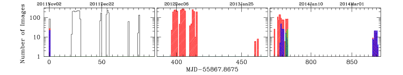
Figure 1: Histogram of the number of images per night collected during the first three campaigns of our programme. The white histogram refers to observations in white light, the red, blue and green histograms refer to observations in the $R$, $B$ and $V$ filters, respectively.

The first observing season was a pilot program. We aimed to have the highest number of stars collected with as many photons as possible. Therefore data were collected in white light (hereafter indicated with filter $N$, for “None”). The unfiltered CCD throughput roughly peaks at $\sim$500 nm. The exposures were long 120 s, long enough to maximize the duty cycle, the cadence, and the dynamic range vs. sky brightness; in this way we were able to measure faint stars (down to $V\sim 20$) and to monitor more stars in this relatively low Galactic-plane field. After analyzing season-one data, we realized that the number of stars was adequate, and that we would be able to follow the same stars in a more thoughtful pass-band, filter $R$, at the cost of slightly increased exposure times (180 s). This would allow better comparison with stellar models and at the same time suppress noise due to larger chromatic and sky-brightness effects. It was also clear from the pilot data-set that adding short exposures of 15 s would have extended the photometric monitoring to a non-negligible sample of saturated stars. There is an additional benefit in alternating short and long exposures besides the increased dynamic range. The use of short exposures means that unsaturated data will still result from the bulk of the stars in the case of extremely good seeing. Short exposures could not be shorter than 15 s because of the reliability on the shutter time. Therefore, when season two and three were accepted we decided to alternate between these short and long exposures in filter $R$ only.

Preliminary results from first two seasons shown that we were able to find many new variables in the field (and 21 variables were found in the photometric series from short exposures, Sect. 5).

Once the variable stars are found, the natural follow up is to collect information about their spectral energy distribution (SED). Therefore, in the third season we collected long exposures alternating both $B$ and $R$ and occasionally we took exposures in $V$. Colour information is particularly important for the characterization of the components of binary systems, not only off-eclipse, but possibly also during the eclipses. Given the successful outcome of this project, additional observing time for follow-up observations in $I$-band has been allocated (unfortunately $U$ is not doable from Asiago) for the M 35 and NGC 2158 field.

During the first year the fine pointing of the field was not optimal. There is an incomplete overlap between the $N$ and $B\,R\,V$ photometric series, resulting in a $\sim$10% sky area not imaged through all the four filters.

Observations included standard calibration data (bias, dark, sky and dome flats) at the beginning and end of each night. In Table 1 we give a log of the observations. Figure 1 shows the histograms of the number of images gathered each night for a given filter during the three seasons.

For the other clusters of this survey we will adopt the following strategy: long + short $R$ exposure in the first season, and multi-filter characterization in the following seasons. With our instrumentation this turns out to be a rather effective strategy, doubling the number of known variables in a relatively well-studied field such as that of M 35 and NGC 2158.

Table 1: Log of observations.

Filter	# Images	Exp. Time	FWHM	median FWHM
		(s)	(arcsec)	(arcsec)
$B$	21	$120$	1.44–5.28	2.65
	258	$180$
	1	$240$
$V$	60	$180$	1.24–2.05	1.43
$R$	1385	$15$	1.35–6.34	2.75
	27	$120$
	2552	$180$
$N$	2692	$120$	1.67–7.05	2.85

3 Data Reduction

For all our reductions we developed custom software tools written in FORTRAN 77 or Fortran 90/95, adapted from the same software described in previous papers by some of the co-authors of this work (we will give in the following brief descriptions and references).

3.1 Pre-reduction

The first stage of our pipeline produces master biases, master darks and master flats for each night. Such master frames are clipped means of the individual calibration images gathered on each observing night. We almost always used dome flats, because they proved to be more accurate and stable than typical sky flats. Flats were bias-subtracted, while science images were dark-subtracted, the master dark being constructed from darks having the same exposure time as the photometric series. The dark-subtracted scientific images were then divided by the bias-subtracted flats of the corresponding filter. The correction was performed by using a custom master-flat field for each night.

3.2 Point Spread Functions

The point-spread function (PSF) of the Asiago Schmidt camera is almost always well sampled, with the exception of a few images collected in the best-seeing conditions. In these cases only the central part of the detector is affected by undersampled PSFs, in which the image quality, measured as the full width at half maximum (FHWM), is below 1.8 arcsec.

To compute the PSF models, we developed the software img2psf_Sch in which our PSF models are derived in a completely empirical fashion. This code follows a similar software developed for WFI@ESO/MPG 2.2m data, and described in depth in Anderson et al. (2006). The Asiago Schmidt’s PSFs are modeled through an array of 201$\times$201 grid points, which super-sample the PSF pixels by a factor of 4 with respect to the image pixels. A bicubic spline is then fitted to interpolate the value of the PSF in between these grid points. Furthermore, in order to model the considerable amount of spatial variations of the PSFs across the field of view of each individual image, we divided the detector in 9$\times$5 regions, and empirically derived the PSFs independently within each of these subregions. A bilinear interpolation is then applied to obtain the best PSF model at any specific location on the detector. This interpolation is performed for every individual star on each frame (Anderson et al., 2006).

3.3 Astrometry

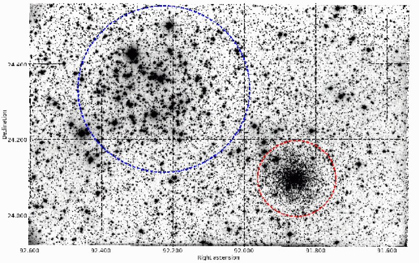
Figure 2: Stacked $R$-filter image from our data. The blue circle marks the M 35 region. The red circle marks the region of NGC 2158.

During the first and the third observing seasons, 25 images with both large and small dithers were collected with the purpose of solving for the geometric distortion of the Schmidt’s camera. We carried out the same self-calibration procedure described in several of our previous works (for example: Libralato et al. 2014; Bellini & Bedin 2010; Bellini, Anderson & Bedin 2011; Anderson et al. 2006). The average geometric distortion is about 1 pixel from corner to the centre of the detector (i.e., $\sim$1 arcsec).

We applied this geometric distortion solution to the raw star positions obtained by fitting our empirical PSFs in each individual image. The distortion-corrected positions of each image were then transformed into a common distortion-corrected reference frame. We employed as reference frame the distortion-corrected positions of the image with the smallest airmass and the best seeing in $R$ (the ID of this image is SC23779).

We considered the most-general linear transformations ( six parameters, i.e., two shifts, rotation, a scale-factor, two skew terms), and derived through a linear least-square fit of the pairs of distortion-corrected coordinates of all (well-measured) stars in common between the two frames (the considered frame, and the reference frame). Such lists of pairs were saved in so-called transformation files.

The consistency of positions on the reference frame tells us how well we are able to transform the coordinate system of one image into another image taken at a different epoch. For the best stars (below saturation, isolated and measured with a high signal to noise ratio) we found a consistency in position of about 20 mas (i.e., $\sim$0.02 pixels). Not enough to determine accurate proper motions for most stars with the available time baseline, but accurate enough to register time series photometry.

3.4 Stacked Images

The transformations from the distortion-corrected coordinates of each image into the reference frame were used to create a stacked, high-S/N image of the field for each filter. The “stack” provides a deeper view of our FOV. The stack for the filter $R$ is shown in Fig. 2. We edited the header of each of these stacked images, adding World Coordinate System keywords, where the absolute astrometric solution was computed matching the 2MASS (Skrutskie et al., 2006) point source catalogue with our sources. The absolute astrometric accuracy of 2MASS is estimated to be about 200 mas.

As part of the material provided in this paper, we make electronically available the astrometrized stacked images for each filter.

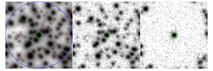
Figure 3: An example of neighbour subtraction. The left panel shows a typical subregion of the stacked image; all detected sources are marked with red circles. The middle panel shows the same for an individual image (SC23893); the target star is located at the centre of the panel (marked by a green circle). The right panel shows the same region after the subtraction of neighbours within a radius of 35 pixels.

3.5 The master star list

Stacked images contain much more information than individual exposures, having essentially a much higher S/N. In the case of the $R$ and $N$ stacks, images have integrated exposure times thousands of times longer than that of a single image. The increased depth means that we could extract more complete and unbiased star lists. Using the same software described in Sect. 3.2, we derived improved star lists from the $R$ and $N$ stacked images, i.e., the deepest ones. Our finding algorithm takes all the local maxima above the local sky with an integrated flux of at least 3 digital numbers (DNs), and isolated by at least 3 pixels from the nearest peak. Positions and fluxes on the stacked images were obtained by simultaneous PSF fitting of the target star and all of its neighbours, in an iterative fashion. The program that performs the finding and simultaneous iterative PSF fit, img2xym_Sch, is an adaptation of the code img2xym_WFI presented in Anderson et al. (2006) and thereby described in details. All the objects in the $R$ star list were then transformed to the astrometric and photometric system of the reference image (ID SC23779). For the $N$ star list, the photometric reference system of image SC25458 was adopted, but coordinates were kept in the $R$ astrometric reference frame.

The above mentioned star lists initially contained a large number of false detections, such as PSF artifacts, warm pixels, etc. We purged the star lists from artifacts and non-stellar objects as follows. Most of the background galaxies were discriminated using the qfit parameter, a diagnostic related to the quality of the PSF fit and described in Anderson et al. (2008). The artifacts of the PSFs are identified using the procedures described in Libralato et al. (2014).

The final $N$+$R$ combined and purged star list contains 66 486 objects and constitutes the catalogue that will be used for the extraction of light curves throughout the following sections. We refer to this catalogue as Master Star List (hereafter, MSL).

3.6 Photometry with and without neighbours

To extract light curves, we developed a parallel code written in Fortran 90/95 which uses OpenMP, in order to run simultaneously on several CPU cores (32 on our workstation). The software takes as input (i) the MSL catalogue as defined in the previous section, (ii) the PSFs described in Sect. 3.2, and (iii) the lists of pairs of coordinates described in Sect. 3.3 (transformation files; stars in common between the MSL and each individual image). In this work we extracted the raw fluxes of all point source detected in the field (i.e., in the MSL) using both PSF and aperture photometry, keeping for the final stage of the analysis only the photometric reduction that minimizes the scatter in the extracted light curves (as we describe in the next sections). We already described the local PSF technique in Sect. 3.2, while aperture photometry is computed through a traditional approach, by running a software pipeline originally developed for the TASTE project (The Asiago Search for Transit time variations of Exoplanets; Nascimbeni et al. 2011). The underlying routines are explained in details in Nascimbeni et al. (2013).

For each target star in the MSL, light curves are extracted in two parallel versions. A first version from the original images, and a second one from images where the neighbours close to the target star were PSF-fitted and subtracted. The neighbour subtraction is done as follows. For each target star we computed 6-parameter local transformations between the MSL reference systems and the distortion-corrected coordinates of stars in the individual image, using the best measured bright, unsaturated and isolated stars located within 500 pixels of the target star. The magnitudes in the two reference systems are also used to register the fluxes in the two photometric systems. With these local transformations, magnitude shifts, and PSFs, the stars of the MSL located less than 35 pixels from the targets are modelled and subtracted from each individual image. Note that such modelling requires an inversion of the geometric distortion solution to obtain the coordinates on the raw image reference system. Figure 3 compares a patch of sky around a typical target star: 1) on the stacked image, 2) in an individual image before the subtraction of the neighbours, and 3) after the neighbour subtraction. After the subtraction procedure, the software performs four parallel reductions: aperture and PSF-fitting photometry of the target star, both on the original frames and on the images where the nearby stars are subtracted. The centroid used for aperture photometry of the target star is computed using the same local 6-parameters transformations described above.

We found that adopting a dynamical aperture, i.e., adapting the radius $r$ of the circular photometric aperture to each image, provides the best photometry. From theoretical computations we know that in the case of a two-dimensional Gaussian PSF the optimum S/N ratio is provided by an aperture radius $r\approx 0.68\times{\rm FWHM}$ (see for example: Mighell 1999). About 72% of the total stellar flux is enclosed within this radius. However, we empirically found that larger apertures result in light curves of smaller scatter for objects at the bright end of our sample. As a compromise, we adopted $r=1\times{\rm FWHM}$, which improves aperture photometry for stars having instrumental magnitudes $<-10.5$, but at the cost of worsening the photometry of faintest stars.

The fitting radius of the PSFs was set to a constant value, equal to 2.65 pixels, as it proved to minimize the scatter of the light curves at all magnitudes.

For all the four reductions we computed the local value of the sky background within a circular annulus of inner radius $r_{\rm in}=7.5\,\sigma$ and outer radius $r_{\rm out}=r_{\rm in}+8$, where $\sigma={\rm FWHM}/2.355$ is the standard deviation of the best-fit Gaussian PSF.

We found that photometry on images after neighbour subtraction performs –on average– better than that computed on original images. This is illustrated in Fig. 4: the top panels display the comparison between the photometric RMS (left panel in the case of aperture photometry, right panel in the case of PSF photometry) obtained from original images (red) and the photometric RMS after neighbour subtraction (blue); the lower panels show the improvement of the neighbour-subtracted algorithm regarding the photometric RMS, averaged over 0.1-mag bins. Therefore, in the following (unless otherwise quoted) we will make use of light curves derived from aperture and PSF photometry obtained from neighbour-subtracted images.

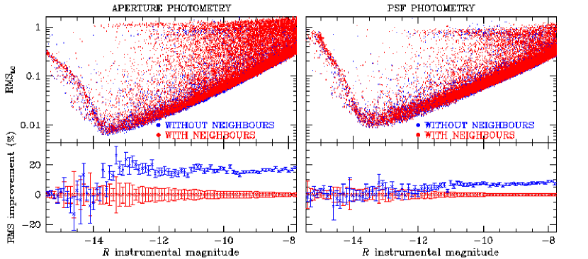
Figure 4: Photometric RMS derived from the original “long” $R$ images (in red) compared to the RMS obtained from the same images after neighbour-subtraction (blue), for both aperture photometry (left) and PSF photometry (right). The lower panels show the percentage improvement of the neighbour-subtracted algorithm on the RMS, averaged over 0.1-mag bins. The error bars are given as the 68.27th percentile of the residuals around the median values.

4 De-trending of Light Curves

To remove residual systematic errors from the light curves derived in the previous section we followed the procedure described in detail by Nascimbeni et al. (2014). For each target star we selected a group of reference stars, which are used to define the local photometric zero point of each target in all the individual images. These reference stars were empirically and iteratively weighted to minimize the scatter on the final differential light curve. A first list of candidate reference stars is selected by computing the median photometric scatter $\sigma$ of the raw light curves as a function of magnitude, then binning over magnitude bins and discarding every source with a RMS $4\sigma$ larger than the median RMS of the corresponding magnitude bin.

A short description of the detrending algorithm follows. Let us consider the $k$-th target star, the $j$-th reference star and the $i$-th epoch where both $k$ and $j$ stars are detected. First we computed the differential light curve $m_{i,k}-m_{i,j}$, its median magnitude and scatter $\sigma_{jk}$, which are then used to compute the initial weights $w_{jk}=1/\sigma^{2}_{jk}$ for each reference star. The final weights are obtained multiplying $w_{jk}$ by two additional factors: $W_{jk}=(1/\sigma^{2}_{jk})\cdot D_{jk}\cdot M_{jk}$. The factor $D_{jk}$ is an analytic function of the relative on-sky position ($\rho_{jk}$) between the reference star and the target star: it is zero within a radius $r_{0}=20$ pix to avoid blending and/or contamination, it is equal to one between $r_{0}$ and $r_{\rm in}=200$ pix, and decreases exponentially with $\rho_{jk}$ from one to zero with a $r_{\rm out}-r_{\rm in}$ scale radius, where $r_{\rm out}=300$ pix. The weight $M_{jk}$ is defined in a similar way, as a function of the magnitude difference $\phi_{jk}=\mid m_{j}-m_{k}\mid$ between the target and the reference star: it is equal to unity when this difference is less than $f_{\rm in}=1.0$ mag, otherwise it decreases exponentially with $\phi_{jk}$ with $f_{\rm out}-f_{\rm in}$ scale radius and $f_{\rm out}=1.75$  mag. The $D_{jk}$ and $M_{jk}$ factors assign a larger weight to reference stars which are closer to the target and of similar brightness, minimizing flux- and position-dependent systematics.

For comparison purposes, we computed two different zero-point corrections. A global zero point correction (GZP) $\tau_{i}$, defined by the formula:

$$m^{\prime}_{i,k}=m_{i,k}-\tau_{i}=m_{i,k}-\langle m_{i,j}-\langle m_{i,j}\rangle_{i}\rangle_{j}$$ (1)

where the notation $\langle x\rangle_{y}$ represents the averaging of $x$ over the index $y$. The output of GZP is then a classical, unweighted differential photometry, where all the reference stars have unitary weight. The local zero point correction (LZP) $\tau^{\prime}$ is computed with an expression equivalent to $\tau$, but this time using the weighted mean of magnitudes of our set of reference stars, where the weights are assigned as $W_{jk}$ and computed as above. Figure 5 compares the scatter of the light curves corrected using the GZP (red) and LZP (blue) detrending algorithms, both for aperture photometry (on the left panels) and for PSF-fitting photometry (on the right panels). The improvement obtained with the LZP correction is evident (10–20%), especially on the bright, non-saturated side of the sample. For this reason, only the LZP light curves are analyzed in the next sections.

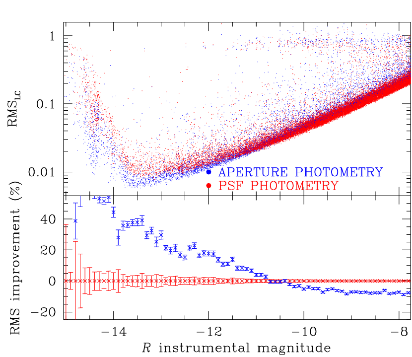
Figure 6: Top panel: photometric rms as function of $R$ instrumental magnitude for PSF photometry (red) and for aperture photometry (blue). Bottom panel: percentage variation with respect to PSF-fitting photometry. This shows that for bright stars (instrumental $R<-10.5$) aperture photometry is better than PSF photometry.

Finally, the RMS of the neighbour-subtracted, LZP-detrended aperture vs. PSF-fitting photometry is compared in Fig. 6, for long exposures in the $R$ filter. It appears that aperture photometry performs on average better than PSF-fitting photometry on bright stars (with instrumental magnitude $<-10.5$), while PSF-fitting photometry gives best results on fainter stars, as expected (see Sect. 3.6). From here on, for each target star in the MSL, only the light curve that provides the smallest overall scatter goes through the next stages of analysis.

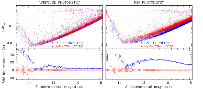
Figure 5: Photometric RMS, obtained from neighbours subtracted images, for GZP-corrected (red) and LZP-corrected light curves (blue). This is shown for both aperture photometry (left) and PSF photometry (right). As in Fig. 4, the bottom panels show the improvement of the LZP algorithm compared to the GZP one.

5 Variable Finding

We employed three different software tools to detect candidate variable stars in our dataset of LZP-corrected, neighbour-subtracted light curves. These are: the Lomb-Scargle (LS) periodogram (Lomb, 1976; Scargle, 1982), the Analysis of Variance (AoV) periodogram (Schwarzenberg-Czerny, 1989) and the Box-fitting Least-Squares (BLS) periodogram (Kovács, Zucker & Mazeh, 2002). All these tools are implemented within the code VARTOOLS v1.202, written by Hartman et al. (2008) and publicly available.

The LS algorithm is most effective in detecting sinusoidal or pseudo-sinusoidal periodic variables. It provides the formal false alarm probability (FAP) as a quantitative diagnostic to select stars with the highest probability to be genuine variables. We searched for more general types of periodic variables through the AoV algorithm, as it is based on variance minimization with phase binning, which is a more flexible approach. As for the LS method, we used the AoV FAP metric $\Theta$ to select stars that have a high probability to be variables. The BLS algorithm is particularly effective when searching for box-like dips in a otherwise flat or nearly flat light curve, such as those caused by detached eclipsing binaries and planetary transits. In order to select good candidates, we used the diagnostic parameter “signal-to-pink noise” (Pont, Zucker & Queloz, 2006), as defined by Hartman et al. (2009). Before running the periodograms, we converted the temporal axis of all light curves from Modified Julian Date (MJD) to the Barycentric Julian Date (BJD) reference frame and Barycentric Dynamical Time (TDB) standard. This standard provides consistency and is much more reliable when comparing observations on very long baselines (Eastman, Siverd & Gaudi, 2010).

We searched for variables independently on both the aperture- and the PSF-fitting light curves (LZP-detrended, from neighbour-subtracted images). These finding algorithms were also run independently on both the $R$ and the $N$ photometric series. On the $R$ light curves we employed LS and AoV to search for variables with periods between 0.01 and 881 days, with a sampling of 0.0005 times the Nyquist one in the frequency space. The period interval set for the BLS algorithm is between 0.5 and 881 days. On the unfiltered light curves ($N$), LS and AOV were set to periods between 0.01–85.5 days (frequency sampling of 0.0005 times the Nyquist one), while BLS between 0.5–85.5 days.

For all three finding methods (LS, AoV, BLS) we applied the procedure illustrated in Fig. 7 to identify the candidate variables. We first constructed the histogram of the detected periods for all the light curves (panel (a) of Fig. 7); spikes in the histogram at this stage are probably associated to spurious periods due to systematic errors, such as instrumental and atmospheric artifacts, which affect a significant fraction of light curves even after the LZP correction. We removed from our catalogue those stars close to the spikes as follows: for each period $P_{0}$ of the histogram of Fig. 7a, we considered a region around it of radius equal to $50\times\delta P$, where $\delta P$ is the bin chosen to build the histogram. We computed the median of the counts of the considered bins, and we flagged $P_{0}$ as spike if the associated counts are 5$\sigma$ above the median, where $\sigma$ is the 68.27th percentile of the sorted residuals from the median value. For the periods associated to spikes, we kept the light curves with low FAP (or high AoV or signal-to-pink-noise), i.e. the light curves above the 99.5th percentile of the $-$FAP (or the AoV or signal-to-pink-noise – see panel (b) of Fig. 7). Panels (c) and (d) show the FAP as a function of the detected period, respectively before and after the spike subtraction. As a last step to select candidate variables, we divided the distribution of panel (d) in 25 period bins and selected only stars above the 97th percentile of $-$FAP.

Finally, we combined the lists of candidates obtained with the three aforementioned methods, and visually inspected each of them. We identified 519 real variables: $BVRN$ light curves are available for 442 of them, while for 37 objects only $BVR$ light curves are available. Nineteen stars have only $N$ light curves, and the remaining 21 have only short exposures in $R$. For the 442 variables in common between $R$ and $N$, we refined their periods with the following recipe. For each star we normalized the $R$ and the $N$ light curves to zero by subtracting the median magnitude. Then we merged the two light curves. In this way we obtained a normalized light curve that spans three years. We ran the VARTOOLS algorithms LS, AoV, and BLS on this normalized light curve using the same parameters described above, to find the best period of the associated variable star. While no modelling can be carried out on such hybrid light curves, the uncertainty on the resulting period is clearly lowered.

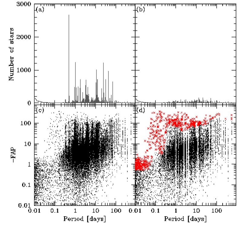
Figure 7: Example of the procedure followed for the extraction of candidate variables from the dataset of light curves in the case of LS algorithm. Panel (a): distribution of the periods obtained from all the light curves; panel (b): distribution of the periods after spikes suppression; panel (c): periods of light curves as a function of FAP for all the stars; panel (d): the same of panel (c) after spikes suppression. The suspected variables are displayed inn red. See text for details.

6 Variables and Light Curves

Amongst the 66 486 stars we found 519 variables, which appear to be point-like sources in the $R$ and $N$ stacked images: 246 of them are already known variable stars and 273 are new ones. The list of all variables is given in Table 2: we provide our identification number, position, period, magnitudes (when available) in $BVRJ_{\rm 2MASS}H_{\rm 2MASS}K_{\rm 2MASS}$, variable type and the cross-identification with known variables.

Figure 8 shows the folded light curves of all the variables listed in Table  2 (all figures are available in the electronic version of the journal): each panel shows, from top to bottom, the light curves in white light $N$ (black), in $R$ (red), $B$ (blue) and $V$ (green) filters. For each filter the y-axis has the same extension in magnitude range. The identification number and the determined period are reported above each panel.

Figure 2 shows the stacked image in the $R$ filter. For illustrative purposes we define two regions around the two clusters: the blue circle which should contain prevalently stars belonging to M 35 inside an arbitrary radius of about $13\aas@@fstack{\prime}8$, while the red circle, with a radius of $6\aas@@fstack{\prime}$0 should include mainly NGC 2158 stars. The $B$ vs. $(B-V)$ color-magnitude diagram (CMD) of the stars within the blue circle is shown in the left panel of Fig. 9. The central panel shows the CMD of the stars within the red circle and in the right panel the CMD of the stars outside both regions. Clearly, the CMD of each region shows contamination by stars from the other two regions.

6.1 Membership

We used the membership probabilities given by Dias et al. (2014) to verify the membership of the identified variable stars. We found 248 common stars between our catalogue and their M 35 catalogue; of these stars, 197 have a probability $\geq 50\%$ to belong to M 35. By matching our catalogue of variable stars with the NGC 2158 catalogue of Dias et al. (2014), we found only 9 stars in common, 5 of which have a membership probability $\geq 50\%$.

The membership probabilities for the two clusters are tabulated in columns 12 and 13 of Table 2.

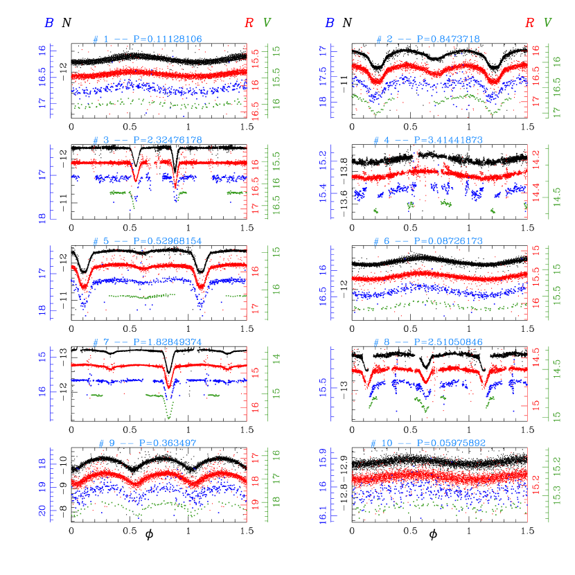
Figure 8: Light curves of the first 10 variables. For each variable star we show (when available) the $N$ (black), $R$ (red), $B$ (blue) and $V$ (green) light curves from top to bottom of each panel.

Table 2: First ten lines of the catalogue of variable stars.

N	$\alpha$(J2000)	$\delta$(J2000)	$P$(days)	$B$	$V$	$R$	$N$	$J_{\rm 2MASS}$	$H_{\rm 2MASS}$	$K_{\rm 2MASS}$	Type	MP${}_{\rm M35}^{7}$	MP${}_{\rm NGC2158}^{7}$	Notes
(1)	(2)	(3)	(4)	(5)	(6)	(7)	(8)	(9)	(10)	(11)	(12)	(13)	(14)	(15-20)
1	91.858422	+24.073243	0.11128106	16.72	15.99	15.78	-11.98	14.316	14.133	13.731	$\delta$Sct	-99.999	62	V373
2	92.561694	+24.006494	0.8473718	17.64	16.72	16.35	-11.32	14.749	14.420	14.230	EB	-99.999	-99.999
3	92.488468	+24.058195	2.32476178	17.06	16.21	15.94	-11.77	14.546	14.286	14.066	EB	-99.999	-99.999
4	91.858693	+24.43994	3.41441873	15.37	14.54	14.28	-13.44	12.974	12.562	12.478	Rot	-99.999	-99.999
5	92.335142	+24.254324	0.52968154	17.20	16.17	15.85	-11.82	14.634	14.014	13.925	EB	96	-99.999	V7 2
6	92.350003	+24.314434	0.08726173	16.40	15.70	15.48	-12.30	14.197	13.888	13.862	$\delta$Sct	0	-99.999	V165
7	92.221929	+24.477042	1.82849374	15.67	15.05	14.79	-12.92	13.491	13.094	12.996	EB	94	-99.999	V155
8	92.058242	+24.510734	2.51050846	15.47	14.81	14.62	-13.14	13.403	13.153	13.062	EB	96	-99.999
9	91.919161	+24.084334	0.363497	19.16	18.17	17.77	-9.86	16.104	15.669	15.293	EB	-99.999	-99.999	V053, 25 4
10	92.106682	+24.257778	0.05975892	16.01	15.33	15.17	-12.63	14.081	13.897	13.718	$\delta$Sct	95	-99.999

Notes.
¹ Kim et al. (2004); ² Hu et al. (2005); ³ Mochejska et al. (2006); ⁴ Meibom, Mathieu & Stassun (2009); ⁵ Jeon & Lee (2010); ⁶ GCVS
⁷ Membership Probabilities for M 35 and NGC 2158 expressed in % : http://www.astro.iag.usp.br/ocdb/ (Dias et al., 2014)

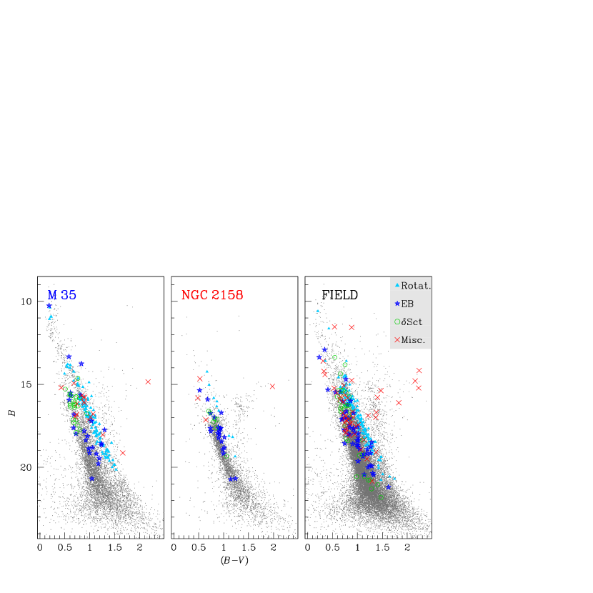
Figure 9: Left panel: stars inside the region delimited by the blue circle (M 35) in Fig. 2. Central panel: stars inside the region delimited by the red circle (NGC 2158) in Fig. 2. Right panel: stars outside the region delimited by the blue and red circles in Fig. 2. Different symbols represent different variable types: azure triangles for rotating stars, blue stars for eclipsing binaries, green open circle for $\delta$ Scuti and red crosses for the other variables.

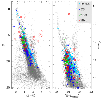
Figure 10: $B$ vs. ($B$$-$$R$) (left panel) and $J_{\rm 2MASS}$ vs. ($N$-$K_{\rm 2MASS}$) (right panel) CMDs. The variable stars are displayed as follows: azure triangles are rotational stars, blue stars are eclipsing binaries, green circles are $\delta$ Sct and red crosses are other variables such as long period, nonperiodic, etc.

Figure 10 shows two CMDs with the largest colour baseline, the CMD in the Johnson filters, $B$ versus $(B-R)$ (left panel), and the CMD obtained combining the white light $N$ (which peaks at $\sim$500 nm) and the 2MASS IR-filters, $J_{\rm 2MASS}$ versus $(N-K_{\rm 2MASS})$ (right panel). In both CMDs we plot the variable stars we have identified, with different symbols and colours according to their type.

6.2 Eclipsing binaries

We extracted 97 light curves of eclipsing binaries (EBs): 41 of these were previously known, the others are new. Many of them are detached systems that, if cluster members, offer the potential for obtaining very precise cluster ages and distances and for testing stellar evolution models, e.g., along the lines of Brogaard et al. (2012). For 9 of these new EBs we have membership probabilities from Dias et al. (2014): we found that 8 of them have a high probability ($\geq 87\%$) to be members of M 35. They are V8, V149, V231, V271, V422, V513, V514 and V517. For NGC 2158 we have no membership information, but looking at Fig. 10 there is a good chance that a substantial fraction of the eclipsing systems in the field of NGC 2158 are members, since they are located along the cluster sequence in the CMD.

The period distribution of the identified EBs is likely to be significantly biased towards short periods and the periods for the longer period systems are uncertain as in common for ground based surveys (Rucinski, Kaluzny & Hilditch 1996). However, complementary observations from K2 should alleviate these issues once analyzed.

6.3 Rotating Stars

We classify 284 of our variables as rotating stars, of which 122 are new discoveries. Their light curves show sinusoidal light variations, mainly due to the starspots that follow the surface rotation. We found that, for many of these stars, the shape of the light curves changes during the three years, but their period remained fairly unchanged (see V18 for an example). Other stars show a sinusoidal shape light curve in one observational run, but their light curve is flat in the other runs (for example V237). There are stars that changed their median magnitude from one year to another, such as V274 or V302.

Figure 11 shows the relation between the period of the variable stars and their $B-V$ (top panel) and $B-K_{\rm 2MASS}$ (bottom panel) colours: the variable stars are in grey, red circles represent the variable stars identified as rotating stars, while blue dots are rotating stars with a probability $\geq 50\%$ to be M 35 members.

Meibom, Mathieu & Stassun (2009) carried out a detailed analysis of the period-$(B-V)$ colour index relation using 310 stars members of M 35, of which 153 are in common with our catalogue.

6.4 $\delta$ Scuti and other variable stars

We identified 67 $\delta$ Scuti stars, 45 of which were previously unknown. In the CMDs, they are mainly located above the main-sequence turn-off of NGC 2158.

Finally, we found 69 variable stars that show long period variations or nonperiodic signals, 21 of these already known. We also found a $\delta$ Cep (V442, already known) and a RRLy (V492).

7 The Electronic Material

The catalogue of all variable stars is available electronically (or upon request to the authors). The catalogue contains the following information: Col. (1) displays is the identification number of the variable in this work; Cols. (2) and (3) are the J2000 equatorial coordinates in decimal degrees; Col. (4) contains the period in days; Cols. (5) to (11) are the calibrated $BVR$, instrumental $N$ and calibrated $J_{\rm 2MASS}H_{\rm 2MASS}K_{\rm 2MASS}$ magnitudes (when magnitudes are not available in a particular filter, they are denoted as 0.0); Col (12) provides the variable type; Col (13) and (14) give the membership probabilities for M 35 and NGC 2158 stars from Dias et al. (2014) (when the membership probability is not available, it is denoted as -99.999); Cols. (15)–(20) give the identification ID in other published catalogues, specifically: Kim et al. 2004, Hu et al. 2005, Mochejska et al. 2006, Meibom, Mathieu & Stassun 2009, Jeon & Lee 2010 and GCVS (in Table 2 we combined cols. (15)–(20) to best fit the table in the manuscript).

For each star in the catalogue we release an astrometrized $43\aas@@fstack{\prime\prime}1\times 43\aas@@fstack{\prime\prime}1$ finding chart for each available filter.

A catalogue of all sources detected in $N$ and $R$ filters is also electronically available. In this catalogue, Cols. (1) and (2) are the J2000 equatorial coordinates in decimal degrees; Cols. (3)–(9) are the calibrated $BVRJ_{\rm 2MASS}H_{\rm 2MASS}K_{\rm 2MASS}$ magnitudes and the instrumental $N$ magnitudes. As mentioned in Sect. 3.4, the astrometrized stacks in $BVRN$ filters are also electronically available.

8 Summary

We present the first results of a long term photometric survey of OC stars conducted with the 67/92 cm Schmidt telescope at Cima Ekar, Asiago. In this paper, we focus on a field which includes the two open clusters M35 and NGC 2158. A total of 6996 58$\times$38 arcmin² images in $B$, $V$, $R$, and white light (no filter) were collected over 2.4 years. We test four different approaches to the stellar photometry: aperture and PSF photometry on the original and neighbour-subtracted images. Aperture photometry on neighbour-subtracted images proves to be the most appropriate method to obtain light curves with the lowest photometric RMS. We also test different approaches to correct our photometry for systematic errors. Our final database includes 66 486 stars. We run different algorithms for the identification of variable stars: i) the Lomb-Scargle periodogram, ii) the Analysis of Variance periodogram, and iii) the Box-finding Least Square periodogram. We identify 519 variables: 97 eclipsing binaries (56 are new identifications), 284 rotational variables (122 new), 67 $\delta$ Scuti variables (45 are new), 69 long period or non periodic variables (50 of them are new), 1 RRLy and 1 $\delta$ Cep. Finally, we cross-correlate our variable star catalogue with previously published catalogues to obtain membership probabilities, and for cross-identification with already know variables. The catalogue with coordinates, $B$, $V$, $R$, 2MASS magnitudes, membership and cross-identification with known variables is made electronically available. The electronic material includes the $B$, $V$, $R$ and white light stacked images. For each variable, a 43.1$\times$43.1 arcsec² finding chart is also made available. M 35 and NGC 2158 are within the field of Campaign-0 of the Kepler 2 Mission. Our survey will therefore complement —and extend in time— the light curves of variable (and not variable) stars covered by K2.

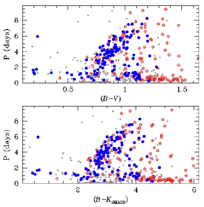
Figure 11: Period vs ($B$$-$$V$) (top panel) and ($B$-$K_{\rm 2MASS}$) (bottom panel) for all the variables (grey dots). Red circles mark the rotating stars, that define the colour-period relation for the stars of M 35. The rotating stars with a membership probability $\geq 50\%$ are displayed in blue.

References

- Anderson et al. (2006) Anderson J., Bedin L. R., Piotto G., Yadav R. S., Bellini A., 2006, A&A, 454, 1029
- Anderson et al. (2008) Anderson J. et al., 2008, AJ, 135, 2114
- Bedin et al. (2010) Bedin L. R., Salaris M., King I. R., Piotto G., Anderson J., Cassisi S., 2010, ApJ, 708, L32
- Bellini, Anderson & Bedin (2011) Bellini A., Anderson J., Bedin L. R., 2011, PASP, 123, 622
- Bellini & Bedin (2010) Bellini A., Bedin L. R., 2010, A&A, 517, A34
- Brogaard et al. (2012) Brogaard K. et al., 2012, A&A, 543, A106
- Dias et al. (2014) Dias W. S., Monteiro H., Caetano T. C., Lépine J. R. D., Assafin M., Oliveira A. F., 2014, A&A, 564, A79
- Eastman, Siverd & Gaudi (2010) Eastman J., Siverd R., Gaudi B. S., 2010, PASP, 122, 935
- Hartman et al. (2008) Hartman J. D., Gaudi B. S., Holman M. J., McLeod B. A., Stanek K. Z., Barranco J. A., Pinsonneault M. H., Kalirai J. S., 2008, ApJ, 675, 1254
- Hartman et al. (2009) Hartman J. D. et al., 2009, ApJ, 695, 336
- Howell et al. (2014) Howell S. B. et al., 2014, PASP, 126, 398
- Hu et al. (2005) Hu J.-H., Ip W.-H., Zhang X.-B., Jiang Z.-J., Ma J., Zhou X., 2005, Chinese J. Astron. Astrophys., 5, 356
- Jeon & Lee (2010) Jeon Y.-B., Lee H.-R., 2010, Publication of Korean Astronomical Society, 25, 167
- Kalirai et al. (2003) Kalirai J. S., Fahlman G. G., Richer H. B., Ventura P., 2003, AJ, 126, 1402
- Kim et al. (2004) Kim H.-J., Park H.-S., Kim S.-L., Jeon Y.-B., Lee H., 2004, Information Bulletin on Variable Stars, 5558, 1
- Koch et al. (2010) Koch D. G. et al., 2010, ApJ, 713, L131
- Kovács, Zucker & Mazeh (2002) Kovács G., Zucker S., Mazeh T., 2002, A&A, 391, 369
- Lang et al. (2010) Lang D., Hogg D. W., Mierle K., Blanton M., Roweis S., 2010, AJ, 139, 1782
- Libralato et al. (2014) Libralato M., Bellini A., Bedin L. R., Piotto G., Platais I., Kissler-Patig M., Milone A. P., 2014, A&A, 563, A80
- Lomb (1976) Lomb N. R., 1976, Ap&SS, 39, 447