THE EMISSION NEBULA Sh 2-174: A RADIO INVESTIGATION OF THE SURROUNDING REGION

Abstract

Sh 2-174 is believed to be either a planetary nebula (PN) or ionized, ambient interstellar medium (ISM). We present in this paper 1420 MHz polarization, 1420 MHz total intensity (Stokes-$I$), and neutral hydrogen (H I) images of the region around Sh 2-174. The radio images address not only the nature of the object, but also the history of the relationship between Sh 2-174 and its surrounding environment. The H I images show that Sh 2-174 sits presently at the center of a $\sim$$1.2\arcdeg$ $\times$ $\sim$$0.4\arcdeg$ cloud (with peak hydrogen density $n_{H}=4\pm 2$ $\rm{cm}^{-3}$). The Stokes-$I$ image shows thermal-emission peaks (with electron densities $n_{e}=11\pm 3$ $\rm{cm}^{-3}$) coincident with the R-band optical nebula, as well as low-surface-brightness emission from an ionized “halo” around Sh 2-174 and from an ionized “plateau” extending southeast from the cloud. The polarization images reveal Faraday-rotation structures along the projected trajectory of Sh 2-174, including a high-contrast structure with “arms” that run precisely along the eastern edge of the H I cloud and a wide central region which merges with the downstream edge of Sh 2-174. The high-contrast structure is consistent with an ionized tail which has both early-epoch (before Sh 2-174 entered the cloud) and present-epoch (after Sh 2-174 entered the cloud) components. Furthermore, our rotation-measure analysis indicates that the ISM magnetic field is deflected at the leading edge of Sh 2-174. The downstream tail and upstream field deflection point to a PN-ISM interaction. Our estimated space velocity for the host white dwarf (GD 561) demonstrates that Sh 2-174 entered the cloud $\sim$27,000 yr ago, and gives a PN-ISM interaction timescale $\lesssim$$2.0\times 10^{5}$ yr. We estimate an ambient magnetic field in the cloud of $11\pm 3$ $\mu\rm{G}$.

1 INTRODUCTION

Sh 2-174 (LBN 598) was first identified as a planetary nebula (PN) by Napiwotzki & Schönberner (1993) on account of its apparent association with the hot white dwarf GD 561 (WD 2342+806). Shortly thereafter, Tweedy & Napiwotzki (1994) confirmed the physical association between Sh 2-174 and GD 561, and, based on the significant westward offset of GD 561 from the center of the nebulosity (see Section 2), termed Sh 2-174 “the planetary nebula abandoned by its central star.” Tweedy & Kwitter (1996) included Sh 2-174 in their atlas of ancient PNe, and noted that the displaced “central” star and sharp western edge of the O III region (see Tweedy & Napiwotzki, 1994) demonstrate two of the principal signs of an advanced interaction between a PN and the interstellar medium (ISM). The general classification of Sh 2-174 as an interacting PN has continued to the present day (see, e.g., Ali et al., 2012, 2013).

Frew & Parker (2010) offer an opposing view of the nature of Sh 2-174, and other low-surface-brightness emission nebulae generally considered to be old PNe (see, also, Kohoutek 1983; Acker & Stenholm 1990; Madsen et al. 2006; Parker et al. 2006; Frew et al. 2010). They believe Sh 2-174 to be a Strömgren zone; i.e., ambient ISM material, ionized and thermally excited by GD 561. This conclusion is based on the absence of an enhanced rim of emission at the leading edge of Sh 2-174, the relatively narrow widths of the Sh 2-174 emission lines, and differences in the kinematics between the ionized gas and GD 561. An additional piece of evidence in favor of a Strömgren-zone interpretation is the evolutionary status of GD 561. Assuming a standard post-asymptotic-giant-branch (post-AGB) evolution, GD 561 is $>$$10^{6}$ yr old (e.g., Blöcker, 1995). This age estimate is a factor $>$4 larger than the estimated ages of even the oldest interacting PNe (see Ali et al., 2012).

Three-dimensional hydrodynamic simulations of the PN-ISM interaction reveal structures that should help distinguish an interacting PN from a Strömgren zone (Wareing, Zijlstra, & O’Brien 2007a). At the early stages of the interaction, a bow shock is formed, even for systems that have relatively low speeds compared to the local ISM (i.e., space velocities, $v_{\rm{S}}\lesssim 25$ km s^-1). The presence of a well-defined bow shock clearly separates interacting PNe from Strömgren zones. However, the bow shock is not stable indefinitely. At the later stages of the PN-ISM interaction, instabilities, which develop over time in the interaction region, begin to disrupt the bow-shock morphology. The disruption happens sooner, and is more severe, for the fastest-moving systems. For some systems, the disturbed PN might have a morphology which resembles ionized, excited ISM. Fortunately, the simulations provide another distinguishing marker. During the interaction, material is ram-pressure stripped at the PN-ISM interface and deposited downstream, forming a tail behind the PN. Though diffuse, tails have been observed behind three interacting PNe: Sh 2-188 (Wareing et al., 2006a), HFG 1 (Xilouris et al., 1996; Boumis et al., 2009), and DeHt 5 (Ransom et al., 2010). In the case of DeHt 5, for which bow-shock disruption is severe (see interaction classification of Ali et al. 2012), the “thick” tail stands as the best evidence of a PN-ISM interaction. In two other cases, namely Sh 2-68 and PHL 932, faint downstream nebulosity could be an ionized trail in the ambient ISM behind an old white dwarf (Frew, 2008; Frew et al., 2010).

Recently, radio polarimetric observations have proven to be a good tool for studying the environments of interacting PNe (Ransom et al., 2008, 2010). Polarimetric observations at frequencies $\leq$3 GHz (wavelengths $\geq$10 cm) are very sensitive to Faraday rotation of the diffuse Galactic synchrotron emission (e.g., Landecker et al., 2010). In propagating through an ionized (and magnetized) medium, the polarized component of the background emission is rotated at wavelength $\lambda$ [m] through an angle

$$\Delta\theta=\rm{RM}\,\lambda^{2}\ [\rm{rad}],$$ (1)

where RM is the rotation measure and depends on the line-of-sight (LOS) component of the magnetic field, $B_{\|}$ $[\mu\rm{G}]$, the thermal electron density, $n_{e}$ $[\rm{cm}^{-3}]$, and the path length, $dl$ $[\rm{pc}]$, as

$$\rm{RM}=0.81\int{B_{\|}\,n_{e}\,dl\ [\rm{rad}\,\rm{m}^{-2}]}.$$ (2)

Even in the relatively low electron-density environment of a PN tail, a rotation at 1420 MHz ($\lambda=21~{}\rm{cm}$) of the background polarization angle of $\Delta\theta\gtrsim 10\arcdeg$ is possible, and leads to a Faraday-rotation structure which is readily observable, provided the background is relatively bright and smooth (Ransom et al., 2010). In the interaction region, where the electron density is higher and the ISM magnetic field likely compressed, the resulting Faraday-rotation structure is even more conspicuous (Ransom et al., 2008). Furthermore, a comparison of the Faraday rotation through the leading and trailing structures may reveal a deflection of the ISM magnetic field around the moving PN (Ransom et al., 2008, 2010). If Sh 2-174 is indeed an interacting PN, evidence in Faraday rotation of an interaction region, tail, and/or deflected field should be “visible” in radio polarimetric images. If, on the other hand, Sh 2-174 is simply a Strömgren-zone, then these identifying features would be absent. Naturally, any ambient structures in the ISM around Sh 2-174, or elsewhere along the LOS, could complicate the picture in either scenario.

In this paper, we present 1420 MHz radio images of the region around Sh 2-174. Our focus is linear polarization, but we also investigate total intensity (Stokes-$I$) and neutral hydrogen (H I) emission. In Section 2, we look at the optical morphology of Sh 2-174, and derive the space velocity of GD 561 relative to the ISM. In Section 3, we describe the preparation of the radio images. In Section 4, we describe the polarization (Faraday rotation), Stokes-$I$, and H I structures which appear in the images. For the Faraday-rotation structures, we quantify changes in the magnitude and/or sign of the RM from one structure to the next. In Section 5, we discuss in detail the structures observed in the radio images, and comment decisively on the nature of Sh 2-174. In Section 6, we give a summary of our results and conclusions.

2 THE OPTICAL MORPHOLOGY OF Sh 2-174 AND THE SPACE VELOCITY OF GD 561

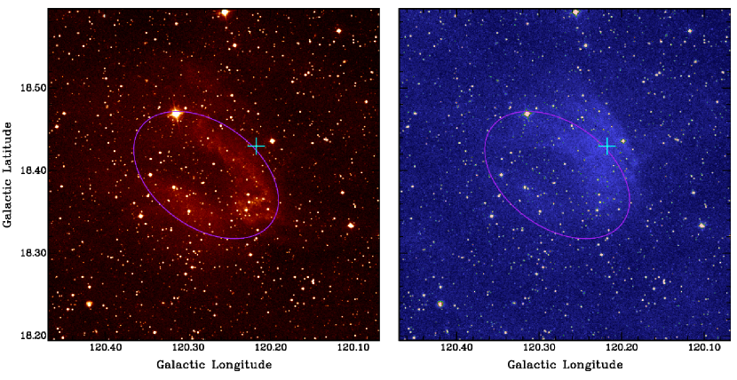
Figure 1: R-band (left) and B-band (right) false-color DSS optical images of a $0.4\arcdeg$ $\times$ $0.4\arcdeg$ region around Sh 2-174. Here and hereafter, images are presented in Galactic coordinates, with Galactic north up and Galactic east to the left. The intensity scale in each image is linear in photon counts, with lighter shades indicating higher counts. The range of intensities in each image has been adjusted to show extended emission in the vicinity of Sh 2-174. The angular resolution is $\sim$1″. The elongated (magenta) ellipse drawn on each image, and on each subsequent image, shows the approximate extent of the R-band “cleft-hoof” structure. The (blue) cross indicates the position of the white dwarf GD 561.

We show in Figure 1 R-band ($\lambda=657$ nm) and B-band ($\lambda=445$ nm) Digitized Sky Survey (DSS) images for a small $0.4\arcdeg$ $\times$ $0.4\arcdeg$ region around Sh 2-174. The R-band emission reveals the so-called “cleft-hoof” morphology seen in $\rm{H}\alpha$ and N II (Tweedy & Napiwotzki, 1994); i.e., an elongated shell-like structure which is brightest in the (Galactic) southwest and fades gradually to the northeast, where it blends with a “halo” of more diffuse emission (see below). We denote the cleft-hoof structure in Figure 1 with an ellipse having angular dimensions $\sim$$12\arcmin$ $\times$ $\sim$$8\arcmin$. Note that GD 561 (indicated by the cross) is located outside the cleft-hoof. The B-band emission, which traces O III (see Tweedy & Napiwotzki, 1994), is approximately centered on GD 561. Its intensity drops fairly steadily east of GD 561, where it meets the cleft-hoof, but drops rather sharply at the west edge. The sharp edge is consistent with a strong shock (Tweedy & Napiwotzki, 1994), as might be expected for a west-moving system (see below) in an interacting PN scanario. On the other hand, if the B-band edge really does signify a shock, then we might expect an enhanced rim along the edge. No such rim is present in either the R-band or B-band. We return to the discussion of the nature of Sh 2-174 in Section 5 after presenting our radio results.

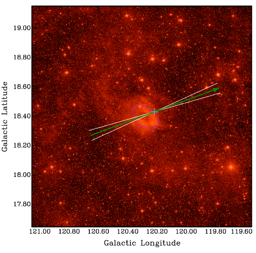
Figure 2: R-band DSS image presented using a logarithmic intensity scale and zoomed out (compared to Fig. 1) to show a $1.5\arcdeg$ $\times$ $1.5\arcdeg$ region around Sh 2-174. The solid (dark green) arrow and adjacent (white) lines drawn on the image indicate the projected space velocity and space-velocity error cone of GD 561. The length of the solid arrow represents the change in the sky position of GD 561 over $\sim$100,000 yrs, with its base starting $\sim$50,000 yr in the past and its tip ending $\sim$50,000 yr in the future. Its present position is again indicated by the cross. The error cone represents largely the error range in the declination component of the proper motion.

To provide a wider-field comparison with our radio images (see Section 4), we show in Figure 2 the R-band DSS image zoomed out to a $1.5\arcdeg$ $\times$ $1.5\arcdeg$ region around Sh 2-174. We use a logarithmic scale here to highlight the diffuse emission. A low-surface-brightness halo surrounds the brighter cleft-hoof structure. Its extent is difficult to estimate, since it fades into very faint “background” structures.

The motion of GD 561 through the ambient ISM frames any discussion of the nature of Sh 2-174, and for this reason we start by deriving the star’s space velocity. The kinematic properties of GD 561 are summarized in Table THE EMISSION NEBULA Sh 2-174: A RADIO INVESTIGATION OF THE SURROUNDING REGION. Since no parallax has been determined for GD 561, its distance, $\rm{d}=415\pm 120$ pc, is estimated via its physical and photometric properties (also given in Table THE EMISSION NEBULA Sh 2-174: A RADIO INVESTIGATION OF THE SURROUNDING REGION). We use the position, distance, proper motion, and radial velocity of GD 561 to estimate the UVW motion through the ISM, where the U component is positive toward the Galactic center, V is positive in the direction of Galactic rotation, and W is positive toward the north Galactic pole (e.g., Johnson & Soderblom, 1987). After correcting for a solar motion of $(\rm{U}_{\sun},\rm{V}_{\sun},\rm{W}_{\sun})=(11.10\pm 1.25,12.24\pm 2.05,7.25\pm 0.62)$ km s^-1 (Schönrich, Binney, & Dehnen, 2010), we find velocity components for GD 561 of $(\rm{U},\rm{V},\rm{W})=(+59.5\pm 7.1,+14.8\pm 3.5,+18.4\pm 3.9)$ km s^-1. The total space velocity of GD 561 through the ambient ISM is then $v_{\rm{S}}=64.1\pm 8.1$ km s^-1, with components on the sky and along the LOS of $63.2\pm 8.2$ km s^-1 and $-10.4\pm 1.2$ km s^-1, respectively. Note, the relatively large fractional uncertainties in the total and sky-projected space velocities reflect largely the uncertainty in the distance estimate. In contrast, the fractional uncertainty in the LOS component of the space velocity reflects largely the uncertainty in $\rm{V}_{\sun}$. The sky-projected space velocity of GD 561, including error cone, is illustrated in Figure 2.

Our estimated $64.1\pm 8.1$ km s^-1 space velocity for GD 561 is very similar to the $66.2\pm 5.8$ km s^-1 value computed recently for this star by Ali et al. (2013). We note, though, that Ali et al. (2013) use older values for the proper motion of GD 561, radial velocity of GD 561, and assumed solar motion. The small difference in the two space-velocity estimates is thus somewhat coincidental. Nevertheless, based on its velocity relative to the ISM, Ali et al. (2013) conclude that GD 561 is a probable thin-disk star. To more confidently establish its membership as either a Galactic thin-disk or thick-disk star, we would need a measurement of GD 561’s parallax.

3 OBSERVATIONS AND IMAGE PREPARATION

The principal observing instrument for the data presented in this paper is the Synthesis Telescope (ST; see Landecker et al., 2000) at the Dominion Radio Astrophysical Observatory (DRAO). To image the region around Sh 2-174, we used seven pointings (or fields) of the ST. We selected the fields so as to have one centered on the position of Sh 2-174, and the remaining six form a hexagonal pattern around the central field. We chose to separate the field centers by $1\arcdeg$. Since the ST antennas have a Gaussian primary-beam response at 1420 MHz with full-width-at-half-maximum (FWHM) of $107.2\arcmin$, the chosen field separation yields a seven-field mosaic with a useful diameter of $\sim$$3.8\arcdeg$.

The ST operates in the radio continuum at 408 MHz and 1420 MHz, and in the 21 cm H I line. The 408 MHz continuum system receives only right-hand circular polarization and is not used in this study. The 1420 MHz continuum system has four 7.5 MHz bands centered on 1407.2, 1414.1, 1427.7, and 1434.6 MHz, respectively, and receives both right-hand (R) and left-hand (L) circular polarizations. The four continuum bands are correlated separately, forming for each band a full set of polarization products (RR, LL, RL, LR), and thus recovering all four Stokes parameters ($I$, $Q$, $U$, $V$). We produced only $I$, $Q$, and $U$ mosaics, and show only those generated by averaging the four bands. The frequency corresponding to the midpoint of the four bands is 1420.4 MHz. The 5.0 MHz band around this frequency is allocated to a 256-channel H I spectrometer. For this study we set the spectrometer to receive a total bandwidth of 1 MHz, providing a radial velocity range of 211 km s^-1 with a channel separation of 0.824 km s^-1 and effective velocity resolution of 1.32 km s^-1. The selected velocity range in the local standard of rest (LSR) frame defined by Schönrich et al. (2010) is $-168\,\mbox{km\,s${}^{-1}$}\geq v_{\rm{LSR}}\leq+43\,\mbox{km\,s${}^{-1}$}$.

The 1420 MHz continuum and H I ST data were calibrated and processed using standard procedures developed at DRAO (e.g., Taylor et al., 2003; Landecker et al., 2010). We note that the wide-field instrumental polarization (i.e., “leakage” from $I$ into $Q$ and $U$) for the seven fields presented in this paper was calibrated using the visibility-plane technique developed by Reid et al. (2008) rather than the older image-plane technique described in Taylor et al. (2003). In producing our seven-field $Q$ and $U$ mosaics, we cut off each individual field at a radial separation $\rho=75\arcmin$ from the field center, since the root-mean-square (rms) residual instrumental polarization error becomes larger than $1\%$ outside this radius. (For point of comparison, we use a more liberal cut-off in producing the $I$ and H I mosaics, namely $\rho=93\arcmin$.) The rms instrumental polarization error is further reduced in the mosaicing process.

The noise level in the central $\sim$$2.5\arcdeg$ of our ST mosaics is approximately uniform due to the arranged overlap between the central field and the outer six fields. In our continuum (band-averaged) $I$, $Q$, and $U$ mosaics, the estimated rms noise level in the central region is $\sim$0.021 K ($\sim$0.16 $\rm{mJy}\,\rm{beam}^{-1}$). Some artifacts are seen above this level in the immediate vicinity of the brightest point sources. In our H I mosaics the estimated noise level (per channel) in the central region is $\sim$2 K rms. Outside the central region the noise level in each mosaic increases due to the corrected primary-beam response in the outer six fields.

The ST is sensitive at 1420 MHz to emission from structures with angular sizes of $\sim$45′ down to the resolution limit of $\sim$1′. To recover structures on the largest spatial scales, we added to our $I$ mosaic single-antenna data from the Stockert-25m (Reich, 1982) and Effelsberg-100m (Reich et al., 2004) surveys and to our $Q$ and $U$ mosaics single-antenna data from the DRAO-26m (Wolleben et al., 2006) and Effelsberg-100m surveys. (We did not add single-antenna data to our H I mosaics.) Striping is present at $\sim$3 times the rms noise level in the low-resolution Stockert-25m and DRAO-26m surveys for the region around Sh 2-174, but filtered out in the first stage of the merging process (i.e., when the data are merged with the Effelsberg-100m data). A full description of the process by which the datasets are combined is given in Taylor et al. (2003). The effective noise levels in the resulting (final) images are unchanged from those noted above for the ST mosaics.

4 RADIO IMAGES OF THE REGION AROUND Sh 2-174

4.1 1420 MHz Polarization

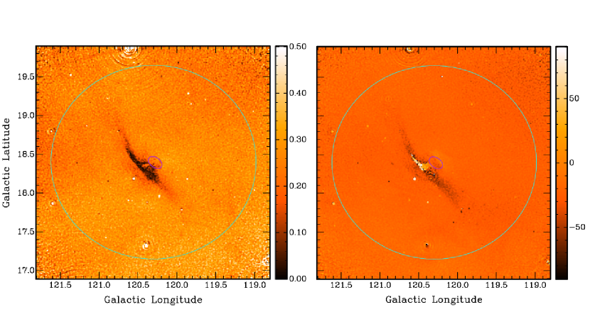
Figure 3: 1420 MHz polarized intensity (left) and polarization angle (right) images of a $3\arcdeg$ $\times$ $3\arcdeg$ region around Sh 2-174. The color choice is arbitrary. The polarized-intensity scale is linear in brightness temperature, with lighter shades indicating higher temperatures. The range of intensities has been cut off at 0.500 K to highlight the diffuse emission. The polarization-angle scale is linear and ranges from $-90\arcdeg$ (black) to $+90\arcdeg$ (white). Note that abrupt black-to-white transitions do not represent large changes in angle, since polarization angles of $-90\arcdeg$ and $+90\arcdeg$ are equivalent (i.e., polarization angles are modulo $180\arcdeg$). The solid $2.5\arcdeg$-diameter (turquoise) circle marks the edge of our central field. The rms noise is approximately uniform inside this circle. The resolving beam at the center of each image is $1.03\arcmin$ $\times$ $0.99\arcmin$ (FWHM), oriented at a position angle (east of north) of $-2\arcdeg$. The resolving beam varies in size over each image by $\sim$2%.

In Figure 3 we show the polarized intensity ($P=\sqrt{Q^{2}+U^{2}-(1.2\sigma)^{2}}$; e.g., Simmons & Stewart 1985, where the last term gives explicitly the noise bias correction) and polarization angle ($\theta_{P}=\frac{1}{2}\arctan{U/Q}$) images at 1420 MHz for the $3\arcdeg$ $\times$ $3\arcdeg$ region around Sh 2-174. Polarization angles are measured east of north. The small $\sim$$12\arcmin$ $\times$ $\sim$$8\arcmin$ ellipse denotes (as in Figures 1 and 2) the approximate extent of the R-band nebula. The large $2.5\arcdeg$-diameter circle outlines the central field, within which the rms noise is approximately constant (see Section 3). The images reveal a thin structure next to Sh 2-174 which stands out, due to Faraday rotation, in stark contrast to the relatively smooth surroundings: the polarized intensity is significantly lower than that of the surroundings, and the polarization angles show large variations and have a mean value significantly different from that of the surroundings. (We describe the mechanism and effects of the Faraday rotation in detail below.) The structure is aligned approximately northeast-southwest, with its northern tip bending slightly north-northeast and its southern tip bending slightly south-southwest. At its midpoint, this $S$-shaped structure (for lack of a better descriptor) stretches westward into a “bridge” which appears to terminate at the eastern edge of Sh 2-174. The images also reveal lower-contrast Faraday-rotation features which extend east and west of the midpoint of the $S$-shaped structure.

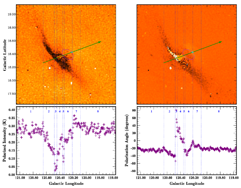
Figure 4: Top panels: The polarized intensity (left) and polarization angle (right) images from Fig. 3 zoomed in to show the same $1.5\arcdeg$ $\times$ $1.5\arcdeg$ region presented in Fig. 2. The projected space velocity and current position of GD 561 are indicated (see Fig. 2 caption). Bottom panels: Polarized intensities (left) and polarization angles (right) along the projected trajectory of GD 561. The (blue) dotted lines show the east-west extent of the eight slice-regions described in the text.

To see more detail in the Faraday-rotation structures around Sh 2-174, we show in Figure 4 (top panels) the central $1.5\arcdeg\times 1.5\arcdeg$ region of our polarized intensity and polarization angle images. We include (as in Figure 2) a vector indicating the projected space velocity of GD 561, as well as a marker for the current position of GD 561. Not coincidentally (see Section 5), some of the more distinct boundaries and systematic variations in the Faraday-rotation structures can be traced along the projected space velocity vector. To accentuate this fact, we present in Figure 4 (bottom panels) polarized intensity and polarization angle slices along this line. We have identified eight slice-regions whose edges represent a clear boundary or a change in the pattern of the variations. To summarize, briefly, regions 1 and 8 are the “surroundings.” Region 2 is the first indication in the images (moving from east-to-west) of a change from the surroundings. Region 3 marks the narrow eastern boundary with the $S$-shaped structure. Region 4 corresponds to the bridge that connects the $S$-shaped structure to Sh 2-174. Region 5 marks the narrow eastern (or downstream) boundary of Sh 2-174. Region 6 runs across Sh 2-174, from the downstream boundary to approximately the position of GD 561. Finally, region 7 runs across the relatively wide western (or upstream) boundary of Sh 2-174. In Section 4.1.1, we describe the actions of Faraday rotation in each of our slice-regions. In Section 4.1.2, we look at the Faraday-rotation behavior along the major axis of the $S$-shaped structure. In Section 4.1.3, we describe the analysis which yields estimates of the RMs through the various structures.

4.1.1 Faraday rotation in structures along the projected trajectory of GD 561

We describe here the Faraday rotation in the eight identified slice-regions along the projected space velocity vector of GD 561 (see Figure 4). We begin with the surroundings (regions 1 and 8), which set comparables for the observed polarized intensities and polarization angles, and then proceed westward through regions 2–7. Some mention is made here of the physical conditions responsible for the Faraday rotation, but we save a more complete discussion for Section 5.

Regions 1 and 8: The polarized intensities and polarization angles in these slice-regions are approximately constant within the noise. Moreover, the mean values for region 1 are very similar to those for region 8: $0.271\pm 0.026$ K and $-24\arcdeg\pm 3\arcdeg$ in region 1, and $0.275\pm 0.023$ K and $-22\arcdeg\pm 2\arcdeg$ in region 8. These slice values do not differ (within the quoted standard deviations) from mean values taken over larger, two-dimensional, versions of regions 1 and 8 having the same longitude boundaries. In other words, the slices are fair representations of the greater surroundings.

Region 2: Moving east-to-west across this region, we see the polarized intensity decrease from the mean region 1 value, and the polarization angle rotate systematically clockwise (i.e., to more negative values) compared to the mean region 1 value. To assist the reader in interpreting these variations, we give here a description of the mechanism through which Faraday rotation affects the observed intensities and angles. The specifics apply to region 2, but the principles apply to each of regions 2–7. The mechanism is as follows: diffuse linearly-polarized background passes through region 2, which is ionized and magnetized, with one or more of the electron density, magnitude of the LOS magnetic field, and path length increasing east-to-west. Equivalently, we can say there is a RM gradient across region 2. The background is thus Faraday rotated (see Equation 1), with the degree of Faraday rotation increasing with more westward sightlines. The rotated background is then (vector) added to the foreground to produce the observed values for the polarized intensity and polarization angle. Not surprisingly, the polarization angles for region 2 differ from those of region 1, since region 1 results from the addition of the unrotated background and the foreground. Also, the polarized intensities for region 2 are lower than those in region 1, since the rotated background is not as well aligned with the foreground as is the unrotated background. This effect is referred to as localized depth depolarization or background-foreground cancellation (e.g., Gray et al., 1999; Uyanıker et al., 2003). Beam depolarization, due to systematic variations or stochastic fluctuations in the polarization angle on scales smaller than the beam size ($\sim$$1\arcmin$ for the ST), can also reduce intensities (e.g., Gray et al. 1999; Uyanıker et al. 2003; Haverkorn, Katgert, & de Bruyn 2004). Via the technique described in Section 4.1.3, we estimate a mean RM in region 2 of $-6\pm 2$ $\rm{rad}\,\rm{m}^{-2}$, and find that beam depolarization accounts for $\sim$$30\%$ of the intensity reduction. (Note, the relative contribution of beam depolarization is higher in the low-intensity “knots” seen outside the slice but within the same longitude boundaries.) Since the systematic variation in polarization angle observed in region 2 amounts to only $\sim$$1.5\arcdeg$ over a beamwidth, the estimated $\sim$$30\%$ beam depolarization must arise from stochastic fluctuations. The most likely cause of such fluctuations is turbulence.

Region 3: This narrow region is marked by near-zero polarized intensities and rapid variations in the polarization angles. Moving east-to-west, the polarization angles first appear to jump pseudo-randomly from negative to positive values, and then settle into a rapid clockwise rotation. It may be, however, that the rotation is systematically clockwise throughout region 3, with the rotation being extremely rapid over the first three data points. This interpretation is believable to the eye, especially if we ignore the second point. Indeed, the $\sim$$+11\arcdeg$ value for this point can easily be explained as an east-to-west average, over a beamwidth, of values near $-90\arcdeg$ and values near $+90\arcdeg$. Moreover, a systematic clockwise rotation across region 3 is consistent with the change in mean RM between regions 2 and 4. In any case, the result of the rapid polarization-angle variations is strong beam depolarization across region 3. We do not estimate a mean RM for this region.

Region 4: Moving east-to-west across this region, we see a general increase in polarized intensity and a systematic clockwise rotation of polarization angle. These trends demonstrate that the rotated background aligns better with the foreground for western sightlines than for eastern sightlines. We estimate a mean RM in this region of $-44\pm 5$ $\rm{rad}\,\rm{m}^{-2}$. This is the largest absolute RM value found for any of the observed Faraday-rotation structures, indicating that region 4 has the highest combination of electron density and LOS magnetic field anywhere within $\sim$$1.5\arcdeg$ of Sh 2-174.

Region 5: This narrow region is marked by a sharp drop in polarized intensity and an apparent discontinuity in polarization angle. The discontinuity is supported, and indeed magnified, by a comparison of the mean RMs found for regions 4 and 6. What looks like a $\sim$$-20\arcdeg$ (east-to-west) change in polarization angle between the second and third data points, is more likely a $\sim$$+160\arcdeg$ change. For the intensities, however, it is the effective polarization-angle change, modulo $180\arcdeg$, that contributes to background-foreground cancellation and beam depolarization. So, while the drop in intensity across region 5 is significant, it is not as severe as that seen in region 3. We do not estimate a mean RM for this region.

Region 6: Moving east-to-west across this region, we see, after the first five points, a systematic counter-clockwise rotation in polarization angle. The polarized intensity is approximately constant for the first five points, increases to a peak value just west of the midpoint, and finally drops to a local minimum at the transition with region 7. Not surprisingly, the intensity peak is coincident with polarization angles which have approximately the same value as the mean surroundings; i.e., background-foreground cancellation is a minimum at this location. The drop in intensity at the transition between regions 6 and 7 is due to a combination of background-foreground cancellation and beam depolarization. The systematic east-to-west change in polarization angle from values more negative than those for the mean surroundings to values more positive than those for the mean surroundings indicates a change in the sign of the RM over region 6. Physically, this change demonstrates a reversal in the direction of the LOS component of the magnetic field moving east-to-west across region 6. We estimate a mean RM in this region of approximately zero ($\rm{RM}=-1\pm 2$ $\rm{rad}\,\rm{m}^{-2}$).

Region 7: Moving east-to-west across this region, we see the polarization angle rotate clockwise, level off, and then continue rotating clockwise to the transition with region 8. Interestingly, the eastern half of region 7 has a mean polarized intensity which is slightly higher than that of the surroundings. There are two possible explanations for this: First, there could be an enhancement of the diffuse polarized emission somewhere along these sightlines. This is very unlikely, given that these enhanced intensities span an angle of just $\sim$$0.1\arcdeg$. Second, instead of background-foreground cancellation, we could have for these sightlines background-foreground enhancement. This is possible if the background was rotated in the eastern half of region 7 so as to align better with the foreground than it does in the surroundings. This interpretation is consistent with the average background and foreground properties we estimate in Section 4.1.3. We estimate a mean RM in this region of $+8\pm 2$ $\rm{rad}\,\rm{m}^{-2}$.

4.1.2 Faraday rotation along the $S$-shaped structure

The $S$-shaped structure is the largest contiguous Faraday-rotation feature in the observed region around Sh 2-174. It runs $\sim$1.2$\arcdeg$ from top to bottom, and varies slightly in width from $\sim$0.1$\arcdeg$ for the north “arm” to $\sim$0.15$\arcdeg$ for the bridge and south “arm”. Internally, the $S$-shaped structure contains several notable substructures. Along with the bridge, the most eye-catching is the jagged-edged, $\sim$0.3$\arcdeg$-long “finger” seen most easily in polarization angle. We encountered the finger in Section 4.1.1 as region 3, the eastern boundary of the central bridge. In two dimensions, we see that the finger extends from the bridge into the north arm. The jagged outline of the finger is $\sim$1$\arcmin$ wide and characterized by near-zero polarized intensities and variations in polarization angle of $>$70$\arcdeg$ (see slice data for region 3).

Unlike the north arm’s finger, the south arm has no discernible extended substructures. Immediately southwest of the bridge, we see 1$\arcmin$–2$\arcmin$-wide fluctuations in both polarized intensity and polarization angle. Moving farther away from the bridge on the south arm, we continue to see small-scale fluctuations, but with maximum deviations decreasing with angular separation from the bridge. A similar trend is seen in the small-scale fluctuations beyond the finger in the north arm. Averaging over 3–4 fluctuations a separation $\sim$$0.3\arcdeg$ from the center of the bridge, we estimate for each arm $\rm{RM}=-16\pm 5$ $\rm{rad}\,\rm{m}^{-2}$. Over the same area, we also estimate that beam depolarization accounts for $\sim$$50\%$ of the intensity reduction. The visible fluctuations and high degree of beam depolarization point to considerable turbulence in the arms of the $S$-shaped structure.

4.1.3 RM analysis

In the absence of a foreground, and assuming the background is uniform across the observed region, the RM in a localized structure can be estimated directly by taking the difference in polarization angle between sightlines on the structure and sightlines on the surroundings. When the foreground cannot be ignored, as for the Faraday-rotation structures around Sh 2-174, the scenario is more complex. Nevertheless, it is possible, through trial and error, to construct a model that resolves the differences in observed polarized intensity and polarization angle between the surroundings and each structure of interest (e.g., Wolleben & Reich, 2004; Sun et al., 2007). The model parameters include for each structure the background intensity and angle, the foreground intensity and angle, the RM in the structure, and the degree of beam depolarization on the structure. As in the simple case for a negligible foreground, the model assumes that the background (and now also the foreground), are the same for sightlines on the surroundings and each structure of interest. We believe this to be a fair assumption for the $1.5\arcdeg\times 1.5\arcdeg$ region around Sh 2-174, since, outside the Faraday-rotation structures themselves, the observed intensities and angles are approximately constant. Using this trial-and-error technique, we were able to find an acceptable range of background and foreground values, and estimate the RM and degree of beam depolarization for each of regions 2, 4, 6, and 7 along the projected trajectory of GD 561, as well as for the arms of the $S$-shaped structure. We did not construct models for regions 3 and 5, since these regions show rapid variations in intensity and angle over a small number of pixels. Our model background has polarized intensity $0.14\pm 0.02$ K and polarization angle $-30\arcdeg\pm 10\arcdeg$, while our model foreground has polarized intensity $0.13\pm 0.02$ K and polarization angle $-15\arcdeg\pm 10\arcdeg$ (see also Table 2). Our estimated mean RMs are given in the appropriate sections above and presented in Table 2. Our estimated beam depolarization values are also presented in Table 2. We note that, while we present only the mean RMs, the relatively smooth variations in polarization angle across each modeled region demonstrate that the RMs also vary smoothly across each region. We note, also, that the quoted RM uncertainties are dominated by the rms variations in the observed polarization angles, and not by the uncertainties in the model background and foreground. In fact, because the background and foreground must add to produce the surroundings, the estimated RMs are relatively insensitive to even larger (forced) changes to either the background or foreground. Nonetheless, it is reassuring that Galactic three-dimensional emission models (Sun et al., 2008; Sun & Reich, 2009) also produce for this part of the sky a background ($d\gtrsim 415$ pc) and foreground ($d\lesssim 415$ pc) with polarized-intensity ratio $\sim$1 and polarization-angle difference $\sim$10–15$\arcdeg$.

RMs estimated via modeling are subject to ambiguity. For most sightlines around Sh 2-174, we adopt the smallest possible rotation, since the observed polarization angles vary by $\lesssim$$20\arcdeg$ as we move from the surroundings to the structure of interest. The exception is region 4. The smallest mean RM through region 4 is $\rm{RM}=+26\pm 5$ $\rm{rad}\,\rm{m}^{-2}$. This option is inconsistent with the transition in polarization angle from $-90\arcdeg$ (black) to $+90\arcdeg$ (white) at the region’s east, north, and south boundaries (see Figure 4). The next smallest mean RM for region 4 is $\rm{RM}=-44\pm 5$ $\rm{rad}\,\rm{m}^{-2}$. A negative RM more naturally explains the observed transitions.

Since the ST has four bands, we looked for point sources that could be used to probe the RMs on sightlines through regions 2–7 and the arms of the $S$-shaped structure (e.g., Savage, Spangler, & Fischer, 2013). Unfortunately, no point sources are so fortuitously located. However, it is also possible to estimate RMs directly from the diffuse emission, provided the polarization angles in each band have relatively small rms scatter. We performed a four-band analysis (see Brown, Taylor, & Jackel 2003; Geisbuesch et al. 2014 in prep.) on the diffuse emission at the midpoints of each of regions 2, 4, 6, and 7, and found RM values consistent with the mean values estimated using the modeling method: a region-by-region comparison shows that the sense of rotation determined by each method is the same and that the magnitude determined by each method differs by no more than the combined errors. The four-band result for region 4 ($\rm{RM}=-39\pm 7$ $\rm{rad}\,\rm{m}^{-2}$) validates the argument given above in favor of a negative RM for region 4.

4.2 1420 MHz Total Intensity

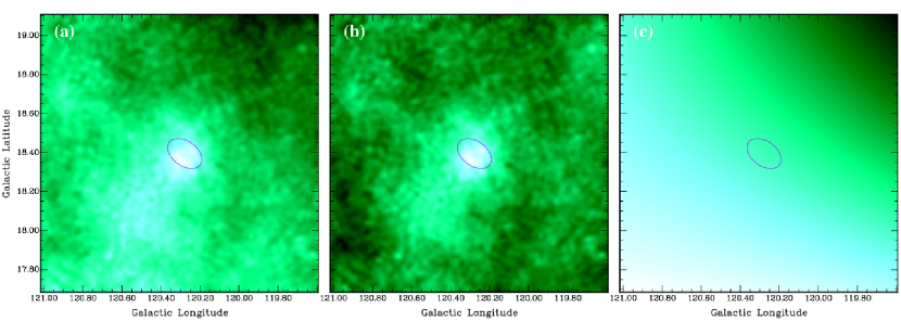
Figure 5: 1420 MHz total intensity ($I$) image of a $1.4\arcdeg$ $\times$ $1.4\arcdeg$ region around Sh 2-174 (panel (a)). Point sources are removed and the image smoothed to $2\arcmin$. Panel (b) is the $I$ image presented in panel (a) after subtraction of a twisted plane (panel (c)). The color choice is arbitrary. The intensity scale in each panel is linear in brightness temperature, with lighter shades indicating higher temperatures. The intensities range before subtraction from 4.264 K to 4.515 K (panel (a)) and after subtraction from $-0.065$ K to 0.142 K (panel (b)). The intensities in the twisted plane vary smoothly from 4.284 K to 4.424 K (panel (c)).

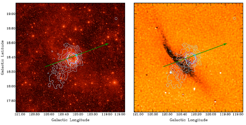
Figure 6: DSS R-band (left) and polarized intensity (right) images from Figs. 2 and 4, respectively, with 1420 MHz $I$ contours overlaid (in light blue). The contours were generated from the image presented in Fig. 5b. Contour levels increase by 0.014 K (the estimated rms “off-source” variations) starting at a brightness temperature of 0.042 K. The 0.098 K contour is drawn thicker than the remaining contours. The projected space velocity and current position of GD 561 are indicated (see Fig. 2 caption).

In Figure 5a we show the total intensity ($I$) image for the region around Sh 2-174, after removing point sources and smoothing the resulting image (modestly) to $2\arcmin$. In Figure 5b we show the $I$ image after also subtracting a twisted plane representative of the diffuse “background” (Figure 5c). The mean residual brightness temperature (in Figure 5b) away from the emission surrounding Sh 2-174 is $<$0.01 K, with rms variations 0.014 K. In Figure 6 we superimpose $I$ contours (generated from the image presented in Figure 5b) on the DSS R-band and 1420 MHz polarized intensity images for the region around Sh 2-174. The brightest $I$ emission (i.e., that within the thick 0.098 K contour) is coincident spatially with Sh 2-174. Moreover, the localized $\sim$0.14 K and $\sim$0.13 K peaks align precisely (i.e., within $\sim$$1\arcmin$) with the mid-lines of the southeast and northwest “rims” of the R-band cleft-hoof structure. The $I$ emission on and near these peaks almost certainly shares the same (thermal) origin as the R-band emission. (No enhancement is seen in the 408 MHz emission at or near the position of Sh 2-174, which further supports a thermal origin for the 1420 MHz $I$ emission.) In contrast, the brightest $I$ emission has no overall counterpart in Faraday rotation. This is perhaps not surprising, since thermal emission requires only relatively high electron densities, while Faraday rotation also requires a relatively strong LOS magnetic field.

At brightnesses just below $\sim$0.10 K, the $I$ emission forms a $\sim$$0.4\arcdeg$-diameter halo around Sh 2-174. A halo is also present in the R-band emission. Curiously, at even lower brightnesses ($\sim$0.04 to $\sim$0.06 K), the $I$ emission stretches southeast into an extended “plateau” $\sim$$0.4\arcdeg$ long and $\sim$$0.3\arcdeg$ wide. No similarly elongated structure is seen in either R-band emission (above the DSS “background”) or Faraday rotation. However, the plateau does pass directly across the bridge of the $S$-shaped structure.

4.3 Neutral Hydrogen (H I)

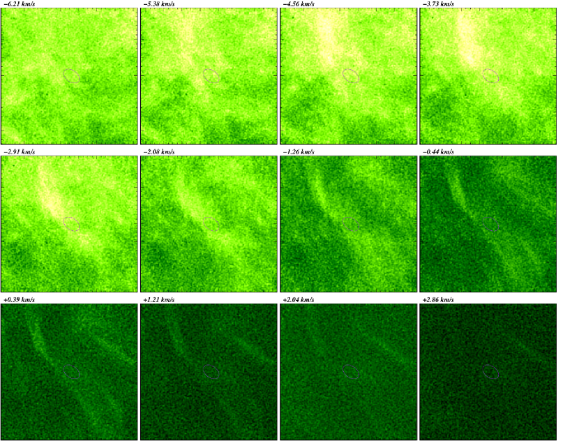
Figure 7: Continuum-subtracted H I images of a $1.5\arcdeg$ $\times$ $1.5\arcdeg$ region around Sh 2-174 region. (The displayed region is the same as that presented in Fig. 2 and Fig. 4.) The twelve displayed velocity channels are a subset of the 256 total channels. The velocity with respect to the Schönrich et al. (2010) LSR is indicated for each image. The color choice is arbitrary. The intensity scale is linear in brightness temperature, with lighter shades indicating higher brightness temperatures.

In Figure 7 we show H I images of the region around Sh 2-174 for twelve consecutive velocity channels between $v_{\rm{LSR}}=-6.21$ km s^-1 and $v_{\rm{LSR}}=+2.86$ km s^-1. The central 8–10 channels in this range contain emission from two local (i.e., $v_{\rm{LSR}}\sim 0$ km s^-1) H I clouds – one which runs approximately northeast-to-southwest through the center of the displayed region, and one which is confined more to the northwest corner of the region. The full spatial extent of these clouds is best seen in channels which are otherwise essentially empty (i.e., $v_{\rm{LSR}}=-0.43\,\mbox{km\,s${}^{-1}$}$, $+0.39\,\mbox{km\,s${}^{-1}$}$, $+1.22\,\mbox{km\,s${}^{-1}$}$). The cloud in the northwest corner is of no particular interest here. The more elongated, central cloud, however, has the same position, orientation, and profile as the $S$-shaped, Faraday-rotation structure.

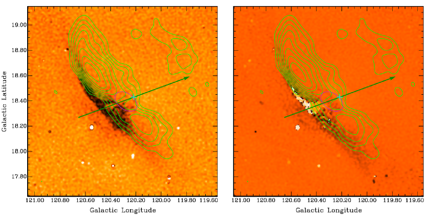
Figure 8: Polarized intensity (left) and polarization angle (right) images from Fig. 4 with H I contours overlaid (in green). The contours were generated after averaging the eight central velocity channels ($v_{\rm{LSR}}=-4.56$ km s^-1 to $v_{\rm{LSR}}=+1.21$ km s^-1) presented in Fig. 7, subtracting a twisted plane, and smoothing the resulting H I image to $5\arcmin$. Contour levels increase by 0.7 K (the estimated rms “off-source” variations) starting at a brightness temperature of 2.1 K. The projected space velocity and current position of GD 561 are indicated (see Fig. 2 caption).

To showcase the correspondence between the elongated H I cloud and the Faraday-rotation structures, we superimpose in Figure 8 H I contours on the 1420 MHz polarized intensity and polarization angle images. The H I contours were generated after averaging the eight central channels ($v_{\rm{LSR}}=-4.56$ km s^-1 to $v_{\rm{LSR}}=+1.21$ km s^-1), subtracting a twisted plane representative of the “background,” and smoothing the resulting image to $5\arcmin$. The mean residual brightness temperature away from the cloud (after subtraction of the twisted plane) is $<$0.5 K, with rms variations 0.7 K. The superposition demonstrates clearly that the Sh 2-174-centered position of the H I cloud is not a LOS coincidence. The neutral material in this cloud and the ionized material in the Faraday-rotation structures (and Sh 2-174) are physically interconnected: The arms of the $S$-shaped structure run precisely along the sharp eastern edge of the cloud. Moreover, the finger (seen best in the polarization angle image), which stretches north from the midpoint of the $S$-shaped structure, actually fills a slight indentation in the eastern edge of the cloud. Moving west from this boundary, along the projected trajectory of GD 561, we see the ionized material (in the Faraday-rotation bridge) “puncture” the neutral material. Sh 2-174 itself sits in a low-surface-brightness cavity at approximately the midpoint of the cloud.

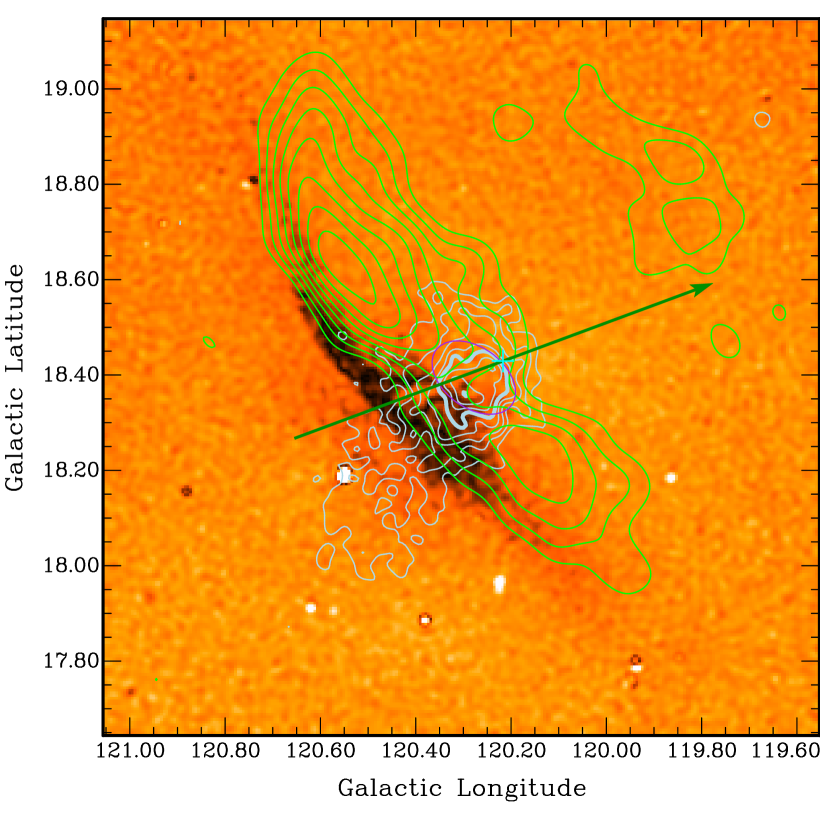
Figure 9: Polarized intensity image from Fig. 4 with both $I$ (Fig. 6) and H I (Fig. 8) contours overlaid. The projected space velocity and current position of GD 561 are indicated (see Fig. 2 caption).

In Figure 9 we superimpose both the H I and $I$ contours on the 1420 MHz polarized intensity image, yielding an all-in-one radio image. We noted in Section 4.2 that there is no overall correspondence between the $I$ emission and the Faraday-rotation structures seen in polarization, but that the extended $I$-emission plateau passes across the bridge of the $S$-shaped structure. We see now, in comparing the contours, that the low-surface-brightness $I$ emission is shaped by the H I cloud: the $I$ halo is indented northeast and southwest of Sh 2-174 at precisely the locations where the H I emission is brightest, while the $I$ plateau extends southeast through the depression (including Sh 2-174-filled cavity) between the H I-emission peaks. We discuss the likely origins for the halo and plateau in Section 5.4 and Section 5.7, respectively.

5 DISCUSSION

5.1 Electron Density in Sh 2-174

We can derive the emission measure (EM) for Sh 2-174 from the thermal $I$ emission coincident with the R-band cleft-hoof structure (see Wilson, Rohlfs, & Hüttemeister, 2009). The mean brightness temperature over the structure is $T_{b}=0.110\pm 0.005$ K. The localized southeast and northwest peaks have brightness temperatures $T_{b}=0.142\pm 0.014$ K and $T_{b}=0.129\pm 0.014$ K, respectively. (We use for the uncertainty in the peak brightness temperatures the rms “off-source” variations, and for the mean brightness temperature the peak-to-peak variations in the estimate over reasonable changes in the position of the structure’s boundary. All subsequent peak/region brightness-temperature uncertainties are estimated in the same way.) The electron temperature has not been directly measured for Sh 2-174 (e.g., from emission-line intensity ratios). We can, however, adopt $T_{e}=10000\pm 2000$ K, which reasonably covers the range of electron temperatures found for H II regions and PNe (e.g., Nicholls, Dopita, & Sutherland, 2012). We then derive $\rm{EM}=70\pm 6$ $\rm{cm}^{-6}$ pc for the mean value over the cleft-hoof structure, and $\rm{EM}=91\pm 9$ $\rm{cm}^{-6}$ pc and $\rm{EM}=82\pm 11$ $\rm{cm}^{-6}$ pc for the southeast and northwest peaks, respectively.

To turn the EMs into electron densities ($\rm{EM}=\int{{n_{e}}^{2}\,dl}$), we need to estimate the path length through the emission regions. The on-sky dimensions of the cleft-hoof structure are $\sim$$12\arcmin$ $\times$ $\sim$$8\arcmin$. For the average angle-equivalent path length, we estimate $8\arcmin\pm 2\arcmin$ (where the nominal $8\arcmin$ corresponds to the average path length through a $12\arcmin$-diameter sphere.) At $\rm{d}=415\pm 120$ pc, this translates to an average physical path length $\Delta l=0.97\pm 0.37$ pc. Since the localized peaks lie at the rims of the structure, their angle-equivalent path lengths are likely less than $8\arcmin$. We estimate an angle-equivalent path length through each peak of $6\arcmin\pm 2\arcmin$, which translates to a physical path length of $\Delta l=0.72\pm 0.32$ pc. Thus we derive a mean electron density over Sh 2-174 $n_{e}=8\pm 2$ $\rm{cm}^{-3}$, and electron densities for each peak $n_{e}=11\pm 3$ $\rm{cm}^{-3}$.

5.2 Hydrogen Density in the H I Cloud

Our radio observations show clearly that there is an elongated H I cloud intrinsic to the region around Sh 2-174. The brightness temperatures in this cloud are relatively low for compact H I structures (see, e.g., Stil et al., 2006), even at the emission peaks, suggesting that the cloud is optically thin. If this is the case, we can derive the neutral hydrogen column density ($N_{H}$) of the cloud directly from the measured brightness temperatures (see Wilson et al., 2009). The mean (velocity-averaged) brightness temperature over the $\sim$$1.2\arcdeg$-long and $\sim$$0.4\arcdeg$-wide cloud is $T_{b}=3.5\pm 0.5$ K. The $5\arcmin$-smoothed peaks northeast and southwest of Sh 2-174 have brightness temperatures $T_{b}=7.5\pm 0.7$ K and $T_{b}=4.9\pm 0.7$ K, respectively. With a velocity-width for the cloud $\Delta\nu=6.6\pm 0.4$ km s^-1, we derive $N_{H}=(4.2\pm 0.7)\times 10^{19}$ $\rm{cm}^{-2}$ for the mean column density over the cloud, and $N_{H}=(9.1\pm 1.1)\times 10^{19}$ $\rm{cm}^{-2}$ and $N_{H}=(5.9\pm 1.0)\times 10^{19}$ $\rm{cm}^{-2}$ for the northeast and southwest peaks, respectively.

We now need to estimate the path length through the emission regions. Since the aspect ratio of the H I cloud is $\gtrsim$3:1 (allowing for the very-low-surface-brightness emission at the northernmost and southernmost ends), and we have no independent information on the LOS dimension, any adopted path length will be quite uncertain. That said, the H I contours (see Figures 8, 9) give the impression that the cloud could be a fragment of an old, large shell. If this is the case, the H I cloud is more like a sheet than a filament, with the $\sim$$1.2\arcdeg$ long (on-sky) axis more closely approximating the path length than the $\sim$$0.4\arcdeg$ short axis. For the average angle-equivalent path length through the cloud, we therefore estimate $1.0\arcdeg\pm 0.4\arcdeg$. This translates, at $\rm{d}=415\pm 120$ pc, to a physical path length $\Delta l=7.2\pm 3.6$ pc. Given the $\sim$$50\%$ uncertainty in this estimate, we adopt the same path length for the peaks. Thus we derive a mean hydrogen density over the cloud $n_{H}=1.9\pm 1.0$ $\rm{cm}^{-3}$, and hydrogen densities $n_{H}=4.0\pm 2.1$ $\rm{cm}^{-3}$ and $n_{H}=2.6\pm 1.4$ $\rm{cm}^{-3}$ for the (smoothed) northeast and southwest peaks, respectively. (We show two significant figures here to allow an inter-comparison of the mean and peak values.) For point of interest, we note that there is CO emission at $v_{\rm{LSR}}\sim 0$ km s^-1 coincident with the denser northeast peak (Heithausen et al., 1993).

5.3 ISM Magnetic Field Around Sh 2-174

Our measured RMs sample the LOS component of the ISM magnetic field through the observed Faraday-rotation structures around Sh 2-174. The signs of the RMs are negative throughout the $S$-shaped structure, and for regions 2–4 along the projected trajectory of GD 561, but change systematically across region 6 from negative to positive, and remain positive across region 7. Negative RMs require a magnetic field with LOS component pointing into the plane of the sky, while positive RMs require a field with LOS component pointing out-of the plane of the sky. Thus, our results demonstrate that the LOS component of the ISM field changes from predominantly into-the-sky for regions east of Sh 2-174 to out-of-the-sky for the region immediately west of Sh 2-174. Since the RMs vary systematically (and smoothly) across the face of Sh 2-174 (region 6), the transition in LOS field direction from into-the-sky to out-of-the-sky is likely also smooth. This points to a localized deflection of the ambient ISM field around Sh 2-174 rather than an abrupt, intrinsic change.

If we can estimate the electron density (or, equivalently, the EM) in and path length through the various regions, we can use our estimated RMs to derive via Equation 2 the corresponding magnitudes for the LOS field in each region ($B_{\|}\approx\rm{RM}/(0.81\sqrt{\rm{EM}\,\Delta l})$). Regions 4 and 7 fall within the extended $I$-emission halo around Sh 2-174. Though the halo’s LOS dimension may be larger than that for the Faraday-rotation regions, we assume the mean EMs on sightlines through the $I$ emission apply also to these regions. The mean brightness temperature is $T_{b}=0.070\pm 0.005$ K for region 4 and $T_{b}=0.060\pm 0.005$ K for region 7. Assuming $T_{e}=10000\pm 2000$ K in these ionized regions, we estimate a mean EM of $45\pm 5$ $\rm{cm}^{-6}$ pc in region 4 and $38\pm 5$ $\rm{cm}^{-6}$ pc in region 7. For the angle-equivalent path lengths, we estimate for each region $0.15\arcdeg\pm 0.05\arcdeg$. These path lengths represent on the low end the approximate widths of the Faraday-rotation region and on the high end the path length through a spherical $\sim$$0.32\arcdeg$-diameter-halo along sightlines $\sim$$0.05\arcdeg$ from its edge. At $\rm{d}=415\pm 120$ pc, the angle-equivalent path length for each region translates to a physical path length $\Delta l=1.1\pm 0.5$ pc. For region 4, with $\rm{RM}=-44\pm 5$ $\rm{rad}\,\rm{m}^{-2}$, we therefore derive for the (mean) LOS field $B_{\|}=8\pm 2$ $\mu\rm{G}$. For region 7, with $\rm{RM}=+8\pm 2$ $\rm{rad}\,\rm{m}^{-2}$, we derive $B_{\|}=1.5\pm 0.5$ $\mu\rm{G}$, with opposite direction of course.

The magnitude difference between region 4 and region 7 likely does not reflect a change in the strength of the ambient field, but rather a change from a field that has a significant LOS component in region 4 to a (deflected) field that lies largely in the plane of the sky in region 7. If we assume that the ambient field within the H I cloud lies as much in the plane of the sky as along the LOS, and that its LOS component is well-approximated by our region 4 value, the intrinsic strength of the cloud’s field is $11\pm 3$ $\mu\rm{G}$. This is consistent with the statistically-determined mean field strength for diffuse H I sheets and filaments ($\sim$10 $\mu\rm{G}$, see Heiles & Troland, 2005), but $\gtrsim$2 times the average azimuthal field in the general ISM ($\sim$4.2 $\mu\rm{G}$, see Heiles, 1996). Observations of the Zeeman splitting of the 21 cm line might better constrain the estimates of the LOS magnetic field in the H I cloud, and would not be limited to sightlines through the Faraday-rotation structures.

5.4 A Strömgren-Zone Interpretation for Sh 2-174

Recently, various authors have argued that Sh 2-174 in not an authentic PN, but rather ambient ISM material ionized by GD 561 (e.g., Frew & Parker, 2010). What do our radio observations have to say about this interpretation? Thermal radio emission has not previously been detected for Sh 2-174. Our 1420 MHz $I$ contours reveal emission coincident with the R-band cleft-hoof structure, as well as emission from a $\sim$$0.4\arcdeg$-diameter halo around Sh 2-174. The radial distribution of the emission, starting from the center of Sh 2-174 and moving outward to the edge of the halo, gives the impression of two separate emission structures; namely, a relatively high-surface-brightness structure with radius $\sim$$0.1\arcdeg$ (Sh 2-174), and a relatively low-surface-brightness structure with radius $\sim$$0.2\arcdeg$ (halo). If the emission arose instead from one, approximately spherical, structure, we would expect the decrease in intensity to be more gradual. Our estimated densities also point to Sh 2-174 being a separate structure: the mean electron density over Sh 2-174 ($n_{e}=8\pm 2$ $\rm{cm}^{-3}$) is a factor $\sim$2 larger than the peak hydrogen density in the ambient H I cloud ($n_{H}=4\pm 2$ $\rm{cm}^{-3}$). It is possible, however, that GD 561 has ionized a relatively dense region of ambient material near the center of the cloud.

Our 1420 MHz polarization images reveal Faraday-rotation structures in the region(s) surrounding GD 561, with the most prominent structures appearing downstream. Faraday rotation is expected in the Strömgren zone around an isolated white dwarf (see Ignace, 2014). Also, since a white dwarf is expected to leave behind an ionized trail (see McCullough & Benjamin, 2001), it may be reasonable to find downstream Faraday rotation as well. In this particular case, though, an ionized trail is inconsistent with the observations. First, the downstream Faraday rotation isn’t subtle, which indicates a significant enhancement in electron density (or magnetic field). If GD 561 is moving through the warm ionized ISM, with ambient ionization fraction $\gtrsim$0.8 (see, e.g., Sembach et al., 2000), the enhancement in an ionized trail relative to the surroundings would be marginal. Second, the eastward extent of the Faraday rotation is too small. The first indication of Faraday rotation, moving east-to-west along the projected trajectory of GD 561, occurs at $l=120.65\arcdeg$ (see Figure 4). At the projected space velocity of GD 561, this corresponds to $\sim$50,000 yr. Even assuming a relatively dense ISM outside the cloud ($n_{e}\sim n_{H}\sim 1$ $\rm{cm}^{-3}$), the recombination time in an ionized trail is $t_{\rm{rec}}\approx(n_{e}\alpha_{H})^{-1}=120,000$ yr. Finally, the $S$-shaped Faraday-rotation structure along the east edge of the cloud represents a region of greatly enhanced electron density (and likely magnetic field). Since the material in an ionized trail is ambient ISM, there is no reason for it to be building-up outside the cloud.

The observed Faraday rotation presents an additional difficulty for the Strömgren-zone interpretation. Changes in RM along the projected trajectory of GD 561 indicate that the ISM magnetic field is significantly deflected around Sh 2-174. Such a deflection cannot easily be explained by a Strömgren zone. The presence and motion of GD 561 alone should not alter the ambient field. GD 561 could have a residual wind, but it seems unlikely that such a wind would be dense enough to produce the observed deflection.

Even if Sh 2-174 itself is not a Strömgren zone, the $I$-emission halo surrounding Sh 2-174 likely does represent the extent to which GD 561’s ionizing photons penetrate the ambient H I cloud. Using the range of effective temperatures (see Table THE EMISSION NEBULA Sh 2-174: A RADIO INVESTIGATION OF THE SURROUNDING REGION) and the estimated bolometric magnitude (see Frew, 2008) for GD 561, we estimate that ionizing photons are emitted at a rate $L^{\star}_{\rm{91.2}}=(3.5\pm 1.9)\times 10^{45}$ $\rm{photons}\,\rm{s}^{-1}$. We adopt a (mean) angular radius for the halo of $\sim$$0.2\arcdeg$, which, at $\rm{d}=415\pm 120$ pc, translates to a physical radius $R_{S}=1.45\pm 0.42$ pc. With this estimated luminosity and radius, we derive (assuming $T_{\rm{gas}}\approx 10^{4}$ K for the halo) a Strömgren-zone particle density $n_{e}=n_{p}=6^{+4}_{-3}$ $\rm{cm}^{-3}$. This particle density is consistent with what we find for the neutral hydrogen density near the peaks in the H I cloud, and suggests that the uninterrupted cloud had, rather than two dense knots, a modest north-to-south density gradient along its central ridge. Since the density at the edges of the cloud are lower, we see the halo perimeter stretch out on either side of the ridge (see Figure 9). Along position angles approximately orthogonal to the ridge, ionizing photons from GD 561 likely escape the cloud altogether.

5.5 A PN-ISM Interpretation for Sh 2-174

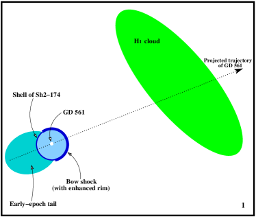
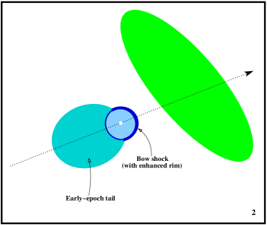
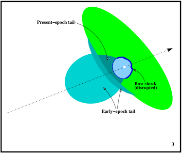
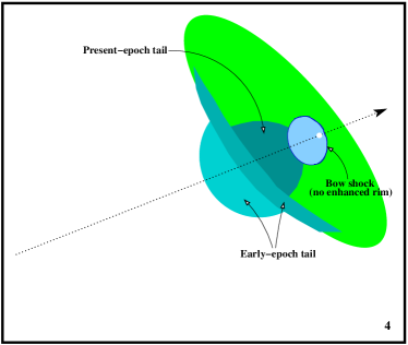
Figure 10: A four-panel cartoon history of the interaction between Sh 2-174 and the ISM. The first two panels show GD 561 (white dot) and Sh 2-174 (circular blue shell) approaching the H I cloud (green ellipse). GD 561 is located at approximately the center of Sh 2-174. The shell is enhanced at the leading edge where a bow shock separates the nebula from the ISM. Material stripped from the leading edge is deposited downstream into a growing tail (cyan ellipse). The tail formed during the pre-cloud interaction is referred to as the early-epoch tail. The third panel shows Sh 2-174 after it has fully entered the cloud. The increased ram pressure at the leading edge has distorted the bow shock, slowed the progression of the upstream portion of Sh 2-174 (relative to GD 561), and increased stripping. The early-epoch tail now has two parts: older material which has not yet encountered the cloud, and younger material accumulating along the edge of the cloud. We also see a present-epoch tail, consisting of material stripped since Sh 2-174 entered the cloud. (Increased tail density is indicated by darker shades of cyan.) The fourth panel represents the present-day picture. GD 561 is close to the leading edge of a flattened Sh 2-174. The bow shock is now less prominent, as much of the leading-edge material has been strewn downstream.

The Faraday rotation revealed in our 1420 MHz polarization images is naturally explained by an interaction between Sh 2-174 and the ISM: we see tail-like structures lagging downstream of Sh 2-174 and a deflection of the ISM magnetic field at the leading edge of Sh 2-174. Indeed, we are catching the likely interaction during a particularly interesting epoch in its history. The projected trajectory of GD 561 indicates that GD 561 and Sh 2-174 entered the H I cloud $\sim$27,000 yr ago (see Figures 8, 9). The increase in ambient density and magnetic field in the cloud, compared to the surrounding ISM, has likely ramped-up the severity of the interaction during this time. Nevertheless, to explain all the observed Faraday-rotation structures in our images, we need to consider the full history of the interaction between Sh 2-174 and the ISM. (Refer to Figure 10 for a pictorial representation of the following discussion.)

Prior to entering the H I cloud, GD 561 and Sh 2-174 were moving through a relatively low-density environment ($n_{H}\sim 0.3$ $\rm{cm}^{-3}$ for the mean ISM at $z\approx 130$ pc, e.g., Dickey & Lockman 1990). Ram-pressure stripping from the head of the bow shock during this earlier epoch produced a tail behind Sh 2-174. We still see this early-epoch tail today. The oldest material continues to move toward the H I cloud, forming what we call region 2. The width of this part of the tail (orthogonal to the projected trajectory) is $\sim$$0.3\arcdeg$, or $\sim$$1.5$ times the major-axis length of Sh 2-174. This is about what we would expect based on simulations (Wareing et al., 2007a). Assuming the tail material in region 2 moves with a speed lagging that of GD 561 by $\gtrsim$15 km s^-1 (see Wareing et al., 2007c), and taking the separation between the eastern edge of region 2 and the present position of GD 561 as the maximum extent of the tail ($3.1\pm 0.9$ pc at $\rm{d}=415\pm 120$ pc), we estimate a lifetime for the PN-ISM interaction $\lesssim$$(2.0\pm 0.3)\times 10^{5}$ yr (where the uncertainty arises from the proper-motion uncertainty for GD 561 given in Table THE EMISSION NEBULA Sh 2-174: A RADIO INVESTIGATION OF THE SURROUNDING REGION). A direct measurement of the velocity of the tail material in region 2 would further constrain this estimate.

Newer material in the early-epoch tail, i.e., material stripped more recently than that seen in region 2, is responsible for the arms of the $S$-shaped structure. As (ionized) tail material approaches the H I cloud, it encounters a rapidly increasing magnetic pressure ($P_{B}=B^{2}/8\pi$) along the trajectory of GD 561, and is deflected into a likely turbulent flow parallel to the cloud’s magnetic field. The LOS component of the cloud’s field broadens the depth of the tail, while the on-sky component broadens the width. Since the arms of the $S$-shaped structure align precisely with the edge of the cloud, we infer that the cloud’s on-sky field component has a position angle very similar to the cloud’s major axis ($\sim$$45\arcdeg$, east of north). The higher mean RM found for the arms compared to region 2 ($-16\pm 5$ $\rm{rad}\,\rm{m}^{-2}$ vs. $-6\pm 2$ $\rm{rad}\,\rm{m}^{-2}$) is not surprising, since the arms have a higher LOS field, longer path length, and likely higher electron density (as tail material accumulates). Differences in the appearance of the north and south arms may arise due to a north-to-south gradient in the cloud’s magnetic-field strength (perhaps matching the observed hydrogen-density gradient). In particular, a weaker field in the south could allow material to spread more easily across field lines, yielding a wider arm with lower mean density.

When Sh 2-174 entered the cloud, the ram pressure of the ISM at its leading edge ($P_{\rm ram}=\rho_{\rm{ISM}}v^{2}_{\rm{S}}$) increased by a factor $\sim$10 (compare $n_{H}\sim 0.3$ $\rm{cm}^{-3}$ outside the cloud to $n_{H}\sim 3$ $\rm{cm}^{-3}$ for the central ridge of the cloud). (The magnetic pressure is much lower than the ram pressure, even for a compressed cloud field at the leading edge of Sh 2-174.) The result was likely a factor $\sim$3 decrease in the forward speed of Sh 2-174, as the nebula found a new pressure balance (viz. $\rho_{w}v^{2}_{w}=\rho_{\rm{ISM}}v^{2}_{\rm{S}}$), and an increased disruption of the bow shock. Over $\sim$20,000 yr (allowing Sh 2-174 to first fully enter the cloud), a factor $\sim$3 difference between the speeds of GD 561 and Sh 2-174 amounts to an angular separation (at $\rm{d}=415\pm 120$ pc) of $0.07\arcdeg\pm 0.02\arcdeg$. This is consistent with the observed separation at present between GD 561 and the center of the optical (i.e., combined R-band and B-band) nebula. As for the bow shock, the increased disruption led to increased and more violent stripping. This in turn led to a denser and more turbulent tail (Wareing et al., 2007a). We see this present-epoch tail as the wide bridge of the $S$-shaped structure. The large fluctuations in RM throughout most of the bridge are consistent with tail turbulence in the form of vortices (e.g., Wareing, Zijlstra, & O’Brien, 2007b). Region 4 along the projected trajectory of GD 561 has relatively low turbulence compared to its surroundings in the bridge. This is not unexpected, as some simulations show a “quiet” zone in the tail immediately behind the interacting PN (e.g., Wareing et al., 2007a). Also, region 4 is offset slightly north of the center of the bridge; i.e., the present-epoch tail extends farther south of the projected path of Sh 2-174 than it does north. This is reasonable, since the ambient cloud, which surrounds and (somewhat) confines the tail, decreases in density north-to-south.

Can the trajectory of GD 561 account for the deflection of the ambient magnetic field from into-the-sky east of Sh 2-174 to out-of-the-sky immediately west of Sh 2-174? The orientation and RMs for the $S$-shaped structure indicate that the ambient field in the cloud has an on-sky component oriented approximately northeast-southwest and a LOS component directed into the sky. In contrast, the space velocity of GD 561 (and Sh 2-174) has an on-sky component directed south-southeast-to-north-northwest and (smaller) LOS component directed out-of the sky. Thus, Sh 2-174 intersects the ambient field at nearly a right angle. Such an intersection should yield a maximum deflection (e.g., Soker & Dgani, 1997). Furthermore, since Sh 2-174 has a velocity component out of the sky, it seems natural that sightlines near the leading edge of Sh 2-174 (region 7 and the westernmost portion of region 6) reveal a small out-of-the-sky field component. Full magnetohydrodynamic simulations are needed in order to better judge the observed behavior of the ISM field during the PN-ISM interaction.

5.6 Resolving Discrepancies with the PN Designation

Our radio results for Sh 2-174 favor an interacting PN interpretation over a Strömgren-zone interpretation. If an interacting PN is indeed the correct interpretation, then Sh 2-174 is in the late stages of an interaction with an H I cloud. As a result, some of the usual observational markers for interacting PNe may be muddled or missing. For example, Sh 2-174 does not have a distinct bow shock. This fact should not be considered surprising, as much of the nebular material originally at the leading edge of the interaction has been strewn downstream into the tail. The R-band cleft-hoof structure may correspond to material still moving downstream toward the tail. The relatively narrow widths of the emission lines (Madsen et al., 2006) and the radial velocity offset between the ionized gas and GD 561 (Frew, 2008) are also peculiarities for Sh 2-174. However, these too can be explained by the interaction between Sh 2-174 and the cloud: the expansion of the PN shell has been halted at the leading edge and restricted elsewhere, and the overall motion of Sh 2-174 has been slowed in the cloud by a factor $\sim$3 compared to GD 561.

If GD 561 evolved via the standard AGB route, its low mass (see Table THE EMISSION NEBULA Sh 2-174: A RADIO INVESTIGATION OF THE SURROUNDING REGION) implies a post-AGB age $>$$10^{6}$ yr (Blöcker, 1995). This is a factor $>$5 times larger than the interaction timescale we estimate for Sh 2-174. The age gap is similarly problematic if we consider a post-early-AGB evolution; i.e., evolution following the early termination of the AGB stage (Dorman, Rood, & O’Connell 1993; Blöcker 1995). However, if GD 561 evolved via a red-giant-branch (RGB) route, its estimated (post-RGB) age is $\sim$$10^{5}$ yr (Driebe et al., 1998). No observed PNe have been unambiguously identified as post-RGB objects (e.g., De Marco, 2009; Hall et al., 2013), but RGB remnants, i.e., helium white dwarfs, are an expected product of close binary evolution and are estimated to make-up $\sim$4% of PN central stars (Nie, Wood, & Nicholls 2012; De Marco et al. 2013). Though Good et al. (2005) find no evidence of binarity in GD 561’s radial velocity, and there is no evidence of an infrared excess for GD 561 (see Zacharias et al., 2013), the existence of a companion cannot be excluded. On account of our radio results for Sh 2-174, it is perhaps reasonable to include the post-RGB scenario in PN-ISM interaction simulations.

5.7 Origin of the $I$-Emission Plateau

Our 1420 MHz $I$ image reveals a low-surface-brightness plateau which appears to emanate from the $I$-emission halo around Sh 2-174 and run $0.30\arcdeg\pm 0.05\arcdeg$ southeast from edge of the H I cloud (see Figure 9). One possible explanation is that the plateau traces the extent to which ionizing photons from GD 561 penetrate the surrounding ISM, after escaping the eastern boundary of the H I cloud. To evaluate this, we consider the electron density in the plateau. The mean brightness temperature over the plateau is $T_{b}=0.045\pm 0.004$ K. Assuming $T_{e}=10000\pm 2000$ K, we estimate a mean EM for the plateau $29\pm 4$ $\rm{cm}^{-6}$ pc. Now, using an angle-equivalent path length $0.5\arcdeg\pm 0.2\arcdeg$ (which translates at $\rm{d}=415\pm 120$ pc to a physical path length $3.6\pm 1.8$ pc), we derive a mean electron density for the plateau $n_{e}=2.8\pm 0.7$ $\rm{cm}^{-3}$. This is much larger than the expected $n_{H}\sim 0.3$ $\rm{cm}^{-3}$ outside the cloud.

Another possibility is that the plateau was formed by an outflow of ionized material from the H I cloud. Sh 2-174 entered the cloud $\sim$27,000 yr ago, ionizing (via GD 561) ambient material and depositing additional ionized material in its wake. The thermal pressure in this part of the cloud increased correspondingly ($P_{\rm th}=nkT$), and the approximate pressure balance between the cloud and surrounding ISM, particularly at the boundary behind Sh 2-174, was broken. To cover $0.30\arcdeg\pm 0.05\arcdeg$ ($2.2\pm 0.7$ pc at $\rm{d}=415\pm 120$ pc) in $\sim$27,000 yr, the resulting outflow speed must be $80\pm 30$ km s^-1. This is $\sim$2 times higher than that seen elsewhere for outflows produced by H II regions breaching the boundary of a confining cloud (e.g., Depree et al., 1994). We can account for most (or perhaps all) of the difference by increasing the flow time. Given the large extent of the GD 561 Strömgren zone in the low-density ISM, it is quite plausible that the outflow started well before Sh 2-174 intercepted the cloud. A direct measurement of the motion of the ionized material in the plateau is necessary to fairly evaluate the outflow model.

Is it surprising that we observe no discernible Faraday rotation on the $I$-emission plateau (outside its superposition with the bridge of the $S$-shaped structure)? In short, no. Thermal emission is proportional to the square of the electron density, while Faraday rotation is proportional to the product of electron density and LOS magnetic field. The electron density in the plateau ($n_{e}=2.8\pm 0.7$ $\rm{cm}^{-3}$) is not high enough, when combined with the relatively low LOS field away from the H I cloud, to rotate the polarization angle of the diffuse background emission by (an observable) $\gtrsim$$3\arcdeg$.

6 CONCLUSIONS

Here we give a summary of our results and conclusions:

1. We have presented 1420 MHz polarization, 1420 MHz total intensity ($I$), and neutral hydrogen (H I) images of the region around Sh 2-174. A superposition of the images shows a physical interconnection between the ionized and neutral structures.

2. The H I images indicate that Sh 2-174 sits presently at the center of an H I cloud. The cloud is $\sim$$1.2\arcdeg$-long and $\sim$$0.4\arcdeg$-wide, and oriented approximately northeast-southwest. Assuming the cloud is optically thin at 21 cm, we estimate a peak neutral hydrogen density $n_{H}=4\pm 2$ $\rm{cm}^{-3}$.

3. The $I$ image reveals thermal emission peaks coincident with the Sh 2-174 R-band emission. We estimate electron densities in the peaks $n_{e}=11\pm 3$ $\rm{cm}^{-3}$. The $I$ image also reveals a low-surface-brightness “halo” around Sh 2-174, and a low-surface-brightness “plateau” running $0.30\arcdeg\pm 0.05\arcdeg$ southeast from the edge of the H I cloud.

4. The polarization images reveal a high-contrast Faraday-rotation structure oriented approximately northeast-southwest and merging at its midpoint with the downstream edge of Sh 2-174. The “arms” of this structure run precisely along the eastern edge of the H I cloud. The polarization images also reveal lower-contrast Faraday-rotation structures along the projected trajectory of GD 561.

5. Our RM analysis indicates that the ISM magnetic field around Sh 2-174 is generally directed into the sky, but deflected at the leading edge of Sh 2-174 such that we find a small out-of-the-sky component at approximately the position of GD 561. We estimate for the Faraday rotation immediately behind Sh 2-174 $\rm{RM}=-44\pm 5$ $\rm{rad}\,\rm{m}^{-2}$. Combining this with an estimate of the electron density behind Sh 2-174, we derive a LOS field component $B_{\|}=8\pm 2$ $\mu\rm{G}$. If this value is representative of the ambient field in the H I cloud, and the field lies as much in the plane of the sky as along the LOS, we estimate a total cloud field $B=11\pm 3$ $\mu\rm{G}$. This estimate is consistent with the statistical mean for diffuse H I sheets and filaments.

6. Our radio results are inconsistent with a Strömgren-zone interpretation for Sh 2-174: we see a mean electron density for Sh 2-174 ($n_{e}=8\pm 2$ $\rm{cm}^{-3}$) that is a factor $\sim$2 higher than the peak hydrogen density in the H I cloud, prominent Faraday-rotation structures downstream of Sh 2-174, and a deflected magnetic field at the leading edge of Sh 2-174. On the other hand, our radio results are consistent with a PN-ISM interaction.

7. Our space-velocity analysis for GD 561 indicates that GD 561 and Sh 2-174 entered the H I cloud $\sim$27,000 yr ago. The increased severity of the PN-ISM interaction in this time has likely led to a factor $\sim$3 decrease in the forward speed of Sh 2-174 and an increased disruption of the bow shock.

8. The transition from outside to inside the H I cloud explains the overall shape of the high-contrast Faraday-rotation structure: The arms of the structure likely represent an early-epoch tail; i.e., material stripped before Sh 2-174 reached the cloud, and now spread-out along the cloud’s edge. The broad mid-region of the structure represents the present-epoch tail; i.e., material stripped since Sh 2-174 entered the cloud, and now sitting immediately behind Sh 2-174.

9. We estimate a PN-ISM interaction timescale $\lesssim$$2.0\times 10^{5}$ yr, consistent with a post-RGB evolutionary path for the low-mass GD 561. We suggest that the post-RGB scenario be added to simulations of the PN-ISM interaction.

10. Even though Sh 2-174 itself is not a Strömgren zone, the $I$-emission halo surrounding Sh 2-174 likely does correspond to the GD 561 Strömgren zone: the extent of the halo is largest where the H I cloud is most diffuse, and smallest where the cloud is most dense. The $I$-emission plateau may be an outflow of material from the ionized cloud region behind Sh 2-174.

Table 1: Properties of GD 561

Parameter		Value		Reference
Equatorial Coordinates (J2000)		23 45 02.254, +80 56 59.72		1
Galactic Coordinates (deg)		120.2169, +18.4302		1
Proper Motion (mas yr-1)		$23.7\pm 2.2$		1
Radial Velocity (km s-1)		$-12.5\pm 0.7$		2
Spectral Classification		DAO		3
$T_{\rm{eff}}$ (K)		$64354\pm 2909$ (Ba), $75627\pm 4953$ (Ly), $74160$ (Ba), $69000$ (Ly+)		4,4,5,6
log $g$ (cm s-2)		$6.94\pm 0.16$ (Ba), $6.64\pm 0.06$ (Ly), $7.16$ (Ba), $6.70$ (Ly+)		4,4,5,6
Mass ($\rm{M}_{\sun}$)		$0.464\pm 0.029$ (Ba), $0.442\pm 0.023$ (Ly), $0.48$ (Ba), $0.40$ (Ly+)		2,2,5,6
Visual Magnitude ($V$)		$14.59$		1
Interstellar Extinction ($E(B-V)$)		$0.089$		4
Distance (pc)		$415\pm 120$

Note. — Units of right ascension are hours, minutes, and seconds, and units of declination are degrees, arcminutes, and arcseconds; mas $\equiv$ milliarcseconds.

References. — 1. UCAC4 (Zacharias et al. 2013);02. Good et al. 2005;03. Bergeron et al. 1994;04. Good et al. 2004;05. Gianninas et al. 2010;06. Ziegler et al. 2012.

Table 2: Faraday-Rotation Model Summary

Region		BPI (K)	BPA	FPI (K)	FPA	RM ($\rm{rad}\,\rm{m}^{-2}$)	Beam Depol.
2		$0.14\pm 0.02$	$-30\arcdeg\pm 10\arcdeg$	$0.13\pm 0.02$	$-15\arcdeg\pm 10\arcdeg$	0$-6\pm 2$	$30\%\pm 5\%$
4		$0.14\pm 0.02$	$-30\arcdeg\pm 10\arcdeg$	$0.13\pm 0.02$	$-15\arcdeg\pm 10\arcdeg$	$-44\pm 5$	$25\%\pm 5\%$
6		$0.14\pm 0.02$	$-30\arcdeg\pm 10\arcdeg$	$0.13\pm 0.02$	$-15\arcdeg\pm 10\arcdeg$	0$-1\pm 2$	$15\%\pm 5\%$
7		$0.14\pm 0.02$	$-30\arcdeg\pm 10\arcdeg$	$0.13\pm 0.02$	$-15\arcdeg\pm 10\arcdeg$	0$+8\pm 2$	0$5\%\pm 5\%$
Arms		$0.14\pm 0.02$	$-30\arcdeg\pm 10\arcdeg$	$0.13\pm 0.02$	$-15\arcdeg\pm 10\arcdeg$	$-16\pm 5$	$50\%\pm 8\%$

Note. — BPI, FPI $\equiv$ background and foreground polarized intensity, respectively; BPA, FPA $\equiv$ background and foreground polarization angle, respectively.

References

- Acker & Stenholm (1990) Acker, A., & Stenholm, B. 1990, A&AS, 86, 219
- Ali et al. (2013) Ali, A., Ismail, H. A., Snaid, S., & Sabin, L. 2013, A&A, 558, A93
- Ali et al. (2012) Ali, A., Sabin, L., Snaid, S., & Basurah, H. M. 2012, A&A, 541, A98
- Barstow et al. (2005) Barstow, M. A., Bond, H. E., Holberg, J. B., et al. 2005, MNRAS, 362, 1134
- Bergeron et al. (1994) Bergeron, P., Wesemael, F., Beauchamp, A., et al. 1994, ApJ, 432, 305
- Blöcker (1995) Blöcker, T. 1995, A&A, 299, 755
- Boumis et al. (2009) Boumis, P., Meaburn, J., Lloyd, M., & Akras, S. 2009, MNRAS, 396, 1186
- Brown et al. (2003) Brown, J. C., Taylor, A. R., & Jackel, B. J. 2003, ApJS, 145, 213
- Cox et al. (2012) Cox, N. L. J., Kerschbaum, F., van Marle, A.-J., et al. 2012, A&A, 537, A35
- De Marco (2009) De Marco, O. 2009, PASP, 121, 316
- De Marco et al. (2013) De Marco, O., Passy, J.-C., Frew, D. J., Moe, M., & Jacoby, G. H. 2013, MNRAS, 428, 2118
- Depree et al. (1994) Depree, C. G., Goss, W. M., Palmer, P., & Rubin, R. H. 1994, ApJ, 428, 670
- Dickey & Lockman (1990) Dickey, J. M., & Lockman, F. J. 1990, ARA&A, 28, 215
- Dorman et al. (1993) Dorman, B., Rood, R. T., & O’Connell, R. W. 1993, ApJ, 419, 596
- Driebe et al. (1998) Driebe, T., Schönberner, D., Blöcker, T., & Herwig, F. 1998, A&A, 339, 123
- Frew (2008) Frew, D. J. 2008, PhD thesis, Department of Physics, Macquarie University, NSW 2109, Australia
- Frew et al. (2010) Frew, D. J., Madsen, G. J., O’Toole, S. J., & Parker, Q. A. 2010, PASA, 27, 203
- Frew & Parker (2010) Frew, D. J., & Parker, Q. A. 2010, PASA, 27, 129
- Geisbuesch et al. (2014 in prep.) Geisbuesch, J., Landecker, T. L., Kothes, R., & Gaensler, B, M. 2014 in prep., ApJ
- Gianninas et al. (2010) Gianninas, A., Bergeron, P., Dupuis, J., & Ruiz, M. T. 2010, ApJ, 720, 581
- Good et al. (2005) Good, S. A., Barstow, M. A., Burleigh, M. R., Dobbie, P. D., & Holberg, J. B. 2005, MNRAS, 364, 1082
- Good et al. (2004) Good, S. A., Barstow, M. A., Holberg, J. B., et al. 2004, MNRAS, 355, 1031
- Gray et al. (1999) Gray, A. D., Landecker, T. L., Dewdney, P. E., et al. 1999, ApJ, 514, 221
- Hall et al. (2013) Hall, P. D., Tout, C. A., Izzard, R. G., & Keller, D. 2013, MNRAS, 435, 2048
- Haverkorn et al. (2004) Haverkorn, M., Katgert, P., & de Bruyn, A. G. 2004, A&A, 427, 549
- Heiles (1996) Heiles, C. 1996, in Astronomical Society of the Pacific Conference Series, Vol. 97, Polarimetry of the Interstellar Medium, ed. W. G. Roberge & D. C. B. Whittet, 457
- Heiles & Troland (2005) Heiles, C., & Troland, T. H. 2005, ApJ, 624, 773
- Heithausen et al. (1993) Heithausen, A., Stacy, J. G., de Vries, H. W., Mebold, U., & Thaddeus, P. 1993, A&A, 268, 265
- Higgs et al. (1997) Higgs, L. A., Hoffmann, A. P., & Willis, A. G. 1997, in Astronomical Society of the Pacific Conference Series, Vol. 125, Astronomical Data Analysis Software and Systems VI, ed. G. Hunt & H. Payne, 58
- Ignace (2014) Ignace, R. 2014, ASTRA Proceedings, 1, 1
- Johnson & Soderblom (1987) Johnson, D. R. H., & Soderblom, D. R. 1987, AJ, 93, 864
- Kohoutek (1983) Kohoutek, L. 1983, in IAU Symposium, Vol. 103, Planetary Nebulae, ed. D. R. Flower, 17–29
- Landecker et al. (2000) Landecker, T. L., Dewdney, P. E., Burgess, T. A., et al. 2000, A&AS, 145, 509
- Landecker et al. (2010) Landecker, T. L., Reich, W., Reid, R. I., et al. 2010, A&A, 520, A80
- Lynds (1965) Lynds, B. T. 1965, ApJS, 12, 163
- Madsen et al. (2006) Madsen, G. J., Frew, D. J., Parker, Q. A., Reynolds, R. J., & Haffner, L. M. 2006, in IAU Symposium, Vol. 234, Planetary Nebulae in our Galaxy and Beyond, ed. M. J. Barlow & R. H. Méndez, 455–456
- McCullough & Benjamin (2001) McCullough, P. R., & Benjamin, R. A. 2001, AJ, 122, 1500
- Napiwotzki (2001) Napiwotzki, R. 2001, A&A, 367, 973
- Napiwotzki & Schönberner (1993) Napiwotzki, R., & Schönberner, D. 1993, in IAU Symposium, Vol. 155, Planetary Nebulae, ed. R. Weinberger & A. Acker, 495
- Nicholls et al. (2012) Nicholls, D. C., Dopita, M. A., & Sutherland, R. S. 2012, ApJ, 752, 148
- Nie et al. (2012) Nie, J. D., Wood, P. R., & Nicholls, C. P. 2012, MNRAS, 423, 2764
- Osterbrock & Ferland (2006) Osterbrock, D. E., & Ferland, G. J. 2006, Astrophysics of Gaseous Nebulae and Active Galactic Nuclei (2nd ed.; Sausalito, CA: University Science Books)
- Parker et al. (2006) Parker, Q. A., Acker, A., Frew, D. J., et al. 2006, MNRAS, 373, 79
- Ransom et al. (2010) Ransom, R. R., Kothes, R., Wolleben, M., & Landecker, T. L. 2010, ApJ, 724, 946
- Ransom et al. (2008) Ransom, R. R., Uyanıker, B., Kothes, R., & Landecker, T. L. 2008, ApJ, 684, 1009
- Reich (1982) Reich, W. 1982, A&AS, 48, 219
- Reich et al. (2004) Reich, W., Fürst, E., Reich, P., et al. 2004, in The Magnetized Interstellar Medium, ed. Uyanıker, B. and Reich, W. and Wielebinski, R., 45–50
- Reid et al. (2008) Reid, R. I., Gray, A. D., Landecker, T. L., & Willis, A. G. 2008, Radio Science, 43, 2008
- Savage et al. (2013) Savage, A. H., Spangler, S. R., & Fischer, P. D. 2013, ApJ, 765, 42
- Schönrich et al. (2010) Schönrich, R., Binney, J., & Dehnen, W. 2010, MNRAS, 403, 1829
- Sembach et al. (2000) Sembach, K. R., Howk, J. C., Ryans, R. S. I., & Keenan, F. P. 2000, ApJ, 528, 310
- Sharpless (1959) Sharpless, S. 1959, ApJS, 4, 257
- Simmons & Stewart (1985) Simmons, J. F. L., & Stewart, B. G. 1985, A&A, 142, 100
- Soker & Dgani (1997) Soker, N., & Dgani, R. 1997, ApJ, 484, 277
- Stil et al. (2006) Stil, J. M., Lockman, F. J., Taylor, A. R., et al. 2006, ApJ, 637, 366
- Sun et al. (2007) Sun, X. H., Han, J. L., Reich, W., et al. 2007, A&A, 463, 993
- Sun & Reich (2009) Sun, X. H., & Reich, W. 2009, A&A, 507, 1087
- Sun et al. (2008) Sun, X. H., Reich, W., Waelkens, A., & Enßlin, T. A. 2008, A&A, 477, 573
- Taylor et al. (2003) Taylor, A. R., Gibson, S. J., Peracaula, M., et al. 2003, AJ, 125, 3145
- Tweedy & Kwitter (1996) Tweedy, R. W., & Kwitter, K. B. 1996, ApJS, 107, 255
- Tweedy & Napiwotzki (1994) Tweedy, R. W., & Napiwotzki, R. 1994, AJ, 108, 978
- Uyanıker et al. (2003) Uyanıker, B., Landecker, T. L., Gray, A. D., & Kothes, R. 2003, ApJ, 585, 785
- Wareing et al. (2006a) Wareing, C. J., O’Brien, T. J., Zijlstra, A. A., et al. 2006a, MNRAS, 366, 387
- Wareing et al. (2007a) Wareing, C. J., Zijlstra, A. A., & O’Brien, T. J. 2007a, MNRAS, 382, 1233
- Wareing et al. (2007b) —. 2007b, ApJ, 660, L129
- Wareing et al. (2007c) Wareing, C. J., Zijlstra, A. A., O’Brien, T. J., & Seibert, M. 2007c, ApJ, 670, L125
- Wareing et al. (2006b) Wareing, C. J., Zijlstra, A. A., Speck, A. K., et al. 2006b, MNRAS, 372, L63
- Wilson et al. (2009) Wilson, T. L., Rohlfs, K., & Hüttemeister, S. 2009, Tools of Radio Astronomy (5th ed.; Berlin, Germany: Springer-Verlag)
- Wolleben et al. (2006) Wolleben, M., Landecker, T. L., Reich, W., & Wielebinski, R. 2006, A&A, 448, 411
- Wolleben & Reich (2004) Wolleben, M., & Reich, W. 2004, A&A, 427, 537
- Xilouris et al. (1996) Xilouris, K. M., Papamastorakis, J., Paleologou, E., & Terzian, Y. 1996, A&A, 310, 603
- Zacharias et al. (2013) Zacharias, N., Finch, C. T., Girard, T. M., et al. 2013, AJ, 145, 44
- Ziegler et al. (2012) Ziegler, M., Rauch, T., Werner, K., & Kruk, J. W. 2012, in IAU Symposium, Vol. 283, IAU Symposium, 211–214