Analysis of the Diffuse Domain Method for second order elliptic boundary value problems
Abstract.
The diffuse domain method for partial differential equations on complicated geometries recently received strong attention in particular from practitioners, but many fundamental issues in the analysis are still widely open. In this paper we study the diffuse domain method for approximating second order elliptic boundary value problems posed on bounded domains, and show convergence and rates of the approximations generated by the diffuse domain method to the solution of the original second order problem when complemented by Robin, Dirichlet or Neumann conditions.
The main idea of the diffuse domain method is to relax these boundary conditions by introducing a family of phase-field functions such that the variational integrals of the original problem are replaced by a weighted average of integrals of perturbed domains. From an functional analytic point of view, the phase-field functions naturally lead to weighted Sobolev spaces for which we present trace and embedding results as well as various type of Poincaré inequalities with constants independent of the domain perturbations. Our convergence analysis is carried out in such spaces as well, but allows to draw conclusions also about unweighted norms applied to restrictions on the original domain. Our convergence results are supported by numerical examples.
+ Cells in Motion Cluster of Excellence, University of Münster.
∗ Dept. of Mathematical Sciences and Technology, Norwegian University of Life Sciences
∘ Corresponding author
Email: burger,schlottbom@uni-muenster.de, ole.elvetun@nmbu.no
Keywords: diffuse domain method, weighted Sobolev spaces, domain perturbations, elliptic boundary value problems
AMS Subject Classification: 35J20 35J70 46E35 65N85
1. Introduction
This paper considers the approximation properties of the diffuse domain method (also called diffuse interface method, cf. [24, 33]) when applied to linear second order elliptic equations of the form
| (1) |
complemented by suitable boundary conditions on a sufficiently smooth domain . We focus on Neumann, Robin and Dirichlet boundary conditions, i.e. either
| (2) | ||||
| (3) |
For solving equations of the above type we will employ variational methods. Roughly speaking, for instance (1)–(2) is reformulated as follows: Find such that for all suitable test functions
| (4) |
In many applications the domain , the boundary (or equally well some interface inside the domain) is not known exactly or its geometry is complicated making a proper approximation of the integrals difficult or expensive [2, 13, 16, 29, 32, 35]. In addition to the methods used in the aforementioned references, let us point to further literature dealing with methods to handle these type of difficulties; for instance the immersed boundary method [31], the immersed interface method [23], the fictitious domain method [15], the unfitted finite element method [5], the finite cell method [30], unfitted discontinuous Galerkin methods [6], composite finite elements [19, 25]; let us also refer to these papers for further links to literature and applications. In this work we will focus on the diffuse domain method, see for instance [24].
The diffuse domain method relies on the fact that the domain can be described by its oriented distance function , . As one can easily see, we have . In order to relax the sharp interface condition , let us introduce for small and being a sigmoidal function, i.e. non-decreasing with for . As tends to zero, converges to the sign function, and hence the phase-field function formally converges to the indicator function of . The key idea to approximate the integrals in (4) is a weighted averaging of the integrals over instead of integrating over the original domain only (and similar for boundary integrals). Since approximates a concentrated distribution at zero, we expect
where we have used the substitution in the last step. Now the layer cake-representation can further be used for given integrable to rewrite
By an analogous computation we obtain for the boundary integral
which can be simplified via the co-area formula to
Here, is a domain with “simple” geometry, i.e. a geometry which can be easily approximated. Based on this motivation we shall define the following diffuse volume and surface integrals
| (5) |
Using this approximation in (4) leads us to the following variational problem: Find such that for all suitable test functions
| (6) |
Under the usual assumptions on , and , the bilinear form on the left-hand side of (6) is well-defined on the weighted Sobolev space , which is the closure of smooth functions with finite (semi-) norm
The main point of the present manuscript is to estimate the error between the solution of (4) and the solution of (6). Our key results are the following two theorems, the first treating the low regularity case and the second giving optimal rates under full regularity:
Theorem 1.1.
Theorem 1.2.
In addition to the assumptions of Theorem 1.1 let be of class , and let . Then there exists a constant independent of such that
Let us mention that the case is allowed here and corresponds to Neumann boundary conditions. The index in Theorem 1.1 is related to regularity of , see [18, 26] and Section 6.1 below. In order to prove the theorems, we need a few technical ingredients. As is obvious from the above discussion, we have to deal with a family of weighted Sobolev spaces parametrized by . For certain choices of , we observe that the weight is proportional to a power of a distance function near , see (12) below. For this type of weights and fixed many results have been established in literature; see for instance [20, 21, 27, 28] and more generally [36]. Since we are dealing with a family of spaces corresponding to a family of weights , we are particularly interested in the behavior of the weighted spaces when changes. We will present trace theorems, embedding theorems and Poincaré inequalities with constants independent of , which turn out to be indispensable tools for the analysis of (6), and which we think might be of interest in their own, see Section 4. In order to prove these statements, we have to revise and adapt the classical proofs of [28] and combine them with arguments recently used in the context of shape optimization; see [3, 8, 11] for such arguments applied to unweighted Sobolev spaces.
A further necessary ingredient to obtain the error estimates of Theorem 1.1 and Theorem 1.2 are rigorous error estimates for the approximations (5) in terms of and the regularity of the integrands. A consequence of our results is that for
see Theorem 5.1. Assuming and in , we can exploit the special averaging procedure in the derivation of the diffuse integrals in a crucial way to obtain the improved estimate
cf. Theorem 5.2. Concerning Robin boundary values, let us mention recent formal result obtained by asymptotic analysis stating an -convergence rate for the error of [22]. Using a problem adapted norm we also obtain a rate . For two-dimensional problems and under reasonable assumptions on this problem adapted norm, which we however cannot verify for our problem, we also arrive at a -convergence rate . The latter is well confirmed by numerical results.
Concerning Dirichlet boundary values, the corresponding convergence rate only yields the half order compared to the Robin boundary values. Hence in the setting of Theorem 1.1, but with (3) instead of (2), we obtain
and accordingly, in the setting of Theorem 1.2 with (3) in place of (2), we obtain
In the best case, using the problem adapted norm, we can show a rate . This complies with recent results in literature, which were obtained for one-dimensional problems or numerically [14, 34].
The outline of the manuscript is as follows. In Section 2 we discuss the geometry of and certain perturbations of it. Section 3 introduces weighted Lebesgue and Sobolev spaces together with some basic properties. A more detailed study of weighted Sobolev spaces is presented in Section 4. Here we present a trace and an embedding theorem for weighted Sobolev spaces and we show that the corresponding estimates are stable with respect to . Moreover, we prove Poincaré and Poincaré-Friedrichs inequalities for these spaces again with constants independent of . Approximation properties of the diffuse integrals are presented in Section 5. The volume integrals are investigated in Section 5.1, and corresponding results for the diffuse boundary integral are subsequently shown in Section 5.2. Section 6 deals with the approximation of elliptic equations by the diffuse domain method for Robin, Dirichlet and Neumann type boundary values, and proofs of Theorem 1.1 and Theorem 1.2 are given. Our results are supported by numerical results which are presented in Section 7. We conclude in Section 8 and discuss briefly some open questions.
2. Some geometric preliminaries
2.1. Domain
Throughout the manuscript we assume that is a domain with boundary. Associated to we define its oriented distance function by
Since is of class we have that is in a neighborhood of [11]. For let us define the sublevel sets of as follows
We clearly have the inclusions for all . Moreover, we fix a domain such that . In applications is a domain with a “simple” geometry, for instance a ball or a bounding box.
2.2. The tubular neighborhood
Let us define the -tubular neighborhood of by
| (7) |
Due to regularity of , the projection of onto is unique for sufficiently small, i.e., for each there exists a unique such that [11, Chapter 7, Theorem 3.1, Theorem 8.4]. Here, , , denotes the outward unit normal field which is related to the oriented distance function via the formula . This shows
In the whole manuscript we fix so small such that the just described projection is single-valued. Thus, for each , , and for every , there holds and for every , there holds . Moreover, for some constant independent of
| (8) |
Here, is the -dimensional Lebesgue-measure of and is the -dimensional Hausdorff-measure of .
2.3. Transformations of the geometry
Let . Let us first consider transformations of boundaries . To do so, we introduce a family of transformations defined by . The Jacobian satisfies , with being the identity matrix on and being the Hessian of , and thus,
| (9) |
Decreasing if necessary, there holds and
| (10) |
Denoting by the unit outer normal vector field of , we see that for all by the choice of the tubular neighborhood . Thus, here and in the following, we will just write for the unit outer normal at some . In particular, can be extended to the whole of , and for this extension we have that
particularly, . For , and we then have
| (11) |
Note that for , and hence, for . Here, is the surface element of , i.e.
For the volume transformation , we define by for , and for . Then , and as . Moreover, maps one-to-one onto . We then define the diffeomorphism
Since , the Jacobian of is given by
and as by construction of . We note that .
3. Weighted Sobolev spaces
In order to construct the weighted spaces mentioned in the introduction let us begin with defining another level set function for the domain resembling a sign function smoothed in , namely
where the function is a regularization of the sign function. Hence, if and only if . To be precise, we assume that verifies the following assumptions.
-
(S1)
is Lipschitz continuous, for , and for . Moreover, for all .
-
(S2)
There exist and such that for all
-
(S3)
for all .
(S3) asserts concavity of on and this assumption is only needed in Theorem 5.6 below. Assumption (S2) ensures that that the phase-field function is proportional to on , where is defined as a regularization of the indicator function of as follows
Obviously, we have that , and for with . Let us clarify (S2) in the following. We observe that for . Thus, by (S2) with
| (12) |
Before proceeding, let us give a few examples which may serve as prototypes for .
Example 3.1.
(i) Let for . Obviously (S1) and (S3) are satisfied. Moreover, , and we can choose , and in (S2).
(ii) Let . Thus, and for . Since for , (S3) is satisfied. Moreover, , and (S2) is satisfied for and and .
(iii) Let . Thus, and for . Since for , (S3) is satisfied. Moreover, , and (S2) is satisfied for and and .
Proceeding with the construction of weighted Lebesgue spaces, let us introduce the measure
which is absolutely continuous with respect to the Lebesgue measure. Associated to let us further introduce for the weighted -spaces
For , we set , i.e. is the class of Lebesgue-measurable functions being essentially bounded. In the following we will use also the notation where is an appropriate weight function. The following statement provides some basic relations between the weighted -spaces.
Lemma 3.2.
Let and let . Then , and for every there holds . Moreover,
(i) for we have
(ii) for we have
Proof.
(i) For we obtain
For we have , and on there holds . The fact that yields the assertion.
Associated to the weighted spaces , let us define the weighted Sobolev spaces
with norm
In view of (12), several results of Kufner [21] concerning power-type weights can be applied. This is due to the fact that the proofs of [21] need the power-type property of the weight only in a vicinity of the boundary; in the remaining subset of , say , uniform boundedness away from zero and boundedness of the weight is used, which in turn allows to use results for unweighted spaces. We will employ similar techniques in the next section. We have the following. For , the spaces and are separable Banach spaces [21, Theorem 3.6], and is dense in [21, Theorem 7.2]. In case , the spaces and are Hilbert spaces with obvious definition of the inner product.
4. Properties of Sobolev spaces for diffuse interfaces
In this section we establish basic results for weighted Sobolev spaces for diffuse interfaces which are crucial for the analysis of variational boundary value problems. We particularly investigate the dependence on the parameter . As shown below, our results yield constants independent of , for instance the trace constant or the Poincaré constant in weighted Sobolev spaces, see Theorem 4.2 or Theorem 4.9. These results may be of interest in their own.
4.1. Trace lemma
The following auxiliary lemma is a slight adaptation of [3, Lemma 2.1]. It states that the trace operator for unweighted Sobolev spaces is uniformly bounded for certain perturbations of the domain, and it is the key observation in proving a similar statement also for weighted Sobolev spaces. For convenience of the reader, we sketch a proof.
Lemma 4.1.
Let be sufficiently small. Then there is a constant such that for each and , ,
| (13) |
Proof.
Let be sufficiently small and let . Let us first consider the case . Denote by and the transformations defined in Section 2.3. By a change of variables for and for , it follows that
In view of Section 2.3, as
Denote by a bound for the norm of the trace operator . We then obtain
For the general case , we apply the latter estimate to . We observe that , and, using Young’s inequality, , which concludes the proof. ∎
Theorem 4.2 (Trace lemma).
Let be sufficiently small. Then there exists a constant such that for and for , ,
Proof.
According to the coarea-formula there holds
Since for , we can use (13) to obtain
where we used Fubini’s theorem in the last step. The assertion follows from . ∎
4.2. Embedding theorem
The following embedding theorem uses the representation (12) of the weight near the boundary as a power of the distance function . Let us define the Sobolev conjugate for weighted spaces
| (14) |
We observe that is the “usual” Sobolev conjugate for unweighted Sobolev spaces, see [1], and is strictly decreasing with respect to on .
Theorem 4.3 (Embedding).
Let , and let be the constant from (S2). Then the following embeddings are continuous
Moreover, there exists a constant independent of such that for
| (15) |
The first part of the theorem can be found in [20, Theorem 3], see also [28, Theorem 19.9] for the case . To show that the embedding is independent of , we will give a proof in the spirit of [28]. To do so, we employ the following two lemmata. The first of which uses Sobolev’s embedding theorem on balls and a covering argument, and is similar to the arguments of [28]. The second is a Hardy-inequality-type argument for diffuse interfaces which seems to be new. We let in the following.
Lemma 4.4.
Let and . Furthermore, let such that . Then there exists a constant independent of such that for every
Proof.
We proceed as in [28]. Let . According to the Besicovitch covering theorem, cf. [28, Lemma 18.3], there exists a sequence and an integer depending only on such that
Employing the Sobolev embedding theorem for balls [1], we obtain as in [28, Theorem 18.6]
| (16) |
for all . Note the different powers of the weight on the right-hand side of (16). Assuming, without loss of generality, that and thus , we can bound the right-hand side of (16) as long as and are such that . Hence, by summation over , we obtain the assertion with a constant depending on and the Sobolev embedding constant for the unit ball, but not on . ∎
Lemma 4.5 (Hardy-type inequality).
Let and let . Then there exists a constant independent of such that for every
Proof.
Let . We obtain by using (11), , and one-dimensional integration-by-parts
| (17) |
To treat the first integral in (17), we employ the transformation defined in Section 2.3, i.e.
From , and , and the trace lemma 4.1 we deduce that there exists a constant independent of such that
i.e. . The assertion follows from
and a density argument. ∎
Remark 4.6.
Let us state that the arguments of [21] are based on partition of unity subordinate to where is a finite cover of . Then the Hardy-type argument of the latter proof is applied to which is zero on the boundary of . Hence, the first term in (17) vanishes. However, , and . Thus, the techniques of [21] are not directly applicable as we strive for constants uniformly bounded in terms of .
Proof of Theorem 4.3.
We split the norm into the diffuse interface part and the interior part
From the Sobolev embedding theorem [1], we have that is continuous for each if , and for if . Since and is bounded, we only have to estimate the -norm of on .
First consider the case , . For this choice, the condition is obviously satisfied. Combining Lemma 4.5 and Lemma 4.4 yields
Multiplication of the latter inequality with , taking the th root and using (12), i.e. , further gives,
Summarizing, we have shown that for each there holds
For the general case , we apply the previous results to and . One easily verifies that is equivalent to . Moreover, and . Whence, Hölder’s inequality yields
This together with the identity
yields the assertion. ∎
Remark 4.7.
As already noted, is strictly decreasing with respect to on . Loosely speaking, compared to the unweighted Sobolev embedding, we loose spatial dimensions. For instance, if , we have that for , and for . This fact is intimately related to the Hardy inequality and isoperimetric inequalities, cf. [20] where also counterexamples are given showing that the restriction cannot be improved in general. However, embedding in certain Hölder spaces is possible [20, 28]. Adapting the above proofs it should be possible to show that even in this situation the embedding constants are independent of .
Proposition 4.8 (Compactness).
Let , be the constant in (S2), and let . Then the following embeddings are compact
Proof.
Let and let be bounded; say by a constant . Furthermore denote by the constant of the embedding . Since is complete, we have to show that a subsequence of is Cauchy in . Therefore, let and choose . Since the embedding is compact [1], we can extract a subsequence, again denoted by , which is Cauchy in . Hence, there exists such that for all . Let in the following. Thus, using the triangle inequality, we have that
| (18) |
Since , we obtain by using Hölder’s inequality and the embedding theorem
by choice of . This in combination with (18) shows that is Cauchy in . ∎
The idea of the proof of the previous compactness result can already be found in [28].
4.3. Diffuse Poincaré-Friedrichs inequalities
The last issue concerning basic results in weighted Sobolev spaces are Poincaré-Friedrichs inequalities, which we again want to derive with constants independent of . We start with a quite general result:
Theorem 4.9 (Poincaré-type inequality).
Fix . Assume that is connected for each , and let , be a family of closed cones, i.e. for there holds for all , such that contains only the zero function as a constant function. Then there exists a constant independent of such that
| (19) |
Proof.
Assume (19) is not true. Then there exist sequences with and such that
| (20) |
Since the Bolzano-Weierstraß theorem implies the existence of a such that for a subsequence, relabeled if necessary, as . Hence, for all there exists such that for all . In the following let and . By Hölder’s inequality and the embedding theorem for , we have
| (21) |
Furthermore, since , by Lemma 3.2 (i)
In view of Proposition 4.8, we can therefore extract a subsequence, relabeled if necessary, such that in . Moreover, we deduce from (20) and Lemma 3.2 (i) that
and hence in and . Since is closed and is connected, and on . In view of Lemma 3.2 (ii), we further obtain
This in combination with (21) implies
Since was arbitrary, this is the desired contradiction. ∎
Let us remark that in [8] a similar result has been obtained for unweighted spaces, i.e. a Poincaré inequality with a constant which is independent of certain perturbations of . For illustration of the previous result let us state the “usual” Poincaré and Friedrichs inequality in their weighted form.
Corollary 4.10.
Let , , and let be connected. Then there exists a constant independent of such that
Here is the weighted mean value.
Proof.
Define and use Theorem 4.9. ∎
Corollary 4.11 (Poincaré-Friedrichs-type inequality).
Let , , and let be connected. Then there exists a constant independent of such that for every and there holds
Proof.
Define and use Theorem 4.9. ∎
Remark 4.12.
Remark 4.13.
5. Convergence of diffuse integrals
In the following two subsections we investigate the approximation properties of the diffuse integrals introduced in (5).
5.1. Convergence of diffuse volume integrals
We start with the case of volume integrals, for which we want to estimate the error
between the volume integral and the diffuse volume integral in terms of and . We will provide estimates for the cases and which gives stronger results improved by one order of .
Theorem 5.1.
Let and . Then there exists a constant independent of such that
Moreover, if and , then as .
Proof.
Theorem 5.1 for -functions relies basically on the fact that . This is due to the fact that -functions can have singularities in . Note that in the case we expect no rate of convergence in terms of , and the assumption is stronger than those for . Resorting to -functions we can exploit extensively symmetry of the phase-field function leading to a much stronger result.
Theorem 5.2.
Let , and let for some . Then there exists independent of such that
Proof.
Using a change of variables and Fubini’s theorem, we observe that
Since , we further obtain
Observing that
and splitting the integration over to and and employing a change of variables for the integral over , we further obtain
| (22) |
For the last computation, we used , i.e. . To compare the difference on the right-hand side of the latter equation we use the transformations introduced in Section 2.3, and the transformation formula, namely
The two integrals can be treated separately. Using , and we obtain using Fubini’s theorem and the transformation formula
For the second integral we obtain
| (23) |
which can be seeen with (10) as
Using these estimates we obtain from (22)
Setting , an application of Hölder’s inequality thus yields
Using boundedness of the first integral can be computed explicitly. To treat the second integral, we use Hölder’s inequality for the inner integral which gives
Note, that is a universal constant depending only on , and but not on or which may change from to line. Using , and , we therefore have
Since for , a corresponding transformation yields
where we used that on , and
This yields the assertion. ∎
For sake of completeness, let us state a corresponding approximation result for Hölder continuous function, i.e. we say that , if is continuous on and if
We write .
Lemma 5.3.
Let , and let for some . Then there exists independent of such that
Proof.
It is easy to show the estimates
and
The proof is completed by integration over with similar arguments as in the proof of Theorem 5.2. ∎
5.2. Convergence of diffuse boundary integrals
In this section we investigate the accuracy of the diffuse boundary integral approximation. For this sake consider
In the following we reduce the treatment of to that of from the previous section. Using and the divergence theorem, we see that
Note that, for any , and thus has a trace on . To treat the diffuse boundary integral, we first observe that on . For the definition of see (7). Therefore, integration-by-parts shows that
Notice, that due to there are no boundary integrals. Thus, we have that
Setting , we can use Theorem 5.1, Theorem 5.2 and Lemma 5.3 of the previous section.
Lemma 5.4.
Let be of class and let . Moreover, let for some . Then there exists a constant independent of such that
Lemma 5.5.
Let be of class . Moreover, let for some and . Then there exists a constant independent of such that
The estimate of Lemma 5.5 assumes -regularity of the whole integrand. For our analysis we will also need a slightly different statement:
Theorem 5.6.
Assume is of class , let (S3) hold and let . Furthermore, let satisfy on and let with . Then there exists a constant independent of , and such that for
The higher integrability of improves the first part of the estimate whereas the higher integrability of improves the second part. For the rate is which is optimal for . For we obtain the best possible rate .
Proof.
We start with an inequality for . An application of (11), (9) and Theorem 4.2 yields
| (24) | ||||
with independent of .
Now let , then there exists a constant C such that
| (25) |
This can be seen as follows: By change of variables and application of the fundamental theorem of calculus, we obtain
Repeated application of Hölder’s inequality gives
Using boundedness of and calculating yields the assertion.
We are now in the position to give a proof of the theorem. By setting in (24), we have that
Thus, to prove the theorem, it is sufficient to estimate the second integral on the left-hand side of the latter inequality. Using and , we see that
We treat the two terms on the right-hand side separately. For the first one, we will use (25) with , Hölder’s inequality and which yields
where we have used Lemma 4.1 to treat the term involving and the transformation formula to treat the term involving , see the last lines of the proof of Theorem 5.2. For the second term we first use Hölder’s inequality twice
Then, using (11), we obtain similarly as in the proof of Theorem 5.2
and by (11), (S3), and by Theorem 4.2
The integrals over as well as the ones involving can be treated similarly. Collecting all terms yields the assertion. ∎
Up to now, we have always assumed the boundary data to be regular. For completeness, let us also consider the case only. Then is defined a.e. on , and we can define an extension a.e. on by
| (26) |
Lemma 5.7.
Let and let with , , and . Then there exists a constant independent of such that
with being the extension defined in (26).
Proof.
Using and the transformation formula, we obtain
Thus, using (9), there exists independent of such that
We treat the two integrals on the right-hand side separately. Repeated use of Hölder’s inequality and yields similarly as in the proof of Theorem 5.2
An analogue estimate hold for the integral over . Since, this is the desired estimate for the first integral. The second can be estimated similarly, i.e.
The last term can be estimated using the trace theorem 4.2. ∎
For the sake of completeness, we also state an analog to Lemma 5.3.
Lemma 5.8.
Let be of class for some . Moreover, let for some . Then there exists a constant independent of such that
Proof.
Since , we have . The assertion follows from Lemma 5.3. ∎
6. Diffuse elliptic problems
In this section we investigate three typical second order elliptic boundary value problems. We start with Robin-type problems, which build the basis for further investigations. For rather irregular data, we obtain a weak sublinear convergence result in terms of . Superlinear convergence is achieved by requiring smooth data. In Section 6.2 we treat Dirichlet boundary conditions which can be reduced to the analysis of a Robin problem by means of the well-known penalty method. In Section 6.3 we consider Neumann boundary conditions and establish well-posedness of the diffuse domain method. Apart from the well-posed the convergence results can be derived as in the Robin case.
6.1. Robin boundary conditions
Consider the following second order elliptic equation with Robin-type boundary condition: Find such that
| (27) | ||||
| (28) |
In order to obtain (weak) solutions to (27)–(28), let us consider the following weak formulation: Find such that
| (29) |
with bilinear and linear form
In order to prove well-posedness of the weak form (29) via the Lax-Milgram lemma we make the following assumptions:
-
(C1)
, .
-
(C2)
is a symmetric positive definite matrix, i.e. there exists such that for a.e.
Lemma 6.1.
Let (C1)–(C2) hold. Moreover, let and . Then there exists a unique satisfying (29), and there exists such that
The diffuse approximation of (29) is now: Find such that
| (30) |
where the corresponding bilinear and linear form are given by
Lemma 6.2.
Let (C1)–(C2) hold. Moreover, let and . Then there exists a unique satisfying (30), and there exists independent of such that
Proof.
Denoting by and the corresponding solutions to (29) and (30), respectively, we next want to estimate the error with respect to the -norm which directly implies estimates in the -norm as well. By regularity of , we can assume that is extended to preserving -regularity. Hence, the error satisfies
| (31) |
6.1.1. Sublinear convergence
In order to obtain a first estimate for the error , we estimate the right-hand side of (31) by employing the embedding theorem 4.3. We recall the definitions , see (14), and
which is the norm of as an element of the dual space of .
Lemma 6.3.
Let and . Then there exists a constant independent of such that
Proof.
In order to obtain convergence rates, we need some regularity of .
Lemma 6.4.
Let for some . Then there exists a constant independent of such that
Proof.
Having estimated the errors in right-hand side and bilinear form we can proceed to the main approximation results in this section:
Theorem 6.5.
Remark 6.6.
Remark 6.7.
(i) Assuming and extended by zero to an inspection of the proof of Theorem 5.1 shows that for each
which is due to the embedding and the fact that . This immediately leads to a stronger result in Lemma 6.3 independent of . However, for proving Lemma 6.4, we have to estimate the term
Here, on the one hand, to preserve regularity of , setting on is not possible. On the other hand setting on is not allowed since then (6) is not well-posed anymore.
(ii) If , and , then using the techniques from above, we would obtain the bound
as since the test function is merely . For smooth test functions and and , the right-hand side of (31) is bounded by a constant multiple (depending on , and ) of . This estimate, however, does not lead to -estimates for the error anymore. We will return to these type of estimates in the next section. We also mention that an inspection of several proofs above shows that crucial terms drop out if the involved functions are symmetric with respect to (mirrored along the normal direction). Thus, using symmetric extensions of data and solutions as well as a restriction to a Sobolev space of functions symmetric with respect to could give higher order rates. However, since this does not correspond to the computational practice and would extremely complicate the numerical solution, this seems not of particular practical relevance and hence we do not pursue this direction further.
6.1.2. From linear to quadratic convergence
In literature there exist very recent formal results for the diffuse domain method that state a rate of convergence for the -norm of for the Poisson equation with Robin boundary conditions [22]. To give a precise and rigorous statement of such a better rate we need additional regularity of the domain, the data and the solutions. Furthermore, we resort also to other functions spaces. For a smooth function and we let and define
We let denote the completion of with respect to . Then is a Banach space. Due to the Riesz representation theorem, Corollary 4.11, and assumptions (C1)-(C2) on the coefficients, we see that with equivalent norms. Furthermore, due to Theorem 4.2 we easily see that . For the other direction, we need a solvability result. If for any there exists such that for all and for some constant , then . Let us emphasize that such a result is not known to us for the case ; we refer to [12, 18] for a corresponding result in the unweighted case.
Let us thus start with an error estimate in . For simplicity, we will assume smooth data. It should become clear from the proof how to lower these regularity assumptions.
Theorem 6.8.
Proof.
Due to [17, Thm. 2.4.2.7, Rem. 2.5.1.2] and the smoothness of the data, we have that for any , i.e. by embedding, and is a classical solution to (27)–(28). Therefore, integrating by parts on the right hand side of (31), we deduce that for any the error satisfies
In view of Theorem 5.2 we have the estimates
Since , the remaining terms can be estimated as follows
where we used on and Theorem 5.6. Hence, taking the supremum over all and observing that yields the assertion. ∎
Corollary 6.9.
Let the assumptions of Theorem 6.8 hold true. Then, there exists a constant independent of such that
Proof.
Set in Theorem 6.8. The assertion follows from with equivalent norms. ∎
Remark 6.10.
Setting in Theorem 6.8, we obtain . Let us assume that the norms of and are equivalent (uniform with respect to ). Then continuity of the embedding implies the existence of a constant independent of such that
In particular for , we obtain for any , and for we obtain , thus we recover the formal results of [22].
6.2. Dirichlet boundary conditions
In this section we consider the diffuse domain approximation of second order elliptic equations with Dirichlet boundary conditions: Find such that
| (32) | ||||
| (33) |
In order to obtain (weak) solutions to (32)–(33), let us consider the following weak formulation: Find such that
| (34) |
with bilinear and linear form
Here is the kernel of the trace operator on . The weak form (34) is well-posed under assumptions (C1)–(C2) which is shown by using the Lax-Milgram lemma. It is well-known that the solution to (34) is characterized as the solution of the minimization problem
Using the Lagrange formalism this constrained optimization problem is equivalent to finding a saddle-point of the Lagrangian
| (35) |
Here, is the topological dual space of the -trace space , and denotes the duality pairing between and . The variational characterization of the saddle-point problem is the following: Find such that
| (36) | ||||
| (37) |
We have by definition of the norm on that
which asserts an inf-sup condition for the bilinear form . Well-posedness of the latter saddle-point problem can then be shown by using Brezzi’s splitting theorem [10], cf. [9, Chapter III]. Next, let us introduce a penalized version of (36)–(37) which establishes a connection to elliptic problems with Robin boundary condition discussed in Section 6.1: Let . Find such that
| (38) | ||||
| (39) |
In slight abuse of notation, denotes the inner product on , and is defined as . Here, is the Riesz isomorphism and is given as the trace of the solution to the Neumann problem
We have that
Well-posedness of (38)–(39) can be shown with a penalty version of Brezzi’s splitting theorem, cf. e.g. [9]. In particular is bounded in independent of .
Since depends Lipschitz-continuously on , the error between the solution to (36)–(37) and (38)–(39) is ; for a proof let us refer to [9, Ch. III, Thm 4.11, Cor. 4.15].
Lemma 6.11.
Using with in (39) and adding the resulting equation to (38) yields the following reduced problem: Find such that
This is a weak form of a Robin-type problem with boundary condition on .This method of relaxation of the Dirichlet boundary condition is widely known as the penalty method [4]. Let denote the diffuse approximation to as defined in Section 6.1, i.e. satisfies
| (40) |
for all . Combining the estimates in Lemma 6.11 and Theorem 6.5, we have
| (41) |
for , and . Choosing , , yields
Balancing the exponents on the right-hand side, we obtain the optimal choice . The corresponding estimates are then given by the next theorems:
Theorem 6.12.
Theorem 6.13.
Remark 6.14.
Remark 6.15.
In order to obtain an analogous statement of Theorem 6.8 for the Dirichlet case, we would need an analog of Lemma 6.11 for the -norm. Hence, for illustration let us assume that for . Moreover, by regularity of , we can assume stability of the extension of and to , i.e. . Then, we arrive at the estimate
using and Theorem 6.8. Assuming furthermore that the norms of and are equivalent (uniform with respect to ), and using continuity of the embedding we infer that
In particular for , we obtain for any , and for we obtain . The reader should compare this to the results of [14] where for a rate for any in the -norm is shown. Moreover, in [34] an -rate for Poisson’s equation in three dimensions has been obtained numerically. There, it is also suggested to choose , which complies with our analysis. Let us note however that the diffuse domain method in [34] is somewhat different from ours.
6.3. Neumann boundary conditions
Consider the following second order elliptic equation with Neumann-type boundary condition: Find such that
| (42) | ||||
| (43) |
In order to obtain (weak) solutions to (42)–(43), let us consider the following weak formulation: Find such that
| (44) |
with bilinear and linear form
In view of the usual Poincaré inequality for , the weak form (44) is well-posed under the assumptions (C1)-(C2).
Lemma 6.16.
Let (C1)–(C2) hold. Moreover, let and . Then there exists a unique satisfying (44), and there exists such that
The diffuse approximation of (44) is then: Find such that
| (45) |
where the corresponding bilinear and linear form are given by
Lemma 6.17.
Let (C1)–(C2) hold. Moreover, let and . Then there exists a unique satisfying (30), and there exists independent of such that
Proof.
Continuity of and with respect to the -topology is obvious. Coercivity of on is a direct consequence of the positivity of and the Poincaré inequality, see Corollary 4.10. An application of the Lax-Milgram lemma yields the assertion. ∎
Having established existence of solutions to the Neumann problems, convergence results can now be derived as in the Robin case above when setting . We leave this to the reader. Let us mention that the restriction from to the space is only necessary if . In this case the algebraic condition has to be treated with care in a numerical implementation. We do not want to go into details here, but let us refer the reader to [7]. If otherwise , we could equally well pose (45) in the space and the implementational details are similar to those of the Robin case. We thus will not dwell on the Neumann case in our further discussion.
7. Numerical Results
In the following we report the results of numerical tests related to the above investigations used conformal first order finite elements. Our particular interest here is not the efficient solution of realistic problems, but rather to test the sharpness of error estimates in different situations by computational experiments. In order to have an ”exact“ solution we solve the original problem with sharp interface on a very fine mesh such that the numerical error is negligible. Moreover, in the computation of the diffuse domain solution we make sure that the largest mesh parameter, i.e. , is for all computations smaller than such that the numerical accuracy does not pollute the experimental order of convergence. The error will always be measured in the relative norms
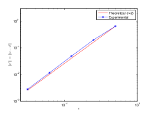
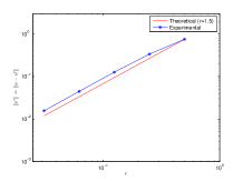
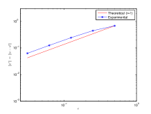
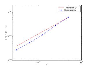
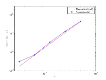
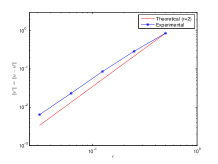
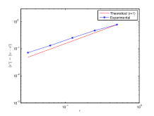
where . We provide several log-log plots of errors vs. , which shall be comparable to the theoretical orders represented by lines in those plots, see Figure 1, 3, 6 and 8. Since the constants in the estimates cannot be made explicit, we have to fix one value and hence decide to plot the theoretical rates in all log-log plots such that they coincide with the experimental rates for the largest value of , see Figure 1, 3, 6 and 8.
For most simulations (Case A-D below) we work with the domain , which obviously satisfies all regularity requirements. The mesh representation of this domain consists of vertices. The mesh representation of the domain is simply a scaling of the mesh representation of with . Finally we present an example with the domain , i.e. the unit square (Case E), which indicates that the same rates still hold for piecewise smooth domains. In all test cases we use the function from Example 3.1 (i).
7.1. Case A: Robin BC with smooth parameters
In our first simulations, we consider the boundary value problem (27)-(28), with the smooth parameters
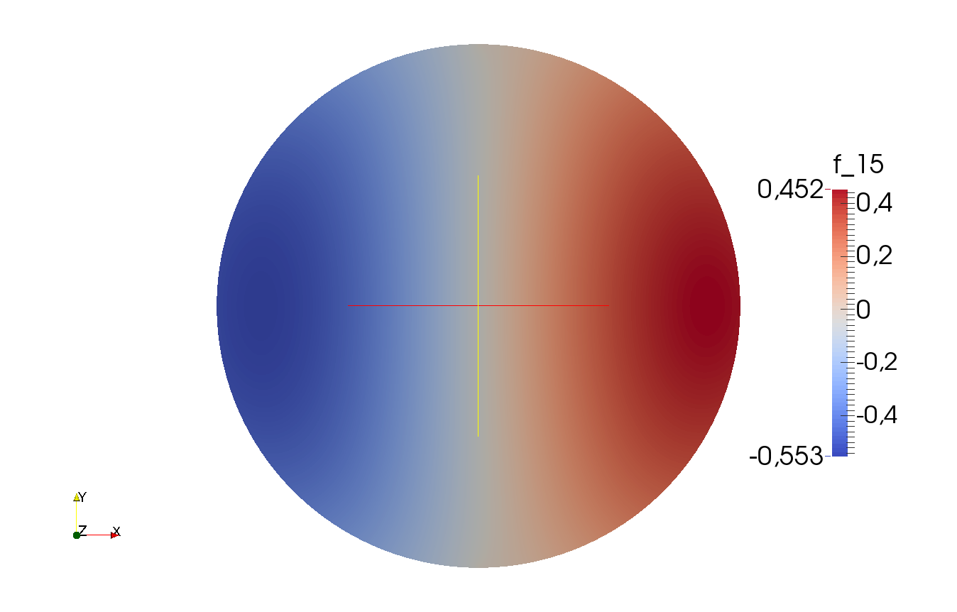
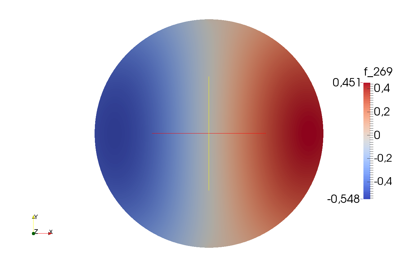
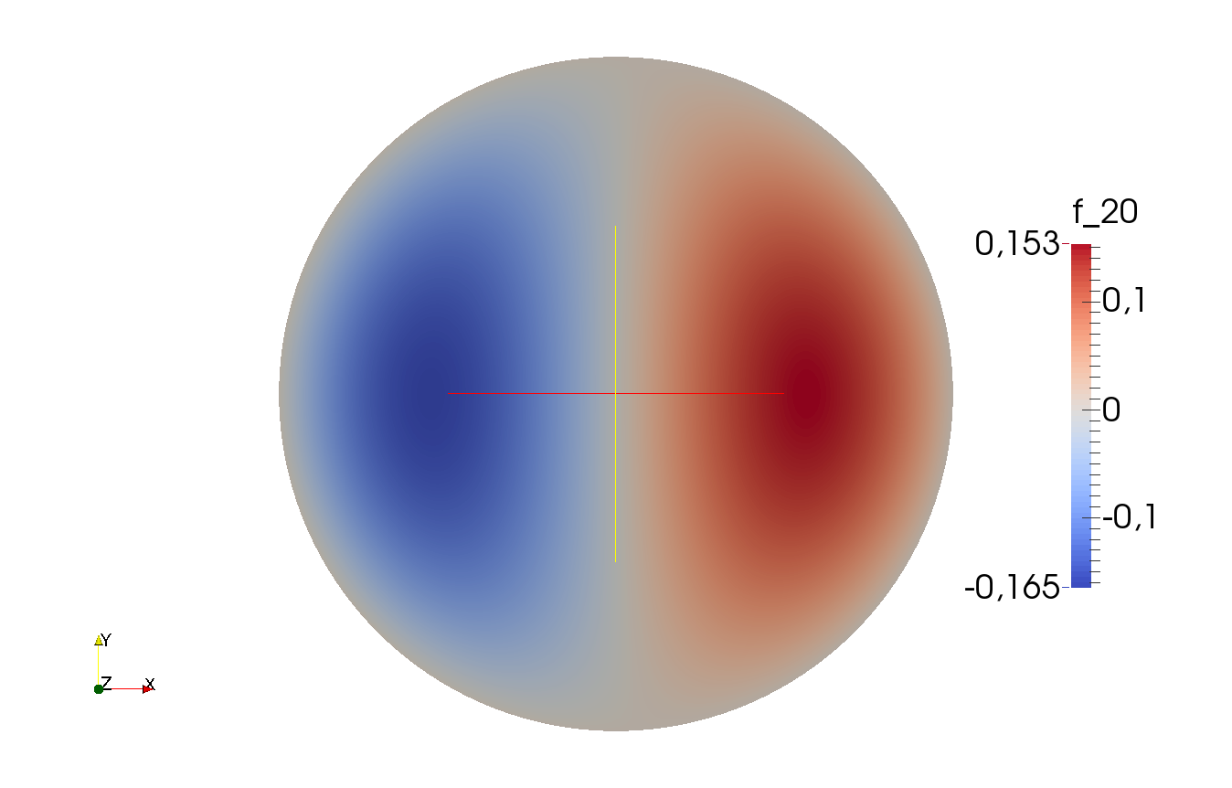
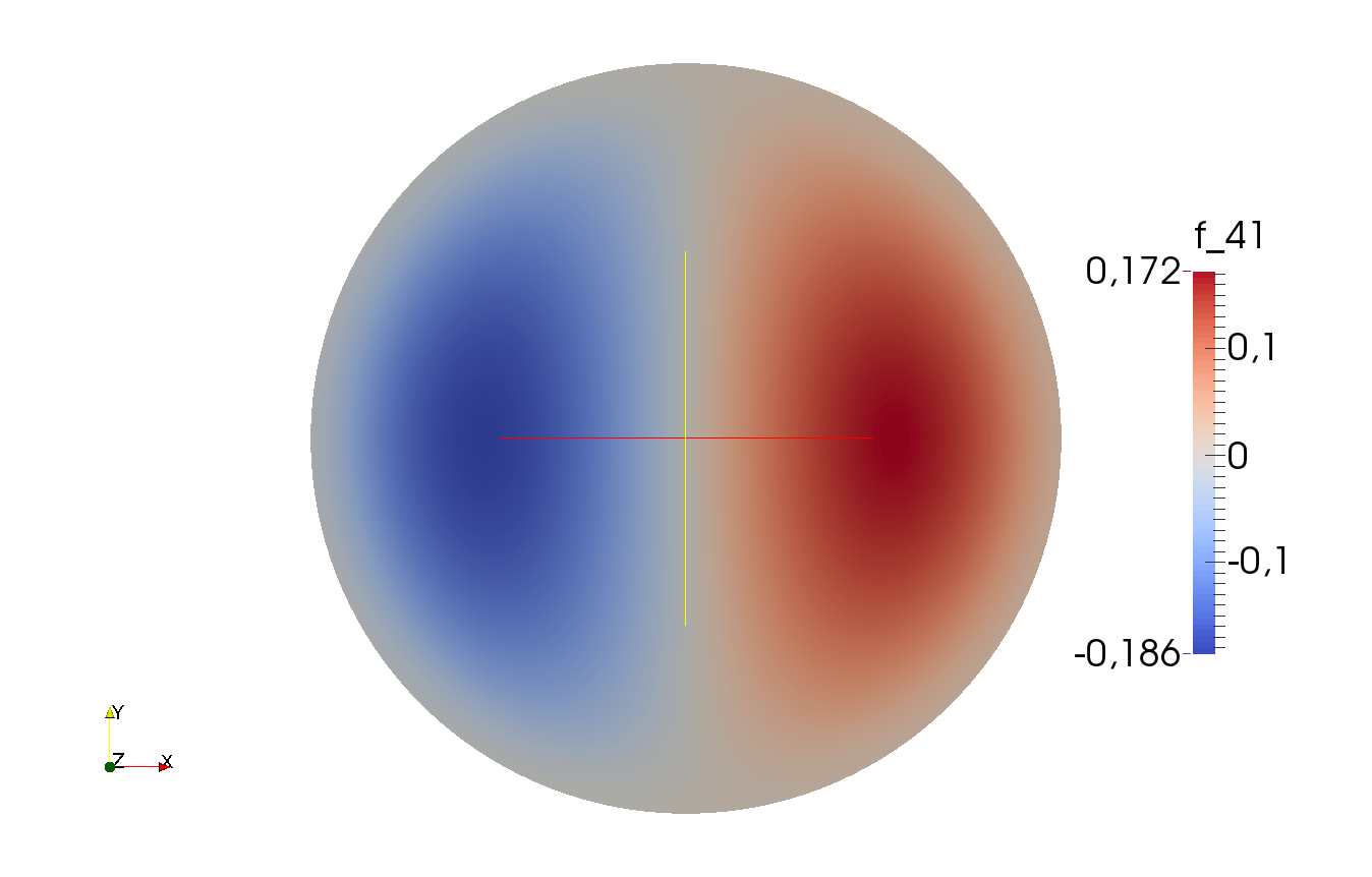
From Theorem 6.8, Corollary 6.9 and Remark 6.10, we expect the error to converge with a rate in and and a rate of in . Furthermore we expect rates of order in . We mention that except the rate in these expectations rely on assumptions we cannot verify rigorously. From Table 1 and the log-log plot of Figure 1 we observe that the numerical results reproduce these rates very accurately, indicating the sharpness of our estimates and the validity of the assumptions. In Figure 2, the solutions and for the Robin boundary problem are presented. From a visual perspective, these solution are almost identical.
 (a) Convergence in -norm.
(b) Convergence in -norm.
(a) Convergence in -norm.
(b) Convergence in -norm.

 (c) Convergence in -norm.
(d) Convergence in -norm.
(c) Convergence in -norm.
(d) Convergence in -norm.
| 0.654779 | 0.755160 | 0.938120 | 0.680350 | |
| 0.199128 (1.71) | 0.337471 (1.16) | 0.381236 (1.30) | 0.444653 (0.61) | |
| 0.049532 (2.01) | 0.126688 (1.41) | 0.117386 (1.70) | 0.242804 (0.87) | |
| 0.011767 (2.07) | 0.044757 (1.50) | 0.032170 (1.87) | 0.124745 (0.96) | |
| 0.002818 (2.06) | 0.015637 (1.52) | 0.008464 (1.93) | 0.062845 (0.99) |
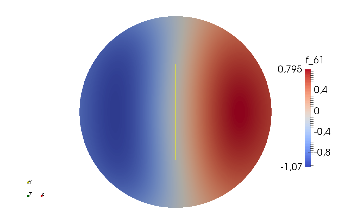
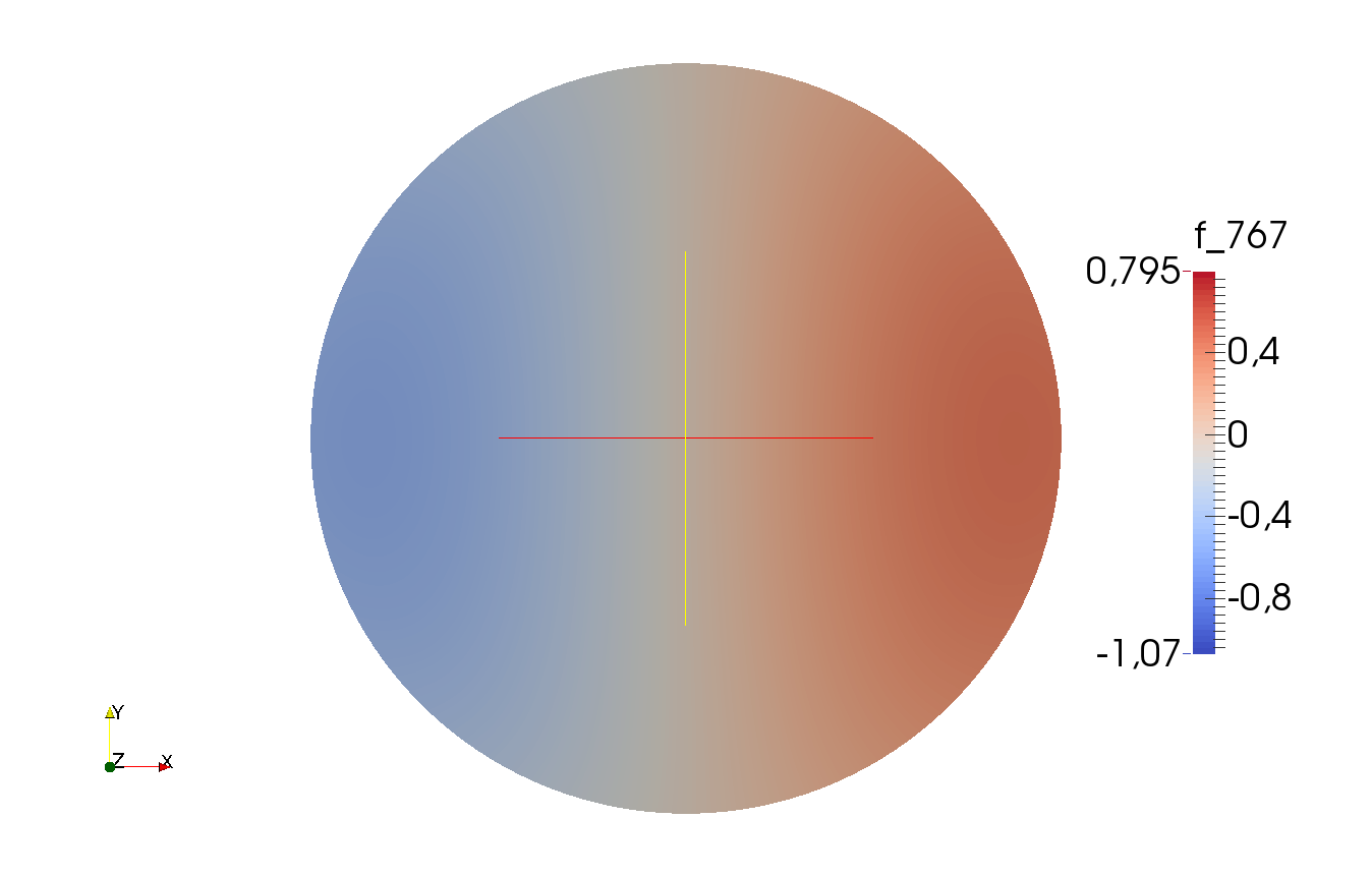 (a) The solution of (30) for .
(b) The solution of
(30) for .
(a) The solution of (30) for .
(b) The solution of
(30) for .
7.2. Case B: Robin BC with discontinuous A matrix
If the parameter A is no longer smooth, but instead , the assumptions for Theorem 6.8 are no longer satisfied. In the second example, we choose a discontinuous as
where are piecewise constant functions with a jump discontinuity close to . All other parameters are the same as in Case A.
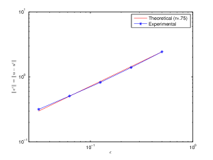
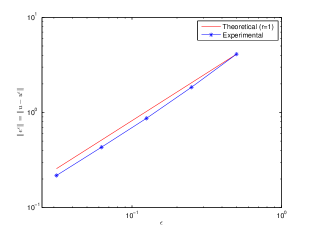
From Table 2 and the log-log plot in Figure 3, we see that the convergence rate of the error is one order worse than in Case A. In particular, we obtain linear convergence in , which is still better than the theoretical result of order we obtain in the non-smooth case for . However we observe clearly the influence of non-smooth on the convergence rate when comparing to case A. For the -convergence, the rate is more inconsistent, as it appears to jump from quadratic to linear when . Although the convergence rate in is only linear in this case, a visual inspection of the solutions shown in Figure 4 reveals that the solution by the diffuse domain method is still almost identical to the exact solution for .
| 0.465577 | 0.622542 | |
| 0.127344 (1.87) | 0.282197 (1.14) | |
| 0.026850 (2.25) | 0.114941 (1.30) | |
| 0.014065 (0.93) | 0.053956 (1.09) | |
| 0.007958 (0.82) | 0.027376 (0.98) |
 (a) The solution of (29).
(b) The solution of
(30).
(a) The solution of (29).
(b) The solution of
(30).
7.3. Case C: Robin BC with non-smooth parameters
Furthermore, in Case C, we also refine the mesh around the discontinuity to increase accuracy.
In Case A, we obtained a convergence rate in of order . Here, everything were smooth. In Case B, when working with a discontinuous matrix A, the convergence rate in drops to order . If, however, the function in (27) is in , but not in for , Theorem 6.5 yields -convergence of, in worst case, order .
To explore this issue numerically, we define
| (46) |
Thus, we get that whenever . All other parameters are given as in Case A. With a similar reasoning as in Lemma 6.3, using and , we expect a rate of convergence of .
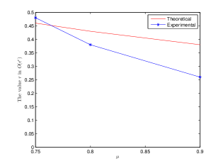
In Figure 5, we see the convergence rate as a function of the parameter in (46). As expected, the convergence rate becomes worse when increases. The experimental rate deteriorates more, however, than the theory suggests. We believe this to be linked to the challenge of the numerical implementation of such a singular function. Although of practical importance, we find that dealing with this particular implementation issue is beyond the scope of this article, and leave it therefore to future research.
7.4. Case D: Dirichlet BC with smooth parameters
We will now study the diffuse domain method for a Dirichlet problem. More particularly, we will compare the solutions and of (34) and (40), respectively. The parameters are given as in case A, with the exception
in order to realize the penalty method. From Theorem 6.13 and Remark 6.15, the choice of should provide a -convergence of order , whereas the choice of should yield a -convergence of order .
 (a) convergence. .
 (b) convergence. .
In Table 3(a), we see the convergence rate of the error when . As expected, the rate is of order in norm. Furthermore, in Table 3(b), we obtain the expected linear convergence in norm. The rates can also be seen in Figure 6.
In Figure 7, we see a solution of (34) and (40), respectively. Although the shape of the solution is visually similar, there is a much larger quantitative difference compared to Case A and B.
| 4.434278 | 2.439132 | |
| 2.301163 (0.95) | 1.394967 (0.81) | |
| 1.365375 (0.75) | 0.823765 (0.76) | |
| 0.878726 (0.64) | 0.509194 (0.69) | |
| 0.566966 (0.63) | 0.318188 (0.68) |
(a) .
| 4.109302 | 2.294747 | |
| 1.844329 (1.16) | 1.188867 (0.95) | |
| 0.868948 (1.09) | 0.616540 (0.95) | |
| 0.432200 (1.01) | 0.331883 (0.89) | |
| 0.217938 (0.99) | 0.186374 (0.83) |
(b) .
 (a) The solution of (34).
(b) The solution of
(40).
(a) The solution of (34).
(b) The solution of
(40).
7.5. Case E: Dirichlet BC with smooth parameters
To guarantee a quadratic convergence in , Theorem 6.8 requires the domain to be . In this final example, we work with the mesh , which is only a Lipschitz domain. All parameters are otherwise identical to in Case A. We see from Figure 8 that the convergence rates are unchanged compared to case A despite the lower regularity of the domain. This gives some hope that our results can be extended to general Lipschitz domain or at least piecewise smooth domains, which remains an open question.
(a) Convergence in -norm.
(b) Convergence in -norm.
 (c) Convergence in -norm.
(d) Convergence in -norm.
(c) Convergence in -norm.
(d) Convergence in -norm.
8. Conclusions
In this work we presented a systematic approach for deriving diffuse domain approaches for second order elliptic problems with usual type of boundary conditions. The advantage of our method is that based on standard variational formulations it readily leads to a relaxed variational formulation, which can be implemented easily, in a straight-forward manner. We presented a self-contained analysis of the error introduced by the diffuse domain method. Depending on the regularity of the data, we could rigorously prove convergence rates. These rates seem to be sharp as shown by numerical experiments. As a by-product of our analysis, we derived trace and embedding theorems as well as Poincaré inequalities for weighted Sobolev spaces which are stable with respect to the relaxation parameter . It remains open to fill a gap to transfer our quadratic convergence results to quadratic convergence results in the -norm which have been proposed in literature. Furthermore, a thorough analysis of numerical methods for the diffuse domain method is left for future work. We are optimistic that time-dependent problems could be treated in a similar manner, further modifications will be needed in the case of evolving surfaces.
Acknowledgements
MB and MS acknowledge support by ERC via Grant EU FP 7 - ERC Consolidator Grant 615216 LifeInverse. MB acknowledges support by the German Science Foundation DFG via EXC 1003 Cells in Motion Cluster of Excellence, Münster, Germany. OLE acknowledges support by DAAD for his one year research stay at WWU Münster.
References
- [1] R. A. Adams. Sobolev spaces. Academic Press [A subsidiary of Harcourt Brace Jovanovich, Publishers], New York-London, 1975. Pure and Applied Mathematics, Vol. 65.
- [2] S. Aland, J. Lowengrub, and A. Voigt. Two-phase flow in complex geometries: a diffuse domain approach. CMES Comput. Model. Eng. Sci., 57(1):77–107, 2010.
- [3] J. M. Arrieta, A. Rodríguez-Bernal, and J. D. Rossi. The best Sobolev trace constant as limit of the usual Sobolev constant for small strips near the boundary. Proc. Roy. Soc. Edinburgh Sect. A, 138(2):223–237, 2008.
- [4] I. Babuška. The finite element method with penalty. Math. Comp., 27:221–228, 1973.
- [5] J. W. Barrett and C. M. Elliott. Fitted and unfitted finite-element methods for elliptic equations with smooth interfaces. IMA J. Numer. Anal., 7(3):283–300, 1987.
- [6] P. Bastian and C. Engwer. An unfitted finite element method using discontinuous Galerkin. Internat. J. Numer. Methods Engrg., 79(12):1557–1576, 2009.
- [7] P. Bochev and R. B. Lehoucq. On the finite element solution of the pure Neumann problem. SIAM Rev., 47(1):50–66, 2005.
- [8] A. Boulkhemair and A. Chakib. On the uniform Poincaré inequality. Comm. Partial Differential Equations, 32(7-9):1439–1447, 2007.
- [9] D. Braess. Finite elements. Cambridge University Press, Cambridge, third edition, 2007. Theory, fast solvers, and applications in elasticity theory, Translated from the German by Larry L. Schumaker.
- [10] F. Brezzi. On the existence, uniqueness and approximation of saddle-point problems arising from Lagrangian multipliers. Rev. Française Automat. Informat. Recherche Opérationnelle Sér. Rouge, 8(R-2):129–151, 1974.
- [11] M. C. Delfour and J.-P. Zolésio. Shapes and geometries, volume 22 of Advances in Design and Control. Society for Industrial and Applied Mathematics (SIAM), Philadelphia, PA, second edition, 2011. Metrics, analysis, differential calculus, and optimization.
- [12] H. Egger and M. Schlottbom. Analysis and regularization of problems in diffuse optical tomography. SIAM J. Math. Anal., 42(5):1934–1948, 2010.
- [13] S. Esedoḡlu, A. Rätz, and M. Röger. Colliding interfaces in old and new diffuse-interface approximations of Willmore-flow. Commun. Math. Sci., 12(1):125–147, 2014.
- [14] S. Franz, R. Gärtner, H.-G. Roos, and A. Voigt. A note on the convergence analysis of a diffuse-domain approach. Comput. Methods Appl. Math., 12(2):153–167, 2012.
- [15] R. Glowinski, T.-W. Pan, and J. Périaux. A fictitious domain method for Dirichlet problem and applications. Comput. Methods Appl. Mech. Engrg., 111(3-4):283–303, 1994.
- [16] J. B. Greer. An improvement of a recent Eulerian method for solving PDEs on general geometries. J. Sci. Comput., 29(3):321–352, 2006.
- [17] P. Grisvard. Elliptic Problems in Nonsmooth Domains. Pitman, Boston, 1985.
- [18] K. Gröger. A -estimate for solutions to mixed boundary value problems for second order elliptic differential equations. Math. Ann., 283(4):679–687, 1989.
- [19] W. Hackbusch and S. A. Sauter. Composite finite elements for the approximation of PDEs on domains with complicated micro-structures. Numer. Math., 75(4):447–472, 1997.
- [20] T. Horiuchi. The imbedding theorems for weighted Sobolev spaces. J. Math. Kyoto Univ., 29(3):365–403, 1989.
- [21] A. Kufner. Weighted Sobolev spaces. A Wiley-Interscience Publication. John Wiley & Sons, Inc., New York, 1985. Translated from the Czech.
- [22] K. Y. Lervag and J. Lowengrub. Analysis of the diffuse-domain method for solving PDEs in complex geometries. arxiv:1407.7480v1, 2014.
- [23] R. J. LeVeque and Z. L. Li. The immersed interface method for elliptic equations with discontinuous coefficients and singular sources. SIAM J. Numer. Anal., 31(4):1019–1044, 1994.
- [24] X. Li, J. Lowengrub, A. Rätz, and A. Voigt. Solving PDEs in complex geometries: a diffuse domain approach. Commun. Math. Sci., 7(1):81–107, 2009.
- [25] F. Liehr, T. Preusser, M. Rumpf, S. Sauter, and L. O. Schwen. Composite finite elements for 3D image based computing. Comput. Vis. Sci., 12(4):171–188, 2009.
- [26] N. G. Meyers. An -estimate for the gradient of solutions of second order elliptic divergence equations. Annali della Scuola Normale Superiore di Pisa - Classe di Scienze, 17(3):189–206, 1963.
- [27] J. Nečas. Direct methods in the theory of elliptic equations. Springer Monographs in Mathematics. Springer, Heidelberg, 2012. Translated from the 1967 French original by Gerard Tronel and Alois Kufner, Editorial coordination and preface by Šárka Nečasová and a contribution by Christian G. Simader.
- [28] B. Opic and A. Kufner. Hardy-type inequalities, volume 219 of Pitman Research Notes in Mathematics Series. Longman Scientific & Technical, Harlow, 1990.
- [29] F. Otto, P. Penzler, A. Rätz, T. Rump, and A. Voigt. A diffuse-interface approximation for step flow in epitaxial growth. Nonlinearity, 17(2):477–491, 2004.
- [30] J. Parvizian, A. Düster, and E. Rank. Finite cell method: - and -extension for embedded domain problems in solid mechanics. Comput. Mech., 41(1):121–133, 2007.
- [31] C. S. Peskin. Numerical analysis of blood flow in the heart. J. Computational Phys., 25(3):220–252, 1977.
- [32] A. Rätz. A new diffuse-interface model for step flow in epitaxial growth. IMA Journal of Applied Mathematics, 2014.
- [33] A. Rätz, A. Voigt, et al. Pde’s on surfaces—a diffuse interface approach. Communications in Mathematical Sciences, 4(3):575–590, 2006.
- [34] M. G. Reuter, J. C. Hill, and R. J. Harrison. Solving PDEs in irregular geometries with multiresolution methods I: Embedded Dirichlet boundary conditions. Comput. Phys. Commun., 183(1):1–7, 2012.
- [35] K. E. Teigen, P. Song, J. Lowengrub, and A. Voigt. A diffuse-interface method for two-phase flows with soluble surfactants. J. Comput. Phys., 230(2):375–393, 2011.
- [36] H. Triebel. Theory of function spaces. III, volume 100 of Monographs in Mathematics. Birkhäuser Verlag, Basel, 2006.