Adaptive observers for nonlinearly parameterized systems subjected to parametric constraints

Abstract

We consider the problem of adaptive observer design in the settings when the system is allowed to be nonlinear in the parameters, and furthermore they are to satisfy additional feasibility constraints. A solution to the problem is proposed that is based on the idea of universal observers and non-uniform small-gain theorem. The procedure is illustrated with an example.

1 Introduction

The problem of adaptive observer design has been in the focus of considerable attention in the past few decades, see e.g. Bastin and Gevers (1988),Marino (1990),Marino and Tomei (1995), Marino and Tomei (1993), Besancon (2000). Available results apply to a broad range of models, including to both linear and non-linear in parameter systems of differential equations Farza et al. (2009),Grip et al. (2011).

Despite this success there is still room for further development. One particular direction is the case when the model parameters are to satisfy additional constraints corresponding to the feasibility regions in the parameter space. Consider for instance the following system Rowat and Selverston (1993)

$$\begin{split}\left(\begin{array}[]{l}\dot{V}\\ \dot{q}\end{array}\right)=&\left(\begin{array}[]{cc}-\tau_{m}^{-1}&-\tau_{m}^{-1}\\ \sigma_{s}\tau_{s}^{-1}&-{\tau}_{s}^{-1}\end{array}\right)\left(\begin{array}[]{l}V\\ q\end{array}\right)\\ &\ \ \ \ \ \ \ \ \ \ \ \ \ \ \ \ +\left(\begin{array}[]{l}1\\ 0\end{array}\right)\frac{A_{f}}{\tau_{m}}\tanh\left(\frac{\sigma_{f}}{A_{f}}V\right),\end{split}$$ (1)

where $\tau_{m}$, $\tau_{s}$, $\sigma_{s}$, $\sigma_{f}$, $A_{f}$ are parameters. Suppose that variable $V$ is available for measurement, and $q$ is not accessible for direct observation. Equations (1) is a modification of the Van-der-Pol equations. Depending on the values of parameters, model (1) is known to exhibit a number of oscillatory solutions with different qualitative dynamics. In systems of this type there may exist a set of solutions for which measured variables, e.g. $V$, look the same, and yet their corresponding parameter values and qualitative underlying dynamics are different. An example of this situation for (1) is illustrated with Fig. 1. Panel $a$ shows numerical approximation of trajectories $V(t)$ in (1) for $\tau_{s}=5$, $\tau_{m}=0.1666$, $A_{f}=1$, $\sigma_{s}=0.9$, and $\sigma_{f}=2$. Upper and lower plots correspond to solutions of (1) passing through $q(0)=0$, $V(0)=1$ and $q(0)=0.179756$, $V(0)=0.199729$, respectively. Panel $b$ contains phase curves of the latter solutions. Panel $c$ presents trajectories $V(t)$ corresponding to the same initial conditions as in panel $a$ but for different parameter values ($\sigma_{s}=1.1$, $\tau_{s}=6.1881$, $\tau_{m}=0.2062$, other parameters remain unchanged). Phase curve of the solution passing through $q(0)=0.179756$, $V(0)=0.199729$ in for these modified parameter values is shown in panel $d$. Grey crosses in panels $b$ and $d$ indicate equilibria.

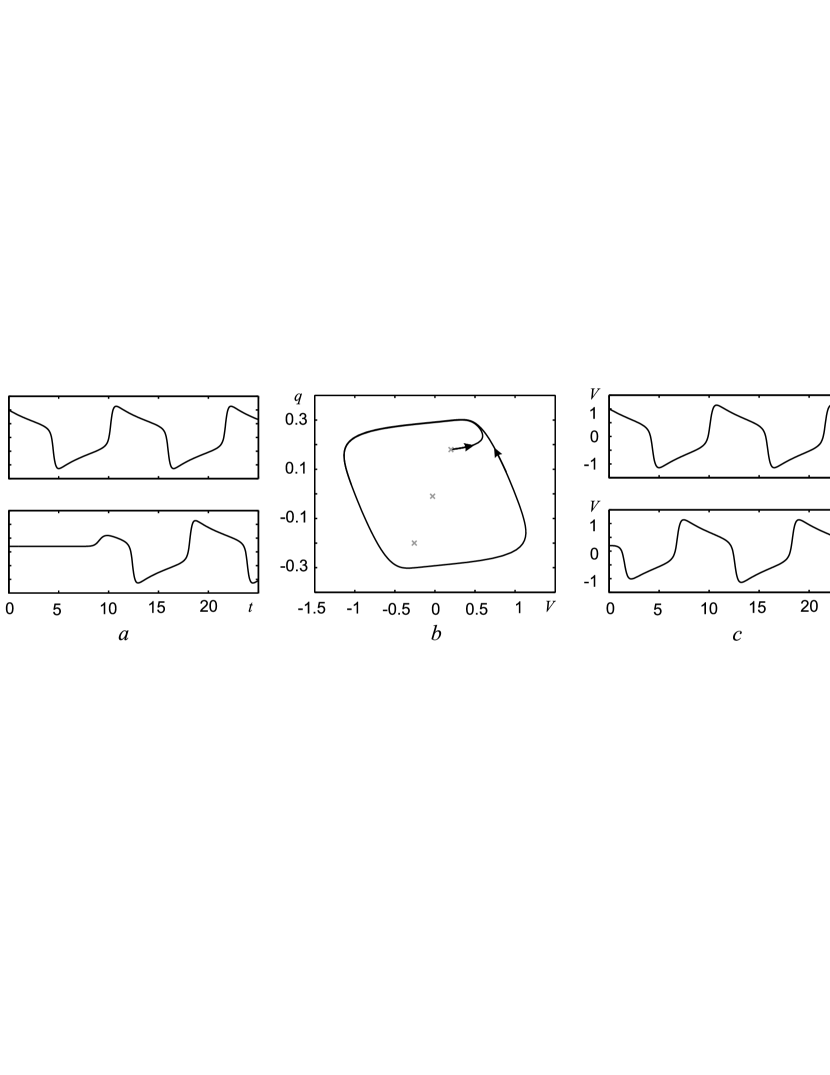
Figure 1: Dynamics of (1) for different parameter values.

Note that trajectories $V(t)$ corresponding to solutions passing through $q(0)=0$, $V(0)=1$ (upper plots in Fig. 1.$a$, Fig. 1.$c$) look nearly identical despite that these trajectories are generated by systems (1) with different parameter values and with different number of equilibria. The overall dynamics of these systems, as the other plots in Fig. 1 suggest, are rather different.

The example above suggests that inferring true parameter values and estimating states from given output observations for systems capable of exhibiting multiple dynamic regimes is not always a well-posed problem. Lack of excitation and/or presence of unmodeled dynamics may result in the values of estimates that are not physically plausible. Hence additional care and precaution must be taken when dealing with such systems. Traditional methods of observer design do not always allow to account for parameter feasibility regions except, possibly, when the set of feasible parameters is convex Grip et al. (2011); Krstic et al. (1995). Thus developing methods enabling to deal with nonlinearly parameterized systems subjected to rather general parametric constraints is needed.

Here we propose an adaptive observer design that satisfies these requirements. Our method is based on the idea of exploiting the advantage of combining search-based optimization with that of direct optimization routines. Observers of this sort were suggested and analyzed in Tyukin et al. (2013). In this work we generalize these results by enabling the observer to account for parameter feasibility regions.

The manuscript is organized as follows. In Section 2 we describe the class of systems considered in the article and provide mathematical statement of the problem. Sections 3 and 4 present main results, Section 5 contains an illustrative example, and Section 6 concludes the paper. Proofs of auxiliary technical statements are provided in the Appendix.

2 Problem Formulation

We will deal with the following class of systems

$$\begin{array}[]{l}\dot{\mathbf{x}}=\mathbf{A}\mathbf{x}+\mbox{\boldmath$\Psi$}(t,{\boldsymbol{\lambda}},y){\boldsymbol{\theta}}+\mathbf{g}(t,{\boldsymbol{\lambda}},y,u)+{\boldsymbol{\xi}}(t),\\ y=\mathbf{C}^{T}\mathbf{x},\ \mathbf{A}=\left(\begin{array}[]{cc}0&\mathbf{I}_{n-1}\\ 0&0\end{array}\right),\ \mathbf{C}=\mathrm{col}(1,0,\dots,0),\end{array}$$ (2)

where $\mbox{\boldmath$\Psi$}:\mathds{R}\times\mathds{R}^{p}\times\mathds{R}\rightarrow\mathds{R}^{n\times m}$, $\mbox{\boldmath$\Psi$},\mathbf{g}\in\mathcal{C}^{1}$, are bounded and Lipschitz in ${\boldsymbol{\lambda}}$, and $\dot{\mbox{\boldmath$\Psi$}}(t,{\boldsymbol{\lambda}},y(t))$, $\dot{\mathbf{g}}(t,{\boldsymbol{\lambda}},y(t),u(t))$ are bounded; ${\boldsymbol{\lambda}}=\mathrm{col}(\lambda_{1},\dots,\lambda_{p})\in\mathds{R}^{p}$, ${\boldsymbol{\theta}}=\mathrm{col}(\theta_{1},\dots,\theta_{m})\in\mathds{R}^{m}$ are unknown parameters, and $u:\mathds{R}\rightarrow\mathds{R}$, $u\in\mathcal{C}^{1}$ is the input. We assume that the values of ${\boldsymbol{\lambda}}$, ${\boldsymbol{\theta}}$ belong to the hypercubes $\Omega_{\lambda}\subset\mathds{R}^{p}$, $\Omega_{\theta}\subset\mathds{R}^{m}$ with known bounds: $\theta_{i}\in[\theta_{i,\min},\theta_{i,\max}]$, $\lambda_{j}\in[\lambda_{j,\min},\lambda_{j,\max}]$. The function ${\boldsymbol{\xi}}\in\mathcal{C}^{0}:\mathds{R}\rightarrow\mathds{R}^{n}$ represents unmodeled dynamics and is supposed to be unknown yet bounded:

$$\|{\boldsymbol{\xi}}(t)\|\leq\Delta_{\xi},\ \Delta_{\xi}\in\mathds{R}_{\geq 0},\ \forall\ t.$$ (3)

Since not all systems (2) may be identifiable, we will require parameter reconstruction only up to a set $\mathcal{E}({\boldsymbol{\lambda}},{\boldsymbol{\theta}})$ of indistinguishable parameters that will be specified later. In addition, we suppose that, for the observed trajectories of (2), true values of parameters ${\boldsymbol{\lambda}},{\boldsymbol{\theta}}$ satisfy the following constraint:

$${\pi}({\boldsymbol{\theta}},{\boldsymbol{\lambda}})=0,$$

where $\pi:\mathds{R}^{m}\times\mathds{R}^{p}\rightarrow\mathds{R}$ is a Lipschitz function. The problem is to determine an auxiliary system, i.e. an adaptive observer: $\dot{\mathbf{q}}=\mathbf{f}(t,y,u,\mathbf{q})$, $\mathbf{f}:\mathds{R}\times\mathds{R}\times\mathds{R}\times\mathds{R}^{q}\rightarrow\mathds{R}^{q}$, $\mathbf{q}(t_{0})=\mathbf{q}_{0}$, $\mathbf{q}\in\mathds{R}^{q}$, and functions $\mathbf{h}_{\theta}:\mathds{R}^{q}\rightarrow\mathds{R}^{m}$, $\mathbf{h}_{\lambda}:\mathds{R}^{q}\rightarrow\mathds{R}^{p}$, $\mathbf{h}_{x}:\mathds{R}^{q}\rightarrow\mathds{R}^{n}$ such that for some given $\mathbf{q}_{0}$, known functions $r_{1},r_{2},r_{3}\in\mathcal{K}$, and all $t_{0}\in\mathds{R}$, the following requirements hold for the observer:

$$\limsup_{t\rightarrow\infty}\|\mathbf{h}_{x}(\mathbf{q}(t,\mathbf{q}_{0}))-\mathbf{x}(t,{\boldsymbol{\lambda}},{\boldsymbol{\theta}},\mathbf{x}_{0})\|\leq r_{1}(\Delta_{\xi})$$ (4)

$$\limsup_{t\rightarrow\infty}\ \mathrm{dist}\left(\left(\begin{array}[]{c}\mathbf{h}_{\lambda}(\mathbf{q}(t,\mathbf{q}_{0}))\\ \mathbf{h}_{\theta}(\mathbf{q}(t,\mathbf{q}_{0}))\end{array}\right),\mathcal{E}({\boldsymbol{\lambda}},{\boldsymbol{\theta}})\right)\leq r_{2}(\Delta_{\xi}),$$ (7)

$$\|\pi(\mathbf{h}_{\theta}(\mathbf{q}(t,\mathbf{q}_{0})),\mathbf{h}_{\lambda}(\mathbf{q}(t,\mathbf{q}_{0})))\|\leq r_{3}(\Delta_{\xi}),$$

where $\Delta_{\xi}$ is defined in (3).

3 Observer Definition

As an observer candidate for (2) we propose the following:

$$\dot{\mathbf{M}}=(\mathbf{A}-\mathbf{B}\mathbf{C}^{T}\mathbf{A})\mathbf{M}+(\mathbf{I}_{n}-\mathbf{B}\mathbf{C}^{T})\mbox{\boldmath$\Psi$}(t,\hat{{\boldsymbol{\lambda}}},y),$$

$$\dot{\hat{{\boldsymbol{\zeta}}}}=\mathbf{A}\hat{{\boldsymbol{\zeta}}}+\boldsymbol{\ell}\,(\mathbf{C}^{T}\hat{{\boldsymbol{\zeta}}}-y)+\mathbf{B}{{\boldsymbol{\varphi}}}^{T}(t,\hat{{\boldsymbol{\lambda}}},y,[\hat{\boldsymbol{\lambda}},y])\hat{{\boldsymbol{\theta}}}$$

$$\ \ \ \ \ \ \ \ \ \ \ \ \ \ +\mathbf{g}(t,\hat{{\boldsymbol{\lambda}}},y,u),$$ (8)

$$\dot{\hat{{\boldsymbol{\theta}}}}=-\gamma_{\theta}(\mathbf{C}^{T}\hat{{\boldsymbol{\zeta}}}-y){{\boldsymbol{\varphi}}}(t,\hat{{\boldsymbol{\lambda}}},y,[\hat{\boldsymbol{\lambda}},y]),\ \gamma_{\theta}\in\mathds{R}_{>0},$$

$$\hat{\mathbf{x}}=\hat{{\boldsymbol{\zeta}}}+\mathbf{M}\hat{{\boldsymbol{\theta}}},$$

where $\mathbf{B}=\mathrm{col}\left(1,b_{1},\dots,b_{n-1}\right)$ is a vector such that the polynomial $s^{n-1}+b_{1}s^{n-2}+\dots+b_{n-1}$ is Hurwitz, $\mathbf{M}(t_{0})=0$,

$${{\boldsymbol{\varphi}}}^{T}(t,\hat{{\boldsymbol{\lambda}}},y,[\hat{\boldsymbol{\lambda}},y])=\mathbf{C}^{T}\mathbf{A}\mathbf{M}(t,[\hat{{\boldsymbol{\lambda}}},y])+\mathbf{C}^{T}\mbox{\boldmath$\Psi$}(t,\hat{{\boldsymbol{\lambda}}},y),$$

and $\hat{\boldsymbol{\lambda}}$ is defined as

$$\begin{split}&\left\{\begin{array}[]{ll}\dot{{s}}_{2j-1}&=\gamma\sigma(\|y-\hat{y}\|_{\varepsilon}+\|\pi(\hat{{\boldsymbol{\theta}}},\hat{{\boldsymbol{\lambda}}})\|_{\varepsilon})\cdot\omega_{j}\cdot({s}_{2j-1}\\ &-{s}_{2j}-{s}_{2j-1}({s}_{2j-1}^{2}+{s}_{2j}^{2}))\\ \dot{{s}}_{2j}&=\gamma\sigma(\|y-\hat{y}\|_{\varepsilon}+\|\pi(\hat{{\boldsymbol{\theta}}},\hat{{\boldsymbol{\lambda}}})\|_{\varepsilon})\cdot\omega_{j}\cdot({s}_{2j-1}\\ &+{s}_{2j}-{s}_{2j}({s}_{2j-1}^{2}+{s}_{2j}^{2}))\\ \hat{\lambda}_{j}&=\beta_{j}(\mathbf{s}),\ j=\{1,\dots,p\},\end{array}\right.\\ \beta_{j}(\mathbf{s})&=\lambda_{j,\min}+\frac{\lambda_{j,\max}-\lambda_{j,\min}}{2}({s}_{2j-1}+1)\end{split}$$ (9)

$$\mathbf{s}_{0}=\mathbf{s}(t_{0}):\ {s}_{2j-1}^{2}(t_{0})+{s}_{2j}^{2}(t_{0})=1,$$ (10)

where $\gamma\in\mathds{R}_{>0}$, $\sigma:\mathds{R}_{\geq 0}\rightarrow\mathds{R}_{\geq 0}$ is a bounded Lipschitz function:

$$\begin{split}\exists\ D_{\sigma},\ M_{\sigma}\in\mathds{R}_{>0}:&\\ \sigma(\upsilon)\leq M_{\sigma},&\ \sigma(\upsilon)\leq D_{\sigma}\upsilon\ \ \forall\ \upsilon\geq 0\end{split}$$

such that $\sigma(\upsilon)>0$ for $\upsilon>0$, and $\sigma(0)=0$. Parameters $\omega_{j}\in\mathds{R}_{>0}$ in (9) are supposed to be rationally-independent:

$$\sum_{j=1}^{p}\omega_{j}k_{j}\neq 0,\ \forall\ k_{j}\in\mathds{Z}.$$ (11)

4 Main Result

As it is often the case in the domain of adaptive observer design, state and parameter reconstruction of the observer is subjected to some form of persistency of excitation (PE). Insufficient excitation have detrimental effect on the quality and robustness of estimation (see examples in Fig. 1). Here we employ the following modifications of the PE conditions:

Definition 1 (Loria and Panteley (2003))

A function $\boldsymbol{\alpha}:\mathds{R}_{\geq t_{0}}\times\Omega_{\lambda}\rightarrow\mathds{R}^{p}$ is said to be $\lambda$-Uniformly Persistently Exciting ($\lambda$-UPE with $T$, $\mu$), denoted by $\boldsymbol{\alpha}(t,{\boldsymbol{\lambda}})\in\lambda{\rm UPE}(T,\mu)$, if there exist $T,\mu\in\mathds{R}_{>0}$:

$$\int_{t}^{t+T}\boldsymbol{\alpha}(\tau,{\boldsymbol{\lambda}})\boldsymbol{\alpha}^{T}(\tau,{\boldsymbol{\lambda}}){\rm d}\tau\geq\mu\mathbf{I},\ \forall\ t\geq t_{0},\ {\boldsymbol{\lambda}}\in\Omega_{\lambda}.$$ (12)

Uniform persistency of excitation requires existence of $\mu\in\mathds{R}_{>0}$ in (12) that is independent on ${\boldsymbol{\lambda}}$ for all ${\boldsymbol{\lambda}}\in\Omega_{\lambda}$.

Definition 2

Let $\mathcal{E}$ be a set-valued map defined on $\mathcal{D}\subset\mathds{R}^{d}$ and associating a subset of $\mathcal{D}$ to every $\mathbf{p}\in\mathcal{D}$. A function $\boldsymbol{\alpha}:\mathds{R}\times\mathcal{D}\times\mathcal{D}\rightarrow\mathds{R}^{k}$ is said to be weakly Nonlinearly Persistently Exciting in $\mathbf{p}$ wrt $\mathcal{E}$ (wNPE with $L,\beta,\mathcal{E}$ ), denoted by $\boldsymbol{\alpha}(t,\mathbf{p},\mathbf{p}^{\prime})\in{\rm wNPE}(L,\beta,\mathcal{E})$, if there exist $L\in\mathds{R}_{>0}$, $t_{1}\geq t_{0}$, and $\beta\in\mathcal{K}_{\infty}$:

$$\begin{split}&\forall\ t\geq t_{1},\ \mathbf{p},\mathbf{p}^{\prime}\in\mathcal{D}\ \exists\ t^{\prime}\in[t,t+L]:\\ &\ \ \ \ \ \ \ \ \|\boldsymbol{\alpha}(t^{\prime},\mathbf{p},\mathbf{p}^{\prime})\|\geq\beta\left({\rm dist}(\mathcal{E}(\mathbf{p}),\mathbf{p}^{\prime})\right).\end{split}$$ (13)

Finally, consider

$$\begin{split}&\boldsymbol{\eta}(t,{\boldsymbol{\lambda}},{\boldsymbol{\theta}},{\boldsymbol{\lambda}}^{\prime},{\boldsymbol{\theta}}^{\prime})={\boldsymbol{\varphi}}^{T}(t,{\boldsymbol{\lambda}}^{\prime},y(t),[{\boldsymbol{\lambda}}^{\prime},y])({\boldsymbol{\theta}}^{\prime}-{\boldsymbol{\theta}})+\\ &\mathbf{C}^{T}(\mbox{\boldmath$\Psi$}(t,{\boldsymbol{\lambda}}^{\prime},y(t))-\mbox{\boldmath$\Psi$}(t,{\boldsymbol{\lambda}},y(t)){\boldsymbol{\theta}}+g_{1}(t,{\boldsymbol{\lambda}}^{\prime},y(t),u(t))-\\ &g_{1}(t,{\boldsymbol{\lambda}},y(t),u(t))+q(t,{\boldsymbol{\lambda}}^{\prime},{\boldsymbol{\lambda}},{\boldsymbol{\theta}}),\end{split}$$

$q(t,{\boldsymbol{\lambda}}^{\prime},{\boldsymbol{\lambda}},{\boldsymbol{\theta}})=\tilde{\mathbf{C}}\mathbf{z}$, $\dot{\mathbf{z}}=\Lambda\mathbf{z}+\mathbf{G}((\Psi(t,{\boldsymbol{\lambda}}^{\prime},y(t))-\Psi(t,{\boldsymbol{\lambda}},y(t))){\boldsymbol{\theta}}+\mathbf{g}(t,{\boldsymbol{\lambda}}^{\prime},y(t),u(t))-\mathbf{g}(t,{\boldsymbol{\lambda}},y(t),u(t)))$, $\mathbf{z}(t_{0})=0$, and $\tilde{\mathbf{C}}$, $\Lambda$, $\mathbf{G}$ are defined as

$$\begin{split}&\tilde{\mathbf{C}}=\mathrm{col}(1,0,\dots,0),\tilde{\mathbf{C}}\in\mathds{R}^{n-1},\ \Lambda=\left(\begin{array}[]{ccc}-\mathbf{b}&\begin{array}[]{c}\vdots\\ \vdots\end{array}&\begin{array}[]{c}I_{n-2}\\ 0\end{array}\end{array}\right),\\ &\mathbf{G}=\left(\begin{array}[]{cc}-{\mathbf{b}}&I_{n-1}\end{array}\right),\ \mathbf{b}=(b_{1},\dots,b_{n-1})^{T}.\end{split}$$

The following can now be stated:

Theorem 3

Consider (2), (3), (9)–(11). Suppose that the restriction of the function ${\boldsymbol{\varphi}}(t,{\boldsymbol{\lambda}},y(t),[{\boldsymbol{\lambda}},y])$ in (3) on $\mathds{R}\times\Omega_{\lambda}$ is $\lambda$-uniformly persistently exiting, and the function $\boldsymbol{\alpha}(t,({\boldsymbol{\lambda}},{\boldsymbol{\theta}}),({\boldsymbol{\lambda}}^{\prime},{\boldsymbol{\theta}}^{\prime}))=\boldsymbol{\eta}(t,{\boldsymbol{\lambda}},{\boldsymbol{\theta}},{\boldsymbol{\lambda}}^{\prime},{\boldsymbol{\theta}}^{\prime})$ is weakly nonlinearly persistently exciting in $({\boldsymbol{\lambda}},{\boldsymbol{\theta}})$ wrt to the map $\mathcal{E}$:

$$\begin{split}&\mathcal{E}({\boldsymbol{\lambda}},{\boldsymbol{\theta}})=\{({\boldsymbol{\lambda}}^{\prime},{\boldsymbol{\theta}}^{\prime}),\ {\boldsymbol{\lambda}}^{\prime}\in\mathds{R}^{p},\ {\boldsymbol{\theta}}^{\prime}\in\mathds{R}^{m}|\mathbf{B}({\boldsymbol{\theta}}^{\prime}-{\boldsymbol{\theta}})^{T}\cdot\\ &{\boldsymbol{\varphi}}(t,{\boldsymbol{\lambda}}^{\prime},y(t),[{\boldsymbol{\lambda}}^{\prime},y])+(\mbox{\boldmath$\Psi$}(t,{\boldsymbol{\lambda}}^{\prime},y(t))-\mbox{\boldmath$\Psi$}(t,{\boldsymbol{\lambda}},y(t))){\boldsymbol{\theta}}\\ &+\mathbf{g}(t,{\boldsymbol{\lambda}}^{\prime},y(t),u(t))-\mathbf{g}(t,{\boldsymbol{\lambda}},y(t),u(t))=0,\ \forall\ t\geq t_{0}\}.\end{split}$$

Then there exist a constant $\bar{\gamma}\in\mathds{R}_{>0}$ and functions $r_{1},r_{2},r_{3},r_{4}\in\mathcal{K}$ such that if $\gamma,\varepsilon$ are the corresponding parameters of (9), and $\gamma\in(0,\bar{\gamma})$, $\varepsilon>r_{1}(\Delta_{\xi})$, then

$$\limsup_{t\rightarrow\infty}\mathrm{dist}\left(\left(\begin{array}[]{c}\hat{\boldsymbol{\lambda}}(t)\\ \hat{\boldsymbol{\theta}}(t)\end{array}\right),\mathcal{E}({\boldsymbol{\lambda}},{\boldsymbol{\theta}})\right)\leq r_{2}(\varepsilon).$$ (16)

$$\limsup_{t\rightarrow\infty}\|\hat{\mathbf{x}}(t)-\mathbf{x}(t)\|\leq r_{3}(\varepsilon),$$ (17)

$$\limsup_{t\rightarrow\infty}\|\pi(\hat{{\boldsymbol{\theta}}}(t),\hat{{\boldsymbol{\lambda}}}(t))\|\leq r_{4}(\varepsilon).$$ (18)

Proof of Theorem 3. The idea behind the proof of the theorem is similar to that of presented in Tyukin et al. (2013) and, taking space limitations into account, we present just a sketch here. Note that the first row of $\mathbf{M}$ in the observer system is zero for all $t\geq t_{0}$, and that $\hat{y}=\mathbf{C}^{T}\hat{\mathbf{x}}=\mathbf{C}^{T}\hat{{\boldsymbol{\zeta}}}$. Moreover, since $\mbox{\boldmath$\Psi$}(t,\hat{{\boldsymbol{\lambda}}},y)$ is bounded and Lipschitz in $\hat{{\boldsymbol{\lambda}}}$, the variables $\mathbf{M}(t,[\hat{{\boldsymbol{\lambda}}},y]),\dot{\mathbf{M}}(t,[\hat{{\boldsymbol{\lambda}}},y])$ are also bounded, and ${\mathbf{M}}(t,[\hat{\boldsymbol{\lambda}},y])$ is Lipschitz in $\hat{{\boldsymbol{\lambda}}}$ for $\hat{\boldsymbol{\lambda}}=\mathrm{const}$. Let ${\boldsymbol{\zeta}}=\mathbf{x}-\mathbf{M}{\boldsymbol{\theta}}$, then

$$\begin{split}{\dot{\boldsymbol{\zeta}}}=&\mathbf{A}{\boldsymbol{\zeta}}+\mathbf{B}{\boldsymbol{\varphi}}(t,\hat{\boldsymbol{\lambda}},y,[\hat{{\boldsymbol{\lambda}}},y]){\boldsymbol{\theta}}+(\mbox{\boldmath$\Psi$}(t,{\boldsymbol{\lambda}},y,u)\\ &-\mbox{\boldmath$\Psi$}(t,\hat{\boldsymbol{\lambda}},y,u)){\boldsymbol{\theta}}+\mathbf{g}(t,{\boldsymbol{\lambda}},y,u)+{\boldsymbol{\xi}}(t).\end{split}$$

Dynamics of (2), (3) in the coordinates $\mathbf{e}_{1}=\hat{{\boldsymbol{\zeta}}}-\mathbf{x}+\mathbf{M}{\boldsymbol{\theta}}$, $\mathbf{e}_{2}=\hat{{\boldsymbol{\theta}}}-{\boldsymbol{\theta}}$ is

$$\begin{pmatrix}\dot{\mathbf{e}}_{1}\\ \dot{\mathbf{e}}_{2}\end{pmatrix}=\begin{pmatrix}\mathbf{A}+\boldsymbol{\ell}\,\mathbf{C}^{T}&\mathbf{B}{\boldsymbol{\varphi}}^{T}(t,\hat{\boldsymbol{\lambda}},y,[\hat{\boldsymbol{\lambda}},y])\\ -\gamma_{\theta}{\boldsymbol{\varphi}}(t,\hat{\boldsymbol{\lambda}},y,[\hat{\boldsymbol{\lambda}},y])\mathbf{C}^{T}&0\end{pmatrix}$$

$$\ \ \ \ \ \ \ \ \ \ \ \ \ \ \ \times\begin{pmatrix}\mathbf{e}_{1}\\ \mathbf{e}_{2}\end{pmatrix}+\begin{pmatrix}\tilde{\mathbf{v}}(t,\hat{\boldsymbol{\lambda}},{\boldsymbol{\lambda}},y,u)\\ 0\end{pmatrix}$$ (19)

where

$$\begin{split}\tilde{\mathbf{v}}(t,\hat{\boldsymbol{\lambda}},{\boldsymbol{\lambda}},y,u)&=(\mbox{\boldmath$\Psi$}(t,\hat{\boldsymbol{\lambda}},y)-\mbox{\boldmath$\Psi$}(t,{{\boldsymbol{\lambda}}},y)){\boldsymbol{\theta}}\\ &+\mathbf{g}(t,\hat{\boldsymbol{\lambda}},y,u)-\mathbf{g}(t,{\boldsymbol{\lambda}},y,u)-{\boldsymbol{\xi}}(t).\end{split}$$

Since the pair $\mathbf{A}$, $\mathbf{C}$ is observable one can always find an $\boldsymbol{\ell}\,$ so that dynamics of the homogeneous part of (4) is exponentially stable subject to persistency of excitation of ${\boldsymbol{\varphi}}(t,\hat{\boldsymbol{\lambda}},y,[\hat{\boldsymbol{\lambda}},y])$. The latter condition is ensured by picking the values of $\gamma$ sufficiently small (see Tyukin et al. (2013)).

Recall that the function $\pi$ is Lipschitz and that $\pi({\boldsymbol{\theta}},{\boldsymbol{\lambda}})=0$. Therefore

$$\begin{split}\|\pi(\hat{{\boldsymbol{\theta}}},\hat{{\boldsymbol{\lambda}}})\|&=\|\pi(\hat{\boldsymbol{\theta}},\hat{\boldsymbol{\lambda}})-\pi({\boldsymbol{\theta}},{\boldsymbol{\lambda}})\|\leq L_{1}\|\hat{\boldsymbol{\theta}}-{\hat{\boldsymbol{\theta}}}\|\\ &+L_{2}\|\hat{\boldsymbol{\lambda}}-{\boldsymbol{\lambda}}\|.\end{split}$$ (20)

Furthermore, notice that

1. $|a|\leq|b|\Rightarrow\|a\|_{\varepsilon}\leq\|b\|_{\varepsilon}$

2. $\||a|+|b|\|_{\varepsilon}\leq\|a\|_{\varepsilon}+|b|\ \forall\ a,b\in\mathds{R}$

3. $\|La\|_{\varepsilon}=|L|\|a\|_{\frac{\varepsilon}{|L|}},\ a\in\mathds{R}$

4. $\|a\|_{\varepsilon}+\|b\|_{\varepsilon}\leq 2\|a,b\|_{\varepsilon}$, where $\|a,b\|_{\varepsilon}=\sqrt{\|a\|_{\varepsilon}^{2}+\|b\|_{\varepsilon}^{2}}$.

Hence, using (20) and applying properties 1–4 above to $\|\pi(\hat{\boldsymbol{\theta}},\hat{\boldsymbol{\lambda}})\|_{\varepsilon}$ we obtain:

$$\begin{split}\|\pi(\hat{{\boldsymbol{\theta}}},\hat{{\boldsymbol{\lambda}}})\|_{\varepsilon}&\leq\|L_{1}\|\hat{\boldsymbol{\theta}}-{\boldsymbol{\theta}}\|\|_{\varepsilon}+L_{2}\|\hat{\boldsymbol{\lambda}}-{\boldsymbol{\lambda}}\|=L_{1}\|\hat{\boldsymbol{\theta}}-{\boldsymbol{\theta}}\|_{\frac{\varepsilon}{L_{1}}}\\ &+L_{2}\|\hat{\boldsymbol{\lambda}}-{\boldsymbol{\lambda}}\|.\end{split}$$

Therefore, since $\|\mathbf{C}\|=1$, $\|\mathbf{C}^{T}(\mathbf{x}-\hat{\mathbf{x}})\|_{\varepsilon}+\|\pi(\hat{\boldsymbol{\theta}},\hat{\boldsymbol{\lambda}})\|_{\varepsilon}\leq\|\hat{\mathbf{x}}-\mathbf{x}\|_{\varepsilon}+L_{1}\|\hat{\boldsymbol{\theta}}-{\boldsymbol{\theta}}\|_{\frac{\varepsilon}{L_{1}}}+L_{2}\|\hat{\boldsymbol{\lambda}}-{\boldsymbol{\lambda}}\|$. Denoting $\epsilon=\frac{\varepsilon}{L_{1}}$ results in

$$\begin{split}&\|\mathbf{C}^{T}(\mathbf{x}-\hat{\mathbf{x}})\|_{\varepsilon}+\|\pi(\hat{\boldsymbol{\theta}},\hat{\boldsymbol{\lambda}})\|_{\varepsilon}\leq\|\hat{\mathbf{x}}-\mathbf{x}\|_{\epsilon}\\ &+L_{1}\|\hat{\boldsymbol{\theta}}-{\boldsymbol{\theta}}\|_{\epsilon}+L_{2}\|\hat{\boldsymbol{\lambda}}-{\boldsymbol{\lambda}}\|.\end{split}$$ (21)

Finally, taking (21) into account, and repeating the argument provided in Tyukin et al. (2013) in which Lemma 8 is replaced with Lemma 4 below (see Appendix for the proof) one can complete the proof of the theorem.

Lemma 4

Consider a system governed by the following set of equations

$$\|\mathbf{x}(t)\|\leq\beta(t-t_{0})\|\mathbf{x}(t_{0})\|+c\|h(\tau)\|_{\infty,[t_{0},t]}+\Delta,$$ (22)

$$-\int_{t_{0}}^{t}\gamma_{0}(\|\mathbf{x}(\tau)+\mathbf{d}(\tau)\|_{\varepsilon}+M|h(\tau)|)d\tau$$

$$\ \ \ \ \ \ \ \ \ \ \ \ \ \ \ \ \ \ \ \ \ \ \ \ \ \ \ \ \ \ \leq h(t)-h(t_{0})\leq 0,\ \forall\ t\geq t_{0},$$

where $\mathbf{x}:\mathds{R}\rightarrow\mathds{R}^{n}$, $h:\mathds{R}\rightarrow\mathds{R}$ are trajectories reflecting the evolution of the system’s state, $\mathbf{d}:\mathds{R}\rightarrow\mathds{R}^{n}$, $\|\mathbf{d}(\tau)\|_{\infty,[t_{0},\infty)}\leq\Delta_{d}$ is a continuous and bounded function on $[t_{0},\infty)$, $\beta(\cdot)$ is a strictly monotonically decreasing function with, $\beta(0)\geq 1$, $\lim_{s\rightarrow\infty}\beta(s)=0$; $c,\Delta\in\mathds{R}_{>0}$, and $\gamma_{0}:\mathds{R}\rightarrow\mathds{R}_{\geq 0}$:

$$|\gamma_{0}(s)|\leq D_{\gamma}|s|.$$ (23)

Then trajectories $\mathbf{x}(t)$, $h(t)$ in (22) are bounded in forward time, for $t\geq t_{0}$, provided that the following conditions hold for some $d\in(0,1)$, $\kappa\in(1,\infty)$:

$$\varepsilon \geq \Delta\left(1+\beta(0)\frac{\kappa}{\kappa-d}\right)+\Delta_{d},$$ (24)

$$D_{\gamma} \leq \frac{\kappa-1}{\kappa}\left[\beta^{-1}\left(\frac{d}{\kappa}\right)\right]^{-1}\times$$

$$\times\frac{h(t_{0})}{\beta(0)\|\mathbf{x}(t_{0})\|+|h(t_{0})|(c(1+\kappa\beta(0)/(1-d))+M)}.$$

$\square$

5 Example

Consider system (1). Let us first transform (1) into (2). Applying the following coordinate transformation $\left(\begin{array}[]{c}V^{\prime}\\ q^{\prime}\end{array}\right)=\left(\begin{array}[]{cc}1&0\\ 0&-\tau_{m}^{-1}\\ \end{array}\right)\left(\begin{array}[]{c}V\\ q\end{array}\right)$ we get:

$$\frac{dV^{\prime}}{dt} =-\tau_{m}^{-1}{V^{\prime}}+\tau_{m}^{-1}{A_{f}\tanh[(\sigma_{f}/A_{f})V^{\prime}]}+q^{\prime},$$

$$\frac{dq^{\prime}}{dt} =-{\tau_{s}}^{-1}{q^{\prime}}-{(\tau_{s}\tau_{m})}^{-1}{\sigma_{s}}V^{\prime},$$

and using an additional change of coordinates $\left(\begin{array}[]{c}x_{1}\\ x_{2}\end{array}\right)=\left(\begin{array}[]{cc}1&0\\ \tau_{s}^{-1}&1\\ \end{array}\right)\left(\begin{array}[]{c}V^{\prime}\\ q^{\prime}\end{array}\right)$ we arrive at:

$$\dot{x}_{1}= x_{2}-\left({\tau_{m}^{-1}}+{\tau_{s}^{-1}}\right)x_{1}+\tau_{m}^{-1}A_{f}\tanh[(\sigma_{f}/A_{f})x_{1}],$$

$$\dot{x}_{2}= -(\tau_{s}\tau_{m})^{-1}\left(1+{\sigma_{s}}\right)x_{1}$$

$$+{(\tau_{s}\tau_{m})^{-1}}A_{f}\tanh[(\sigma_{f}/A_{f})x_{1}].$$

Noticing that $y=C^{T}\mathbf{x}=x_{1}$ and denoting $\theta_{1}=-\frac{1}{\tau_{m}}-\frac{1}{\tau_{s}},\quad\theta_{2}=\frac{1}{\tau_{m}}A_{f},\quad\theta_{3}=\frac{-1-\sigma_{s}}{\tau_{s}\tau_{m}},\quad\theta_{4}=\frac{1}{\tau_{s}\tau_{m}}A_{f},\quad\lambda=\frac{\sigma_{f}}{A_{f}}$, we obtain

$$\dot{x_{1}} =x_{2}+\theta_{1}y+\theta_{2}\tanh[\lambda y],$$

$$\dot{x_{2}} =\theta_{3}y+\theta_{4}\tanh[\lambda y],$$

$$y =x_{1}.$$

The above equations in the form (2) where

$$\mathbf{A}=\left(\begin{array}[]{cc}0&1\\ 0&0\\ \end{array}\right),\quad\mathbf{\Psi}=\left(\begin{array}[]{cccc}y&\tanh[\lambda y]&0&0\\ 0&0&y&\tanh[\lambda y]\\ \end{array}\right),$$

$${\boldsymbol{\theta}}=(\theta_{1},\theta_{2},\theta_{3},\theta_{4}),\ \mathbf{g}=\left(\begin{array}[]{c}0\\ 0\\ \end{array}\right),\quad\mathbf{C}^{T}=\left(\begin{array}[]{cc}1&0\\ \end{array}\right).$$

Parameters of the observer (3), (9) were set as follows:

$$\mathbf{B}=\left(\begin{array}[]{c}1\\ 1\\ \end{array}\right),\quad\mathbf{l}=\left(\begin{array}[]{c}-2\\ -1\\ \end{array}\right),\quad\gamma_{\mathbf{\theta}}=4,\ \gamma=0.002.$$

It is clear that original state parameter values of (1) can be recovered from $\mathbf{x}$, ${\boldsymbol{\theta}}$, and $\lambda$ in accordance with the inverse transform:

$$\tau_{s}={\theta_{2}}/{\theta_{4}},\quad\tau_{m}=-1/({\theta_{1}+{1}/{\tau_{s}}}),\quad A_{f}=\theta_{2}\tau_{m},$$

$$\sigma_{s}=-\theta_{3}\tau_{s}\tau_{m}-1,\ \sigma_{f}=\lambda A_{f},\ \mathbf{x}=\mathbf{{\boldsymbol{\zeta}}}+\mathbf{M}\mathbf{{\boldsymbol{\theta}}};$$

$$\left(\begin{array}[]{c}V\\ q\\ \end{array}\right)=\left(\begin{array}[]{cc}1&0\\ {\tau_{s}}{\tau_{m}^{-1}}&-{\tau_{m}^{-1}}\\ \end{array}\right)\left(\begin{array}[]{c}x_{1}\\ x_{2}\\ \end{array}\right).$$

True parameter value and initial conditions were set to:

$$\tau_{s}=5,\quad\tau_{m}=0.1666,\quad A_{f}=1,\quad\sigma_{s}=0.8,\quad\sigma_{f}=2;$$

$$\mathbf{\theta}=(-6.2,6,-2.16,1.2),\ \lambda=2,\ \left(\begin{array}[]{c}V_{0}\\ q_{0}\\ \end{array}\right)=\left(\begin{array}[]{c}1\\ 0\\ \end{array}\right).$$

Depending on specific parameter values, the model may have $1$ or $3$ distinct equilibria in the system state space. One of these equilibria is always at the origin, $(0;0)$, and the other two are located in the first and third quadrant, respectively. The corresponding bifurcation diagram derived at $A_{f}=1$, $\sigma_{f}=2$ and $\sigma_{s}\in[0.8,1.2]$ is shown in Fig. 2. Blue, green and red curves show the values of the $V$-coordinate, $V_{e}$, of the equilibria for various values of $\sigma_{s}$. White circles correspond to solutions shown in panels $b$, $d$ in Fig. 1.

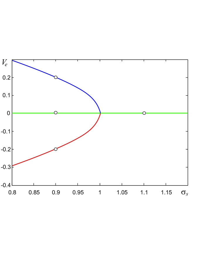
Figure 2: Bifurcation diagram of system (1).

If $\sigma_{s}\leq\sigma_{f}-1$ the non-zero equilibria disappear. In our particular case the system has the following three equilibria: $(0;0)$, $(0.292;0.2336)$, $(-0.292;-0.2336)$. The first equilibrium is a saddle point (one positive and one negative real eigenvalues), and the other two are unstable nodes (both eigenvalues are real and positive).

We supposed that information about qualitative dynamics of the original system has been made available in the form of the number of equilibria and their qualitative characterizations (saddle point, stable/unstable nodes). In particular, we assumed that the following is known:

• The total number of distinct equilibria in the system is $3$;

• Eigenvalues corresponding to zero equilibrium position are real (discriminant $>0$);

• Signs of the eigenvalues at zero equilibrium are different.

The first restriction is satisfied if

$$\sigma_{s}>\sigma_{f}-1.$$ (26)

Consider the other two remaining conditions. Characteristic polynomial of the Jacobian of the right-hand side of (1) is: $s^{2}+\left((1-\sigma_{f}){\tau_{m}^{-1}}+{\tau_{s}^{-1}}\right)s+({1-\sigma_{f}+\sigma_{s}})(\tau_{s}\tau_{m})^{-1}$. The second condition is therefore equivalent to that the discriminant $D$ of this quadratic is positive:

$$D=\left(\frac{1-\sigma_{f}}{\tau_{m}}+\frac{1}{\tau_{s}}\right)^{2}-4\left(\frac{1-\sigma_{f}+\sigma_{s}}{\tau_{s}\tau_{m}}\right)>0.$$ (27)

The third and the final condition can now be expressed as:

$$\left|\frac{1-\sigma_{f}}{\tau_{m}}+\frac{1}{\tau_{s}}\right|<\sqrt{D}.$$ (28)

Parametric constraints (26)–(28) are in the form of strict inequalities. The proposed observer design, however, requires that parametric constraints are formulated in the form of equalities. For this purpose we introduce:

$$\begin{split}f_{1}({\boldsymbol{\theta}},\lambda)=&\left|(1+\tanh(-u_{1}({\boldsymbol{\theta}},\lambda)-3))/2\right|_{\epsilon},\\ u_{1}({\boldsymbol{\theta}},\lambda)=&\sigma_{s}({\boldsymbol{\theta}},\lambda)-\sigma_{f}({\boldsymbol{\theta}},\lambda)+1,\\ f_{2}({\boldsymbol{\theta}},\lambda)=&\left|(1+\tanh(-u_{2}({\boldsymbol{\theta}},\lambda)-3))/2\right|_{\epsilon},\\ u_{2}({\boldsymbol{\theta}},\lambda)=&D({\boldsymbol{\theta}},\lambda),\\ f_{3}({\boldsymbol{\theta}},\lambda)=&\left|(1+\tanh(-u_{3}({\boldsymbol{\theta}},\lambda)-3))/2\right|_{\epsilon},\\ u_{3}({\boldsymbol{\theta}},\lambda)=&\sqrt{D({\boldsymbol{\theta}},\lambda)}-\left|\frac{1-\sigma_{f}({\boldsymbol{\theta}},\lambda)}{\tau_{m}({\boldsymbol{\theta}},\lambda)}+\frac{1}{\tau_{s}({\boldsymbol{\theta}},\lambda)}\right|,\end{split}$$

where $\epsilon<(1+\tanh(-3))/2$, and define ${\pi}({\boldsymbol{\theta}},\lambda)$ as follows:

$${\pi}({\boldsymbol{\theta}},\lambda)=\sum_{i=1}^{3}f_{i}({\boldsymbol{\theta}},\lambda).$$

Note that points ${\boldsymbol{\theta}},\lambda$ for which $\pi({\boldsymbol{\theta}},\lambda)=0$ automatically satisfy conditions (26)–(28).

Results of numerical simulation of (1) coupled with the observer are shown in Fig. 3. As one can see from this figure, state and parameter estimates asymptotically approach their true values. In addition, we observed that including parametric constraints terms $\pi(\cdot,\cdot)$ into the observer equations not only helped to remove potential ill-conditioning of the problem but also it improved overall convergence times as compared to observers in which terms $\pi(\cdot,\cdot)$ have been dropped.

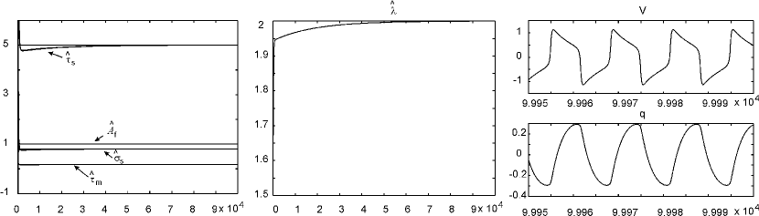
Figure 3: Left panel: estimates of parameters $\tau_{m},\tau_{s},\sigma_{s},A_{f}$ as functions of $t$. Middle panel: estimate of ${\lambda}$. Right panel: true values of $V$ and $q$ and their estimates in the end of the simulation.

6 Conclusion

In this work we provided an extension of the observer design for systems nonlinear in parameter Tyukin et al. (2013). The extension allows to account for parametric constraints in the form of equalities. The approach presented enables inclusion of additional information about location of true parameter values and as such helps to improve robustness of the estimation procedure.

Appendix

Proof of Lemma 4. According to condition (4) we can conclude that that $h(t_{0})\geq 0$. Let us introduce a strictly decreasing sequence: $\{\sigma_{i}\},\ i=0,1,\dots,\ \sigma_{i}=(1/\kappa)^{i},\ \kappa\in(1,\infty)$. Further, let $\{t_{i}\},\ i=1,\dots,\ t_{1}<t_{2}<\cdots<t_{n}<\cdots$ be an ordered infinite sequence of time instants such that

$$h(t_{i})=\sigma_{i}h(t_{0}).$$ (29)

If the latter assumption does not hold then one can immediately conclude that $h(t)$ is bounded from below by $0$ for $t\geq t_{0}$; it is also bounded from above by $h(t_{0})$, for $t\geq t_{0}$. Hence $h(t)$ is bounded for all $t\geq t_{0}$. Moreover, in accordance with (22), trajectory $\mathbf{x}(t)$ is bounded for all $t\geq t_{0}$, and nothing remains to be proven.

We wish to show that if (24), (4), and (29) then

$$h(t)\rightarrow 0\Rightarrow t\rightarrow\infty.$$ (30)

In order to do so consider the time differences $T_{i}=t_{i}-t_{i-1}$. It is clear from (22) and (23) that

$$\begin{split}&T_{i}D_{\gamma}(\max_{\tau\in[t_{i-1},t_{i}]}\|\mathbf{x}(\tau)+\mathbf{d}(\tau)\|_{\varepsilon}+Mh(t_{0})\sigma_{i-1})\\ &\geq h(t_{0})(\sigma_{i-1}-\sigma_{i}).\end{split}$$ (31)

Since

$$\max_{\tau\in[t_{i-1},t_{i}]}\|\mathbf{x}(\tau)+\mathbf{d}(\tau)\|_{\varepsilon}=\|\mathbf{x}(\tau)+\mathbf{d}(\tau)\|_{\infty,[t_{i-1},t_{i}]}-\varepsilon$$

if $\|\mathbf{x}(\tau)+\mathbf{d}(\tau)\|_{\infty,[t_{i-1},t_{i}]}>\varepsilon$, and $\max_{\tau\in[t_{i-1},t_{i}]}\|\mathbf{x}(\tau)+\mathbf{d}(\tau)\|_{\varepsilon}=0$ overwise, we can see from (31) that

$$T_{i}\geq\left\{\begin{array}[]{l}\frac{h(t_{0})(\sigma_{i-1}-\sigma_{i})}{D_{\gamma}(\|\mathbf{x}(\tau)+\mathbf{d}(\tau)\|_{\infty,[t_{i-1},t_{i}]}-\varepsilon+Mh(t_{0})\sigma_{i-1})},\\ \ \ \ \ \ \ |\|\mathbf{x}(\tau)+\mathbf{d}(\tau)\|_{\infty,[t_{i-1},t_{i}]}>\varepsilon;\\ \frac{\sigma_{i-1}-\sigma_{i}}{D_{\gamma}M\sigma_{i-1}},\ \|\mathbf{x}(\tau)+\mathbf{d}(\tau)\|_{\infty,[t_{i-1},t_{i}]}\leq\varepsilon.\end{array}\right.$$ (32)

Pick

$$\tau^{\ast}=\beta^{-1}\left({d}/{\kappa}\right),\ d\in(0,1),$$ (33)

and select the value of $D_{\gamma}$ such that (4) holds. Consider two cases: a) $\|\mathbf{x}(\tau)+\mathbf{d}(\tau)\|_{\infty,[t_{i-1},t_{i}]}-\varepsilon\leq 0$ and b) $\|\mathbf{x}(\tau)+\mathbf{d}(\tau)\|_{\infty,[t_{i-1},t_{i}]}-\varepsilon>0$. With respect to case a) we immediately observe that $T_{i}\geq\tau^{\ast}$ for all $i$.

Consider case b). Given that $\|\mathbf{x}(\tau)+\mathbf{d}(\tau)\|_{\infty,[t_{0},t_{1}]}-\varepsilon\leq\beta(0)\|\mathbf{x}(t_{0})\|+ch(t_{0})+\Delta+\Delta_{d}-\varepsilon$, conditions (4), (24), and (33) imply $D_{\gamma}\leq\frac{\kappa-1}{\kappa}\frac{h(t_{0})}{\beta(0)\|\mathbf{x}(t_{0})\|+(c+M)|h(t_{0})|}\frac{1}{\tau^{\ast}}\leq\frac{h(t_{0})(\sigma_{0}-\sigma_{1})}{(\|\mathbf{x}(\tau)+\mathbf{d}(\tau)\|_{\infty,[t_{0},t_{1}]}-\varepsilon+M|h(t_{0})|)}\frac{1}{\tau^{\ast}}$. This, as follows from (32), guarantees that $T_{1}\geq\tau^{\ast}$. Suppose that there is an $i\geq 2$ such that $T_{j}\geq\tau^{\ast}$ for all $1\leq j\leq i-1$. We will now show that the following implication holds $T_{i-1}\geq\tau^{\ast}\Rightarrow T_{i}\geq\tau^{\ast}$. This will ensure that (30) is satisfied and, consequently, that the lemma hold. Consider $\|\mathbf{x}(\tau)\|_{\infty,[t_{i-1},t_{i}]}$; (22) and (29) imply that: $\|\mathbf{x}(\tau)\|_{\infty,[t_{i-1},t_{i}]}\leq\beta(0)\|\mathbf{x}(t_{i-1})\|+c\sigma_{i-1}h(t_{0})+\Delta$. Estimating $\|\mathbf{x}(t_{i-1})\|$ from above, according to (22), results in

$$\begin{split}&\|\mathbf{x}(\tau)\|_{\infty,[t_{i-1},t_{i}]}\leq\beta(0)[\beta(T_{i-1})\|\mathbf{x}(t_{i-2})\|+c\sigma_{i-2}h(t_{0})]\\ &+\beta(0)\Delta+ch(t_{0})\sigma_{i-1}+\Delta\leq\beta(0)\beta(\tau^{\ast})\|\mathbf{x}(t_{i-2})\|+P_{1},\end{split}$$

where $P_{1}=\beta(0)c\sigma_{i-2}h(t_{0})+c\sigma_{i-1}h(t_{0})+\beta(0)\Delta+\Delta$. Invoking (22) in order to express an upper bound for $\|\mathbf{x}(t_{i-2})\|$ in terms of $\|\mathbf{x}(t_{i-3})\|$ leads to

$$\begin{split}&\|\mathbf{x}(\tau)\|_{\infty,[t_{i-1},t_{i}]}\leq\beta(0)\beta^{2}(\tau^{\ast})\|\mathbf{x}(t_{i-3})\|+P_{2},\end{split}$$

where $P_{2}=ch(t_{0})\beta(0)[\beta(\tau^{\ast})\sigma_{i-3}+\sigma_{i-2}]+c\sigma_{i-1}h(t_{0})+\beta(0)[\beta(\tau^{\ast})\Delta+\Delta]+\Delta$, and

$$\begin{split}&\|\mathbf{x}(\tau)\|_{\infty,[t_{i-1},t_{i}]}\leq\beta(0)\beta^{3}(\tau^{\ast})\|\mathbf{x}(t_{i-4})\|+P_{3},\end{split}$$

where

$$\begin{array}[]{l}P_{3}=ch(t_{0})\beta(0)[\beta^{2}(\tau^{\ast})\sigma_{i-4}+\beta(\tau^{\ast})\sigma_{i-3}+\sigma_{i-2}]\\ +c\sigma_{i-1}h(t_{0})+\Delta\beta(0)[\beta(\tau^{\ast})^{2}+\beta(\tau^{\ast})+1]+\Delta\\ =ch(t_{0})\beta(0)\big{[}\sum_{j=0}^{2}\beta^{j}(\tau^{\ast})\sigma_{i-j-2}\big{]}+ch(t_{0})\sigma_{i-1}\\ +\Delta\beta(0)\big{[}\sum_{j=0}^{2}\beta^{j}(\tau^{\ast})\big{]}+\Delta.\end{array}$$

After $i-1$ steps we obtain

$$\begin{split}\|\mathbf{x}(\tau)\|_{\infty,[t_{i-1},t_{i}]}&\leq\beta(0)\beta^{i-1}(\tau^{\ast})\|\mathbf{x}(t_{0})\|+P_{i-1},\end{split}$$ (34)

where

$$\begin{array}[]{l}P_{i-1}=ch(t_{0})\beta(0)\big{[}\sum_{j=0}^{i-2}\beta^{j}(\tau^{\ast})\sigma_{i-j-2}\big{]}+ch(t_{0})\sigma_{i-1}\\ +\Delta\beta(0)\big{[}\sum_{j=0}^{i-2}\beta^{j}(\tau^{\ast})\big{]}+\Delta.\end{array}$$

The values of $T_{i}$, as follows from (32), satisfy:

$$T_{i} \geq \frac{\sigma_{i-1}-\sigma_{i}}{\sigma_{i-1}}h(t_{0})\big{[}D_{\gamma}\sigma_{i-1}^{-1}\big{(}\|\mathbf{x}(\tau)+\mathbf{d}(\tau)\|_{\infty,[t_{i-1},t_{i}]}-\varepsilon$$ (35)

$$+Mh(t_{0})\sigma_{i-1}\big{)}\big{]}^{-1}.$$

Consider

$$\sigma_{i-1}^{-1}\left(\|\mathbf{x}(\tau)+\mathbf{d}(\tau)\|_{\infty,[t_{i-1},t_{i}]}-\varepsilon+Mh(t_{0})\sigma_{i-1}\right).$$

Taking (34) into account we derive that:

$$\begin{array}[]{l}\sigma_{i-1}^{-1}\left(\|\mathbf{x}(\tau)+\mathbf{d}(\tau)\|_{\infty,[t_{i-1},t_{i}]}-\varepsilon+Mh(t_{0})\sigma_{i-1}\right)\\ \leq\beta(0)\beta^{i-1}(\tau^{\ast})\kappa^{i-1}\|\mathbf{x}(t_{0})\|+k^{i-1}P_{i-1}+k^{i-1}\Delta_{d}\\ -k^{i-1}\varepsilon+Mh(t_{0})=\beta(0)\beta^{i-1}(\tau^{\ast})\kappa^{i-1}\|\mathbf{x}(t_{0})\|\\ +ch(t_{0})\beta(0)\kappa\big{[}\sum_{j=0}^{i-2}\beta^{j}(\tau^{\ast})\kappa^{j}\big{]}+(c+M)h(t_{0})\\ +\kappa^{i-1}\big{[}\Delta\big{(}\beta(0)\sum_{j=0}^{i-2}\beta^{j}(\tau^{\ast})+1\big{)}+\Delta_{d}-\varepsilon\big{]}.\end{array}$$

Noticing that $\tau^{\ast}$ is chosen in accordance with (33) one can therefore obtain:

$$\begin{array}[]{l}\sigma_{i-1}^{-1}\left(\|\mathbf{x}(\tau)+\mathbf{d}(\tau)\|_{\infty,[t_{i-1},t_{i}]}-\varepsilon+Mh(t_{0})\sigma_{i-1}\right)\\ \leq\beta(0)\|\mathbf{x}(t_{0})\|+(c+M)h(t_{0})+ch(t_{0})\beta(0)\kappa\sum_{j=0}^{i-2}d^{j}+\\ \kappa^{i-1}\big{[}\Delta\big{(}\beta(0)\sum_{j=0}^{i-2}\frac{d}{\kappa}^{j}+1\big{)}+\Delta_{d}-\varepsilon\big{]}\\ \leq\beta(0)\|\mathbf{x}(t_{0})\|+h(t_{0})\big{(}c\big{(}1+\frac{\beta(0)\kappa}{1-d}\big{)}+M\big{)}+\\ k^{i-1}\big{[}\Delta\big{(}\frac{\beta(0)}{1-d/k}+1\big{)}+\Delta_{d}-\varepsilon\big{]}.\end{array}$$

Condition (24) implies that $\Delta\left(\frac{\beta(0)}{1-d/k}+1\right)+\Delta_{d}-\varepsilon\leq 0$. Hence $\sigma_{i-1}^{-1}\left(\|\mathbf{x}(\tau)+\mathbf{d}(\tau)\|_{\infty,[t_{i-1},t_{i}]}-\varepsilon+Mh(t_{0})\sigma_{i-1}\right)\leq\beta(0)\|\mathbf{x}(t_{0})\|+h(t_{0})\left(c\left(1+\frac{\beta(0)\kappa}{1-d}\right)+M\right)$. Substituting the latter estimate into (35) and using (4) yields $T_{i}\geq\tau^{\ast}$ as required. Therefore $T_{i}\geq\tau^{\ast}$ for all $i\geq 1$, and (30) holds. Thus the trajectory $h(t)$ is bounded from above and below, and hence so is the trajectory $\mathbf{x}(t)$. $\square$

References

- Bastin and Gevers (1988) Bastin, G. and Gevers, M. (1988). Stable adaptive observers for nonlinear time-varying systems. IEEE Trans. on Automatic Control, 33(7), 650–658.
- Besancon (2000) Besancon, G. (2000). Remarks on nonlinear adaptive observer design. Systems and Control Letters, 41, 271–280.
- Farza et al. (2009) Farza, M., M’Saad, M., Maatoung, T., and Kamoun, M. (2009). Adaptive observers for nonlinearly parameterized class of nonlinear systems. Automatica, 45, 2292–2299.
- Grip et al. (2011) Grip, H., Saberi, A., and Johansen, T. (2011). Estimation of states and parameters for linear systems with nonlinearly parameterized perturbations. Systems and Control Letters, 60(9), 771–777.
- Krstic et al. (1995) Krstic, M., Kanellakopoulos, I., and Kokotovic, P. (1995). Nonlinear and Adaptive Control Design. Wiley and Sons Inc.
- Loria and Panteley (2003) Loria, A. and Panteley, E. (2003). Uniform exponential stability of linear time-varying systems: revisited. Systems and Control Letters, 47(1), 13–24.
- Marino (1990) Marino, R. (1990). Adaptive observers for single output nonlinear systems. IEEE Trans. Automatic Control, 35(9), 1054–1058.
- Marino and Tomei (1993) Marino, R. and Tomei, P. (1993). Global adaptive output-feedback control of nonlinear systems, part I: Linear parameterization. IEEE Trans. Automatic Control, 38(1), 17–32.
- Marino and Tomei (1995) Marino, R. and Tomei, P. (1995). Adaptive observers with arbitrary exponential rate of convergence for nonlinear systems. IEEE Trans. Automatic Control, 40(7), 1300–1304.
- Rowat and Selverston (1993) Rowat, P. and Selverston, A. (1993). Modeling the gastric mill central pattern generator with a relaxation-oscillator network. J. Neuro-physiol., 70(3), 1030–1053.
- Tyukin et al. (2013) Tyukin, I., Steur, E., Nijmeijer, H., and van Leeuwen, C. (2013). Adaptive observers and parameter estimation for a class of systems nonlinear in the parameters. Automatica, 49(8), 2409–2423.