Nonparametric tests for detecting breaks in the jump behaviour of a time-continuous process

Abstract

This paper is concerned with tests for changes in the jump behaviour of a time-continuous process. Based on results on weak convergence of a sequential empirical tail integral process, asymptotics of certain tests statistics for breaks in the jump measure of an Itō semimartingale are constructed. Whenever limiting distributions depend in a complicated way on the unknown jump measure, empirical quantiles are obtained using a multiplier bootstrap scheme. An extensive simulation study shows a good performance of our tests in finite samples.

Keywords and Phrases: Change points; Lévy measure; multiplier bootstrap; sequential empirical processes; weak convergence.

AMS Subject Classification: 60F17, 60G51, 62G10.

1 Introduction

Recent years have witnessed a growing interest in statistical tools for high-frequency observations of time-continuous processes. With a view on finance, the seminal paper by Delbaen and Schachermayer (1994) suggests to model such a process using Itō semimartingales, say $X$, which is why most research has focused on the estimation of (or on tests concerned with) its characteristics. Particular interest has been paid to integrated volatility or the entire quadratic variation, mostly adapting parametric procedures based on normal distributions, as the continuous martingale part of an Itô semimartingale is nothing but a time-changed Brownian motion. For an overview on methods in this field see the recent monographs by Jacod and Protter (2012) and Aït-Sahalia and Jacod (2014).

Still less popular is inference on the jump behaviour only, even though empirical research shows a strong evidence supporting the presence of a jump component within $X$; see e.g. Aït-Sahalia and Jacod (2009b) or Aït-Sahalia and Jacod (2009a). In this work, we will address the question whether the jump behaviour of $X$ is time-invariant. Corresponding tests, commonly referred to as change point tests, are well known in the framework of discrete time series, but have recently also been extended to time-continuous processes; see e.g. Lee et al. (2006) on changes in the drift or Iacus and Yoshida (2012) on changes in the volatility function of $X$. However, to the best of our knowledge, no procedures are available for detecting breaks in the jump component.

Suppose that we observe an Itō semimartingale $X$ which admits a decomposition of the form

$$X_{t}=X_{0}+\int_{0}^{t}b_{s}\,ds+\int_{0}^{t}\sigma_{s}\,dW_{s}+\int_{0}^{t}\int_{\mathbb{R}}u1_{\{|u|\leq 1\}}(\mu-\bar{\mu})(ds,du)\\ +\int_{0}^{t}\int_{\mathbb{R}}u1_{\{|u|>1\}}\mu(du,dz),$$ (1.1)

where $W$ is a standard Brownian motion, $\mu$ is a Poisson random measure on $\mathbb{R}^{+}\times\mathbb{R}$, and the predictable compensator $\bar{\mu}$ satisfies $\bar{\mu}(ds,du)=ds\>\nu_{s}(du)$. As a fairly general structural assumption, we allow the characteristics of $X$, i.e. $b_{t},\sigma_{t}$ and $\nu_{t},$ to depend deterministically on time. Recall that $\nu_{t}$ can be interpreted as a local Lévy measure, such that

$$\int_{\mathbb{R}}(1\wedge|u|^{2})\nu_{t}(du)<\infty$$

for each $t$ and $\nu_{t}(A)$ denotes the average number of jumps that fall into the set $A$ over a unit time interval.

Now, we assume that we have data from the process in a high-frequency setup. Precisely, at stage $n\in\mathbb{N}$, we are able to observe realizations of the process $X$ at the equidistant times $i\Delta_{n}$ for $i=1,\ldots,n$, where the mesh $\Delta_{n}\rightarrow 0$, while $n\Delta_{n}\rightarrow\infty$. In this situation we want to test the null hypothesis that the jump behaviour of the process is the same for all $n$ observations, i.e. there exists some measure $\nu$ such that $\nu_{t}(dz)=\nu(dz)$ for all $t$, against alternatives involving the non-constancy of $\nu_{t}$. For instance, one might consider an alternative consisting of one break point, i.e. there exists some $\theta_{0}\in(0,1)$ and two Lévy measures $\nu_{1}$, $\nu_{2}$ such that the process behind the first $\lfloor n\theta_{0}\rfloor$ observations has Lévy measure $\nu_{1}$ and the remaining $n-\lfloor n\theta_{0}\rfloor$ observations are taken from a process with Lévy measure $\nu_{2}$. The restriction to a deterministic drift and volatility in (1.1) is merely technical here, as it allows to use empirical process theory for independent observations later. An argument similar to that in Section 5.3 in Bücher and Vetter (2013) proves that one might as well work with random coefficients $b$ and $\sigma$.

Throughout the work, we will restrict ourselves to positive jumps only. Thus, for $z>0$, let $U(z):=\nu([z,\infty))$ denote the tail integral (or spectral measure; see Rüschendorf and Woerner, 2002) associated with $\nu$, which determines the jump measure uniquely. For $\ell_{1},\ell_{2}\in\{1,\dots,n\}$ such that $\ell_{1}<\ell_{2}$, define

$$U_{\ell_{1}:\ell_{2}}(z):=\frac{1}{(\ell_{2}-\ell_{1}+1)\Delta_{n}}\sum\limits_{j=\ell_{1}}^{\ell_{2}}\mathtt{1}_{\{\Delta_{j}^{n}X\geq z\}}\quad(z>0),$$

with $\Delta_{j}^{n}X:=X_{j\Delta_{n}}-X_{(j-1)\Delta_{n}}$, which serves as an empirical tail integral based on the increments $\Delta_{\ell_{1}}^{n}X,\dots,\Delta_{\ell_{2}}^{n}X$. If $X$ is a Lévy process with a Lévy measure $\nu$ not changing in time, Figueroa-Lopez (2008) illustrated that $U_{1:n}(z)$ is a suitable estimator for the tail integral $U(z)$ in the sense that, under regularity conditions, $U_{n}(z)$ is $L^{2}$-consistent for $U(z)$. Following the approach in Inoue (2001), it is therefore likely that we can base tests for $H_{0}$ on suitable functionals of the process

$$D_{n}(\theta,z):=U_{1:\lfloor n\theta\rfloor}(z)-U_{(\lfloor n\theta\rfloor+1):n}(z),$$

where $\theta\in[0,1]$ and $z>0$. Under the null hypothesis, this expression can be expected to converge to $0$ for all $\theta\in[0,1]$ and $z>0$, whereas under alternatives, for instance those involving a change at $\theta_{0}$ as described before, $D_{n}(\theta_{0},z)$ should converge to an expression which is non-zero.

More precisely, we will consider the following standardized version of $D_{n}$, namely

$$\mathbb{T}_{n}(\theta,z):=\sqrt{n\Delta_{n}}\lambda_{n}(\theta)\left\{U_{1:\lfloor n\theta\rfloor}(z)-U_{(\lfloor n\theta\rfloor+1):n}(z)\right\}$$ (1.2)

for $\theta\in[0,1]$ and $z>0$, where $\lambda_{n}(\theta)=\frac{\lfloor n\theta\rfloor}{n}\frac{n-\lfloor n\theta\rfloor}{n}$. An appropriate functional allowing to test the hypothesis of a constant Lévy measure is for instance given by a Kolmogorov-Smirnov statistic of the form

$$T_{n}^{(\varepsilon)}:=\sup\limits_{\theta\in[0,1]}\sup\limits_{z\geq\varepsilon}|\mathbb{T}_{n}(\theta,z)|,\quad(\varepsilon>0).$$ (1.3)

The null hypothesis of no change in the Lévy measure is rejected for large values of $T_{n}^{\scriptscriptstyle(\varepsilon)}$. The restriction to jumps larger than $\varepsilon$ is important, since there might be infinitely many of arbitrary small size.

The limiting distribution of the previously mentioned test statistic will turn out to depend in a complicated way on the unknown Lévy measure $\nu$. Therefore, corresponding quantiles are not easily accessible and must be obtained by suitable bootstrap approximations. Following related ideas for detecting breaks within multivariate empirical distribution functions (Inoue, 2001), we opt for using empirical counterparts based on a multiplier bootstrap scheme, frequently also referred to as wild or weighted bootstrap. The approach essentially consists of multiplying each indicator within the respective empirical tail integrals with an additional, independent and standardized multiplier. The underlying empirical process theory is for instance summarized in the monograph Kosorok (2008).

The remaining part of this paper is organized as follows: the derivation of a functional weak convergence result for the process $\mathbb{T}_{n}$ under the null hypothesis is the content of Section 2. The asymptotic properties of $T_{n}^{\scriptscriptstyle(\varepsilon)}$ can then easily be derived from the continuous mapping theorem. Section 3 is concerned with the approximation of the limiting distribution using the previously described multiplier bootstrap scheme. In Section 4, we discuss the formal derivation of several tests for a time-homogeneous jump behaviour, whereas an extensive simulation study is presented in Section 5. All proofs are deferred to the Appendix, which is Section 6.

2 Functional weak convergence of the sequential empirical tail integral

In this section, we derive a functional weak convergence result for the process $\mathbb{T}_{n}$ defined in (1.2). For that purpose, we have to introduce an appropriate function space. We set $\mathbb{A}:=[0,1]\times(0,\infty)$ and let $\mathcal{B}_{\infty}(\mathbb{A})$ denote the space of all functions $f\colon\mathbb{A}\rightarrow\mathbb{R}$ which are bounded on every set $A\subset\mathbb{A}$ for which the projection onto the second coordinate, $p_{2}(A)=\{z\in(0,\infty)\mid\exists\theta\in[0,1]\text{ such that }(\theta,z)\in A\}$, is bounded away from $0$. Moreover, for $k\in\mathbb{N}$, we define $A_{k}:=[0,1]\times[k^{-1},\infty)\subset\mathbb{A}$, and, for $f,g\in\mathcal{B}_{\infty}(\mathbb{A})$, we set

$$d(f,g):=\sum\limits_{k=1}^{\infty}2^{-k}(\|f-g\|_{A_{k}}\wedge 1),$$

where $\|f-g\|_{A_{k}}=\sup\{|f(x)-g(x)|\,:\,x\in A_{k}\}.$ Note that $d$ defines a metric on $\mathcal{B}_{\infty}(\mathbb{A})$ which induces the topology of uniform convergence on all sets $A$ such that its projection $p_{2}(A)$ is bounded away from $0$, i.e. a sequence of functions converges with respect to $d$ if and only if it converges uniformly on each $A_{k}$ (Van der Vaart and Wellner, 1996, Chapter 1.6).

Furthermore to establish our results on weak convergence under the null hypothesis, we impose the following conditions.

Condition 2.1.

$X$ is an Itō semimartingale with the representation in (1.1) such that

1. The drift $b_{t}$ and the volatility $\sigma_{t}$ are càglàd, bounded and deterministic.

2. There exists some Lévy measure $\nu$ such that $\nu_{t}\equiv\nu$ for all $t\in\mathbb{R}_{+}$.

3. $X$ has only positive jumps, that is, the jump measure $\nu$ is supported on $(0,\infty)$.

4. $\nu$ is absolutely continuous with respect to the Lebesgue measure on $(0,\infty)$. Its density $h=d\nu/d\lambda$, called Lévy density, is differentiable with derivative $h^{\prime}$ and satisfies

   $$\|h\|_{M_{k}}+\|h^{\prime}\|_{M_{k}}<\infty$$

   for all $k\in\mathbb{N}$ with $M_{k}:=[k^{-1},\infty)$. ∎

The next lemma is essential for the weak convergence results. Similar statements can be found in Figueroa-Lopez and Houdre (2009), with slightly stronger assumptions on $h$, and in Bücher and Vetter (2013) in the bivariate case.

Lemma 2.2.

Let $X$ be an Itō semimartingale that satisfies Condition 2.1. Let further be $\delta>0$ fixed. If $X_{0}=0$, then there exist constants $K=K(\delta)>0$ and $t_{0}=t_{0}(\delta)>0$, depending on the bounds on the characteristics in Condition 2.1(a), such that the inequality

$$\left|\mathbb{P}(X_{t}\in[z,\infty))-t\nu([z,\infty))\right|<Kt^{2}$$

holds for all $z\geq\delta$ and all $0<t<t_{0}$.

Remark 2.3.

If $X$ is an Itō semimartingale satisfying Condition 2.1, then Lemma 2.2 implies immediately that we have

$$\sup\limits_{s\in\mathbb{R}_{+}}\left|\mathbb{P}(X_{s+t}-X_{s}\in[z,\infty))-t\nu([z,\infty))\right|\leq Kt^{2}$$

as well. To see this note that, for each fixed $s\in\mathbb{R}_{+}$, the Itō semimartingale $(Y^{\scriptscriptstyle(s)}_{t})_{t\in\mathbb{R}_{+}}$ with $Y^{\scriptscriptstyle(s)}_{t}:=X_{s+t}-X_{s}$ satisfies Condition 2.1, and its characteristics have the same bounds as the characteristics of $X$. ∎

The limiting behaviour of the process $\mathbb{T}_{n}$ can be deduced from the next theorem, which is a result for weak convergence of a sequential empirical tail integral process. For $\theta\in[0,1]$ and $z>0$ set

$$U_{n}(\theta,z):=\frac{\lfloor n\theta\rfloor}{n}U_{1:\lfloor n\theta\rfloor}(z)=\frac{1}{k_{n}}\sum\limits_{j=1}^{\lfloor n\theta\rfloor}\mathtt{1}_{\{\Delta_{j}^{n}X\geq z\}},$$ (2.1)

where $k_{n}:=n\Delta_{n}$ and denote its standardized version by

$$\mathbb{G}_{n}(\theta,z):=\sqrt{k_{n}}\{U_{n}(\theta,z)-\mathbb{E}U_{n}(\theta,z)\}.$$ (2.2)

Obviously, the sample paths of $U_{n}(\theta,z)$ are elements of $\mathcal{B}_{\infty}(\mathbb{A})$.

Theorem 2.4.

Let $X$ be an Itō semimartingale that satisfies Condition 2.1. Furthermore, assume that the observation scheme has the properties:

$$\Delta_{n}\rightarrow 0,\quad\text{ }\quad n\Delta_{n}=k_{n}\rightarrow\infty.$$

Then, $\mathbb{G}_{n}\rightsquigarrow\mathbb{G}$ in $(\mathcal{B}_{\infty}(\mathbb{A}),d)$, where $\mathbb{G}$ is a tight mean zero Gaussian process with covariance

$$H(\theta_{1},z_{1};\theta_{2},z_{2}):=\mathbb{E}[\mathbb{G}(\theta_{1},z_{1})\mathbb{G}(\theta_{2},z_{2})]=(\theta_{1}\wedge\theta_{2})\times\nu([z_{1}\vee z_{2},\infty))$$

for $(\theta_{1},z_{1}),(\theta_{2},z_{2})\in\mathbb{A}$. The sample paths of $\mathbb{G}$ are almost surely uniformly continuous on each $A_{k}$ $(k\in\mathbb{N}$) with respect to the semimetric

$$\rho(\theta_{1},z_{1};\theta_{2},z_{2}):=\big{\{}(\theta_{1}\wedge\theta_{2})\nu([z_{1}\wedge z_{2},z_{1}\vee z_{2}))+\left|\theta_{1}-\theta_{2}\right|\nu([z_{I(\theta_{1},\theta_{2})},\infty))\big{\}}^{\frac{1}{2}}$$

with $I(\theta_{1},\theta_{2}):=1+\mathtt{1}_{\{\theta_{1}\leq\theta_{2}\}}.$

Note that we have centered $U_{n}(\theta,z)$ around its expectation in (2.2). In most applications, however, we are interested in estimating functionals of the jump measure, and according to Lemma 2.2 we need stronger conditions then. Precisely, we consider the process

$$\tilde{\mathbb{G}}_{n}(\theta,z):=\sqrt{k_{n}}\{U_{n}(\theta,z)-\theta\nu([z,\infty))\}$$

and get, as an immediate consequence of the previous two results, the following sequential generalization of Theorem 4.2 of Bücher and Vetter (2013).

Corollary 2.5.

Let $X$ be an Itō semimartingale that satisfies Condition 2.1. If the observation scheme meets the conditions

$$\Delta_{n}\rightarrow 0,\quad\text{ }\quad n\Delta_{n}=k_{n}\rightarrow\infty,\quad\text{ }\quad\sqrt{k_{n}}\Delta_{n}\rightarrow 0,$$

then $\tilde{\mathbb{G}}_{n}\rightsquigarrow\mathbb{G}$ in $(\mathcal{B}_{\infty}(\mathbb{A}),d)$, where $\mathbb{G}$ denotes the Gaussian process from Theorem 2.4.

A further consequence of Theorem 2.4 is the desired weak convergence of the process $\mathbb{T}_{n}$, which was defined in (1.2), under the null hypothesis.

Theorem 2.6.

Suppose the assumptions of Corollary 2.5 are satisfied. Then, the process $\mathbb{T}_{n}$ defined in (1.2) converges weakly to $\mathbb{T}$ in $(\mathcal{B}_{\infty}(\mathbb{A}),d)$, where

$$\mathbb{T}(\theta,z)=\mathbb{G}(\theta,z)-\theta\mathbb{G}(1,z)$$

for $(\theta,z)\in\mathbb{A}$, and where $\mathbb{G}$ denotes the limit process in Theorem 2.4. $\mathbb{T}$ is a tight mean zero Gaussian process with covariance function

$$\hat{H}(\theta_{1},z_{1};\theta_{2},z_{2}):=\mathbb{E}\{\mathbb{T}(\theta_{1},z_{1})\mathbb{T}(\theta_{2},z_{2})\}=\{(\theta_{1}\wedge\theta_{2})-\theta_{1}\theta_{2}\}\nu([z_{1}\vee z_{2},\infty)).$$

Using the continuous mapping theorem, we are now able to derive the weak convergence of various statistics allowing for the detection of breaks in the jump behaviour. The following corollary treats the statistic $T_{n}^{(\varepsilon)}$ defined in (1.3).

Corollary 2.7.

Under the assumptions of Corollary 2.5 we have, for each $\varepsilon>0$,

$$T_{n}^{(\varepsilon)}\rightsquigarrow T^{(\varepsilon)}:=\sup\limits_{0\leq\theta\leq 1}\sup\limits_{z\geq\varepsilon}|\mathbb{T}(\theta,z)|,$$

where $\mathbb{T}$ is the limit process defined in Theorem 2.6.

The covariance function of the limit process in Theorem 2.6 depends on the Lévy measure of the underlying process, which is usually unknown in applications. If one only wants to detect changes in the tail integral of the Lévy measure at a fixed point $z_{0}$, the following proposition deals with the simple transformation

$$\mathbb{V}_{n}^{(z_{0})}(\theta):=\frac{\mathbb{T}_{n}(\theta,z_{0})}{\sqrt{U_{1:n}(z_{0})}}\mathtt{1}_{\{U_{1:n}(z_{0})>0\}}$$

of $\mathbb{T}_{n}$ which yields a pivotal limiting distribution.

Proposition 2.8.

Let $X$ be an Itō semimartingale that satisfies Condition 2.1. Moreover, let $z_{0}>0$ be a real number with $\nu([z_{0},\infty))>0$ and suppose that the underlying observation scheme meets the assumptions from Corollary 2.5. Then, $\mathbb{V}_{n}^{(z_{0})}\rightsquigarrow\mathbb{B}$ in $\ell^{\infty}([0,1])$, where $\mathbb{B}$ denotes a standard Brownian bridge. As a consequence,

$$V_{n}^{(z_{0})}:=\sup\limits_{\theta\in[0,1]}|\mathbb{V}_{n}^{(z_{0})}(\theta)|\rightsquigarrow\sup\limits_{\theta\in[0,1]}\mathbb{|}B(\theta)|,$$

the limiting distribution being also known as the Kolmogorov-Smirnov distribution.

Remark 2.9.

We have derived the previous results under somewhat simplified assumptions on the observation scheme in order to keep the presentation rather simple. A more realistic setting could involve additional microstructure noise effects or might rely on non-equidistant data. In both cases, standard techniques still yield similar results.

For example, in case of noisy observations, Vetter (2014) has shown that a particular de-noising technique allows for virtually the same results on weak convergence as for the plain $U_{n}(\theta,z)$ in the case without noise. For non-equidistant data, the limiting covariance functions $H$ and $\hat{H}$ in general depend on the sampling scheme. The latter effect is well-known from high-frequency statistics in the case of volatility estimation; see e.g. Mykland and Zhang (2012). ∎

3 Bootstrap approximations for the sequential empirical tail integral

We have seen in Corollary 2.7 that the distribution of the limit $\mathbb{T}$ of the process $\mathbb{T}_{n}$ depends in a complicated way on the unknown Lévy measure of the underlying process. However, we need the quantiles of $\mathbb{T}$ or at least good approximations for them to obtain a feasible test procedure. Typically, one uses resampling methods to solve this problem.

Probably the most natural way to do so is to use $U_{1:n}(z)$ in order to obtain an estimator $\hat{\nu}_{n}$ for the Lévy measure first, and to draw a large number of independent samples of an Itō semimartingale with Lévy measure $\hat{\nu}_{n}$ then, possibly with estimates for drift and volatility as well. Based on each sample, one might then compute the test statistic $\mathbb{T}_{n}$, and by doing so one obtains empirical quantiles for $\mathbb{T}$.

However, from a computational side, such a method is computationally expensive since one has to generate independent Itō semimartingales for each stage within the bootstrap algorithm. Therefore we have decided to work with an alternative bootstrap method based on multipliers, where one only needs to generate $n$ i.i.d. random variables with mean zero and variance one (see also Inoue, 2001, who used a similar approach in the context of empirical processes).

Precisely, the situation now is as follows: The bootstrapped processes, say $\hat{Y}_{n}=\hat{Y}_{n}(X_{1},\ldots,X_{n},\xi_{1},\ldots,\xi_{n})$, will depend on some random variables $X_{1},\ldots,X_{n}$ and on some random weights $\xi_{1},\ldots,\xi_{n}$. The $X_{1},\ldots,X_{n}$, that we consider as collected data, are defined on a probability space $(\Omega_{X},\mathcal{A}_{X},\mathbb{P}_{X})$. The random weights $\xi_{1},\ldots,\xi_{n}$ are defined on a distinct probability space $(\Omega_{\xi},\mathcal{A}_{\xi},\mathbb{P}_{\xi})$. Thus, the bootstrapped processes live on the product space $(\Omega,\mathcal{A},\mathbb{P}):=(\Omega_{X},\mathcal{A}_{X},\mathbb{P}_{X})\otimes(\Omega_{\xi},\mathcal{A}_{\xi},\mathbb{P}_{\xi})$. The following notion of conditional weak convergence will be essential. It can be found in Kosorok (2008) on pp. 19–20.

Definition 3.1.

Let $\hat{Y}_{n}=\hat{Y}_{n}(X_{1},\ldots,X_{n};\xi_{1},\ldots,\xi_{n})\colon(\Omega,\mathcal{A},\mathbb{P})\rightarrow\mathbb{D}$ be a (bootstrapped) element in some metric space $\mathbb{D}$ depending on some random variables $X_{1},\ldots,X_{n}$ and some random weights $\xi_{1},\ldots,\xi_{n}$. Moreover, let $Y$ be a tight, Borel measurable map into $\mathbb{D}$. Then $\hat{Y}_{n}$ converges weakly to $Y$ conditional on the data $X_{1},X_{2},\ldots$ in probability, notationally $\hat{Y}_{n}{\,{\rightsquigarrow_{\xi}}\ }Y$, if and only if

1. $\sup\limits_{f\in\text{BL}_{1}(\mathbb{D})}|\mathbb{E}_{\xi}f(\hat{Y}_{n})-\mathbb{E}f(Y)|\stackrel{{\scriptstyle\scriptscriptstyle\mathbb{P}^{*}}}{{\rightarrow}}0,$

2. $\mathbb{E}_{\xi}f(\hat{Y}_{n})^{\ast}-\mathbb{E}_{\xi}f(\hat{Y}_{n})_{\ast}\stackrel{{\scriptstyle\scriptscriptstyle\mathbb{P}^{*}}}{{\rightarrow}}0$ for all $f\in\text{BL}_{1}(\mathbb{D}).$

Here, $\mathbb{E}_{\xi}$ denotes the conditional expectation over the weights $\xi$ given the data $X_{1},\ldots,X_{n}$, whereas $\text{BL}_{1}(\mathbb{D})$ is the space of all real-valued Lipschitz continuous functions $f$ on $\mathbb{D}$ with sup-norm $\|f\|_{\infty}\leq 1$ and Lipschitz constant $1$. Moreover, $f(\hat{Y}_{n})^{\ast}$ and $f(\hat{Y}_{n})_{\ast}$ denote a minimal measurable majorant and a maximal measurable minorant with respect to the joint data (including the weights $\xi$), respectively. ∎

Remark 3.2.

  

1. Note that we do not use a measurable majorant or minorant in item (a) of the definition. This is justified through the fact that, in this work, all expressions $f(\hat{Y}_{n})$, with a bootstrapped statistic $\hat{Y}_{n}$ and a Lipschitz continuous function $f$, are measurable functions of the random weights.

2. Note that the implication “(ii) $\Rightarrow$ (i)” in the proof of Theorem 2.9.6 in Van der Vaart and Wellner (1996) shows that, in general, conditional weak convergence ${\,{\rightsquigarrow_{\xi}}\ }$ implies unconditional weak convergence $\rightsquigarrow$ with respect to the product measure $\mathbb{P}$. ∎

Throughout this paper we denote by

$$\hat{\mathbb{G}}_{n}=\hat{\mathbb{G}}_{n}(\theta,z)=\hat{\mathbb{G}}_{n}(X_{\Delta_{n}},\ldots,X_{n\Delta_{n}},\xi_{1},\ldots,\xi_{n};\theta,z)$$

the bootstrap approximation which is defined by

$$\hat{\mathbb{G}}_{n}(\theta,z) :=\frac{1}{n\sqrt{k_{n}}}\sum\limits_{j=1}^{\lfloor n\theta\rfloor}\sum\limits_{i=1}^{n}\xi_{j}\{\mathtt{1}_{\{\Delta_{j}^{n}X\geq z\}}-\mathtt{1}_{\{\Delta_{i}^{n}X\geq z\}}\}$$

$$=\frac{1}{\sqrt{k_{n}}}\sum\limits_{j=1}^{\lfloor n\theta\rfloor}\xi_{j}\{\mathtt{1}_{\{\Delta_{j}^{n}X\geq z\}}-\eta_{n}(z)\},$$

where $\eta_{n}(z)=n^{-1}\sum_{i=1}^{n}\mathtt{1}_{\{\Delta_{i}^{n}X\geq z\}}$. The following theorem establishes conditional weak convergence of this bootstrap approximation for the sequential empirical tail integral process $\mathbb{G}_{n}$.

Theorem 3.3.

Let $X$ be an Itō semimartingale that satisfies Condition 2.1 and assume that the observation scheme meets the conditions from Theorem 2.4. Furthermore, let $(\xi_{j})_{j\in\mathbb{N}}$ be independent and identically distributed random variables with mean $0$ and variance $1$, defined on a distinct probability space as described above. Then,

$$\hat{\mathbb{G}}_{n}{\,{\rightsquigarrow_{\xi}}\ }\mathbb{\mathbb{G}}$$

in $(\mathcal{B}_{\infty}(\mathbb{A}),d)$, where $\mathbb{G}$ denotes the limiting process of Theorem 2.4.

Theorem 3.3 suggests to define the following bootstrapped counterparts of the process $\mathbb{T}_{n}$ defined in equation (1.2):

$$\hat{\mathbb{T}}_{n}(\theta,z) :=\hat{\mathbb{T}}_{n}(X_{\Delta_{n}},\ldots,X_{n\Delta_{n}};\xi_{1},\ldots,\xi_{n};\theta,z):=\hat{\mathbb{G}}_{n}(\theta,z)-\frac{\lfloor n\theta\rfloor}{n}\hat{\mathbb{G}}_{n}(1,z)$$

$$=\sqrt{n\Delta_{n}}\frac{\lfloor n\theta\rfloor}{n}\frac{n-\lfloor n\theta\rfloor}{n}\bigg{[}\frac{1}{\lfloor n\theta\rfloor\Delta_{n}}\sum\limits_{j=1}^{\lfloor n\theta\rfloor}\xi_{j}\{\mathtt{1}_{\{\Delta_{j}^{n}X\geq z\}}-\eta_{n}(z)\}$$

$$\hskip 110.96556pt-\frac{1}{(n-\lfloor n\theta\rfloor)\Delta_{n}}\sum\limits_{j=\lfloor n\theta\rfloor+1}^{n}\xi_{j}\{\mathtt{1}_{\{\Delta_{j}^{n}X\geq z\}}-\eta_{n}(z)\}\bigg{]},$$

The following result establishes consistency of $\mathbb{T}_{n}$ in the sense of Definition 3.1.

Theorem 3.4.

Under the conditions and notations of Theorem 3.3, we have

$$\hat{\mathbb{T}}_{n}{\,{\rightsquigarrow_{\xi}}\ }\mathbb{T}$$

in $(\mathcal{B}_{\infty}(\mathbb{A}),d)$, with $\mathbb{T}$ defined in Theorem 2.6.

The distribution of the Kolmogorov-Smirnov-type test statistic $T_{n}^{(\varepsilon)}$ defined in (1.3) can be approximated with the bootstrap statistics investigated in the following corollary. It can be proved by a simple application of Proposition 10.7 in Kosorok (2008) on an appropriate $\ell^{\infty}(A_{k})$.

Corollary 3.5.

Under the assumptions of Theorem 3.3 we have, for each $\varepsilon>0$,

$$\hat{T}_{n}^{(\varepsilon)}:=\sup\limits_{0\leq\theta\leq 1}\sup\limits_{z\geq\varepsilon}|\hat{\mathbb{T}}_{n}(\theta,z)|{\,{\rightsquigarrow_{\xi}}\ }\sup\limits_{0\leq\theta\leq 1}\sup\limits_{z\geq\varepsilon}|\mathbb{T}(\theta,z)|=:T^{(\varepsilon)}.$$

4 The testing procedures

4.1 Hypotheses

In order to derive a test procedure which utilizes the results on weak convergence from the previous two sections, we have to formulate our hypotheses first. Under the null hypothesis the jump behaviour of the process is constant. More precisely, this means the following:

1. We observe an Itō semimartingale as in equation (1.1) with characteristic triplet $(b_{t},\sigma_{t},\nu)$ that satisfies Condition 2.1.

We want to test this hypothesis versus the alternative that there is exactly one change in the jump behaviour. This means in detail:

1. There exists some $\theta_{0}\in(0,1)$ and two Lévy measures $\nu_{1}\neq\nu_{2}$ satisfying Condition 2.1(c) and (d) such that, at stage $n$, we observe an Itō semimartingale $X=X(n)$ with characteristic triplet $(b_{t}^{\scriptscriptstyle(n)},\sigma^{\scriptscriptstyle(n)}_{t},\nu_{t}^{\scriptscriptstyle(n)})$ such that

   $$\nu_{t}^{(n)}=\mathtt{1}_{\{t<\lfloor n\theta_{0}\rfloor\Delta_{n}\}}\nu_{1}+\mathtt{1}_{\{t\geq\lfloor n\theta_{0}\rfloor\Delta_{n}\}}\nu_{2}$$

   Furthermore, $b_{t}^{\scriptscriptstyle(n)}$ and $\sigma_{t}^{\scriptscriptstyle(n)}$ satisfy Condition 2.1(a) and are uniformly bounded in $n\in\mathbb{N}$ and $t>0$.

The corresponding alternative for a fixed $z_{0}>0$ is then given through:

1. We have the situation from $\textbf{H}_{1}$, but with $\nu_{1}([z_{0},\infty))\neq\nu_{2}([z_{0},\infty))$ and $\nu_{1}([z_{0},\infty))\vee\nu_{2}([z_{0},\infty))>0$.

4.2 The tests and their asymptotic properties

In the sequel, let $B\in\mathbb{N}$ be some large number and let $(\xi^{\scriptscriptstyle(b)})_{b=1,\dots,B}$ denote independent vectors of i.i.d. random variables, $\xi^{\scriptscriptstyle(b)}:=(\xi_{j}^{\scriptscriptstyle(b)})_{j=1,\dots,n}$, with mean zero and variance one. As before, we assume that these random variables are generated independently from the original data. We denote by $\hat{\mathbb{T}}_{\scriptscriptstyle n,\xi^{(b)}}$ or $\hat{T}^{\scriptscriptstyle(\varepsilon)}_{\scriptscriptstyle n,\xi^{(b)}}$ the particular statistics calculated with respect to the data and the $b$-th bootstrap multipliers $\xi^{\scriptscriptstyle(b)}_{1},\ldots,\xi^{\scriptscriptstyle(b)}_{n}$. For a given level $\alpha\in(0,1)$, we consider the following test procedures:

1. Reject $\textbf{H}_{0}$ in favor of $\textbf{H}_{1}^{(z_{0})}$, if $V_{n}^{(z_{0})}\geq q_{1-\alpha}^{K}$, where $V_{n}^{(z_{0})}$ is defined in Proposition 2.8 and where $q_{1-\alpha}^{\scriptscriptstyle K}$ denotes the $1-\alpha$ quantile of the Kolmogorov-Smirnov-(KS-)distribution, that is the distribution of $K=\sup_{s\in[0,1]}|\mathbb{B}(s)|$ with a standard Brownian bridge $\mathbb{B}$.

2. Reject $\textbf{H}_{0}$ in favor of $\textbf{H}_{1}^{(z_{0})}$, if

   $$W_{n}^{(z_{0})}:=\sup\limits_{\theta\in[0,1]}|\mathbb{T}_{n}(\theta,z_{0})|\geq\hat{q}^{(B)}_{1-\alpha}(W^{(z_{0})}_{n}),$$

   where $\hat{q}^{(B)}_{1-\alpha}(W^{(z_{0})}_{n})$ denotes the $(1-\alpha)$-sample quantile of $\hat{W}_{\scriptscriptstyle n,\xi^{(1)}}^{\scriptscriptstyle(z_{0})},\ldots,\hat{W}_{\scriptscriptstyle n,\xi^{(B)}}^{\scriptscriptstyle(z_{0})}$, and where $\hat{W}_{\scriptscriptstyle n,\xi^{(b)}}^{\scriptscriptstyle(z_{0})}:=\sup_{\theta\in[0,1]}|\hat{\mathbb{T}}_{n,\xi^{(b)}}(\theta,z_{0})|.$

3. Choose an appropriate small $\varepsilon>0$ and reject $\textbf{H}_{0}$ in favor of $\textbf{H}_{1}$, if

   $$T_{n}^{(\varepsilon)}\geq\hat{q}^{(B)}_{1-\alpha}(T^{(\varepsilon)}_{n}),$$

   where $\hat{q}^{(B)}_{1-\alpha}(T^{(\varepsilon)}_{n})$ denotes the $(1-\alpha)$-sample quantile of $\hat{T}_{\scriptscriptstyle n,\xi^{(1)}}^{(\varepsilon)},\ldots,\hat{T}_{\scriptscriptstyle n,\xi^{(B)}}^{(\varepsilon)}$.

Since $\varepsilon>0$ has to be chosen prior to an application of the CP-Test, we can only detect changes in the jumps larger than $\varepsilon$. From a theoretical point of view this is not entirely satisfactory, since one is interested in distinguishing arbitrary changes in the jump behaviour. On the other hand, in most applications only the larger jumps are of particular interest, and at least the size of $\Delta_{n}$ provides a natural bound to disentangle jumps from volatility. Thus, a practitioner can choose a minimum jump size $\varepsilon$ first, and use the CP-Test to decide whether there is a change in the jumps larger than $\varepsilon$.

The following proposition shows that three aforementioned tests keep the asymptotic level $\alpha$ under the null hypothesis.

Proposition 4.1.

Suppose the sampling scheme meets the conditions of Corollary 2.5. Then, KSCP-Test1, KSCP-Test2 and CP-Test are asymptotic level $\alpha$ tests for $\mathbf{H}_{0}$ in the sense that, under $\mathbf{H}_{0}$, for all $\alpha\in(0,1)$,

$$\lim\limits_{n\rightarrow\infty}\mathbb{P}(V_{n}^{(z_{0})}\geq q^{K}_{1-\alpha})=\alpha,\quad\lim\limits_{B\rightarrow\infty}\lim\limits_{n\rightarrow\infty}\mathbb{P}\{W_{n}^{(z_{0})}\geq\hat{q}_{1-\alpha}^{(B)}(W_{n}^{(z_{0})})\}=\alpha,$$

and

$$\lim_{B\rightarrow\infty}\lim\limits_{n\rightarrow\infty}\mathbb{P}\{T_{n}^{(\varepsilon)}\geq\hat{q}_{1-\alpha}^{(B)}(T_{n}^{(\varepsilon)})\}=\alpha,$$

for all $\varepsilon>0$ such that $\nu([\varepsilon,\infty))>0$.

The next proposition shows that the preceding tests are consistent under the fixed alternatives defined in Section 4.1. For simplicity, we only consider alternatives involving one change point, even though the results may be extended to alternatives involving multiple breaks or even continuous changes.

Proposition 4.2.

Suppose the sampling scheme meets the conditions of Corollary 2.5. Then, KSCP-Test1, KSCP-Test2 and CP-Test are consistent in the following sense: under $\mathbf{H}_{1}^{\scriptscriptstyle(z_{0})}$, for all $\alpha\in(0,1)$ and all $B\in\mathbb{N}$, we have

$$\lim\limits_{n\rightarrow\infty}\mathbb{P}(V_{n}^{(z_{0})}\geq q_{1-\alpha}^{K})=1\quad\text{ and }\quad\lim\limits_{n\rightarrow\infty}\mathbb{P}(W_{n}^{(z_{0})}\geq\hat{q}_{1-\alpha}^{(B)}(W_{n}^{(z_{0})}))=1.$$

Under $\mathbf{H}_{1}$, there exists an $\varepsilon>0$ such that, for all $\alpha\in(0,1)$ and all $B\in\mathbb{N}$,

$$\lim\limits_{n\rightarrow\infty}\mathbb{P}\{T_{n}^{(\varepsilon)}\geq\hat{q}_{1-\alpha}^{(B)}(T_{n}^{(\varepsilon)})\}=1.$$

4.3 Locating the change point

Let us finally discuss how to construct suitable estimators for the location of the change point. We begin with a useful proposition.

Proposition 4.3.

Suppose the sampling scheme meets the conditions of Corollary 2.5. Then, under $\mathbf{H}_{1}$, $(\theta,z)\mapsto k_{n}^{\scriptscriptstyle-1/2}\mathbb{T}_{n}(\theta,z)$ converges in $\mathcal{B}_{\infty}(\mathbb{A})$ to the function

$$T(\theta,z):=\begin{cases}\theta(1-\theta_{0})\{\nu_{1}(z)-\nu_{2}(z)\}\quad\text{ if }\theta\leq\theta_{0}\\ \theta_{0}(1-\theta)\{\nu_{1}(z)-\nu_{2}(z)\}\quad\text{ if }\theta\geq\theta_{0},\end{cases}$$

in outer probability, with $\nu_{1}(z):=\nu_{1}([z,\infty))$ and $\nu_{2}(z):=\nu_{2}([z,\infty))$.

Since $\theta\mapsto T(\theta,z)$ attains its maximum in $\theta_{0}$, natural estimators for the position of the change point are therefore given by

$$\hat{\theta}_{n}^{(\varepsilon)}:=\operatorname{arg\,max}_{\theta\in[0,1]}\sup_{z\geq\varepsilon}|\mathbb{T}_{n}(\theta,z)|$$

for the test problem $\textbf{H}_{0}$ versus $\textbf{H}_{1}$ and

$$\tilde{\theta}^{(z_{0})}_{n}:=\operatorname{arg\,max}_{\theta\in[0,1]}|\mathbb{T}_{n}(\theta,z_{0})|$$

in the setup $\textbf{H}_{0}^{(z_{0})}$ versus $\textbf{H}_{1}^{(z_{0})}$. The next proposition states that these estimators are consistent.

Proposition 4.4.

Suppose the sampling scheme meets the conditions of Corollary 2.5. If $\mathbf{H}_{1}$ is true, there exists an $\varepsilon>0$ such that $\hat{\theta}_{n}^{(\varepsilon)}=\theta_{0}+o_{\mathbb{P}}(1)$ as $n\to\infty$. In the special case of $\mathbf{H}_{1}^{(z_{0})}$, we have $\tilde{\theta}_{n}^{(z_{0})}=\theta_{0}+o_{\mathbb{P}}(1).$

5 Finite-sample performance

In this section, we present results of a large scale Monte Carlo simulation study, assessing the finite-sample performance of the proposed test statistics for detecting breaks in the Lévy measure. Moreover, under the alternative of one single break, we show results on the performance of the estimator for the break point from Section 4.3.

The experimental design of the study is as follows.

• We consider five different choices for the number of trading days, namely $k_{n}=50,75,100,150,250$, and corresponding frequencies $\Delta_{n}^{-1}=450,300,225,150,90$. Note that $n=k_{n}\Delta_{n}=22,500$ for any of these choices.

• We consider two different models for the drift and the volatility: either, we set $b_{t}=\sigma_{t}\equiv 0$ or $b_{t}=\sigma_{t}\equiv 1$, resulting in a pure jump process and a process including a continuous component, respectively.

• We consider one parametric model for the tail integral, namely

  $$U_{\beta}(z)=\nu_{\beta}([z,\infty))=\left(\frac{\beta}{\pi z}\right)^{1/2},\qquad\beta>0$$ (5.1)

  (which yields a $1/2$-stable subordinator in the case of $b_{t}=\sigma_{t}\equiv 0$). For the parameter $\beta$, we consider $51$ different choices, that is $\beta=1+2j/25$, with $j\in 0,\dots,50$, ranging from $\beta=1$ to $\beta=5$.

• We consider models with one single break in the tail integral at $50$ different break points, ranging form $\theta_{0}=0$ to $\theta_{0}=0.98$ (note that $\theta_{0}=0$ corresponds to the null hypothesis). The tail integrals before and after the break point are chosen from the previous parametric model.

The target values of our study are, on the one hand, the empirical rejection level of the tests and, on the other hand, the empirical distribution of the estimators for the change point $\theta_{0}$. To assess these target values, any combination of the previously described settings was run $1,000$ times, with the bootstrap tests being based on $B=250$ bootstrap replications. The Itō semimartingales were simulated by a straight-forward modification of Algorithm 6.13 in Cont and Tankov (2004), where, under alternatives involving one break point, we simply merged two paths of independent semimartingales together.

The simulation results under these settings are partially reported in Table 1 and 2 (for the null hypothesis) and in Figures 1–4 (for various alternatives). More precisely, Table 1 and 2 contain simulated rejection rates under the null hypothesis for various values of $k_{n}$ and $z_{0}$ in the KSCP-tests, for the pure jump subordinator (Table 1) and for the process involving a continuous component (Table 2). For the CP-tests, the suprema over $z\in[\varepsilon,\infty)$ were approximated by taking a maximum over a finite grid $M$: we used the grids $M=\{j\cdot 0.05\mid j=1,\ldots,200\}$ in the pure jump case, resulting in $\varepsilon=0.05$, and $M=\{(2+j\cdot 0.5)\sqrt{\Delta_{n}}\mid j=0,\ldots,196\}$ in the case $b_{t}=\sigma_{t}\equiv 1$, resulting in $\varepsilon=2\sqrt{\Delta}_{n}$. In the latter case, we chose $\varepsilon$ depending on $\sqrt{\Delta}_{n}$ since jumps of smaller size may be dominated by the Brownian component resulting in a loss of efficiency of the CP-test (see also the results in Figure 3 below). The results in the two tables reveal a rather precise approximation of the nominal level of the tests ($\alpha=5\%$) in all scenarios. In general, KSCP-Test 1 turns out to be slightly more conservative than KSCP-Test 2.

$k_{n}$	CP-Test	Pointwise Tests	$z_{0}=0.1$	$z_{0}=0.15$	$z_{0}=0.25$	$z_{0}=1$	$z_{0}=2$
$50$	0.06	KSCP-Test 1	$0.048$	$0.056$	$0.047$	$0.035$	$0.033$
		KSCP-Test 2	$0.060$	$0.067$	$0.060$	$0.050$	$0.048$
75	0.054	KSCP-Test 1	$0.034$	$0.044$	$0.045$	$0.041$	$0.046$
		KSCP-Test 2	$0.045$	$0.059$	$0.061$	$0.058$	$0.060$
100	0.06	KSCP-Test 1	$0.047$	$0.044$	$0.042$	$0.044$	$0.042$
		KSCP-Test 2	$0.060$	$0.056$	$0.058$	$0.062$	$0.056$
150	0.06	KSCP-Test 1	$0.049$	$0.056$	$0.049$	$0.040$	$0.042$
		KSCP-Test 2	$0.065$	$0.064$	$0.065$	$0.059$	$0.061$
250	0.07	KSCP-Test 1	$0.046$	$0.042$	$0.046$	$0.055$	$0.050$
		KSCP-Test 2	$0.054$	$0.048$	$0.059$	$0.072$	$0.060$

Table 1: Test procedures under $\textbf{H}_{0}$. Simulated relative frequency of rejections in the application of the KSCP-Test 1, the KSCP-Test 2 and the CP-Test to $1000$ pure jump subordinator data vectors under the null hypothesis.

$k_{n}$	CP-Test	Pointwise Tests	$z_{0}=2\sqrt{\Delta_{n}}$	$z_{0}=3.5\sqrt{\Delta_{n}}$	$z_{0}=6.5\sqrt{\Delta_{n}}$	$z_{0}=7\sqrt{\Delta_{n}}$
$50$	0.049	KSCP-Test 1	$0.032$	$0.036$	$0.035$	$0.031$
		KSCP-Test 2	$0.049$	$0.051$	$0.049$	$0.050$
75	0.050	KSCP-Test 1	$0.042$	$0.039$	$0.039$	$0.032$
		KSCP-Test 2	$0.050$	$0.057$	$0.051$	$0.053$
100	0.051	KSCP-Test 1	$0.039$	$0.040$	$0.037$	$0.038$
		KSCP-Test 2	$0.051$	$0.054$	$0.049$	$0.057$
150	0.057	KSCP-Test 1	$0.038$	$0.045$	$0.034$	$0.039$
		KSCP-Test 2	$0.057$	$0.057$	$0.053$	$0.052$
250	0.049	KSCP-Test 1	$0.031$	$0.035$	$0.042$	$0.030$
		KSCP-Test 2	$0.049$	$0.048$	$0.053$	$0.042$

Table 2: Test procedures under $\textbf{H}_{0}$. Simulated relative frequency of rejections in the application of the KSCP-Test 1, the KSCP-Test 2 and the CP-Test to $1000$ subordinator data vectors plus a drift $b=1$ and plus a Brownian motion under $\textbf{H}_{0}$.

The results presented in Figure 1 consider the CP-test for alternatives involving one fixed break point at $\theta_{0}=0.5$ and a varying height of the jump size, as measured through the value of $\beta$ in (5.1). In contrast to the results in Tables 1 and 2, due to computational reasons, we subsequently used smaller grids $M=\{j\cdot 0.2\mid j=1,\ldots,20\}$ for the case $b_{t}=\sigma_{t}\equiv 0$, resulting in $\varepsilon=0.2$, and $M=\{2.5\cdot\sqrt{\Delta_{n}}\cdot j\mid j=1,\ldots,20\}$ for the case $b_{t}=\sigma_{t}\equiv 1$, resulting in $\varepsilon=2.5\sqrt{\Delta}_{n}$. The left plot is based on the pure jump process ($b_{t}=\sigma_{t}\equiv 0$), whereas the right one is based on $b_{t}=\sigma_{t}\equiv 1$. The dashed red line indicates the nominal level of $\alpha=5\%$. We observe that the rejection rate of the test is increasing in $\beta$ (as to be expected) and in $k_{n}$. The latter can be explained by the fact that $k_{n}$ represents the effective sample size (interpretable as the number of trading days). Finally, the rejection rates turn out to be higher when no continuous component is involved in the underlying semimartingale.

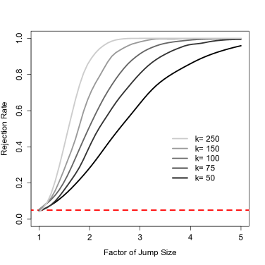
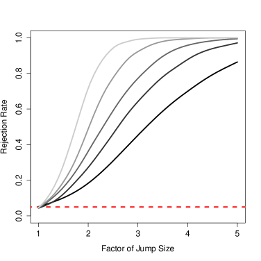
Figure 1: Rejection rate of the CP-Test for pure jump subordinator data (on the left-hand side) and a subordinator plus a drift and a Brownian motion (on the right-hand side). $\beta$ changes from $1$ to the factor of jump size.

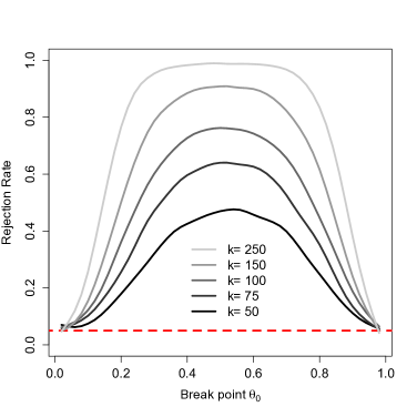
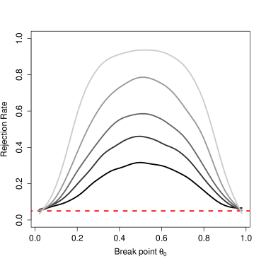
Figure 2: Rejection rate of the CP-Test for pure jump subordinator data (left panel) and a subordinator with a drift plus a Brownian motion (right panel) for different change point locations.

The next two graphics in Figure 2 show the rate of rejection of the CP-Test under alternatives involving one break point from $\beta=1$ to $\beta=2.5$ within the model in (5.1) for varying locations of the change point $\theta_{0}\in(0,1)$. Again, the left and right plots correspond to $b_{t}=\sigma_{t}\equiv 0$ and $\equiv 1$, respectively. Additionally to the general conclusions drawn from the results in Figure 1, we observe that break points can be detected best if $\theta_{0}=1/2$, and that the rejection rates are symmetric around that point.

Figure 3 shows the rejection rates of the KSCP-Test 1 and 2, evaluated at different points $z_{0}$, for one fixed alternative model involving a single change from $\beta=1$ to $\beta=2.5$ at the point $\theta_{0}=1/2$. The curves in the left plot are based on a pure jump process. We can see that the rejection rates are decreasing in $z_{0}$, explainable by the fact that there are only very few large jumps both for $\beta=1$ and for $\beta=2.5$. In the right plot, involving drift and volatility ($b_{t}=\sigma_{t}\equiv 1$), we observe a maximal value of the rejection rates that is increasing in the number of trading days, $k_{n}$. For values of $z_{0}$ smaller than this maximum, the contribution of the Brownian component (an independent normally distributed term with variance $\Delta_{n}$ within each increment $\Delta_{j}^{n}X$) predominates the jumps of that size and results in a decrease of the rejection rate.

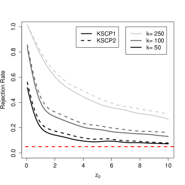
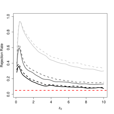
Figure 3: Rejection rates of the KSCP-Test 1 and 2 for different $z_{0}$. Left panel: pure jump subordinator, right panel: subordinator with a drift plus Brownian motion.

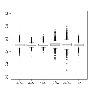
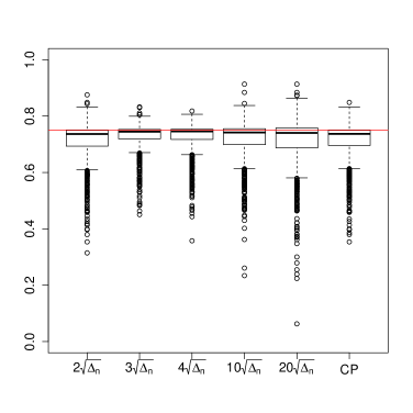
Figure 4: Box plots for the estimators $\tilde{\theta}_{n}^{(z_{0})}$ and $\hat{\theta}_{n}^{(\varepsilon)}$ based on a subordinator with a drift plus Brownian motion and a change from $\beta=1$ to $\beta=4$ at $\theta_{0}=0.5$ (left panel) and $\theta_{0}=0.75$ (right panel). The first five box plots in each panel correspond to five different choices of $z_{0}$.

Finally, in Figure 4, we depict box plots for the estimators $\tilde{\theta}_{n}^{\scriptscriptstyle(z_{0})}$ and $\hat{\theta}_{n}^{\scriptscriptstyle(\varepsilon)}$ of the change point for certain values of $z_{0}$ and for $M$ as specified in the case of Tables 1 and 2. The results are based on two models, involving a change in $\beta$ from $1$ to $4$ at time point $\theta_{0}=0.5$ (left panel) and $\theta_{0}=0.75$ (right panel) for $k_{n}=250$ and $\Delta_{n}^{-1}=90$, and with $b_{t}=\sigma_{t}\equiv 1$. We observe a reasonable approximation of the true value (indicated by the red line) with more accurate approximations for $\theta_{0}=0.5$. For $\theta_{0}=0.75$, the distribution of the estimator is skewed, giving more weight to the left tail directing to $\theta_{0}=0.5$. This might be explained by the fact that the distribution of the argmax absolute value of a tight-down stochastic process indexed by $\theta\in[0,1]$ gives very small weight to the boundaries of the unit interval. Moreover, as for the results presented in the right plot of Figure 3, the plots in Figure 4 reveal that the estimator $\tilde{\theta}_{n}^{\scriptscriptstyle(z_{0})}$ behaves best for an intermediate choice of $z_{0}$. Results for $b_{t}=\sigma_{t}\equiv 0$ are not depicted for the sake of brevity, since they do not transfer any additional insight.

6 Appendix

6.1 Proof of Lemma 2.2

Let $\varepsilon<(\delta/6\wedge 1)$ and pick a smooth cut-off function $c_{\varepsilon}:\mathbb{R}\to\mathbb{R}$ satisfying

$$1_{[-\varepsilon/2,\varepsilon/2]}(u)\leq c_{\varepsilon}(u)\leq 1_{[-\varepsilon,\varepsilon]}(u).$$

We also define the function $\bar{c}_{\varepsilon}$ via $\bar{c}_{\varepsilon}(u)=1-{c_{\varepsilon}}(u)$. We use $\bar{c}_{\epsilon}$ to define the “large” jumps of the process, that means, there exist independent processes $X^{\varepsilon}$ and $\widetilde{X}^{\varepsilon}$ such that $X=_{d}X^{\varepsilon}+\widetilde{X}^{\varepsilon}$ where $\widetilde{X}^{\varepsilon}$ is a compound Poisson process with intensity $\lambda_{\varepsilon}=\int\bar{c}_{\varepsilon}(u)\nu(du)$ and jump distribution $\rho_{\varepsilon}(du)=\bar{c}_{\varepsilon}(u)\nu(du)/\lambda_{\varepsilon}$. See e.g. Figueroa-Lopez and Houdre (2009). Accordingly, $X^{\varepsilon}$ is an Itō semimartingale with characteristics $(b^{\varepsilon}_{s},\sigma^{2}_{s},c_{\varepsilon}(u)\nu(du))$, where we set $b_{s}^{\epsilon}=b_{s}-\int 1_{\{|u|>1\}}u\bar{c}_{\varepsilon}(u)\nu(du)$.

Since our result is a distributional one only, it is possible to work with this particular representation of $X$ in the following. Call $N_{t}^{\varepsilon}$ the number of jumps of $\widetilde{X}^{\varepsilon}$ up to time $t$. Define $f(x)=1_{\{x\geq z\}}$. Using the law of total expectation we have

$$\mathbb{E}[f(X_{t})]=\sum_{k=0}^{\infty}e^{-\lambda_{\varepsilon}t}\frac{(\lambda_{\varepsilon}t)^{k}}{k!}\mathbb{E}[f(X_{t})|N_{t}^{\varepsilon}=k]\\ =e^{-\lambda_{\varepsilon}t}\mathbb{E}[f(X^{\varepsilon}_{t})]+e^{-\lambda_{\varepsilon}t}\lambda_{\varepsilon}t\mathbb{E}[f(X^{\varepsilon}_{t}+\xi_{1})]\\ +\sum_{k=2}^{\infty}e^{-\lambda_{\varepsilon}t}\frac{(\lambda_{\varepsilon}t)^{k}}{k!}\mathbb{E}\Big{[}f\Big{(}X^{\varepsilon}_{t}+\sum_{\ell=1}^{k}\xi_{\ell}\Big{)}\Big{]},$$ (6.1)

where the random variables $\xi_{\ell}$ are i.i.d. with distribution $\rho_{\varepsilon}$.

For the first summand on the right of the last display, i.e. the case of no large jumps, we discuss drift, volatility and small jumps separately. For that purpose, we write $X^{\varepsilon}_{t}=B^{\varepsilon}_{t}+Q_{t}+Y_{t}^{\varepsilon}$ where $B^{\varepsilon}_{t}=\int_{0}^{t}b_{s}^{\epsilon}ds$, $Q_{t}=\int_{0}^{t}\sigma_{s}dW_{s}$ and where $Y_{t}^{\varepsilon}$ is a pure jump Lévy martingale with jump measure $c_{\varepsilon}(u)\nu(du)$. By the triangle inequality

$$e^{-\lambda_{\varepsilon}t}\mathbb{E}[f(X^{\varepsilon}_{t})]\leq P(X^{\varepsilon}_{t}\geq\delta)\leq P(B^{\varepsilon}_{t}\geq\delta/3)+P(C_{t}\geq\delta/3)+P(Y^{\varepsilon}_{t}\geq\delta/3).$$

Let us show that the right-hand side of this display can be bounded by $Kt^{2}$ for all $0<t<t_{0}$, with constants $K=K(\delta)$ and $t_{0}=t_{0}(\delta)$. Regarding the summand $P(Y^{\varepsilon}_{t}\geq\delta/3)$, we can use equation (3.3) in Figueroa-Lopez and Houdre (2009) applied to a pure jump Lévy process. Following their result, $\varepsilon<\delta/6$ ensures the existence of $K$ and $t_{0}$, both depending on $\delta$ only, such that

$$\mathbb{P}(Y_{t}^{\varepsilon}\geq\delta/3)<Kt^{2}$$ (6.2)

for all $0<t<t_{0}$. Since $b$ and $\sigma$ are bounded, we further have $\mathbb{E}[|B^{\varepsilon}_{t}|^{r}]\leq Kt^{r}$ and $\mathbb{E}[|Q_{t}|^{r}]\leq Kt^{r/2}$ for an arbitrary integer $r$ and with $K$ depending on $\delta$ again. Markov’s inequality then yields bounds similar to (6.2) when applied to the processes involving drift, $B_{t}^{\varepsilon}$, and volatility, $C_{t}$.

Also, for the sum over $k$ on the right-hand side of (6.1), we have

$$e^{-\lambda_{\varepsilon}t}\sum_{k=2}^{\infty}\frac{(\lambda_{\varepsilon}t)^{k}}{k!}<Kt^{2}.$$

It therefore remains to focus on $\mathbb{E}[f(X^{\varepsilon}_{t}+\xi_{1})]$. As a consequence of Condition 2.1(d), and observing that the distribution of $\xi_{1}$ is $h(u)\bar{c}_{\varepsilon}(u)du/\lambda_{\varepsilon}$ with the Lévy density $h$, it follows that

$$g(x)=\mathbb{E}[f(x+\xi_{1})]=\mathbb{P}(x+\xi_{1}\geq z)$$

is twice continuously differentiable with bounded derivatives. Using independence of $X^{\varepsilon}$ and $\xi_{1}$, it is sufficient to discuss $\mathbb{E}[g(X_{t}^{\varepsilon})]$, for which we can use Itô formula now: for arbitrary $Y$ we have

$$g(Y_{t})=g(Y_{0})+\int_{0}^{t}g^{\prime}(Y_{s-})dY_{s}+\frac{1}{2}\int_{0}^{t}g^{\prime\prime}(Y_{s-})d[Y,Y]^{c}_{s}\\ +\sum_{0<s\leq t}\left(g(Y_{s})-g(Y_{s-})-g^{\prime}(Y_{s-})\Delta Y_{s})\right),$$ (6.3)

where $[Y,Y]^{c}_{s}$ denotes the quadratic variation and $\Delta Y_{s}$ is the jump size at time $s$. Plugging in $X^{\varepsilon}$ for $Y$ we discuss each of the four summands in (6.3) separately: first, $u\geq z$ implies $\bar{c}_{\varepsilon}(u)=1$ by definition of $\varepsilon$. Thus, with $X_{0}^{\varepsilon}=0$

$$g(X_{0}^{\varepsilon})=\mathbb{P}(\xi_{1}\geq z)=\frac{1}{\lambda_{\varepsilon}}\int 1_{\{u\geq z\}}h(u)\bar{c}_{\varepsilon}(u)du=\frac{1}{\lambda_{\varepsilon}}\int 1_{\{u\geq z\}}h(u)du=\frac{1}{\lambda_{\varepsilon}}\nu([z,\infty)).$$

Second, two of the three summands in $X^{\varepsilon}_{s}$ are martingales. Therefore

$$\left|\mathbb{E}\left[\int_{0}^{t}g^{\prime}(X^{\varepsilon}_{s-})dX^{\varepsilon}_{s}\right]\right|\leq\int_{0}^{t}\left|\mathbb{E}[g^{\prime}(X^{\varepsilon}_{s-})]b^{\varepsilon}_{s}\right|ds<Kt$$

due to boundedness of the first derivatives of $g$. We may proceed similarly for the third term in (6.3). Finally, conditioning on $X^{\varepsilon}_{s-}$ and using the definition of a compensator gives

$$\sum_{0<s\leq t}\mathbb{E}\left[g(X^{\varepsilon}_{s})-g(X^{\varepsilon}_{s-})-g^{\prime}(X^{\varepsilon}_{s-})\Delta X^{\varepsilon}_{s}\right]\\ =\int_{0}^{t}\int\mathbb{E}[g(X_{s-}^{\varepsilon}+u)-g(X_{s-}^{\varepsilon})-g^{\prime}(X_{s-}^{\varepsilon})u]c_{\varepsilon}(u)\nu(du)ds$$

for the final quantity. The Taylor formula proves that the inner integrand above may be bounded in absolute value by $Ku^{2}c_{\varepsilon}(u)$. Since $\nu$ is a Lévy measure, we obtain

$$\big{|}\mathbb{E}[g(X_{t}^{\varepsilon})]-\frac{1}{\lambda_{\varepsilon}}\nu([z,\infty))\big{|}<Kt.$$

From $|1-\exp(-\lambda_{\varepsilon}t)|<Kt$ for $0<t<t_{0}$ the conclusion follows. ∎

6.2 Proof of Theorem 2.4

Due to Theorem 1.6.1 in Van der Vaart and Wellner (1996), it suffices to prove weak convergence $\mathbb{G}_{n}\rightsquigarrow\mathbb{G}$ in $\ell^{\infty}(A_{k})$ for any fixed $k\in\mathbb{N}$.

To this end, we use Theorem 11.16 of Kosorok (2008). Note that $\mathbb{G}_{n}$ can be written as

$$\mathbb{G}_{n}(\theta,z)=\frac{1}{\sqrt{k_{n}}}\sum\limits_{j=1}^{\lfloor n\theta\rfloor}\{\mathtt{1}_{\{\Delta_{j}^{n}X\geq z\}}-\mathbb{P}(\Delta_{j}^{n}X\geq z)\}=\sum\limits_{j=1}^{n}\{f_{nj}(\omega;\theta,z)-\mathbb{E}f_{nj}(\cdot;\theta,z)\}$$

with the triangular array $\{f_{nj}(\omega;\theta,z)\mid n\geq 1;j=1,\ldots,n;(\theta,z)\in A_{k}\}$ consisting of the processes

$$f_{nj}(\theta,z):=f_{nj}(\omega;\theta,z):=\frac{1}{\sqrt{k_{n}}}\mathtt{1}_{\{j\leq\lfloor n\theta\rfloor\}}\mathtt{1}_{\{\Delta_{j}^{n}X(\omega)\geq z\}},$$

which are independent within rows since we assume a deterministic drift and volatility. By Theorem 11.16 in Kosorok (2008), the proof is complete if the following six conditions for $\{f_{nj}\}$ can be established:

1. $\{f_{nj}\}$ is almost measurable Suslin (AMS);

2. the $\{f_{nj}\}$ are manageable with envelopes $\{F_{nj}\mid n\in\mathbb{N},j=1,\ldots,n\}$ given through $F_{nj}:=k_{n}^{-1/2}\mathtt{1}_{\{\Delta_{j}^{n}X\geq k^{-1}\}}$, which are also independent within rows;

3. $H(\theta_{1},z_{1};\theta_{2},z_{2})=\lim\limits_{n\rightarrow\infty}\mathbb{E}\{\mathbb{G}_{n}(\theta_{1},z_{1})\mathbb{G}_{n}(\theta_{2},z_{2})\}$ for all $(\theta_{1},z_{1}),(\theta_{2},z_{2})\in A_{k}$;

4. $\limsup\limits_{n\rightarrow\infty}\sum\limits_{j=1}^{n}\mathbb{E}^{\ast}F_{nj}^{2}<\infty$;

5. $\lim\limits_{n\rightarrow\infty}\sum\limits_{j=1}^{n}\mathbb{E}^{\ast}F_{nj}^{2}\mathtt{1}_{\{F_{nj}>\varepsilon\}}=0$ for all $\varepsilon>0$;

6. $\rho(\theta_{1},z_{1};\theta_{2},z_{2})=\lim\limits_{n\rightarrow\infty}\rho_{n}(\theta_{1},z_{1};\theta_{2},z_{2})$ for every $(\theta_{1},z_{1}),(\theta_{2},z_{2})\in A_{k}$, where

   $$\rho_{n}(\theta_{1},z_{1};\theta_{2},z_{2}):=\bigg{\{}\sum\limits_{j=1}^{n}\mathbb{E}\left|f_{nj}(\cdot;\theta_{1},z_{1})-f_{nj}(\cdot;\theta_{2},z_{2})\right|^{2}\bigg{\}}^{\frac{1}{2}}.$$

   Moreover, $\rho_{n}(\theta_{1}^{(n)},z_{1}^{(n)};\theta_{2}^{(n)},z_{2}^{(n)})\rightarrow 0$ for all sequences $(\theta_{1}^{(n)},z_{1}^{(n)})_{n\in\mathbb{N}}$ and $(\theta_{2}^{(n)},z_{2}^{(n)})_{n\in\mathbb{N}}\subset A_{k}$ such that $\rho(\theta_{1}^{(n)},z_{1}^{(n)};\theta_{2}^{(n)},z_{2}^{(n)})\rightarrow 0$.

Proof of (1). By Lemma 11.15 in Kosorok (2008), the triangular array $\{f_{nj}\}$ is AMS provided it is separable, i.e., provided for every $n\in\mathbb{N}$, there exists a countable subset $S_{n}\subset A_{k}$, such that

$$\mathbb{P}^{\ast}\bigg{(}\sup\limits_{(\theta_{1},z_{1})\in A_{k}}\inf\limits_{(\theta_{2},z_{2})\in S_{n}}\sum\limits_{j=1}^{n}\{f_{nj}(\omega;\theta_{2},z_{2})-f_{nj}(\omega;\theta_{1},z_{1})\}^{2}>0\bigg{)}=0.$$

Define $S_{n}:=\mathbb{Q}^{2}\cap A_{k}$ for all $n\in\mathbb{N}$. Then, for every element $\omega$ of the underlying probability space and for every $(\theta_{1},z_{1})\in A_{k}$, there exists an $(\theta_{2},z_{2})\in S_{n}$ such that

$$\sum\limits_{j=1}^{n}\{f_{nj}(\omega;\theta_{2},z_{2})-f_{nj}(\omega;\theta_{1},z_{1})\}^{2}=0.$$

Proof of (2). The $\{F_{nj}\}$ are independent within rows since we assume deterministic characteristics of the underlying process. Therefore, according to Theorem 11.17 in Kosorok (2008), it suffices to prove that the triangular arrays

$$\{\tilde{f}_{nj}(\omega;z):=k_{n}^{-1/2}\mathtt{1}_{\{\Delta_{j}^{n}X\geq z\}}\mid n\in\mathbb{N};j=1,\ldots,n;z\in[k^{-1},\infty)\},$$

and

$$\{\tilde{g}_{nj}(\omega;\theta):=\mathtt{1}_{\{j\leq\lfloor n\theta\rfloor\}}\mid n\in\mathbb{N};j=1,\ldots,n;\theta\in[0,1]\}$$

are manageable with envelopes $\{\tilde{F}_{nj}(\omega):=k_{n}^{-1/2}\mathtt{1}_{\{\Delta_{j}^{n}X\geq k^{-1}\}}\mid n\in\mathbb{N};j=1,\ldots,n\}$ and $\{\tilde{G}_{nj}(\omega):\equiv 1\mid n\in\mathbb{N};j=1,\ldots,n\}$, respectively.

Concerning the first triangular array $\{\tilde{f}_{nj}\}$ define, for $\omega\in\Omega$ and $n\in\mathbb{N}$,

$$\mathcal{F}_{n\omega}:=\big{\{}(k_{n}^{-1/2}\mathtt{1}_{\{\Delta_{1}^{n}X(\omega)\geq z\}},\ldots,k_{n}^{-1/2}\mathtt{1}_{\{\Delta_{n}^{n}X(\omega)\geq z\}})\mid z\in[k^{-1},\infty)\big{\}}\subset\mathbb{R}^{n}.$$

For any $j_{1},j_{2}\in\{1,\ldots,n\}$, the projection $p_{j_{1},j_{2}}(\mathcal{F}_{n\omega})$ of $\mathcal{F}_{n\omega}$ onto the $j_{1}$-th and the $j_{2}$-th coordinate is an element of the set

$$\Big{\{}\{(0,0)\},\{(0,0),(k_{n}^{-1/2},0)\},\{(0,0),(0,k_{n}^{-1/2})\},\{(0,0),(k_{n}^{-1/2},k_{n}^{-1/2})\},\\ \{(0,0),(k_{n}^{-1/2},0),(k_{n}^{-1/2}k_{n}^{-1/2})\},\{(0,0),(0,k_{n}^{-1/2}),(k_{n}^{-1/2},k_{n}^{-1/2})\}\Big{\}}.$$

Hence, for every $t\in\mathbb{R}^{2}$, no proper coordinate projection of $\mathcal{F}_{n\omega}$ can surround $t$ in the sense of Definition 4.2 of Pollard (1990). Thus, $\mathcal{F}_{n\omega}$ is a subset of $\mathbb{R}^{n}$ of pseudodimension at most $1$ (Definition 4.3 in Pollard, 1990). Additionally, $\mathcal{F}_{n\omega}$ is a bounded set, whence Corollary 4.10 in Pollard (1990) yields the existence of constants $A$ and $W$, depending only on the pseudodimension, such that

$$D_{2}(x\|\alpha\odot\tilde{F}_{n}(\omega)\|_{2},\alpha\odot\mathcal{F}_{n\omega})\leq Ax^{-W}=:\lambda(x),$$

for all $0<x\leq 1$, for every rescaling vector $\alpha\in\mathbb{R}^{n}$ with non-negative entries and for all $\omega\in\Omega$ and $n\in\mathbb{N}$. Therein, $\|\cdot\|_{2}$ denotes the Euclidean distance, $D_{2}$ denotes the packing number with respect to the Euclidean distance and $\tilde{F}_{n}(\omega):=(\tilde{F}_{n1}(\omega),\ldots,\tilde{F}_{nn}(\omega))\in\mathbb{R}^{n}$ is the vector of envelopes. Since $\int_{0}^{1}\sqrt{\log\lambda(x)}dx<\infty$, the triangular array $\{\tilde{f}_{nj}\}$ is indeed manageable with envelopes $\{\tilde{F}_{nj}\}$.

Concerning the triangular array $\{\tilde{g}_{ni}\}$, we proceed similar and consider the set

$$\mathcal{G}_{n\omega}:=\{(\tilde{g}_{n1}(\omega;\theta),\ldots,\tilde{g}_{nn}(\omega;\theta))\mid\theta\in[0,1]\}\\ =\{(0,\ldots,0),(1,0,\ldots,0),(1,1,0,\ldots,0),\ldots,(1,\ldots,1)\}.$$

Then, for any $j_{1},j_{2}\in\{1,\ldots,n\}$, the projection $p_{j_{1},j_{2}}(\mathcal{G}_{n\omega})$ of $\mathcal{G}_{n\omega}$ onto the $j_{1}$-th and the $j_{2}$-th coordinate is either $\{(0,0),(1,0),(1,1)\}$ or $\{(0,0),(0,1),(1,1)\}$. Therefore, the same reasoning as above shows that $\mathcal{G}_{n\omega}$ is a set of pseudodimension at most one, whence the triangular array $\{\tilde{g}_{nj}\}$ is manageable with envelopes $\{\tilde{G}_{nj}\}$.

Proof of (3). For any $(\theta_{1},z_{1}),(\theta_{2},z_{2})\in A_{k}$, by independence of $\{f_{nj}\}$ within rows, we can write

$$\mathbb{E}\{\mathbb{G}_{n}(\theta_{1},z_{1})\mathbb{G}_{n}(\theta_{2},z_{2})\}$$

$$=\sum_{j=1}^{n}\mathbb{E}\big{[}\{f_{nj}(\omega;\theta_{1},z_{1})-\mathbb{E}f_{nj}(\cdot;\theta_{1},z_{1})\}\{f_{nj}(\omega;\theta_{2},z_{2})-\mathbb{E}f_{nj}(\cdot;\theta_{2},z_{2})\}\big{]}$$

$$=\frac{1}{k_{n}}\sum_{j=1}^{\lfloor n(\theta_{1}\wedge\theta_{2})\rfloor}\{\mathbb{P}(\Delta_{j}^{n}X\geq z_{1}\vee z_{2})-\mathbb{P}(\Delta_{j}^{n}X\geq z_{1})\mathbb{P}(\Delta_{j}^{n}X\geq z_{2})\}$$ (6.4)

By Remark 2.3 and the choice $K=K(k^{-1})$ and $t_{0}=t_{0}(k^{-1})>0$, we have

$$\mathbb{P}(\Delta_{j}^{n}X\geq z)=\Delta_{n}\nu([z,\infty))+O(\Delta_{n}^{2}),\quad n\to\infty$$ (6.5)

for all $z\geq k^{-1}$ and all $j=1,\ldots,n$, whence the right-hand side of equation (6.2) can be written as

$$\frac{\lfloor n(\theta_{1}\wedge\theta_{2})\rfloor}{n}\{\nu([z_{1}\vee z_{2},\infty))+O(\Delta_{n})\}=H(\theta_{1},z_{1};\theta_{2},z_{2})+o(1),\quad n\to\infty.$$

Proof of (4). Again from Remark 2.3, we have

$$\sum\limits_{j=1}^{n}\mathbb{E}^{\ast}F_{nj}^{2}=\frac{1}{n\Delta_{n}}\sum\limits_{j=1}^{n}\mathbb{P}(\Delta_{j}^{n}X\geq k^{-1})=\nu([k^{-1},\infty))+O(\Delta_{n})\rightarrow\nu([k^{-1},\infty))<\infty$$

as $n\to\infty$.

Proof of (5). For $\varepsilon>0$ define $N:=\min\{n\in\mathbb{N}\mid k_{m}^{-1/2}\leq\varepsilon\text{ for all }m\geq n\}$. Choose $K=K(k^{-1})$ and $t_{0}=t_{0}(k^{-1})$ as in Lemma 2.2. Then, for any sufficiently large $n$ such that $\Delta_{n}<t_{0}$, we have

$$\sum\limits_{j=1}^{n}\mathbb{E}^{\ast}F_{nj}^{2}\mathtt{1}_{\{F_{nj}>\varepsilon\}}\leq\sum\limits_{j=1}^{N}\mathbb{E}^{\ast}F_{nj}^{2}=\frac{1}{n\Delta_{n}}\sum\limits_{j=1}^{N}\mathbb{P}(\Delta_{j}^{n}X\geq k^{-1})\\ \leq\frac{N}{n}\{\nu([k^{-1},\infty))+K\Delta_{n}\}\to 0,\qquad n\to\infty.$$

Proof of (6). For $(\theta_{1},z_{1}),(\theta_{2},z_{2})\in A_{k}$, we can write

$$\rho_{n}^{2}( \theta_{1},z_{1};\theta_{2},z_{2})$$

$$=\sum\limits_{j=1}^{n}\mathbb{E}\left|f_{nj}(\cdot;\theta_{1},z_{1})-f_{nj}(\cdot;\theta_{2},z_{2})\right|^{2}$$

$$=\frac{1}{n\Delta_{n}}\bigg{\{}\sum_{j=1}^{\lfloor n(\theta_{1}\wedge\theta_{2})\rfloor}(\mathbb{P}(\Delta_{j}^{n}X\geq z_{1}\wedge z_{2})-\mathbb{P}(\Delta_{j}^{n}X\geq z_{1}\vee z_{2}))$$

$$\hskip 182.09746pt+\sum\limits_{j=\lfloor n(\theta_{1}\wedge\theta_{2})\rfloor+1}^{\lfloor n(\theta_{1}\vee\theta_{2})\rfloor}\mathbb{P}(\Delta_{j}^{n}X\geq z_{I(\theta_{1},\theta_{2})})\bigg{\}}$$

$$=\big{\{}(\theta_{1}\wedge\theta_{2})+O(n^{-1})\big{\}}\times\big{\{}\nu([z_{1}\wedge z_{2},z_{1}\vee z_{2}))+O(\Delta_{n})\big{\}}$$

$$\hskip 113.81102pt+\big{\{}\left|\theta_{1}-\theta_{2}\right|+O(n^{-1})\big{\}}\times\big{\{}\nu([z_{I(\theta_{1},\theta_{2})},\infty))+O(\Delta_{n})\big{\}}$$

as $n\to\infty$, where the $O$-terms are uniform in $(\theta_{1},z_{1}),(\theta_{2},z_{2})\in A_{k}$ for the same reason as in equation (6.5). Thus $\rho_{n}^{2}$ converges even uniformly on each $A_{k}\times A_{k}$ to $\rho^{2}$. Consequently, for any sequences $(\theta_{1}^{\scriptscriptstyle(n)},z_{1}^{\scriptscriptstyle(n)})_{n\in\mathbb{N}},(\theta_{2}^{\scriptscriptstyle(n)},z_{2}^{\scriptscriptstyle(n)})_{n\in\mathbb{N}}\subset A_{k}$ such that $\rho(\theta_{1}^{\scriptscriptstyle(n)},z_{1}^{\scriptscriptstyle(n)};\theta_{2}^{\scriptscriptstyle(n)},z_{2}^{\scriptscriptstyle(n)})\rightarrow 0$, it follows $\rho_{n}(\theta_{1}^{\scriptscriptstyle(n)},z_{1}^{\scriptscriptstyle(n)};\theta_{2}^{\scriptscriptstyle(n)},z_{2}^{\scriptscriptstyle(n)})\rightarrow 0$.

Finally, $\rho$ is a semimetric: applying first the triangle inequality in $\mathbb{R}^{n}$ and then the Minkowski inequality, one sees that each $\rho_{n}$ satisfies the triangle inequality. Thus the triangle inequality also holds for $\rho$. ∎

6.3 Proof of Corollary 2.5

For $k\in\mathbb{N}$, choose $K=K(k^{-1})$ and $t_{0}=t_{0}(k^{-1})$ as in Lemma 2.2. Then, for any $(\theta,z)\in A_{k}$ and for sufficiently large $n$, we have

$$|\mathbb{G}_{n} (\theta,z)-\tilde{\mathbb{G}}_{n}(\theta,z)|=\sqrt{k_{n}}|\mathbb{E}U_{n}(\theta,z)-\theta\nu([z,\infty))|$$

$$\leq\sqrt{k_{n}}\left|\frac{1}{n}\sum\limits_{j=1}^{\lfloor n\theta\rfloor}\{\Delta_{n}^{-1}\mathbb{P}(\Delta_{j}^{n}X\geq z)-\nu([z,\infty))\}\right|+\sqrt{k_{n}}\nu([z,\infty))\left|\frac{\lfloor n\theta\rfloor}{n}-\theta\right|$$

$${\leq}K\sqrt{k_{n}}\Delta_{n}+\nu([k^{-1},\infty))\sqrt{\frac{\Delta_{n}}{n}}\rightarrow 0.$$

because of equation (6.5). Since the convergence is uniform in $(\theta,z)\in A_{k}$, we obtain that $d(\mathbb{G}_{n},\tilde{\mathbb{G}}_{n})\to 0$ in probability. Lemma 1.10.2(i) in Van der Vaart and Wellner (1996) yields the assertion. ∎

6.4 Proof of Theorem 2.6

We are going to use the extended continuous mapping theorem (Theorem 1.11.1 in Van der Vaart and Wellner, 1996). For $n\in\mathbb{N}_{0}$, define $g_{n}\colon\mathcal{B}_{\infty}(\mathbb{A})\rightarrow\mathcal{B}_{\infty}(\mathbb{A})$ through

$$g_{n}(f) (\theta,z)=f(\theta,z)-\frac{\lfloor n\theta\rfloor}{n}f(1,z),\quad\text{ for }n\in\mathbb{N}$$

and

$$g_{0}(f) (\theta,z)=f(\theta,z)-\theta f(1,z)\}.$$

Note that $g_{n}$ is Lipschitz continuous for any $n\in\mathbb{N}_{0}$.

Obviously, $\mathbb{T}_{n}=g_{n}(\mathbb{G}_{n})+\mathbb{E}\mathbb{T}_{n}$ for each $n\in\mathbb{N}$ and $\mathbb{T}=g_{0}(\mathbb{G})$. We have

$$\mathbb{E}\mathbb{T}_{n}(\theta,z)=\sqrt{k_{n}}\lambda_{n}(\theta)\left\{\frac{n}{\lfloor n\theta\rfloor}\mathbb{E}U_{n}(\theta,z)-\frac{n}{n-\lfloor n\theta\rfloor}[\mathbb{E}U_{n}(1,z)-\mathbb{E}U_{n}(\theta,z)]\right\}$$

and the proof of Corollary 2.5 shows that $\mathbb{E}\mathbb{T}_{n}$ converges to $0$ in $\mathcal{B}_{\infty}(\mathbb{A})$. Thus, by Slutsky’s theorem (Van der Vaart and Wellner, 1996, Example 1.4.7), it suffices to verify $g_{n}(\mathbb{G}_{n})\rightsquigarrow g_{0}(\mathbb{G})$.

Due to Theorem 1.11.1 in Van der Vaart and Wellner (1996) (note that $\mathbb{G}$ is separable as it is tight; see Lemma 1.3.2 in the last-named reference) this weak convergence is valid, if we can show that, for any sequence $(f_{n})_{n\in\mathbb{N}}\subset\mathcal{B}_{\infty}(\mathbb{A})$ with $f_{n}\rightarrow f_{0}$ for some $f_{0}\in\mathcal{B}_{\infty}(\mathbb{A})$, we have

$$g_{n}(f_{n})\rightarrow g_{0}(f_{0}).$$

Let $(f_{n})_{n\in\mathbb{N}}$ be such a sequence with limit point $f_{0}$. Convergence in $(\mathcal{B}_{\infty}(\mathbb{A}),d)$ is equivalent to uniform convergence on each $A_{k}$ with $k\in\mathbb{N}$. The latter is true since

$$\|g_{n}(f_{n})-g_{0}(f_{0})\|_{A_{k}} =\|f_{n}(\theta,z)-(\lfloor n\theta\rfloor/n)f_{n}(1,z)-f_{0}(\theta,z)+\theta f_{0}(1,z)\|_{A_{k}}$$

$$\leq n^{-1}\|f_{0}\|_{A_{k}}+2\|f_{n}-f_{0}\|_{A_{k}}.$$

Obviously, $\mathbb{T}$ is a tight, mean-zero Gaussian process. Moreover, from Theorem 2.4,

$$\operatorname{Cov}\{\mathbb{T}(\theta_{1},z_{1}),\mathbb{T}(\theta_{2},z_{2})\} =H(\theta_{1},z_{1};\theta_{2},z_{2})-\theta_{1}H(1,z_{1};\theta_{2},z_{2})$$

$$\hskip 85.35826pt-\theta_{2}H(\theta_{1},z_{1};1,z_{2})+\theta_{1}\theta_{2}H(1,z_{1};1,z_{2})$$

$$=\{(\theta_{1}\wedge\theta_{2})-\theta_{1}\theta_{2}\}\nu([z_{1}\vee z_{2},\infty))$$

for any $(\theta_{1},z_{1}),(\theta_{2},z_{2})\in\mathbb{A}$. ∎

6.5 Proof of Proposition 2.8

Because of Corollary 2.5 (and the continuous mapping theorem) $U_{1:n}(z_{0})=U_{n}(1,z_{0})$ converges to $\nu([z_{0},\infty))>0$ in probability. Therefore, it follows easily that the random variable $\{U_{n}(1,z_{0})\}^{-1/2}\mathtt{1}_{\{U_{n}(1,z_{0})>0\}}$ converges to $\{\nu([z_{0},\infty))\}^{-1/2}$ in probability. Hence, by Slutsky’s theorem (Van der Vaart and Wellner, 1996, Example 1.4.7) we obtain

$$V_{n}^{(z_{0})}(\theta)\rightsquigarrow\frac{1}{\sqrt{\nu([z_{0},\infty))}}\mathbb{T}(\theta,z_{0}).$$

By Theorem 2.6 the process on the right-hand side of this display is a tight mean zero Gaussian with covariance function $k(\theta_{1},\theta_{2})=\theta_{1}\wedge\theta_{2}-\theta_{1}\theta_{2}$. Thus, the law of that process is the law of a standard Brownian bridge on $\ell^{\infty}([0,1])$. ∎

6.6 Proof of Theorem 3.3

Due to Lemma 6.2 below it suffices to prove conditional weak convergence on $\ell^{\infty}(A_{k})$ for any fixed $k\in\mathbb{N}$. Recall the triangular array $\{f_{nj}(\omega;\theta,z)\mid n\geq 1;j=1,\ldots,n;(\theta,z)\in A_{k}\}$ consisting of the processes

$$f_{nj}(\omega;\theta,z):=k_{n}^{-1/2}\mathtt{1}_{\{j\leq\lfloor n\theta\rfloor\}}\mathtt{1}_{\{\Delta_{j}^{n}X\geq z\}}.$$

Set $\mu_{nj}(\theta,z):=\mathbb{E}f_{nj}(\cdot;\theta,z)=k_{n}^{-1/2}\mathtt{1}_{\{j\leq\lfloor n\theta\rfloor\}}\mathbb{P}(\Delta_{j}^{n}X\geq z)$ and let

$$\hat{\mu}_{nj}(\theta,z):=\hat{\mu}_{nj}(\omega;\theta,z):=k_{n}^{-1/2}\mathtt{1}_{\{j\leq\lfloor n\theta\rfloor\}}\eta_{n}(z)$$

be an estimator for $\mu_{nj}(\theta,z)$. Then, $\hat{\mathbb{G}}_{n}$ can be written as

$$\hat{\mathbb{G}}_{n}(\theta,z)=\hat{\mathbb{G}}_{n}(\omega;\theta,z)=\sum\limits_{j=1}^{n}\xi_{j}\{f_{nj}(\omega;\theta,z)-\hat{\mu}_{nj}(\omega;\theta,z)\}.$$

Due to Theorem 3 in Kosorok (2003) the proof is complete, if we show the following properties for the triangular array $\{\hat{\mu}_{nj}(\omega;\theta,z)\mid n\geq 1;j=1,\ldots,n;(\theta,z)\in A_{k}\}$:

1. $\{\hat{\mu}_{nj}\}$ is almost measurable Suslin.

2. $\sup\limits_{(\theta,z)\in A_{k}}\sum\limits_{j=1}^{n}\{\hat{\mu}_{nj}(\omega;\theta,z)-\mu_{nj}(\theta,z)\}^{2}\stackrel{{\scriptstyle\scriptscriptstyle\mathbb{P}^{*}}}{{\rightarrow}}0.$

3. The triangular array $\{\hat{\mu}_{nj}\}$ is manageable with envelopes $\{\hat{F}_{nj}\}$ given through $\hat{F}_{nj}(\omega):=k_{n}^{-1/2}n^{-1}\sum_{i=1}^{n}\mathtt{1}_{\{\Delta_{i}^{n}X\geq k^{-1}\}}$.

4. There exists a constant $M<\infty$ such that $M\vee\sum\limits_{j=1}^{n}\hat{F}_{nj}^{2}\stackrel{{\scriptstyle\scriptscriptstyle\mathbb{P}^{*}}}{{\rightarrow}}M$.

Proof of (i). As in the proof of (1) in Theorem 2.4, it suffices to verify that the triangular array $\{\hat{\mu}_{nj}\}$ is separable. This can be seen by taking $S_{n}:=A_{k}\cap\mathbb{Q}^{2}$ again.

Proof of (ii). We have

$$\sup\limits_{(\theta,z)\in A_{k}}\sum_{j=1}^{n}\{\hat{\mu} {}_{nj}(\omega;\theta,z)-\mu_{nj}(\theta,z)\}^{2}$$

$$=\sup\limits_{z\geq 1/k}n^{-3}\Delta_{n}^{-1}\sum\limits_{j=1}^{n}\bigg{[}\sum\limits_{i=1}^{n}\{\mathtt{1}_{\{\Delta_{i}^{n}X\geq z\}}-\mathbb{P}(\Delta_{j}^{n}X\geq z)\}\bigg{]}^{2}$$

$$=n^{-1}\sup\limits_{z\geq 1/k}\{\mathbb{G}_{n}(1,z)\}^{2}+O_{\mathbb{P}}(\Delta_{n}^{2}),$$

where the final approximation error is a consequence of equation (6.5) in the proof of Theorem 2.4. The last quantity in the above display converges to $0$ in probability by Theorem 2.4.

Proof of (iii). In the proof of Theorem 2.4 we have already shown that the triangular array

$$\{\tilde{g}_{nj}(\theta):=\tilde{g}_{nj}(\omega;\theta):=\mathtt{1}_{\{j\leq\lfloor n\theta\rfloor\}}\mid n\in\mathbb{N};j=1,\ldots,n;\theta\in[0,1]\}$$

is manageable with envelopes $\{\tilde{G}_{nj}(\omega)\stackrel{{\scriptstyle\mathrm{def}}}{{\equiv}}1\mid n\in\mathbb{N};j=1,\ldots,n\}$. Therefore, due to Theorem 11.17 in Kosorok (2008), it suffices to prove that the triangular array

$$\left\{\tilde{h}_{nj}(\omega;z):=\frac{1}{n\sqrt{k_{n}}}\sum\limits_{i=1}^{n}\mathtt{1}_{\{\Delta_{i}^{n}X\geq z\}}\mid n\in\mathbb{N};j=1,\ldots,n;z\in[k^{-1},\infty)\right\}$$

is manageable with envelopes $\{\hat{F}_{nj}(\omega)\mid n\in\mathbb{N};j=1,\ldots,n\}$. But $\tilde{h}_{nj}(\omega;z)$ does not depend on $j$ at all, such that every projection of $\mathcal{H}_{n\omega}:=\{(\tilde{h}_{n1}(\omega;z),\ldots,\tilde{h}_{nn}(\omega;z))\mid z\geq k^{-1}\}$ onto two coordinates lies in the straight line $\{(x,y)\in\mathbb{R}^{2}\mid x=y\}$. Consequently, the set $\mathcal{H}_{n\omega}$ has a pseudodimension of at most $1$ (Definition 4.3 in Pollard, 1990) and is bounded. Hence, the same arguments as in the proof of Theorem 2.4 show the desired manageability.

Proof of (iv). A straight forward calculation yields

$$\mathbb{E}\left\{\sum\limits_{j=1}^{n}\hat{F}_{nj}^{2}\right\}=n^{-2}\Delta_{n}^{-1}\sum\limits_{i_{1}=1}^{n}\sum\limits_{i_{2}=1}^{n}\mathbb{E}\left\{\mathtt{1}_{\{\Delta_{i_{1}}^{n}X\geq k^{-1}\}}\mathtt{1}_{\{\Delta_{i_{2}}^{n}X\geq k^{-1}\}}\right\}=O(\Delta_{n}).$$

Here we used equation (6.5) again and the fact, that the increments of $X$ are independent since we assume deterministic characteristics. Thus $\sum\limits_{j=1}^{n}\hat{F}_{nj}^{2}$ is $o_{\mathbb{P}}(1)$. ∎

6.7 Proof of Theorem 3.4

Again by Lemma 6.2 it suffices to prove the convergence in the spaces $\ell^{\infty}(A_{k})$. Let therefore $k\in\mathbb{N}$ be fixed for the rest of the proof.

By definition, $\hat{\mathbb{T}}_{n}=g_{n}(\hat{\mathbb{G}}_{n})$ in $\ell^{\infty}(A_{k})$, with $g_{n}$ defined in the proof of Theorem 2.6. Now, $(\ell^{\infty}(A_{k}),\|\cdot\|_{A_{k}})$ is a Banach space and the mapping $g_{0}\colon\ell^{\infty}(A_{k})\rightarrow\ell^{\infty}(A_{k})$ defined in the proof of Theorem 2.6 is Lipschitz continuous. Hence, Proposition 10.7(i) in Kosorok (2008) yields the convergence

$$g_{0}(\hat{\mathbb{G}}_{n}){\,{\rightsquigarrow_{\xi}}\ }g_{0}(\mathbb{G})=\mathbb{T}$$

in $\ell^{\infty}(A_{k})$. Furthermore, due to the definition of the mappings $g_{n},g_{0}$ and the definition of the process $\hat{\mathbb{G}}_{n}$ we obtain that

$$\|g_{n}(\hat{\mathbb{G}}_{n})-g_{0}(\hat{\mathbb{G}}_{n})\|_{A_{k}}\leq\frac{1}{n}\sup\limits_{z\geq\frac{1}{k}}|\hat{\mathbb{G}}_{n}(1,z)|$$

By Theorem 3.3, the right-hand side converges to $0$ in probability. Another application of Lemma 6.1 shows that $\mathbb{T}_{n}=g_{n}(\hat{\mathbb{G}}_{n}){\,{\rightsquigarrow_{\xi}}\ }g_{0}(\mathbb{G})=\mathbb{T}$ as asserted. ∎

6.8 Proof of Proposition 4.1

The assertion that $\lim_{n\rightarrow\infty}\mathbb{P}(V_{n}^{(z_{0})}\geq q^{K}_{1-\alpha})=\alpha$ under $\textbf{H}_{0}$ is a simple consequence of Proposition 2.8 and the fact that the KS-distribution has a continuous cumulative distribution function.

With respect to the assertion regarding $W_{n}^{\scriptscriptstyle(z_{0})}$ note that, under $\textbf{H}_{0}$, Proposition 6.3 and the continuous mapping theorem imply that, for any fixed $B\in\mathbb{N}$,

$$(W_{n}^{(z_{0})},\hat{W}_{n,\xi^{(1)}}^{(z_{0})},\ldots,\hat{W}_{n,\xi^{(B)}}^{(z_{0})})\rightsquigarrow(W^{(z_{0})},W^{(z_{0}),(1)},\ldots,W^{(z_{0}),(B)})$$

in $\mathbb{R}^{B+1}$, where $W^{(z_{0})}:=\sup_{\theta\in[0,1]}|\mathbb{T}(\theta,z_{0})|$ with the limit process $\mathbb{T}$ of Theorem 2.6 and where $W^{(z_{0}),(1)},\ldots,W^{(z_{0}),(B)}$ are independent copies of $W^{(z_{0})}$. According to the corollary to Proposition 3 in Lifshits (1984), $W^{(z_{0})}$ has a continuous c.d.f. under $\textbf{H}_{0}$. Thus, Proposition F.1 in the supplement to Bücher and Kojadinovic (2014) implies that

$$\lim\limits_{B\rightarrow\infty}\lim\limits_{n\rightarrow\infty}\mathbb{P}\{W_{n}^{(z_{0})}\geq\hat{q}_{1-\alpha}^{(B)}(W_{n}^{(z_{0})})\}=\alpha$$

for all $\alpha\in(0,1)$, as asserted. Observing that, under $\textbf{H}_{0}$ and for $\varepsilon>0$ with $\nu([\varepsilon,\infty))>0$, the distribution of $T^{(\varepsilon)}$ has a continuous c.d.f., essentially the same reasoning also implies that

$$\lim_{B\rightarrow\infty}\lim_{n\rightarrow\infty}\mathbb{P}\{T_{n}^{(\varepsilon)}\geq\hat{q}_{1-\alpha}^{(B)}(T_{n}^{(\varepsilon)})\}=\alpha$$

for all $\alpha\in(0,1)$. ∎

6.9 Proof of Proposition 4.2

In order to prove consistency of the CP-Test, choose $\varepsilon>0$ as in Proposition 6.4 such that $\lim_{n\rightarrow\infty}\mathbb{P}(T_{n}^{\scriptscriptstyle(\varepsilon)}\geq K)=1$ for any $K>0$. By Proposition 6.5, for given $\delta>0$ and fixed $B\in\mathbb{N}$, we may choose $K_{0}>0$ such that

$$\sup\limits_{n\in\mathbb{N}}\mathbb{P}\Big{(}\max\limits_{b=1,\ldots,B}\hat{T}_{n,\xi^{(b)}}^{(\varepsilon)}>K_{0}\Big{)}\leq\frac{\delta}{2}.$$

For this $K_{0}$, we can now take $N\in\mathbb{N}$ such that

$$\mathbb{P}(T_{n}^{(\varepsilon)}\geq K_{0})\geq 1-\frac{\delta}{2}$$

holds for all $n\geq N$. Then, for any $n\geq N$,

$$1-\delta \leq\mathbb{P}(T_{n}^{(\varepsilon)}\geq K_{0})-\mathbb{P}\Big{(}\max\limits_{b=1,\ldots,B}\hat{T}_{n,\xi^{(b)}}^{(\varepsilon)}>K_{0}\Big{)}$$

$$\leq\mathbb{P}\Big{(}T_{n}^{(\varepsilon)}\geq K_{0},\max\limits_{b=1,\ldots,B}\hat{T}_{n,\xi^{(b)}}^{(\varepsilon)}\leq K_{0}\Big{)}$$

$$\leq\mathbb{P}\big{\{}T_{n}^{(\varepsilon)}\geq\hat{q}_{1-\alpha}^{(B)}(T_{n}^{(\varepsilon)})\big{\}}.$$

This proves the assertion for the CP-Test, and the claim for KSCP-Test2 follows along the same lines. The assertion for KSCP-Test1 is a direct consequence of Proposition 6.4. ∎

6.10 Proof of Proposition 4.3

Let $X^{\scriptscriptstyle(1)}(n)$ and $X^{\scriptscriptstyle(2)}(n)$ denote two independent Itō semimartingales with characteristics $(b^{\scriptscriptstyle(n)}_{t},\sigma^{\scriptscriptstyle(n)}_{t},\nu_{1})$ and $(b^{\scriptscriptstyle(n)}_{t},\sigma^{\scriptscriptstyle(n)}_{t},\nu_{2})$, respectively. For $n\in\mathbb{N}$ and $j=0,\dots,n$, set $Y_{j}(n)=X_{j\Delta_{n}}^{\scriptscriptstyle(1)}(n)$ and $Z_{j}(n)=X_{j\Delta_{n}}^{\scriptscriptstyle(2)}(n)$. Let $U_{n}^{\scriptscriptstyle(1)}$ and $U_{n}^{\scriptscriptstyle(2)}$ denote the quantity defined in (2.1), based on the observations $Y_{j}(n)$ and $Z_{j}(n)$, respectively, instead on $X_{j\Delta_{n}}$. Moreover, define a random element $S_{n}$ with values in $\mathcal{B}_{\infty}(\mathbb{A})$ through

$$S_{n}(\theta,z):=\frac{n-\lfloor n\theta\rfloor}{n}U_{n}^{(1)}(\theta,z)-\frac{\lfloor n\theta\rfloor}{n}\{U_{n}^{(1)}(\theta_{0},z)-U_{n}^{(1)}(\theta,z)\}\\ -\frac{\lfloor n\theta\rfloor}{n}\{U_{n}^{(2)}(1,z)-U_{n}^{(2)}(\theta_{0},z)\},$$

for $(\theta,z)\in\mathbb{A}$ with $\theta\leq\theta_{0}$, whereas for $(\theta,z)\in\mathbb{A}$ with $\theta\geq\theta_{0}$,

$$S_{n}(\theta,z):=\frac{n-\lfloor n\theta\rfloor}{n}U_{n}^{(1)}(\theta_{0},z)+\frac{n-\lfloor n\theta\rfloor}{n}\{U_{n}^{(2)}(\theta,z)-U_{n}^{(2)}(\theta_{0},z)\}\\ -\frac{\lfloor n\theta\rfloor}{n}\{U_{n}^{(2)}(1,z)-U_{n}^{(2)}(\theta,z)\}.$$

According to Theorem II.4.15 in Jacod and Shiryaev (2002), we have the distributional equality

$$\big{(}\Delta_{1}^{n}X(n),\ldots,\Delta_{\lfloor n\theta_{0}\rfloor}^{n}X(n),\Delta_{\lfloor n\theta_{0}\rfloor+1}^{n}X(n),\ldots,\Delta_{n}^{n}X(n)\big{)}\\ \stackrel{{\scriptstyle\mathcal{D}}}{{=}}\big{(}\Delta_{1}^{n}X^{(1)}(n),\ldots,\Delta_{\lfloor n\theta_{0}\rfloor}^{n}X^{(1)}(n),\Delta_{\lfloor n\theta_{0}\rfloor+1}^{n}X^{(2)}(n),\ldots,\Delta_{n}^{n}X^{(2)}(n)\big{)}.$$

Hence, for any $(\theta_{1},z_{1}),\ldots,(\theta_{p},z_{p})\in\mathbb{A}$ and $p\in\mathbb{N}$, we also have that

$$\big{(}k_{n}^{-1/2}\mathbb{T}_{n}(\theta_{1},z_{1}),\ldots,k_{n}^{-1/2}\mathbb{T}_{n}(\theta_{g},z_{g})\big{)}\stackrel{{\scriptstyle\mathcal{D}}}{{=}}\big{(}S_{n}(\theta_{1},z_{1}),\ldots,S_{n}(\theta_{g},z_{g})\big{)}.$$

By Theorem 1.6.1 in Van der Vaart and Wellner (1996), we have to show uniform convergence of $k_{n}^{\scriptscriptstyle-1/2}\mathbb{T}_{n}$ to $T$ on any $A_{k}$ with $k\in\mathbb{N}$, in probability. Now, from the previous display, and from the fact that the function $T$ is continuous in $(\theta,z)$ and that the functions $\mathbb{T}_{n}(\theta,z)$ depend only through $\lfloor n\theta\rfloor$ on $\theta$ and are left-continuous in $z$, we immediately get that

$$\sup\limits_{(\theta,z)\in A_{k}}\left|k_{n}^{-1/2}\mathbb{T}_{n}(\theta,z)-T(\theta,z)\right| =\sup\limits_{(\theta,z)\in A_{k}\cap\mathbb{Q}^{2}}\left|k_{n}^{-1/2}\mathbb{T}_{n}(\theta,z)-T(\theta,z)\right|$$

$$\stackrel{{\scriptstyle\mathcal{D}}}{{=}}\sup\limits_{(\theta,z)\in A_{k}\cap\mathbb{Q}^{2}}\left|S_{n}(\theta,z)-T(\theta,z)\right|$$

This expression is in fact $o_{\mathbb{P}}(1)$ as a consequence of Corollary 2.5 and the continuous mapping theorem. Note that the proofs of Lemma 2.2, Theorem 2.4 and Corollary 2.5 show that Corollary 2.5 is in fact applicable in this setup, because the characteristics $b^{\scriptscriptstyle(n)}_{t}$ and $\sigma^{\scriptscriptstyle(n)}_{t}$ have a uniform bound in $n\in\mathbb{N}$ and the resulting constants of Lemma 2.2 depend only on the bound of the characteristics and on $\delta$. ∎

6.11 Proof of Proposition 4.4

Under $\mathbf{H}_{1}$, choose $\varepsilon>0$ such that there exists a $z_{0}\geq\varepsilon$ with $\nu_{1}(z_{0})\neq\nu_{2}(z_{0})$. Then, according to Proposition 4.3 and the continuous mapping theorem, the random functions $\theta\mapsto\sup_{z\geq\varepsilon}|k_{n}^{\scriptscriptstyle-1/2}\mathbb{T}_{n}(\theta,z)|$ converge weakly in $\ell^{\infty}([0,1])$ to the continuous function $\theta\mapsto\sup_{z\geq\varepsilon}|T(\theta,z)|$, which has a unique maximum at $\theta_{0}$.

Similarly, under $\textbf{H}_{1}^{\scriptscriptstyle(z_{0})}$, the random functions $\theta\mapsto|k_{n}^{\scriptscriptstyle-1/2}\mathbb{T}_{n}(\theta,z_{0})|$ converge weakly in $\ell^{\infty}([0,1])$ to the continuous function $\theta\mapsto|T(\theta,z_{0})|$, which also has a unique maximum in $\theta_{0}$.

Thus, the asserted convergences follow from the argmax-continuous mapping theorem (Theorem 2.7 in Kim and Pollard, 1990). ∎

6.12 Additional auxiliary results

The following two auxiliary results are needed for validating the bootstrap procedures defined in Section 3. The first lemma is proved in Bücher (2011), Lemma A.1.

Lemma 6.1.

Consider two bootstrapped statistics $\hat{G}_{n}=\hat{G}_{n}(X_{1},\ldots,X_{n},\xi_{1},\ldots,\xi_{n})$ and $\hat{H}_{n}=\hat{H}_{n}(X_{1},\ldots,X_{n},\xi_{1},\ldots,\xi_{n})$ in a metric space $(\mathbb{D},d)$ with $d(\hat{G}_{n},\hat{H}_{n})\stackrel{{\scriptstyle\scriptscriptstyle\mathbb{P}^{*}}}{{\rightarrow}}0$. Then, for a tight Borel measurable process $G$ in $\mathbb{D}$, we have $\hat{G}_{n}{\,{\rightsquigarrow_{\xi}}\ }G$ if and only if $\hat{H}_{n}{\,{\rightsquigarrow_{\xi}}\ }G$.

For the second auxiliary lemma, let $T_{1}\subset T_{2}\subset\ldots$ be arbitrary sets and set $T:=\bigcup_{k=1}^{\infty}T_{k}$. Let $(\mathcal{B}_{\infty}(T),d)$ be defined as the complete metric space of all real-valued functions on $T$ that are bounded on each $T_{k}$, equipped with the metric

$$d(f_{1},f_{2})=\sum\limits_{k=1}^{\infty}2^{-k}(\|f_{1}-f_{2}\|_{T_{k}}\wedge 1),$$

where $\|\cdot\|_{T_{k}}$ denotes the sup-norm on $T_{k}$ (Van der Vaart and Wellner, 1996, Chapter 1.6). Bootstrap variables on such spaces converge weakly conditionally in probability if and only if the same holds true in $(\ell^{\infty}(T_{k}),\|\cdot\|_{T_{k}})$ for all $k\in\mathbb{N}$.

Lemma 6.2.

Let $\hat{G}_{n}=\hat{G}_{n}(X_{1},\ldots,X_{n},\xi_{1},\ldots,\xi_{n})$ be a bootstrapped statistic with values in $\mathcal{B}_{\infty}(T)$ and let $G$ be a tight Borel measurable process taking values in $\mathcal{B}_{\infty}(T)$. Then, $\hat{G}_{n}{\,{\rightsquigarrow_{\xi}}\ }G$ in $(\mathcal{B}_{\infty}(T),d)$ if and only if $\hat{G}_{n}{\,{\rightsquigarrow_{\xi}}\ }G$ in $(\ell^{\infty}(T_{k}),\|\cdot\|_{T_{k}})$ for all $k\in\mathbb{N}$.

The proof of this lemma can be found in Bücher (2011), Lemma A.5, for a special choice of the $T_{k}$. The proof, however, is independent of this choice.

The proof of Proposition 4.1 is based on the following auxiliary result, establishing unconditional weak convergence of the vector of processes $(\mathbb{T}_{n},\hat{\mathbb{T}}_{n,\xi^{(1)}},\ldots,\hat{\mathbb{T}}_{n,\xi^{(B)}})$.

Proposition 6.3.

Suppose the conditions from Theorem 3.3 are met. Then, under $\mathbf{H}_{0}$, for all $B\in\mathbb{N}$, we have

$$(\mathbb{T}_{n},\hat{\mathbb{T}}_{n,\xi^{(1)}},\ldots,\hat{\mathbb{T}}_{n,\xi^{(B)}})\rightsquigarrow(\mathbb{T},\mathbb{T}^{(1)},\ldots,\mathbb{T}^{(B)})$$

in $(\mathcal{B}_{\infty}(\mathbb{A}),d)^{B+1}$, where $\rightsquigarrow$ denotes (unconditional) weak convergence (with respect to the probability measure $\mathbb{P}$), and where $\mathbb{T}^{(1)},\ldots,\mathbb{T}^{(B)}$ are independent copies of $\mathbb{T}$.

Proof. We are going to apply Corollary 1.4.5 in Van der Vaart and Wellner (1996). Therefore, let $f^{(0)},f^{(1)},\ldots,f^{(B)}\in\text{BL}_{1}(\mathcal{B}_{\infty}(\mathbb{A}))$. Since $\mathbb{T}_{n},\hat{\mathbb{T}}_{n,\xi^{(1)}},\ldots,\hat{\mathbb{T}}_{n,\xi^{(B)}}$ are independent conditional on the data, we have

$$\mathbb{E}_{\xi}\big{\{}f^{(0)}(T_{n})\cdot f^{(1)}(\hat{T}_{n,\xi^{(1)}})\cdot\ldots\cdot f^{(B)}(\hat{T}_{n,\xi^{(B)}})\big{\}}\\ =f^{(0)}(T_{n})\cdot\mathbb{E}_{\xi}f^{(1)}(\hat{T}_{n,\xi^{(1)}})\cdot\ldots\cdot\mathbb{E}_{\xi}f^{(B)}(\hat{T}_{n,\xi^{(B)}})=:S_{n}.$$

By Definition 3.1 and Theorem 3.4, $\mathbb{E}_{\xi}f^{(b)}(\hat{T}_{n,\xi^{(b)}})$ converges in outer probability to $\mathbb{E}(f^{(b)}(\mathbb{T}^{(b)}))=:c_{b}$ for each $b\in\{1,\ldots,B\}$. Therefore,

$$S_{n}\rightsquigarrow c_{1}\cdot\ldots\cdot c_{B}\cdot f^{(0)}(\mathbb{T})=:\mathcal{S}$$

by using the continuous mapping theorem, Slutsky’s Lemma and Lemma 1.10.2 in Van der Vaart and Wellner (1996) several times.

Choose an $M>0$ with $|S_{n}|\vee|\mathcal{S}|\leq M$ for all $\omega\in\Omega$, $n\in\mathbb{N}$ and let $g\colon\mathbb{R}\longrightarrow\mathbb{R}$ be a bounded and continuous function with $g(x)=x$ on $[-M,M]$. Then

$$\mathbb{E}_{X}^{\ast}\Big{[}\mathbb{E}_{\xi}^{\ast}\big{\{}f^{(0)}(\mathbb{T}_{n})\cdot f^{(1)}(\hat{\mathbb{T}}_{n,\xi^{(1)}})\cdot\ldots\cdot f^{(B)}(\hat{\mathbb{T}}_{n,\xi^{(B)}})\big{\}}\Big{]}$$

$$=\mathbb{E}_{X}^{\ast}S_{n}=\mathbb{E}_{X}^{\ast}g(S_{n})\,\stackrel{{\scriptstyle(1)}}{{\longrightarrow}}\,\mathbb{E}(g(\mathcal{S}))=\mathbb{E}\mathcal{S}$$

$$\hskip 42.67912pt\stackrel{{\scriptstyle(2)}}{{=}}\mathbb{E}\big{\{}f^{(0)}(\mathbb{T})\cdot f^{(1)}(\mathbb{T}^{(1)})\cdot\ldots\cdot f^{(B)}(\mathbb{T}^{(B)})\big{\}}.$$ (6.6)

Note that $(1)$ uses the fact that a coordinate projection on a product probability space is perfect (Lemma 1.2.5 in Van der Vaart and Wellner, 1996). Moreover, $(2)$ holds because the limit processes are independent.

By Theorem 2.6, Remark 3.2(ii), Theorem 3.4 and Lemma 1.3.8 and Lemma 1.4.4 in Van der Vaart and Wellner (1996) the vector of processes $(\mathbb{T}_{n},\hat{\mathbb{T}}_{n,\xi^{(1)}},\ldots,\hat{\mathbb{T}}_{n,\xi^{(B)}})$ is (jointly) asymptotically measurable. Consequently, Equation (6.12), Fubini’s theorem (Lemma 1.2.6 in Van der Vaart and Wellner, 1996) and Corollary 1.4.5 in Van der Vaart and Wellner (1996) yield the desired weak convergence. Note that the limit process $(\mathbb{T},\mathbb{T}^{(1)},\ldots,\mathbb{T}^{(B)})$ is separable because it is tight (Lemma 1.3.2 in the previously mentioned reference). ∎

Proposition 6.4.

Suppose the sampling scheme meets the conditions from Corollary 2.5. Then, under $\mathbf{H}_{1}$, there exists an $\varepsilon>0$ such that, for all $K>0$,

$$\lim\limits_{n\rightarrow\infty}\mathbb{P}(T_{n}^{(\varepsilon)}\geq K)=1.$$

If $\mathbf{H}_{1}^{(z_{0})}$ is true, the same assertion holds for $V_{n}^{(z_{0})}$ and $W_{n}^{(z_{0})}$.

Proof. Choose $\varepsilon>0$ such that there exists a $\hat{z}\geq\varepsilon$ with $\nu_{1}(\hat{z})\neq\nu_{2}(\hat{z})$. Then $c:=\sup_{\theta\in[0,1]}\sup_{z\geq\varepsilon}\left|T(\theta,z)\right|\in(0,\infty)$, with the function $T$ defined in Proposition 4.3. But Proposition 4.3 and the continuous mapping theorem show that $k_{n}^{\scriptscriptstyle-1/2}T_{n}^{\scriptscriptstyle(\varepsilon)}=c+o_{\mathbb{P}}(1)$ and this yields the assertion for $T_{n}^{\scriptscriptstyle(\varepsilon)}$.

The same argument implies the claim for $W_{n}^{\scriptscriptstyle(z_{0})}$, using the fact that $\nu_{1}(z_{0})\neq\nu_{2}(z_{0})$ and consequently $\sup_{\scriptscriptstyle\theta\in[0,1]}\left|T(\theta,z_{0})\right|>0$ under $\mathbf{H}_{1}^{\scriptscriptstyle(z_{0})}$.

Finally, let us prove the claim for $V_{n}^{\scriptscriptstyle(z_{0})}$. As in the proof of Proposition 4.3, let $X^{\scriptscriptstyle(1)}(n)$ and $X^{\scriptscriptstyle(2)}(n)$ be independent Itō semimartingales with characteristics $(b^{\scriptscriptstyle(n)}_{t},\sigma^{\scriptscriptstyle(n)}_{t},\nu_{1})$ and $(b^{\scriptscriptstyle(n)}_{t},\sigma^{\scriptscriptstyle(n)}_{t},\nu_{2})$, respectively. For $n\in\mathbb{N}$ and $j=0,\dots,n$, set $Y_{j}(n)=X_{j\Delta_{n}}^{\scriptscriptstyle(1)}(n)$ and $Z_{j}(n)=X_{j\Delta_{n}}^{\scriptscriptstyle(2)}(n)$. Let $U_{n}^{\scriptscriptstyle(1)}$ and $U_{n}^{\scriptscriptstyle(2)}$ denote the quantity defined in (2.1), based on the observations $Y_{j}(n)$ and $Z_{j}(n)$, respectively, instead on $X_{j\Delta_{n}}$.

Then the quantities $V_{n}^{\scriptscriptstyle(z_{0})}$ and $W_{n}^{\scriptscriptstyle(z_{0})}$ differ only by a factor $A_{n}^{\scriptscriptstyle-1/2}\mathtt{1}_{\{A_{n}>0\}}$, with $A_{n}$ being equal in distribution to (Theorem II.4.15 in Jacod and Shiryaev, 2002)

$$U^{(1)}_{n}(\theta_{0},z_{0})+U_{n}^{(2)}(1,z_{0})-U_{n}^{(2)}(\theta_{0},z_{0}).$$

This expression converges to $\theta_{0}\nu_{1}(z_{0})+(1-\theta_{0})\nu_{2}(z_{0})>0$, in probability, which in turn implies the assertion regarding $V_{n}^{(z_{0})}$. ∎

Proposition 6.5.

Suppose the sampling scheme meets the conditions from Corollary 2.5. Then, under $\mathbf{H}_{1}$, for all $\varepsilon>0$ and all $b\in\{1,\ldots,B\}$,

$$\hat{T}_{n,\xi^{(b)}}^{(\varepsilon)}=\text{ O}_{\mathbb{P}}(1),~{}~{}\text{ that is }\quad\lim\limits_{K\rightarrow\infty}\limsup\limits_{n\rightarrow\infty}\mathbb{P}(\hat{T}_{n,\xi^{(b)}}^{(\varepsilon)}>K)=0.$$

Moreover, under $\mathbf{H}_{1}^{(z_{0})}$, for all $b\in\{1,\ldots,B\}$,

$$\hat{W}_{n,\xi^{(b)}}^{(z_{0})}=\text{ O}_{\mathbb{P}}(1),~{}~{}\text{ that is }\quad\lim\limits_{K\rightarrow\infty}\limsup\limits_{n\rightarrow\infty}\mathbb{P}(\hat{W}_{n,\xi^{(b)}}^{(z_{0})}>K)=0.$$

Proof. Since the results are independent of $b$, we omit this index throughout the proof. Also note that, for both assertions, it suffices to show that, for any $k\in\mathbb{N}$, $\sup_{\theta\in[0,1]}\sup_{z\geq 1/k}|\hat{\mathbb{G}}_{n}(\theta,z)|=O_{\mathbb{P}}(1)$ under $\mathbf{H}_{1}$.

For $n\in\mathbb{N}$ and $j=0,\dots,n$, let $Y_{j}(n)=X_{j\Delta_{n}}^{\scriptscriptstyle(1)}(n)$ and $Z_{j}(n)=X_{j\Delta_{n}}^{\scriptscriptstyle(2)}(n)$ be defined as in the proof of Proposition 4.3. Let $U_{n}^{\scriptscriptstyle(1)}$, $\eta_{n}^{\scriptscriptstyle(1)}$ and $U_{n}^{\scriptscriptstyle(2)}$, $\eta_{n}^{\scriptscriptstyle(2)}$ denote the corresponding quantities, based on the observations $Y_{j}(n)$ and $Z_{j}(n)$, respectively, instead on $X_{j\Delta_{n}}$.

Then, for $\theta\leq\theta_{0}$, we can write $\hat{\mathbb{G}}_{n}(\theta,z)$ as

$$\frac{1}{\sqrt{k_{n}}}\sum_{j=1}^{\lfloor n\theta\rfloor}\xi_{j}\{\mathtt{1}_{\{\Delta_{j}^{n}Y\geq z\}}-\eta_{n}^{(1)}(z)\}\\ +\left\{\frac{1}{\sqrt{n}}\sum_{j=1}^{\lfloor n\theta\rfloor}\xi_{j}\right\}\times\left\{\Delta_{n}^{-1/2}\big{(}\eta_{n}^{(1)}-\eta_{n}\big{)}\right\}.$$

The first term of this display is $O_{\mathbb{P}}(1)$, uniformly in $\theta\leq\theta_{0}$ and $z\geq 1/k$, by Theorem 3.3 and Remark 3.2 (ii). By the classical Donsker theorem, the first term in curly brackets on the right-hand side is also $O_{\mathbb{P}}(1)$ uniformly in $\theta\leq\theta_{0}$. The quantity $\Delta_{n}^{\scriptscriptstyle-1/2}\eta_{n}^{\scriptscriptstyle(1)}(z)=\Delta_{n}^{\scriptscriptstyle 1/2}U^{\scriptscriptstyle(1)}_{n}(1,z)$ is $o_{\mathbb{P}}(1)$ by Corollary 2.5. Finally, the same argument as in the proof of Proposition 4.3 yields

$$\Delta_{n}^{-1/2}\sup\limits_{z\geq 1/k}\left|\eta_{n}(z)\right|=\sqrt{\Delta_{n}}\sup\limits_{z\geq 1/k}\left|U_{n}^{(1)}(\theta_{0},z)+U_{n}^{(2)}(1,z)-U_{n}^{(2)}(\theta_{0},z)\right|=o_{\mathbb{P}}(1).$$

To conclude,

$$\sup_{\theta\leq\theta_{0}}\sup_{z\geq 1/k}|\hat{\mathbb{G}}(\theta,z)|=O_{\mathbb{P}}(1).$$

The supremum over $\theta>\theta_{0}$ and $z\geq 1/k$ can be treated similarly. ∎

Acknowledgements. This work has been supported by the Collaborative Research Center “Statistical modeling of nonlinear dynamic processes” (SFB 823, Teilprojekt A1, A7, C1) of the German Research Foundation (DFG) which is gratefully acknowledged.

References

• Aït-Sahalia and Jacod (2009a) Aït-Sahalia, Y. and J. Jacod (2009a). Estimating the degree of activity of jumps in high frequency data. The Annals of Statistics 37(5), 2202–2244.
• Aït-Sahalia and Jacod (2009b) Aït-Sahalia, Y. and J. Jacod (2009b). Testing for jumps in a discretely observed process. The Annals of Statistics 37(1), 184–222.
• Aït-Sahalia and Jacod (2014) Aït-Sahalia, Y. and J. Jacod (2014). High-Frequency Financial Econometrics. Princeton University Press.
• Bücher (2011) Bücher, A. (2011). Statistical Inference for Copulas and Extremes. Ph. D. thesis, Ruhr-Universität Bochum.
• Bücher and Kojadinovic (2014) Bücher, A. and I. Kojadinovic (2014). A dependent multiplier bootstrap for the sequential empirical copula process under strong mixing. Bernoulli (to appear), arXiv:1306.3930v2.
• Bücher and Vetter (2013) Bücher, A. and M. Vetter (2013). Nonparametric inference on Lévy measures and copulas. The Annals of Statistics 41(3), 1485–1515.
• Cont and Tankov (2004) Cont, R. and P. Tankov (2004). Financial Modelling with Jump Processes. Chapman and Hall/CRC.
• Delbaen and Schachermayer (1994) Delbaen, F. and W. Schachermayer (1994). A general version of the fundamental theorem of asset pricing. Mathematische Annalen 300, 463–520.
• Figueroa-Lopez (2008) Figueroa-Lopez, J. (2008). Small-time moment asymptotics for Lévy processes. Statist. Probab. Lett. 78, 3355–3365.
• Figueroa-Lopez and Houdre (2009) Figueroa-Lopez, J. E. and C. Houdre (2009). Small-time expansions for the transition distributions of Lévy processes. Stochastic Process. Appl. 119, 3862–3889.
• Iacus and Yoshida (2012) Iacus, S. M. and N. Yoshida (2012). Estimation for the change point of volatility in a stochastic differential equation. Stochastic Processes and their Applications 122(3), 1068–1092.
• Inoue (2001) Inoue, A. (2001). Testing for distributional change in time series. Econometric Theory/Cambridge University Press 17(1), 156–187.
• Jacod and Protter (2012) Jacod, J. and P. Protter (2012). Discretization of Processes. Springer.
• Jacod and Shiryaev (2002) Jacod, J. and A. Shiryaev (2002). Limit Theorems for Stochastic Processes (2 ed.). Springer.
• Kim and Pollard (1990) Kim, J. and D. Pollard (1990). Cube root asymptotics. The Annals of Statistics 18(1), 191–219.
• Kosorok (2003) Kosorok, M. (2003). Bootstraps of sums of independent but not identically distributed stochastic processes. Journal of Multivariate Analysis 84, 299–318.
• Kosorok (2008) Kosorok, M. (2008). Introduction to Empirical Processes and Semiparametric Inference. Springer.
• Lee et al. (2006) Lee, S., Y. Nishiyama, and N. Yoshida (2006). Test for parameter change in diffusion processes by cusum statistics based on one-step estimators. Annals of the Institute of Statistical Mathematics 58(2), 211–222.
• Lifshits (1984) Lifshits, M. A. (1984). Absolute continuity of functionals of ”supremum” type for Gaussian processes. Plenum Publishing Corporation 119, 154–166.
• Mykland and Zhang (2012) Mykland, P. and L. Zhang (2012). The econometrics of high frequency data. Proceedings of the 7th Séminaire Européen de Statistique, La Manga, 2007: Statistical methods for stochastic differential equations, edited by M. Kessler, A. Lindner and M. Sørensen.
• Pollard (1990) Pollard, D. (1990). Empirical Processes: Theory and Applications (2 ed.). Institute of Mathematical Statistics and the American Statistical Association.
• Rüschendorf and Woerner (2002) Rüschendorf, L. and J. H. C. Woerner (2002). Expansion of transition distributions of Lévy processes in small time. Bernoulli 8(1), 81–96.
• Van der Vaart and Wellner (1996) Van der Vaart, A. and J. Wellner (1996). Weak Convergence and Empirical Processes. Springer.
• Vetter (2014) Vetter, M. (2014). Inference on the Lévy measure in case of noisy observations. Statistics and Probability Letters 87, 125–133.