Fractional Edgeworth Expansion: Corrections to the Gaussian-Lévy Central Limit Theorem

Abstract

In this article we generalize the classical Edgeworth expansion for the probability density function (PDF) of sums of a finite number of symmetric independent identically distributed random variables with a finite variance to PDFs with a diverging variance, which converge to a Lévy $\alpha$-stable density function. Our correction may be written by means of a series of fractional derivatives of the Lévy and the conjugate Lévy PDFs. This series expansion is general and applies also to the Gaussian regime. To describe the terms in the series expansion, we introduce a new family of special functions and briefly discuss their properties. We implement our generalization to the distribution of the momentum for atoms undergoing Sisyphus cooling, and show the improvement of our leading order approximation compared to previous approximations. In vicinity of the transition between Lévy and Gauss behaviors, convergence to asymptotic results slows down.

I Introduction

Statistical physics deals with systems consisting of large number of particles. The state of these systems is generally described by their probability density function (PDF), which enables us to determine the possible states of the system and to calculate macroscopic quantities such as physical average observables. Usually, Gaussian PDFs appear whenever one deals with systems composed of a large number of particles. These PDFs describe well systems with dynamics that is characterized by a large number of random small events, e.g., particle motion in a liquid (Brownian motion). However, not all systems are described by the Gaussian PDF. Many systems are characterized by (rare) large fluctuations. These large fluctuations give rise to a long, power-law tail in the PDF. The long tail in many cases leads to the divergence of the second moment.

Indeed, for the two kinds of systems described above, there exist limit theorems which give the asymptotic PDFs of the sum of random variables. The Gaussian Central Limit Theorem (CLT) applies in the case of summation of independent, identically distributed (iid) random variables with common PDFs characterized by a finite variance, while a generalized CLT Feller [2008]; Metzler and Klafter [2000] for long tailed PDFs, in which case the limiting distribution is a Lévy distribution. However these limit theorems are valid only in the limit where the number of random variables, $n$, goes to infinity. Hence, for many physical systems composed of a relatively small number of particles one cannot use the CLTs for approximating the PDF of the sum. Better approximations for finite $n$ were developed for PDFs that approach a Gaussian in the limit. Among these is the classical Edgeworth expansion Edgeworth [1906] which provides asymptotic correction terms to the CLT. Recently an improvement of the classical Edgeworth expansion was given by Lam, et al. Lam et al. [2011]. This expansion generalizes the Edgeworth result to cases in which each of the random variables are distributed with heavy-tailed (power-law decaying) PDFs with finite variance, but diverging higher moments.

In this article we further generalize the Edgeworth correction for cases of random variables with diverging variance. We present correction terms for finite $n$ for PDFs approaching the Lévy distribution. We show that our correction is general in the sense that for PDFs for which all the moments exist, it converges to the classical Edgeworth result, and when higher moments diverge, to Lam et al’s generalization.

In section II we review the CLT and the derivation of the classical Edgeworth series. In section III we derive our generalized series and investigate the behavior of the correction terms. In addition we present the leading term approximation and discuss the two regimes (Gaussian and Lévy). In section IV we implement our approximation to the sum of the momenta of cold atoms in an optical lattice and we show its convergence to the exact solution (calculated numerically), and compare it to previous approximation methods. In section V we summarize our results, and highlight the importance of the family of the special functions introduced in the correction terms of our series.

II The CLT and the Classical Edgeworth Expansion

For a set of $n$ identically independent distributed (iid) random variables, $\{x_{j}\}$, with a common symmetric probability density function (PDF), $w(x)$, with zero mean ($\mu=0$) and finite variance, $\sigma^{2}$, the central limit theorem (CLT) states that for $n\rightarrow\infty$, the PDF $w_{S}(x)$ of the normalized sum, $S_{n}\equiv\sum_{j=1}^{n}x_{j}/n^{1/2}$ is given by the Gaussian density function:

$$\lim_{n\rightarrow\infty}w_{S}(x)=Z_{\sigma}(x)=\frac{1}{\sqrt{2\pi\sigma^{2}}}e^{-x^{2}/{2\sigma^{2}}}.$$ (1)

Since for finite $n$ there are deviations from the normal density, one might want to approximate these deviations quantitatively. A few series expansions for non-Gaussian densities have been suggested for this purpose, such as the Gram-Charlier series Cramér [1999]; Kendall and Stuart [1977] and the Gauss-Hermite expansion Blinnikov and Moessner [1998]. The most accurate among those is the Edgeworth expansion, since it is a true asymptotic one Juszkiewicz et al. [1995]; Blinnikov and Moessner [1998].

In order to derive the Edgeworth expansion for the density function of the probability of the normalized sum $S_{n}$, we shall introduce the characteristic function for the single variable, $\tilde{w}(k)=\langle\exp(ikx)\rangle=\int_{-\infty}^{\infty}w(x)\exp(ikx)dx$, and its logarithm, $\psi(k)=\ln\tilde{w}(k)$, so that the obtained characteristic function for $S_{n}$ can be written as $\tilde{w}_{S_{n}}(k)=\tilde{w}(k/\sqrt{n})^{n}$ yielding $w_{S_{n}}(x)$ via an inverse Fourier transform. Alternatively, one may define $\psi_{S_{n}}(k)=\ln\tilde{w}_{S_{n}}(k)=n\psi(k/\sqrt{n})$ and use the inverse Fourier transform of $\exp[\psi_{S_{n}}(k)]$.

In what follows we consider symmetric PDFs ($w(x)=w(-x)$). We begin by expanding $\tilde{w}(k)$ in a power series:

$$\tilde{w}(k)=1+\sum_{j=1}^{\infty}{\frac{m_{j}}{j!}(ik)^{j}}=1-{\frac{\sigma^{2}k^{2}}{2}}+{\frac{m_{4}k^{4}}{4!}}+...$$ (2)

where the coefficients of this series are given in terms of the moments $m_{j}=\langle x^{j}\rangle$ of $w(x)$. In the same way, one can expand $\psi(k)$ in a power series in terms of the cumulants of $w(x)$:

$$\psi(k)=\sum_{j=1}^{\infty}\frac{\kappa_{j}}{j!}(ik)^{j}=-{\frac{\sigma^{2}k^{2}}{2}}+{\frac{1}{4!}}(m_{4}-3\sigma^{4})k^{4}+...$$ (3)

where the $j$th cumulant, ${\kappa_{j}}$, is related to the first $j$ moments by the following relation Blinnikov and Moessner [1998]:

$$\kappa_{j}=j!\sum_{\{k_{\alpha}\}}(-1)^{r-1}(r-1)!\prod_{\alpha=1}^{j}\frac{1}{k_{\alpha}!}\left(\frac{m_{\alpha}}{\alpha!}\right)^{k_{\alpha}}.$$ (4)

Here, the summation is over all sets $\{{k_{\alpha}}\}$ satisfying $k_{1}+2k_{2}+\ldots+jk_{j}=j$, and $r=\sum_{\alpha=1}^{j}k_{\alpha}$. Hence, $\kappa_{1}=0$ (since for a symmetric $w(x)$ the first moment vanishes), $\kappa_{2}=m_{2}$, etc. In the last three equations all odd terms in the series expansions vanish, since $w(x)$ is symmetric.

For the normalized sum $S_{n}$, an equivalent expansion exists:

$$\psi_{S_{n}}(k)=n\ln\left(\tilde{w}(k/\sqrt{n})\right)=\sum_{j=1}^{\infty}\frac{\kappa_{j}}{j!}\frac{(ik)^{j}}{n^{j/2-1}}.$$ (5)

Substituting $m_{1}=0$ (all odd $j$ terms vanish), $\kappa_{2}=\sigma^{2}$ and $s=j-2$, we can rewrite ${\tilde{w}_{S}}(k)$ as:

$${\tilde{w}_{S}}(k)=e^{\psi_{S}(k)}=e^{-\sigma^{2}k^{2}/{2}}\exp\left[\sum_{s=1}^{\infty}\frac{\kappa_{s+2}}{(s+2)!}{(ik)^{s+2}}n^{-s/2}\right].$$ (6)

Expanding the exponent in a power series in $n^{-1/2}$ we get (all odd $\nu$ terms vanish because of the symmetry):

$${\tilde{w}_{S}}(k)=e^{-\sigma^{2}k^{2}/{2}}\left[1+\sum_{\nu=1}^{\infty}P_{2\nu}(ik)n^{-\nu}\right],$$ (7)

where:

$$P_{\nu}(ik)=\sum_{\{k_{\alpha}\}}\prod_{\alpha=1}^{\nu}\frac{1}{k_{\alpha}!}\left[\frac{\kappa_{\alpha+2}(ik)^{\alpha+2}}{(\alpha+2)!}\right]^{k_{\alpha}}.$$ (8)

Here the summation over the set $\{k_{\alpha}\}$ for a given $\nu$ is defined as above. For example, $P_{2}(ik)={{\kappa_{4}k^{4}}/{4!}}$ and ${P_{4}(ik)={-{\kappa_{6}k^{6}}/{6!}}}$.

Taking the inverse Fourier transform of ${\tilde{w}_{S}}(k)$ we get:

$$w_{S}(x) =Z_{\sigma}(x)\left[1+\sum_{\nu=1}^{\infty}\frac{q_{2\nu}(x)}{n^{\nu}}\right]$$

$$=Z_{\sigma}(x)\left[1+{\frac{\kappa_{4}}{4!n}}{\frac{1}{\sigma^{4}}}H_{4}({\frac{x}{\sigma}})+{\frac{\kappa_{6}}{6!n^{2}}}{\frac{1}{\sigma^{6}}}H_{6}({\frac{x}{\sigma}})+...\right],$$ (9)

where:

$$q_{\nu}(x)=\sum_{\{k_{\alpha}\}}\frac{1}{\sigma^{\nu+2r}}H_{\nu+2r}(x/\sigma)\prod_{\alpha=1}^{\nu}\frac{1}{k_{\alpha}!}\left(\frac{\kappa_{\alpha+2}}{(\alpha+2)!}\right)^{k_{\alpha}},$$ (10)

where $r$ is defined as above, and $H_{n}(x)$ is the $n$th order Hermite polynomial Abramowitz and Stegun [1972]. For example $q_{2}=\kappa_{4}/4!\sigma^{4}H_{4}(x/\sigma)$ and $q_{4}=\kappa_{6}/6!\sigma^{6}H_{6}(x/\sigma)$ in agreement with Eq. (9). This result, known as the classical Edgeworth expansion Edgeworth [1906], was first obtained by Petrov as an infinite series Blinnikov and Moessner [1998]; Petrov [1975].

The Edgeworth expansion is a true asymptotic expansion of $w_{S}(x)$ only when all of the moments of $w(x)$ exist. However, for a heavy-tailed $w(x)$ with a finite variance (so that the CLT holds), higher moments diverge, and this series expansion cannot reproduce the behavior of $w_{S_{n}}(x)$. Yet, one may consider a truncated series ignoring the higher order diverging terms. This ad hoc truncated series may work well in the central part of $w_{S}(x)$. However it completely fails to predict the rare events as we shall show later.

III Generalization of the Edgeworth Expansion

III.1 The Fractional Generalized Series

The Edgeworth and the truncated Edgeworth expansions deal only with probability densities $w(x)$ with finite variance. For a normalizable symmetric PDF with a diverging variance, where $w(x)\sim A|x|^{-(1+\alpha)}$ for large $x$ and $0<\alpha<2$ with $w(x)=w(-x)$, the generalized CLT states Samoradnitsky and Taqqu [1994] that in the limit $n\to\infty$, the PDF of the sum

$$S_{n}=\sum_{i=1}^{n}x_{j}/n^{1/\alpha}$$ (11)

approaches the symmetric Lévy $\alpha$-stable density function, $L_{\alpha,\tilde{A}}(x)$ Górska and Penson [2011]:

$$\lim_{n\rightarrow\infty}w_{S}(x)=L_{\alpha,\tilde{A}}(x)\equiv\frac{1}{\pi}\int_{0}^{\infty}\cos(kx)\exp(-\tilde{A}k^{\alpha})dk,$$ (12)

where

$$\tilde{A}=\frac{A\pi}{\Gamma(\alpha+1)}\sin(\pi\alpha/2).$$ (13)

Hence for the family of PDFs approaching the Lévy $\alpha$-stable density function (as $n\rightarrow\infty$), we cannot use the Edgeworth series expansions, since the latter’s asymptotic behavior is Gaussian. Long-tailed PDFs can be found in many stochastic processes e.g., in polymer physics, fluid dynamics, cold atoms, biophysics, optics, engineering, economics etc. Barkai et al. [2000]; Bouchaud and Georges [1990]; Cottone and Di Paola [2009]; Barthelemy et al. [2008]; Mantegna and Stanley [2000, 1995]. Later on we will analyze the case of cold atoms in an optical lattice in detail.

Our approach to these PDFs uses a series expansion of $\tilde{w}_{S}(k)$ which asymptotically goes to the Fourier transform of Lévy $\alpha$-stable density function. Given a normalized symmetric $w(x)$ with a diverging variance, one may expand ${\tilde{w}}(k)$ in a generalized Taylor series Cottone and Di Paola [2009]:

$$\tilde{w}(k)=1+\sum_{i=1}^{\infty}a_{i}|k|^{\alpha_{i}},$$ (14)

where $\alpha_{i}>0$ could be either integer or non-integer powers of $|k|$. In general the sum can also include terms such as $ln(|k|)|k|^{\alpha_{i}}$.

Using the same scheme as before, now for the $S_{n}$ given in Eq. (11) (here $\alpha\equiv\alpha_{1}=min\{\alpha_{i}\}$ is the asymptotic Lévy exponent), we get:

$$\tilde{w}_{S}(k) =\exp\big{[}n\ln\big{(}\tilde{w}(k/n^{1/\alpha})\big{)}\big{]}$$

$$=\exp{(-a|k|^{\alpha})}\bigg{[}1+\sum_{r=1}^{\infty}\frac{b_{r}}{n^{(\gamma_{r}/\alpha)-1}}|k|^{\gamma_{r}}\bigg{]},$$ (15)

where $a\equiv-a_{1}$ (since $a_{1}<0$), $b_{r}$ are coefficients depending on the explicit form of $w(x)$, and $\gamma_{r}$ are the powers of $|k|$ when expanding the exponential. In principle, the $\gamma_{r}$, $b_{r}$ are determined by $\alpha_{i}$ and $a_{i}$, which are in turn obtained from Fourier transform of $w(x)$. An example for this relation will be given later, when we will deal with the application of these equations to the special case of cold atoms. In what follows, terms of the form $\exp(-a|k|^{\alpha})|k|^{\gamma}$ where $\gamma$ is not even or where $\alpha<2$ will be called non-analytic terms due to their small $k$ non-analytic behavior.

Scaling out $a$ by substituting $\tilde{k}=a^{1/\alpha}k$ and $\tilde{x}=a^{-1/\alpha}x$, the inverse Fourier transform of the first term of $\tilde{w}_{S}(\tilde{k})$ gives Barndorff-Nielsen et al. [2001]; Feller [2008]:

$$\frac{1}{\pi}\int_{0}^{\infty}\cos(\tilde{k}\tilde{x})\exp(-\tilde{k}^{\alpha})d\tilde{k}=L_{\alpha}(\tilde{x}),$$ (16)

where $L_{\alpha}(\tilde{x})\equiv L_{\alpha,1}(\tilde{x})$, and $\int_{-\infty}^{\infty}L_{\alpha}(\tilde{x})d\tilde{x}=1$. Thus the first term gives the Lévy CLT as expected.

Each additional term in Eq. (15), when transformed back to $\tilde{x}$ space includes an integral of the form:

$$T_{\alpha,\gamma}(\tilde{x})=\frac{1}{\pi} \int_{0}^{\infty}\cos(\tilde{k}\tilde{x})\exp(-\tilde{k}^{\alpha})\tilde{k}^{\gamma}d\tilde{k}.$$ (17)

These expressions where introduced also in the context of Lévy Ornstein-Uhlenbeck process Janakiraman and Sebastian [2014]; Jespersen et al. [1999]; Toenjes et al. [2013].

A term of this form can be written as a derivative of order $\gamma$ (not necessarily integer) of $L_{\alpha}$ and of what we call the conjugate Lévy function:

$$R_{\alpha}(\tilde{x})=\frac{1}{\pi}\int_{0}^{\infty}\sin(\tilde{k}\tilde{x})\exp(-\tilde{k}^{\alpha})d\tilde{k},$$ (18)

such that:

$$T_{\alpha,\gamma}(\tilde{x})=\nu_{1}\left({}_{\tilde{x}}D^{\gamma}_{\infty}\left[L_{\alpha}(\tilde{x})\right]\right)-\nu_{2}\left({}_{\tilde{x}}D^{\gamma}_{\infty}\left[R_{\alpha}(\tilde{x})\right]\right),$$ (19)

where $\nu_{1}=\cos(\frac{\gamma\pi}{2})$ and $\nu_{2}=\sin(\frac{\gamma\pi}{2})$. In Eq. (19) we have used the Weyl-Reimann-Liouville Lovoie et al. [1976]; Mathai et al. [2009] definition for the fractional derivative ${}_{\tilde{x}}D^{\gamma}_{\infty}$ (for more details, see Appendix B). This expression holds both for integer (odd and even) and for non-integer $\gamma$. When $\gamma$ is an even integer (in which case we replace $\gamma$ with $2n$), the second term vanishes and the first term reduces to $(-1)^{n}d^{2n}/d{\tilde{x}}^{2n}L_{\alpha}({\tilde{x}})$. For odd integer $\gamma=2n+1$, on the other hand, the first term vanishes and the second term reduces to $(-1)^{n}d^{2n+1}/d{\tilde{x}}^{2n+1}R_{\alpha}(\tilde{x})$.

The inverse Fourier transform of Eq. (15) written in terms of $T_{\alpha,\gamma}({\tilde{x}})$ gives:

$$w_{S}(\tilde{x})=\left[L_{\alpha}(\tilde{x})+\sum_{r=1}^{\infty}\frac{b_{r}}{a^{\gamma_{r}/\alpha}n^{\gamma_{r}/\alpha-1}}T_{\alpha,\gamma_{r}}(\tilde{x})\right].$$ (20)

Indeed, this expansion is general in the sense that it covers both the Lévy regime (where the variance diverges) and the Gaussian regime. This expansion in the Gaussian regime includes two cases: (i) the case where all moments exist (the classical Edgeworth expansion); and (ii) the case where only a finite number of higher moments exist (i.e., the fractional Gauss Edgeworth expansion). In the Lévy regime, $\alpha<2$, we call the expression in Eq. (20) the fractional Lévy Edgeworth expansion. In the Gaussian regime, $\alpha=2$, one gets $L_{2}(\tilde{x})=Z_{\sigma}(\tilde{x})$ (where $\tilde{x}=x/a^{1/\alpha}$ is related to $\sigma$ by: $a=\sigma^{2}/2$) and $I_{2}(\tilde{x})=(1/\pi)Daw(\tilde{x}/2)$ ($\textrm{$Daw$}(\cdot)$ is the Dawson function Abramowitz and Stegun [1972]), and the following $T_{2,\gamma_{r}}(\tilde{x})$ terms could be either regular integer-order or fractional derivatives of $L_{2}(\tilde{x})$ and $I_{2}(\tilde{x})$ . As a result, when not all the moments exist, the density function in Eq. (20) reduces to the fractional Gauss Edgeworth expansion. In the Gaussian regime, there exists an exception, i.e., for PDFs of the form $w({x})\sim{x}^{-(1+\alpha)}$ for large ${x}$, when $\alpha$ is an even integer. In this particular case, $\tilde{w}(k)$ contains terms such as $\exp(-a|k|^{\alpha})|k|^{\gamma}\ln|k|$, and one has to define the special $T^{ln}_{\alpha,\gamma}$ function:

$$T^{ln}_{\alpha,\gamma}(\tilde{x})=\frac{1}{\pi}\int_{0}^{\infty}\cos(\tilde{k}\tilde{x})\exp(-\tilde{k}^{\alpha})\ln(\tilde{k})\tilde{k}^{\gamma}d\tilde{k}.$$ (21)

For the analysis of this particular case, see, e.g., Ref. Lam et al. [2011].

III.2 Further Investigation of $T_{\alpha,\gamma}$

In order to reveal the behavior of these series in the limits of large and small $\tilde{x}$, it is instructive to express $T_{\alpha,\gamma}({\tilde{x}})$ in terms of $H$-Fox functions Mathai et al. [2009]. Moreover, since $T_{\alpha,\gamma}({\tilde{x}})$ is the sum of fractional derivatives of $L_{\alpha}(\tilde{x})$ and $R_{\alpha}(\tilde{x})$, it is convenient to express them in terms of $H$-Fox functions, because a fractional derivative of an $H$-function is another $H$-function with shifted indices Mathai et al. [2009]. We discuss these functions in detail in Appendix A, and show their relation to the fractional derivatives in Appendix B. Since $T_{\alpha,\gamma}(\tilde{x})=Re[\int_{0}^{\infty}\exp(-i\tilde{k}\tilde{x})\exp(-\tilde{k}^{\alpha})\tilde{k}^{\gamma}d\tilde{k}]$, and using the Mellin transform: $\exp(-i\tilde{k}\tilde{x})=1/(2\pi i)\int_{L}\Gamma(s)(i\tilde{k}\tilde{x})^{-s}ds$ and integrating over $\tilde{k}$ (for more details, see Appendix A.2), one may express $T_{\alpha,\gamma}(\tilde{x})$ as the Mellin-Barnes integral Braaksma [1936]:

$$T_{\alpha,\gamma}(\tilde{x})=\frac{1}{2\pi i\alpha}\int_{L}\frac{\Gamma(s)\Gamma(\frac{1+\gamma-s}{\alpha})}{\Gamma(\frac{1-s}{2})\Gamma(\frac{1+s}{2})}x^{-s}ds.$$ (22)

By definition, this integral is an $H$-Fox function Mathai et al. [2009]; Mainardi et al. [2005]:

$$T_{\alpha,\gamma}(\tilde{x})=\left\{\begin{array}[]{ll}\rule[5.0pt]{0.0pt}{15.0pt}\frac{1}{\alpha}H^{1,1}_{2,2}\left[\frac{1}{\tilde{x}}\bigg{|}\begin{array}[]{cc}\rule[2.0pt]{0.0pt}{11.0pt}{(1,1),(\frac{1}{2},\frac{1}{2})}\\ \rule[2.0pt]{0.0pt}{11.0pt}{(\frac{1+\gamma}{\alpha},\frac{1}{\alpha}),(\frac{1}{2},\frac{1}{2})}\end{array}\right];&0<\alpha<1\\ \rule[5.0pt]{0.0pt}{15.0pt}\frac{1}{\alpha}H^{1,1}_{2,2}\left[\tilde{x}\bigg{|}\begin{array}[]{cc}\rule[2.0pt]{0.0pt}{11.0pt}{(1-\frac{1+\gamma}{\alpha},\frac{1}{\alpha}),(\frac{1}{2},\frac{1}{2})}\\ \rule[2.0pt]{0.0pt}{11.0pt}{(0,1),(\frac{1}{2},\frac{1}{2})}\end{array}\right];&1<\alpha\leq 2\end{array}\right.$$ (23)

For $\gamma=0$, Eq. (23) reduces to the $H$-Fox function representing the symmetric Lévy $\alpha$-stable density function, and also for $\gamma=0$ and $\alpha=2$ to the Gaussian density function Schneider [1986]; Mainardi et al. [2005].

For $\alpha=2$ and even $\gamma$, one returns to the appropriate Gauss-Hermite function (see e.g., Fig. 3)

$$T_{2,\gamma}(\tilde{x}) =\frac{1}{2}H^{1,1}_{2,2}\left[\tilde{x}\bigg{|}\begin{array}[]{cc}{(1-\frac{1+\gamma}{2},\frac{1}{2}),(\frac{1}{2},\frac{1}{2})}\\ {(0,1),(\frac{1}{2},\frac{1}{2})}\end{array}\right]$$ (26)

$$\qquad=\frac{1}{2^{\gamma/2}}\frac{1}{2\sqrt{\pi}}e^{-\frac{{\tilde{x}^{2}}}{4}}H_{\gamma}({\frac{\tilde{x}}{\sqrt{2}}}),$$

$$\qquad=\frac{1}{2^{\gamma/2}}Z_{\sqrt{2}}(\tilde{x})H_{\gamma}({\frac{\tilde{x}}{\sqrt{2}}}),$$ (27)

which is the regular term generated by the Edgeworth expansion in Eq. (9).

One may extract the behavior of $T_{\alpha,\gamma}(\tilde{x})$ for large and small $\tilde{x}$ values. In Appendix A we derive the following series for $T_{\alpha,\gamma}(\tilde{x})$. For the small $\tilde{x}$ regime, when $\alpha>1$ we get:

$$T_{\alpha,\gamma}(\tilde{x})=\frac{1}{\alpha\pi}\sum_{n=0}^{\infty}\frac{(-1)^{n}}{\Gamma(1+{2n})}\Gamma\left(\frac{1+\gamma+{2n}}{\alpha}\right)\tilde{x}^{2n},$$ (28)

while for large $\tilde{x}$ when $0<\alpha<1$ we get:

$$T_{\alpha,\gamma}(\tilde{x})=\frac{1}{\pi}\sum_{n=0}^{\infty}\bigg{[}\frac{(-1)^{n}\Gamma\left({1+\gamma+n\alpha}\right)}{\Gamma(1+n)}\cos\left(\frac{1+\gamma+n\alpha}{2}\pi\right)\tilde{x}^{-(1+\gamma+n\alpha)}\bigg{]},$$ (29)

Using Mathematica for selected values of rational pairs of $\alpha$ and $\gamma$ this series could be represented by combinations of special functions. Each of these series expansions for $T_{\alpha,\gamma}$ is a converging series for the suitable $\alpha$ range as mentioned above. However, one may still use the small $\tilde{x}$ expansion for $0<\alpha<1$ and vice versa, while remembering that in that range of $\alpha$s the series is an asymptotic one.

In order to better understand the dependence of $T_{\alpha,\gamma}(\tilde{x})$ on $\alpha$ and $\gamma$, we plot $T_{\alpha,\gamma}(\tilde{x})$ for different values of $\alpha$ and $\gamma$. In Fig. 1 we plot $T_{\alpha,\gamma}(\tilde{x})$ for $\alpha=0.5$ and different $\gamma$. In Fig. 2 we plot $T_{\alpha,\gamma}(\tilde{x})$ for $\alpha=1.3$ and different $\gamma$. As one can observe, these terms are positive at the center, and decreasing until they become negative, and then increasing again so that asymptotically they tend to zero.

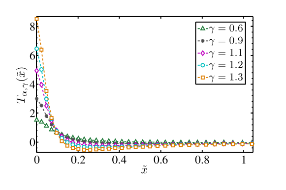
Figure 1: $T_{\alpha,\gamma}(\tilde{x})$ for $\alpha=0.5$, and for various $\gamma$ values. The $T_{\alpha,\gamma}(\tilde{x})$ values were calculated both by numerical inverse Fourier transform of the expression in Eq. (17) (markers) and by calculating the series expansion in Eq. (29) with $2\cdot 10^{5}$ terms (dashed lines). Note that we only illustrate the regime $\gamma>\alpha$, since these are the terms that appear in our series expansion.

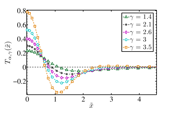
Figure 2: $T_{\alpha,\gamma}(\tilde{x})$ for $\alpha=1.3$, and for various $\gamma$ values. The $T_{\alpha,\gamma}(\tilde{x})$ values were calculated as in Fig. 1.

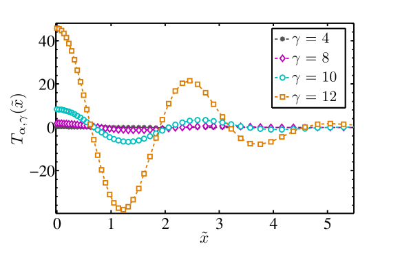
Figure 3: $T_{\alpha,\gamma}(\tilde{x})$ for $\alpha=2$ and even $\gamma$. These functions corresponds to the Gauss-Hermite functions. The $T_{\alpha,\gamma}(\tilde{x})$ values were calculated as in Fig. 1.

$\gamma$ affects the amplitude of $T_{\alpha,\gamma}(\tilde{x})$, i.e., the maximal (at $\tilde{x}=0$) and minimal (negative) values of $T_{\alpha,\gamma}(\tilde{x})$. One has to keep in mind that for $\gamma\rightarrow 0$ we get $T_{\alpha,\gamma}(\tilde{x})\rightarrow L_{\alpha}(\tilde{x})$, which is always positive. This implies that as $\gamma$ decreases the negative area also decreases, and since $\int_{0}^{\infty}T_{\alpha,\gamma}(\tilde{x})d\tilde{x}=0$ (for all $\gamma$ except for $\gamma=0$) since $\gamma=0$ yields a “pure” Lévy $\alpha$-stable density function which is normalized and the additional terms in the series must preserve the normalization, so that the integral over them must vanish. As can be seen in Fig. 1 and Fig. 2, when $\gamma$ decreases, both the positive and negative parts of $T_{\alpha,\gamma}(\tilde{x})$ decrease, and in addition the value of $\tilde{x}$ where $T_{\alpha,\gamma}(\tilde{x})$ crosses the $\tilde{x}$-axis increases (so that for $\gamma\rightarrow 0$ this value should go to infinity, to recover the positive definite $L_{\alpha}(\tilde{x})$ PDF).

When trying to characterize the effect of increasing $\alpha$ on $T_{\alpha,\gamma}$, we first refer to the well studied special case of $\gamma=0$. In this case, for $\alpha<2$ we get $T_{\alpha,\gamma}(\tilde{x})=L_{\alpha}(\tilde{x})$. Increasing $\alpha$ lowers the central peak and widens the central region of the density function until for $\alpha=2$ this term becomes a Gaussian. The same behavior also holds for $\gamma>0$ where increasing $\alpha$ makes the central peak lower, but the central region becomes wider. The value of $\tilde{x}$ where $T_{\alpha,\gamma}(\tilde{x})$ crosses the $\tilde{x}$-axis (which for the positive definite Lévy and Gaussian is going to infinity) increases as can be seen in Fig. 4.

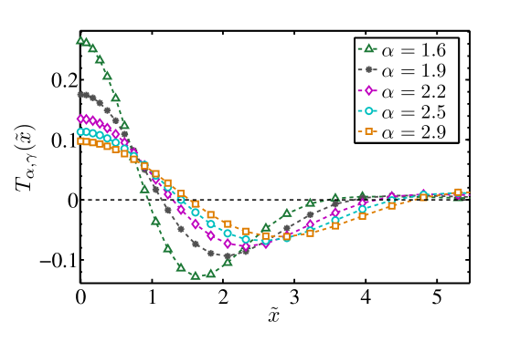
Figure 4: $T_{\alpha,\gamma}(\tilde{x})$ for $\gamma=3$ and various $\alpha$ values. The $T_{\alpha,\gamma}(\tilde{x})$ values were calculated as in Fig. 1.

III.3 Leading Order Fractional Edgeworth Expansion

Our approach for analyzing $w_{S}(x)$ both in the Gaussian and Lévy regimes is based on the fact that higher terms in the series expansion in Eq. (20) decrease more rapidly with $n$. We first consider a case where the Gaussian CLT applies, however, ${w}(x)\sim x^{-(\alpha+1)}$, where $\alpha>2$, so that sufficiently high order moments diverge. The truncated Edgeworth expansion will not give a good estimate of the tail of the PDF. The tail is described by non-analytical terms in the $k$ expansion, while the Gaussian CLT and the truncated Edgeworth expansion rely on analytical terms of the type $k^{2n}\exp(-k^{2})$ when $n$ is an integer. For example, the function $w(x)=3/2{\pi}(1+x^{6})$ is expanded in the Fourier space to:

$$\tilde{w}(k)=1-\frac{k^{2}}{4}+\frac{k^{4}}{24}-\frac{|k|^{5}}{80}+...$$ (30)

where the three terms (up to the $k^{4}$ term) are analytic, and the terms from the $|k|^{5}$ belong to the non-analytical part.

In the leading order fractional Edgeworth expansion we neglect all terms in the series that are higher than the first non-analytic term. In the Lévy regime, all the terms are non-analytic ($\alpha<2$), since even the second moment diverges and in this regime we take only the first term of the series. In the Gaussian regime (finite variance, $\alpha=2$), however, we need to take all the analytic terms first (the truncated Edgeworth series), but since these terms do not capture the behavior of the (heavy-) tailed nature of the $w(x)$ (its diverging moments) we still need to add the first non-analytic term in order to capture the power-law decay of the tails.

In the latter case (Gaussian regime), for PDFs that decay as $Ax^{-(1+\alpha)}$ ($\alpha>2$) for large $x$, this approach yields:

$${\tilde{w}_{S}}(k)=e^{-\sigma^{2}k^{2}/{2}}\left[1+\sum_{\nu=1}^{\nu<\alpha}P_{2\nu}(ik)n^{-\nu}+\frac{1}{n^{\alpha/2-1}}\xi(k)\right],$$ (31)

where $P_{\nu}$ is defined in Eq. (8) and the summation of the Edgeworth part (second term in the brackets) is only over even values of $\nu$ (because of the symmetric nature of $w(x)$) and is over values of $\nu$ up to but not including $\alpha$. The last term is given by:

$$\xi(k)=\left\{\begin{array}[]{ll}\rule[5.0pt]{0.0pt}{10.0pt}-\frac{A\pi}{\Gamma(\alpha+1)\sin(\alpha\pi/2)}|k|^{\alpha},&\alpha\neq 2n\\ \rule[5.0pt]{0.0pt}{15.0pt}\frac{2A\pi(-1)^{\alpha/2}}{\Gamma(\alpha+1)}|k|^{\alpha}\log|k|,&\alpha=2n\end{array}\right.$$ (32)

The corresponding $w_{S}(x)$ is then:

$$w_{S}(x)=Z_{\sigma}(x)+\sum_{\nu=1}^{\nu<\alpha}\frac{\zeta_{2\nu}\left(\frac{\sqrt{2}x}{\sigma}\right)}{n^{\nu}}+\frac{2^{(1+\alpha)/2}b_{\alpha}}{n^{\alpha/2-1}\sigma^{1+\alpha}}T_{2,\alpha}\left(\frac{\sqrt{2}x}{\sigma}\right).$$ (33)

where $\zeta_{\nu}$ is defined using the $T_{\alpha,\gamma}$ terms:

$$\zeta_{\nu}\left(\frac{\sqrt{2}x}{\sigma}\right)=\left(\frac{\sqrt{2}}{\sigma}\right)^{\nu+2r+1}\sum_{\{k_{m}\}}T_{2,\nu+2r}\left(\frac{\sqrt{2}x}{\sigma}\right)\prod_{m=1}^{\nu}\frac{1}{k_{m}!}\left(\frac{\kappa_{m+2}}{(m+2)!}\right)^{k_{m}},$$ (34)

where $r$ and the sets $\{k_{m}\}$ are the same as in Eq. (4), from Eq. (32):

$$b_{\alpha}=\left\{\begin{array}[]{ll}\rule[5.0pt]{0.0pt}{10.0pt}-\frac{A\pi}{\Gamma(\alpha+1)\sin(\alpha\pi/2)},&\alpha\neq 2n\\ \rule[5.0pt]{0.0pt}{15.0pt}\frac{2A\pi(-1)^{\alpha/2}}{\Gamma(\alpha+1)},&\alpha=2n\end{array}\right.$$ (35)

where for the case of even $\alpha$, the $T_{2,\alpha}$ is defined as in Eq. (27).

In the Lévy regime ($0<\alpha<2$), as mentioned, all the cumulants diverge. As a consequence there are no terms in the Edgeworth expansion, and only the non-analytic terms exists. We used the same scheme as in Eq. (14) to Eq. (20). In Eq. (15) we expand $\tilde{w}_{S}(k)$ in a power series in two stages: first, we use the expansion $\tilde{w}(k)=1+a_{1}|k|^{\alpha_{1}}+a_{2}|k|^{\alpha_{2}}+O(|k|^{\alpha_{2}})$, where $\alpha\equiv\alpha_{1}$, $a\equiv-a_{1}$ is a positive constant depending only on $\alpha$, $a=\pi/[\Gamma(\alpha+1)\sin(\alpha\pi/2)]$ Klafter and Sokolov [2011], $\alpha_{2}>\alpha$, and $a_{2}$ is a constant depending on the explicit form of $w(x)$. Then we expand the $\ln(1+x)\simeq x-x^{2}/2$ and truncate the series after its second term:

$$\tilde{w}_{S}(k)\simeq e^{-a|k|^{\alpha}}\left[1+C_{n}|k|^{\gamma}\right]$$ (36)

where:

$$\gamma=\begin{cases}\alpha_{2},&\alpha_{2}<2\alpha\\ 2\alpha,&\alpha_{2}\geq 2\alpha\\ \end{cases},$$ (37)

and:

$$C_{n}=\frac{1}{n^{\gamma/\alpha-1}}\begin{cases}a_{2},&\alpha_{2}<2\alpha\\ -{a^{2}}/{2},&\alpha_{2}>2\alpha\\ a_{2}-{a^{2}}/{2},&\alpha_{2}=2\alpha\end{cases},$$ (38)

and the leading order fractional Lévy Edgeworth takes the form:

$$w_{S}(x)\simeq\frac{1}{a^{1/\alpha}}\left[L_{\alpha}(a^{-1/\alpha}x)+\frac{C_{n}}{a^{\gamma/\alpha}}T_{\alpha,\gamma}(a^{-1/\alpha}x)\right],$$ (39)

where $\gamma$ and $C_{n}$ depend on the explicit form of $w(x)$ as in Eq. (37) and Eq. (38). The possible values of $\gamma$ for a given $\alpha$ value taken from Eq. (37) are shown in Fig. 5. As discussed in the previous section, $T_{\alpha,\gamma}(x)$ is positive in its central part, and negative in the edges. The effect of the leading order fractional Lévy Edgeworth term on the PDF depends on the coefficient $C_{n}$ in Eq. (39). If $C_{n}$ is positive, this correction will increase the probability for the small $x$ values, and decrease the probability of large values. If $C_{n}$ is negative, the effect will be opposite.

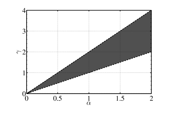
Figure 5: The strip of possible $\gamma$ values for the first correction term, $T_{\alpha,\gamma}(\tilde{x})$ as a function of $\alpha$ shown as the shaded area in the figure.

IV Example: Cold Atoms in Optical Lattice

An important physical application of the above methods is in the field of atoms in an optical lattice undergoing diffusion in momentum space. Castin et al. [1991]; Marksteiner et al. [1996]. It has been shown that the atoms are subjected to a cooling force (in dimensionless units Kessler and Barkai [2010]) of the form:

$$F(p)=-\frac{p}{1+p^{2}},$$ (40)

where $p$ is the dimensionless momentum of the atom. This cooling force acts to decrease the momentum of the atom to zero while the fluctuations in momentum can be treated as a diffusive process (in momentum space) causing heating. In the semi-classical picture, one may describe the PDF of the momentum of an atom as the solution of a Fokker-Planck equation (given, e.g., in Kessler and Barkai [2010]). The equilibrium solution of this equation, $W_{eq}(p)$, is given by:

$$W_{eq}(p)=\mathcal{N}(1+p^{2})^{-1/(2D)}.$$ (41)

Here, $\mathcal{N}=\Gamma(\frac{1}{2D})/[\sqrt{\pi}\Gamma(\frac{1-D}{2D})]$ is a normalization constant, and $D$, the dimensionless diffusion constant, is defined by $D=cE_{R}/U_{0}$, where $U_{0}$ is the depth of the optical potential, $E_{R}$ the recoil energy depends on the atomic transition involved Cohen-Tannoudji and Phillips [1990]; Castin et al. [1991]. Laser cooling experiments indeed show this kind of steady state solution, where $D$ can be tuned during the experiment to achieve different steady state behavior Douglas et al. [2006]. The transition between normal (Gaussian) and anomalous (Lévy) diffusion in space is also observed Katori et al. [1997].

In what follows, we derive the approximate density function for the sum of the momenta of $n$ such atoms scaled by the appropriate $n^{1/\alpha}$ where $\alpha$ depends on the value of $D$, as will be explained later. For different values of $D$ there are three different types of $W_{eq}(p)$. For $D>1$ this function is not normalizable, and we will not analyze this case further. For $D<1$, however, there are still two possibilities, the Gaussian regime $0<D<1/3$ where the variance is finite, $\sigma^{2}=D/(1-3D)$, and the Lévy regime $1/3<D<1$, where the variance diverges. The characteristic function of $W_{eq}(p)$ is:

$$\tilde{w}(k)=\frac{2^{3/2-1/2D}}{\Gamma(1/2D-1/2)}|k|^{\frac{1}{2D}-\frac{1}{2}}K_{\frac{1}{2D}-\frac{1}{2}}(|k|),$$ (42)

where $K$ is the modified Bessel function of the second kind, defined as:

$$K_{\nu}(k)=\frac{\pi}{2}\frac{I_{-\nu}(k)-I_{\nu}(k)}{\sin(\nu\pi)},$$ (43)

and $I_{\nu}(k)$ is the modified Bessel function of the first kind. with the Froebenius expansion:

$$I_{\nu}(k)=\sum_{m=0}^{\infty}\frac{1}{m!\Gamma(m+\nu+1)}\left(\frac{k}{2}\right)^{2m+\nu}.$$ (44)

This series expansion is valid only for non-integer values of $\nu$. The integral $\nu$ case can be treated as the limit of the non-integral one using the methods in Abramowitz and Stegun [1972]. Integer values of $\nu$ appear when $D=1/(2n+1)$ ($n$ is a positive integer) i.e, in the Gaussian regime. For these specific $D$ values the series expansion of the modified Bessel $K$ contains logarithmic terms. For example, for $D=1/5$ we get:

$$\tilde{w}(k)=\frac{1}{4}k^{2}K_{2}(|k|)=1-\frac{k^{2}}{4}+\frac{1}{64}\bigg{(}3-4\gamma_{E}+4\log(2)-4\log(|k|)\bigg{)}k^{4}+...,$$ (45)

where $\gamma_{E}\simeq 0.5772$ is the Euler–Mascheroni constant. As mentioned above, these cases will not be treated here.

For this kind of power-law decaying PDF, even in the Gaussian regime that will be presented below, the Edgeworth series does not converge, since higher moments do not exist. Using Eq. (44) and defining $\nu=1/2D-1/2$ we get:

$$\tilde{w}(k) =\sum_{m=0}^{\infty}\bigg{[}\frac{\Gamma(1-\nu)}{m!\Gamma(m-\nu+1)}\left(\frac{|k|}{2}\right)^{2m}-\frac{\Gamma(1-\nu)}{m!\Gamma(m+\nu+1)}\left(\frac{|k|}{2}\right)^{2(m+\nu)}\bigg{]}$$

$$=1-\frac{\Gamma(1-\nu)}{\Gamma(1+\nu)2^{2\nu}}|k|^{2\nu}+\frac{\Gamma(1-\nu)}{\Gamma(2-\nu)2^{2}}|k|^{2}+\ldots.$$ (46)

To analyze this further, we need to break it down to two cases. When $2\nu>2$ (which occurs when $0<D<1/3$) we are in the Gaussian regime, with the leading order term $\exp(-\sigma^{2}k^{2}/2)$ where $\sigma^{2}=D/(1-3D)$.

$${\tilde{w}_{S}}(k)\simeq e^{-\sigma^{2}k^{2}/2}\bigg{[}1+\sum_{n=1}^{n<2\nu}P_{2n}(ik)-\frac{\Gamma(1-\nu)}{\Gamma(1+\nu)2^{2\nu}n^{\nu-1}}|k|^{2\nu}\bigg{]},$$ (47)

where $P_{2n}(ik)$ is defined by Eq. (8) and the sum runs over all the even powers of $k$ from $4$ to the maximal even integer smaller than $2\nu$. This truncated Edgeworth correction will vanish (so that there are no analytic terms) at the point where the $4$th moment of $w(x)$ diverges, (i.e., for $D>1/5$). It is easy to show that the last term in this equation (the correction term) is a special case of Eq. (32).

When $2\nu<2$ (when $1/3<D<1$) we are in the Lévy regime, and $\alpha=2\nu=1/D-1$, so that the leading order fractional Lévy Edgeworth expansion of $\tilde{w}_{S}(k)$ takes the form:

$${\tilde{w}_{S}}(k)\simeq e^{-a_{\alpha}|k|^{\alpha}}\left\{\begin{array}[]{ll}\rule[5.0pt]{0.0pt}{10.0pt}\mbox{ }\left[1+\frac{\Gamma(1-\alpha/2)}{\Gamma(2-\alpha/2)2^{2}n^{2/\alpha-1}}|k|^{2}\right],&\alpha>1\\ \rule[5.0pt]{0.0pt}{15.0pt}\left[1-\frac{\Gamma^{2}(1-\alpha/2)}{\Gamma^{2}(1+\alpha/2)2^{2\alpha+1}n}|k|^{2\alpha}\right],&\alpha<1\\ \rule[5.0pt]{0.0pt}{15.0pt}1\mbox{ },&\alpha=1\end{array}\right.$$ (48)

where $a_{\alpha}\equiv{\Gamma(1-\alpha/2)}/{\Gamma(1+\alpha/2)2^{\alpha}}$ and the leading term here agrees with Eqs. (36)-(38). In the last case, corresponding to $D=1/2$, there is no correction term, since in this case the single atom momentum distribution (in Eq.(41)) already gives the Cauchy distribution, i.e., the $L_{1}(x)$ which is stable.

IV.1 Gaussian Regime

In order to find $W_{eq}(\mathcal{P})$, the PDF of the random variable $\mathcal{P}\equiv\sum_{j=1}^{n}p_{j}/n^{1/2}$, we calculate numerically the inverse Fourier transform of $\tilde{w}(k/n^{1/2})^{n}$ using Eq. (42). In what follows we refer to this result as the exact solution, $W_{eq}(\mathcal{P})$.

In the Gaussian regime, (even) moments exist only up to the highest integer that is smaller than $\frac{1}{D}-1$. For example, for $1/5<D<1/3$ where even the $4$th moment doesn’t exist, the truncated Edgeworth reduces to the CLT. In Fig. 6 and Fig. 7 we compare the CLT $Z_{\sigma}(\mathcal{P})=\frac{1}{\sqrt{2\pi\sigma^{2}}}\exp(-\sigma^{2}\mathcal{P}^{2}/2)$, the exact solution $W_{eq}(\mathcal{P})$, the truncated Edgeworth series $W^{(te)}(\mathcal{P})$, and the fractional Gauss Edgeworth expansion, $W^{(fge)}(\mathcal{P})$, for $D=1/6$ (corresponding to $\sigma^{2}=1/3$) and $D=0.3$ (corresponding to $\sigma^{2}=3$). Using Eq. (47) without the non-analytic term (and transforming back to $P$ space), the truncated Edgeworth expansion in this case takes the form:

$$W^{(te)}(\mathcal{P}) =Z_{1/\sqrt{3}}(\mathcal{P})+\frac{2(\sqrt{6})^{5}}{3\cdot 4!n}T_{2,4}(\sqrt{6}\mathcal{P})$$

$$=\sqrt{\frac{3}{2\pi}}e^{-3\mathcal{P}^{2}/2}\bigg{[}1+\frac{3}{4n}\Big{(}1-6\mathcal{P}^{2}+3\mathcal{P}^{4}\Big{)}\bigg{]}.$$ (49)

Adding the first non-analytic term in Eq. (47) (and transforming back to $\mathcal{P}$ space) gives:

$$W^{(fge)}(\mathcal{P}) =W^{(te)}(\mathcal{P})-\frac{2^{3}3^{3}}{45n^{3/2}}T_{2,5}(\sqrt{6}\mathcal{P})$$

$$=W^{(te)}(\mathcal{P})-\frac{3}{5\pi n^{3/2}}\bigg{[}8+9\mathcal{P}^{2}(-3+\mathcal{P}^{2})-3\sqrt{6}\mathcal{P}\bigg{(}5-10\mathcal{P}^{2}+3\mathcal{P}^{4}\bigg{)}\textrm{Daw}\bigg{(}\sqrt{\frac{3}{2}}\mathcal{P}\bigg{)}\bigg{]}.$$ (50)

By asymptotic expansion of the Dawson function for large $\mathcal{P}$ values, we find that $W^{(fge)}(\mathcal{P})$ decays as $\sim 1/\mathcal{P}^{6}$ as expected for $D=1/6$, since $W_{eq}(p)\sim p^{-1/D}$ in Eq. (41). As can be seen in Fig. 6, the truncated Edgeworth expansion fits the exact solution better than the CLT, but for the tails of the density function this approximation breaks down. Adding the non-analytic term to the Edgeworth series corrects this and the two curves coincide even for the moderate $n=20$. As $D$ approaches $1/3$, the fractional Gauss Edgeworth approximation converges to the exact solution for higher $n$ values, while the truncated Edgeworth correction cannot recover the exact solution behavior even for much higher $n$ values, and even the central part of the truncated Edgeworth density function is significantly different from the exact solution as can be seen, for example, in Fig. 7 for $n=200$.

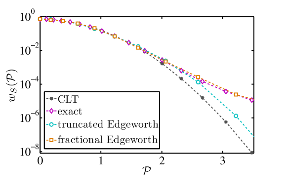
Figure 6: $w_{S}(\mathcal{P})$ for $D=1/6$ and $n=20$ drawn in a semi-log scale. A comparison between the CLT, the exact solution, the truncated Edgeworth expansion and the (leading order) fractional Gauss Edgeworth expansion.

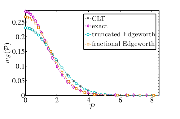
Figure 7: $w_{S}(\mathcal{P})$ for $D=0.3$ and $n=200$. A comparison between the CLT, the exact solution, the truncated Edgeworth expansion (coincides with the CLT for $D=0.3$) and the (leading order) fractional Gauss Edgeworth expansion.

Since for $n\rightarrow\infty$ all the above PDFs coincide, and the higher $n$ is, the closer the PDFs will be to each other, a good measure for evaluating the quality of these approximations is to calculate $n^{*}$ for which the approximated PDF is close enough to the exact solution. We calculate $n^{*}$ as the $n$ for which:

$$\int_{-\infty}^{\infty}\big{(}W_{ap}(\mathcal{P})-W_{eq}(\mathcal{P}\big{)}^{2}d\mathcal{P}\leq\varepsilon_{cut},$$ (51)

where $W_{ap}(\mathcal{P})$ corresponds to $W^{(te)}(\mathcal{P})$ or $W^{(fge)}(\mathcal{P})$, and $\varepsilon_{cut}$ is a tunable threshold.

In Fig. 8 we examine the convergence of the approximate PDFs to the exact solution for different $D$ values. As can be seen, whereas the convergence of the truncated Edgeworth expansion becomes very slow as $D\rightarrow 1/3$ (high values of $n^{*}$), the (first-term) fractional Gauss Edgeworth approximation yields much faster convergence (smaller values of $n^{*}$). The reason for this slow convergence of the truncated Edgeworth series is that the Edgeworth series is an expansion around a Gaussian. The inverse Fourier transform of the Edgeworth terms has the form of $H_{n}(\mathcal{P}/\sigma)Z_{\sigma}(\mathcal{P})$ where $H_{n}$ is the Hermite polynomial, and for large values of $\mathcal{P}$ the tails behavior is controlled by the exponential decay which does not mimic the power-law decay of the exact solution. The non-analytic expansion indeed decays according to the exact solution’s power law, as we will now show. The inverse Fourier transform of the non-analytic term is given by the integral:

$$\int_{0}^{\infty}dk\,k^{\gamma}e^{-\sigma^{2}k^{2}/(2)}\cos(k\mathcal{P})=\frac{1}{2\sigma^{(\gamma+1)/2}}\Gamma(\gamma+1)e^{-\mathcal{P}^{2}/4\sigma^{2}}\bigg{[}D_{-(\gamma+1)}(-i\mathcal{P}/\sigma)+D_{-(\gamma+1)}(i\mathcal{P}/\sigma)\bigg{]}$$ (52)

where $\gamma=1/D-1$, $D_{a}(z)$ is the parabolic-cylindric function Abramowitz and Stegun [1972], which for large $z$ goes to $\exp(-z^{2}/4)z^{a}$. Substituting in this large $\mathcal{P}$ asymptotic behavior, the Gaussian term cancels and we are left with a power-law decay where $T_{2,\gamma}(\mathcal{P})\sim 1/\sigma^{\gamma+1}\Gamma(\gamma+1)\mathcal{P}^{-(\gamma+1)}$. As can be seen in Fig. 7 this addition of the non-analytic term gives a pretty good approximation to the exact solution suggesting that the power-law decay of the exact solution decays as the expected $\mathcal{P}^{-(\gamma+1)}$.

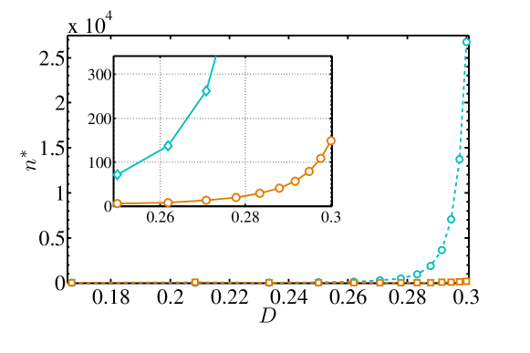
Figure 8: $n^{*}$ for different $D$ values in the Gaussian regime, where $n^{*}$ measures the convergence of the truncated Edgeworth expansion (blue) and the (leading order) fractional Gauss Edgeworth expansion (orange) to the exact solution. $\varepsilon_{cut}=3\cdot 10^{-4}$. The figure illustrates that the truncated Edgeworth does not work so well compared to the fractional Gauss Edgeworth expansion. In the inset we show that the leading order fractional Gauss Edgeworth indeed has a slight increment in $n^{*}$ when $D$ approaches $1/3$.

The Edgeworth and the non-analytic corrections are still expansions around the Gaussian, but as $D$ approaches $1/3$ we move from the Gaussian regime towards the Lévy regime. As $D\rightarrow 1/3$ the convergence to the exact solution becomes very slow, and only for extremely high $n$ do the PDFs approach the exact solution. For all values of $D$, the (first-term) non-analytic approximation yields faster convergence (smaller value of $n^{*}$) than the truncated Edgeworth one due to the transition from exponential to power-law decay.

For $D\rightarrow 1/3$ from below, even though the variance of $W_{eq}(p)$ is finite, the convergence of the exact solution to a Gaussian is seen only for extremely high $n$ values (see Fig. 8), because the variance grows as $\sigma^{2}=D/(1-3D)$ which diverges at $D=1/3$.

IV.2 Lévy Regime

For $1/3<D<1$, where the variance diverges, the basin of attraction of the PDF is the Lévy $\alpha$-stable density function, where for cold atoms, $\alpha=\frac{1}{D}-1$. We will derive, therefore, the PDF of the random variable $\mathcal{P}\equiv\sum_{j=1}^{n}p_{j}/n^{1/\alpha}$. As we have discussed, unlike the expansion in the Gaussian regime, the series in this regime is entirely non-analytic in nature. Although for large $n$ the exact solution tends to the Lévy density function, when $D$ approaches $1/3$ (from above in the Lévy regime), the $n$ needed for this convergence grows asymptotically. This is clearly shown in Fig. 9 where we’ve plotted $n^{*}$ (defined as above), comparing the leading order fractional Lévy Edgeworth and the exact solution. Even though for large $n$ the PDF goes to the pure Lévy $\alpha$-stable density function, when $D\rightarrow 1/3$ this convergence becomes very slow.

We will now show this slow convergence effect through the following example cases. When $D=3/7$, corresponding to $\alpha=4/3$, $\gamma=2$, $a\simeq 1.178$ and $C_{n}=3/(4n^{1/2})$ and using Eqs. (36)-(39):

$$w_{S}(\mathcal{P})\simeq\frac{1}{a^{3/4}}\left[L_{\frac{4}{3}}(a^{-3/4}\mathcal{P})+\frac{C_{n}}{a^{3/2}}T_{\frac{4}{3},2}(a^{-3/4}\mathcal{P})\right].$$ (53)

For $D=11/30$ which is much closer to $1/3$, we get the corresponding $\alpha=19/11$, $\gamma=2$, $a\simeq 2.186$ and $C_{n}=11/(6n^{3/19})$ yielding:

$$w_{S}(\mathcal{P})\simeq\frac{1}{a^{11/19}}\left[L_{\frac{19}{11}}(a^{-11/19}\mathcal{P})+\frac{C_{n}}{a^{22/19}}T_{\frac{19}{11},2}(a^{-11/19}\mathcal{P})\right].$$ (54)

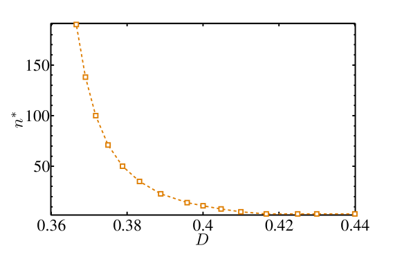
Figure 9: $n^{*}$ values for different $D$ values in the Lévy regime, where $n^{*}$ measures the convergence of the leading order fractional Edgeworth expansion to the exact solution. $\varepsilon_{cut}=3\cdot 10^{-4}$.

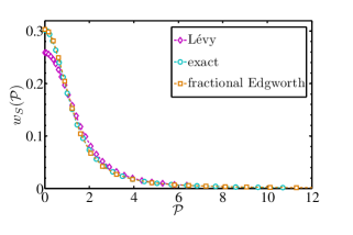
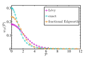
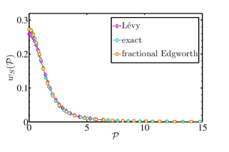
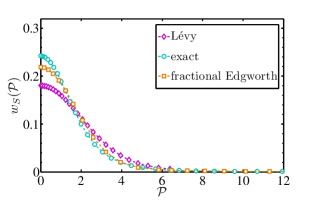
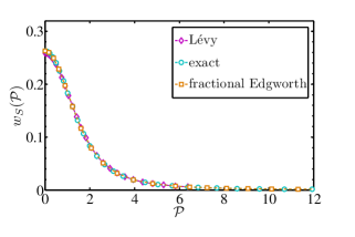
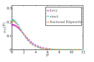
Figure 10: $w_{S}(\mathcal{P})$ for $D=3/7$, corresponding to $\alpha=4/3$ (left hand side) and $D=11/30$, corresponding to $\alpha=19/11$ (right hand side) for $n=10$ (first row), $n=100$ (second row) and $n=1000$ (third row). A comparison between $L_{\alpha}(x)$, the exact solution and the leading order fractional Lévy Edgeworth expansion.

In Fig. 10 we plot $w_{S}(\mathcal{P})$ for the above examples for different $n$ values ($n=10,100,1000$) in order to compare the convergence to the exact solution as $D$ approaches $1/3$. It can be observed that for $D=3/7$, even for the moderate $n=10$ the correction gives much better convergence to the exact solution, compared to the $\alpha$-Lévy stable PDF. Increasing $n$, both the exact solution and the leading term fractional Edgeworth approximation converge to the $\alpha$-Lévy stable PDF. Nevertheless, the fractional Lévy Edgeworth approximation still approximates the exact solution better than the $\alpha$-Lévy stable PDF. For $D=11/30$, however, the convergence is much slower. In the range of $n$ presented here, both the Lévy density function and the corrected solution do not coincide with the exact solution, even though the fractional Edgeworth expansion gives a better approximation to the exact solution than the Lévy density function. For much higher $n$ values, however, the approximation Eq.(54) indeed coincides (up to our numeric accuracy) with the exact solution, as shown in Fig. 9.

In contrast to the Gaussian regime where the non-analytic term corrects the tail’s behavior from exponential decay to a power-law one, in the Lévy regime, for high $\mathcal{P}$ values the density function already decays with the same power-law as the Lévy, and the leading order fractional Lévy Edgeworth correction term takes care mostly of the center of the density function. This behavior of the tails is clearly shown in Fig. 11, where we plotted $w_{S}(\mathcal{P})$ for $D=11/30$ and $n=100$ in a semi-log plot,

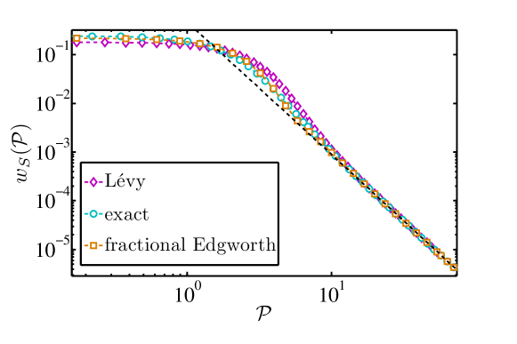
Figure 11: $w_{S}(\mathcal{P})$ for $D=11/30$ and $n=100$. A comparison between $L_{\alpha}(x)$, the exact solution and the leading order fractional Lévy Edgeworth expansion in a log-log plot, in order to highlight the power-low decaying behavior of the tails. The black dashed line has the expected slope of $\alpha+1\simeq 3$ for $D=11/30$, and all of these curves converge to this slope for large $\mathcal{P}$.

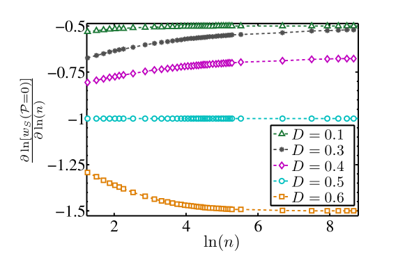
Figure 12: $\frac{\partial\log\left[w_{S}(\mathcal{P}=0)\right]}{\partial\log\left(n\right)}$ as a function of $\log\left(n\right)$ for different $D$ values. each curve converges asymptotically to its suitable $\alpha$. The curves corresponding to $D=0.1$ and $D=0.3$ tend asymptotically to $-0.5$ as expected in the Gaussian regime, while the curve corresponding to $D=0.3$ converges for much higher $n$ values. For $D$ equals $0.4$ ,$0.5$ and $0.6$ the curves tend asymptotically to $-1/\alpha$, i.e., to $-2/3$, $-1$ and $-3/2$ respectively. In the Lévy regime, $D=0.5$ gives a pure Lévy density function already for $n=1$. For higher and lower $D$ values in this regime the convergence becomes slower, and higher values of $n$ are needed for the asymptotic convergence.

A way to show the convergence of the central part of these PDFs to their basin of attraction is to calculate the dependence of $w_{S}(\mathcal{P})$ on $n$ at $\mathcal{P}=0$ Mantegna and Stanley [1994]. It will be more instructive for this purpose (in order to show the different attractors of the Gaussian and Lévy regimes) to use the PDF of the sum $\mathcal{P}=\sum_{i=1}^{n}p_{i}$ instead of normalizing it by $n$ to the appropriate power. For pure $Z_{\sigma}(\mathcal{P})$ and $L_{\alpha}(\mathcal{P})$ functions, $w_{S}(\mathcal{P}=0)\propto n^{-1/\alpha}$ (where for $Z_{\sigma}(\mathcal{P})$ we use $\alpha=2$). By plotting the dependence of $w_{S}(\mathcal{P}=0)$ on $n$ one can see how fast the density function converges to the stable density function. In Fig. 12 we plot $\partial\log\left(w_{S}(\mathcal{P}=0)\right)/\partial\log\left(n\right)$ as a function of $\log\left(n\right)$ which for large $n$ goes to $-1/\alpha$. As can be seen, for $0<D<1/3$ the curves converge asymptotically to $-1/2$ while for $1/3<D<1$ each curve converges to its appropriate $-1/\alpha=D/(D-1)$. Also, one may observe that as $D$ approaches $1/3$ from both sides, the convergence of the curves become much slower.

V Summary

In this article we have generalized the classical Edgeworth expansion for finite $n$ to PDFs which converge to the $\alpha$-stable Lévy density functions. In order to do this we used a generalized Fourier series including fractional powers of $k$ and showed that the inverse Fourier transform of this series may be written by means of a series of fractional derivatives of the Lévy PDF and its conjugate, $R_{\alpha}(x)$ (Eq. (18)). This generalization is shown to be universal since it also gives the classical Edgeworth series for PDFs in the Gaussian regime when all the moments exist, and the fractional Gauss Edgeworth expansion developed by Lam, et al Lam et al. [2011]. for PDFs with finite variance but diverging moments.

For the correction terms we introduced a new family of special functions, $T_{\alpha,\gamma}(x)$ Eq. (17), for which the Gaussian, the Lévy and the Hermite-Gauss functions are special cases. We also represented these functions as $H$-Fox functions via the Mellin-Barnes integral. We investigated the behavior of these functions in the context of our correction terms (for specific values of $\alpha$ and $\gamma$).

We have applied our results to the sum of momenta of cold atoms, and showed that taking even only the first correction term of our fractional series (leading term approximation) already gives much better matching to the exact solution for small values of $n$. At the transition between Gauss to Lévy behaviors, we have found very slow convergence to the asymptotic result.

VI Acknowledgments

This work is supported by the Israel Science Foundation (ISF).

Appendix A $T_{\alpha,\gamma}(x)$ as the $H$-Fox Function

A.1 The $H$-Fox function

Fox Fox [1961]; Braaksma [1936] defined the $H$-function by

$$H^{m,n}_{p,q}(z)=\frac{1}{2\pi i}\int_{L}\chi(s)z^{s}ds,$$ (55)

where $L$ is a path in the complex plane $\mathbb{C}$ to be described later, $z=\exp(\log|z|+i\;\arg z)$ and the integral density $\chi(s)$ is given by

$$\chi(s)=\frac{A(s)B(s)}{C(s)D(s)}=\frac{\prod_{j=1}^{m}\Gamma(b_{j}-B_{j}s)\prod_{j=1}^{n}\Gamma(1-a_{j}+A_{j}s)}{\prod_{j=m+1}^{q}\Gamma(1-b_{j}+B_{j}s)\prod_{j=n+1}^{p}\Gamma(a_{j}-A_{j}s)},$$ (56)

$n$,$m$,$p$,$q$ are integers satisfying

$$0\leq n\leq p,\quad 1\leq m\leq q,$$

$A_{j},B_{j}$ are positive numbers and $a_{j},b_{j}$ are in general complex numbers. When no elements appear in one of the multiplications in Eq. 56 one gets an empty product which is taken to equal unity:

$$m=0\rightarrow A(s)=1,\quad n=0\rightarrow B(s)=1,\quad m=q\rightarrow C(s)=1,\quad n=p\rightarrow D(s)=1.$$

Since $H^{m,n}_{p,q}(z)$ depends on the sets $\{a_{i},A_{i}\}$ and $\{b_{i},B_{i}\}$, a common notation for $H^{m,n}_{p,q}(z)$ is:

$$H^{m,n}_{p,q}(z)\equiv H^{m,n}_{p,q}\left[{z}\bigg{|}\begin{array}[]{cc}{(a_{j},A_{j})_{j=1,\ldots,p}}\\ {(b_{j},B_{j})_{j=1,\ldots,q}}\end{array}\right]\\$$ (57)

This representation of the $H$-Fox function via an integral involving products and ratios of Gamma functions is known as the Mellin-Barnes integral Marichev [1983]; Paris and Kaminski [2001]. The singular points of the kernel $\chi(s)$ are the poles of the Gamma functions in $A(s)$ and $B(s)$, which are assumed to not coincide. Denoting the sets of poles by $P(A)$ and $Q(B)$ respectively, $P(A)\cap Q(B)=\emptyset$. The conditions for the existence of the $H$-Fox function can be determined by examination of the convergence of the integral in Eq. (55), which depends on the selection of the contour $L$ and on certain relations between the parameters $\{a_{i},A_{i}\}$ where $i=1,\ldots,p$ and $\{b_{j},B_{j}\}$ where $j=1,\ldots,q$. The contour $L$ in Eq.(55) can be chosen as the contour in which all poles of $P(A)$ lie to its right and all poles of $Q(B)$ to lie its left while further $L$ runs from $c-i\infty$ to $c+i\infty$. Other kinds of Barnes-contours are also possible (see e.g., Braaksma [1936]; Mathai et al. [2009]).

It was shown by Braaksma Braaksma [1936] that the Mellin-Barnes integral in Eq. 55 makes sense and defines an analytic function of $z$ in the following two cases:

1. $$\mu=\sum_{i=1}^{q}B_{i}-\sum_{j=1}^{p}A_{j}>0,\quad\forall z\not=0$$ (58)

   .

2. $$\mu=0\quad and\quad 0\leq|z|\leq\delta\quad where\quad\delta=\prod_{i=1}^{q}(B_{i})^{B_{i}}\prod_{j=1}^{p}(A_{j})^{-A_{j}}.$$ (59)

The convergence and asymptotic expansions (for $z\rightarrow 0$ and $z\rightarrow\infty$) are determined by applying the residue theorem at the poles (which are by assumption simple poles) of the Gamma functions in $A(s)$ and $B(s)$.

The $H$-Fox function has a few properties which are important to our purposes:

1. The $H$-Fox function is symmetric in the pairs $(a_{1},A_{1}),\ldots,(a_{n},A_{n})$, likewise $(a_{n+1},A_{n+1}),\ldots,(a_{p},A_{p})$; in $(b_{1},B_{1}),\ldots,(b_{m},B_{m})$ and in $(b_{m+1},B_{m+1}),\ldots,(b_{q},B_{q})$.

2. If one of the $(a_{j},A_{j})$ $j=1,\ldots,n$, is equal to one of the $(b_{j},B_{j})$, $j=m+1,\ldots,q$ or one of the pairs $(a_{j},A_{j})$, $j=n+1,\ldots,p$ is equal to one of the $(b_{j},B_{j})$, $j=1,\ldots,m$ then the $H$-Fox function reduces to a lower order $H$-function, namely, $p$ and $q$, and $n$ (or $m$) decrease by unity. Provided that $n\geq 1$ and $q>m$ we have:

   $$H^{m,n}_{p,q}\left[z\bigg{|}\begin{array}[]{cc}{(a_{j},A_{j})_{1,p}}\\ {(b_{j},B_{j})_{1,q-1}(a_{1},A_{1})}\end{array}\right]=H^{m,n-1}_{p-1,q-1}\left[z\bigg{|}\begin{array}[]{cc}{(a_{j},A_{j})_{2,p}}\\ {(b_{j},B_{j})_{1,q-1}}\end{array}\right],$$ (60)

   $$H^{m,n}_{p,q}\left[z\bigg{|}\begin{array}[]{cc}{(a_{j},A_{j})_{1,p-1}(b_{1},B_{1})}\\ {(b_{1},B_{1})(b_{j},B_{j})_{2,q}}\end{array}\right]=H^{m-1,n}_{p-1,q-1}\left[z\bigg{|}\begin{array}[]{cc}{(a_{j},A_{j})_{1,p-1}}\\ {(b_{j},B_{j})_{2,q}}\end{array}\right]$$ (61)

3. $$z^{\sigma}H^{m,n}_{p,q}\left[{z}\bigg{|}\begin{array}[]{cc}{(a_{j},A_{j})_{1,p}}\\ {(b_{j},B_{j})_{1,q}}\end{array}\right]=H^{m,n}_{p,q}(z)=H^{m,n}_{p,q}\left[{z}\bigg{|}\begin{array}[]{cc}{(a_{j}+\sigma A_{j},A_{j})_{1,p}}\\ {(b_{j}+\sigma B_{j},B_{j})_{1,q}}\end{array}\right]$$ (62)

4. $$\frac{1}{c}H^{m,n}_{p,q}\left[{z}\bigg{|}\begin{array}[]{cc}{(a_{j},A_{j})_{1,p}}\\ {(b_{j},B_{j})_{1,q}}\end{array}\right]=H^{m,n}_{p,q}(z)=H^{m,n}_{p,q}\left[{z}\bigg{|}\begin{array}[]{cc}{(a_{j},cA_{j})_{1,p}}\\ {(b_{j},cB_{j})_{1,q}}\end{array}\right],\quad c>0$$ (63)

5. Another useful and important formula for the $H$-Fox function is

   $$H^{1,1}_{2,2}\left[z\bigg{|}\begin{array}[]{cc}{(a_{j},A_{j})_{1,p}}\\ {(b_{j},B_{j})_{1,q}}\end{array}\right]=H^{1,1}_{2,2}\left[\frac{1}{z}\bigg{|}\begin{array}[]{cc}{(1-b_{j},B_{j})_{1,q}}\\ {(1-a_{j},A_{j})_{1,p}}\end{array}\right],$$ (64)

This last relation enables us to transform an $H$-Fox function with $\mu<0$ and argument $z$ to one with $\mu>0$ and argument $1/z$.

A.2 Representation of $T_{\alpha,\gamma}(x)$

In order to represent $T_{\alpha,\gamma}(x)$ by the $H$-Fox function first we express $T_{\alpha,\gamma}(x)$ as a Mellin-Barnes integral. $T_{\alpha,\gamma}(x)$ is defined as the following inverse Fourier transform :

$$\frac{1}{\pi}\int_{0}^{\infty}\cos(kx)\exp(-k^{\alpha})k^{\gamma}dk=\Re\left\{\frac{1}{\pi}\int_{0}^{\infty}\cos(kx)\exp(-ikx-k^{\alpha})k^{\gamma}dk\right\}.$$ (65)

Using the Mellin-Barnes representation of $\exp(-ikx)$:

$$\exp(-ikx)=\frac{1}{2\pi i}\int_{L}\Gamma(s)(ikx)^{-s}ds$$ (66)

(where $L$ is a loop in the complex $s$ plane that encircles the poles of $\Gamma(s)$ in the positive sense with end-points at infinity at $\Re(s)<0$), we get:

$$T_{\alpha,\gamma}(x)= \Re\bigg{\{}\frac{1}{\pi}\int_{0}^{\infty}\exp(-k^{\alpha})k^{\gamma}\bigg{[}\frac{1}{2\pi i}\int_{L}\Gamma(s)(ikx)^{-s}ds\bigg{]}dk\bigg{\}}$$

$$=\frac{1}{\pi}\frac{1}{2\pi i}\int_{L}\Gamma(s)\Re\bigg{\{}\int_{0}^{\infty}\exp(-k^{\alpha})k^{\gamma}(ik)^{-s}dk\bigg{\}}x^{-s}ds.$$ (67)

The term in the brackets can be written as:

$$\Re\bigg{\{}\int_{0}^{\infty}\exp(-k^{\alpha})k^{\gamma}(ik)^{-s}dk\bigg{\}} =\Re\bigg{\{}i^{-s}\frac{1}{\alpha}\Gamma(\frac{1+\gamma-s}{\alpha})\bigg{\}}$$

$$=\frac{1}{\alpha}\cos(\frac{\pi s}{2})\Gamma(\frac{1+\gamma-s}{\alpha})=\frac{1}{\alpha}\sin(\frac{\pi}{2}(s+1))\Gamma(\frac{1+\gamma-s}{\alpha})$$

$$=\frac{\pi}{\alpha}\frac{\Gamma(\frac{1+\gamma-s}{\alpha})}{\Gamma(\frac{1-s}{2})\Gamma(\frac{1+s}{2})},$$ (68)

which finally gives:

$$T_{\alpha,\gamma}(x)=\frac{1}{\alpha}\frac{1}{2\pi i}\int_{L}\frac{\Gamma(s)\Gamma(\frac{1+\gamma-s}{\alpha})}{\Gamma(\frac{1-s}{2})\Gamma(\frac{1+s}{2})}x^{-s}ds.$$ (69)

This Mellin-Barnes integral can be written in terms of a $H$-Fox function, following Eqs. (55) and (56):

$$T_{\alpha,\gamma}(x)=\frac{1}{\alpha}H^{1,1}_{2,2}\left[x\bigg{|}\begin{array}[]{cc}{(1-\frac{1+\gamma}{\alpha},\frac{1}{\alpha}),(\frac{1}{2},\frac{1}{2})}\\ {(0,1),(\frac{1}{2},\frac{1}{2})}\end{array}\right].$$ (70)

A.3 Asymptotic Expansion of $T_{\alpha,\gamma}(x)$

The simple poles of $\Gamma(s)$ and $\Gamma(\frac{1+\gamma-s}{\alpha})$ in Eq. (69) are given by the disjoint sets of points:

$$P(s)=\{s_{\nu}=1+\gamma+\alpha\nu,\quad\nu=0,1,\cdots\}$$

$$Q(s)=\{s_{\nu}=-\nu,\quad\quad\quad\quad\nu=0,1,\cdots\}.$$

We distinguish between the following two cases:

1. $x\rightarrow\infty$: Choosing the contour ${L}$ in Eq. (69) as ${L}={L}_{-i\infty,+i\infty}$ and closing the contour to the right by a semi-circle of radius $R\rightarrow\infty$, we obtain the large $x$ series asymptotic expansion:

   $$H^{1,1}_{2,2}\left[x\bigg{|}\begin{array}[]{cc}{(1-\frac{1+\gamma}{\alpha},\frac{1}{\alpha}),(\frac{1}{2},\frac{1}{2})}\\ {(0,1),(\frac{1}{2},\frac{1}{2})}\end{array}\right]=\sum_{m=1}^{\infty}Res\{\chi(s)x^{s};s_{m}\in P(s)\}=$$ (73)

   $$=\sum_{m=0}^{\infty}\lim_{s\rightarrow 1+\gamma+m\alpha}\frac{\left[s-(1+\gamma+m\alpha)\right]\Gamma(s)\Gamma(\frac{1+\gamma-s}{\alpha})}{\Gamma(\frac{1+s}{2})\Gamma(\frac{1-s}{2})}x^{-s}=$$

   $$=\frac{\alpha}{\pi}\sum_{m=0}^{\infty}\bigg{[}\frac{(-1)^{m}\Gamma\left({1+\gamma+m\alpha}\right)}{\Gamma(1+m)}\cos\left(\frac{1+\gamma+m\alpha}{2}\pi\right)x^{-(1+\gamma+m\alpha)}\bigg{]},$$ (74)

   where we used the limit:

   $$\lim_{s\rightarrow 1+\gamma+m\alpha}\left[s-(1+\gamma+m\alpha)\right]\Gamma\left(\frac{1+\gamma-s}{\alpha}\right)=\frac{\alpha(-1)^{m}}{\Gamma(1+m)},$$ (75)

   and the property of $\Gamma(z)$:

   $$\Gamma(1-z)\Gamma(z)=\frac{\pi}{\sin({\pi z})},$$ (76)

   where here, $z=1/2+(1+\gamma+m\alpha)/2$.

   Applying the ratio test to this series expansion, we get:

   $$\rho_{1} =\lim_{m\rightarrow\infty}\bigg{|}\frac{\Gamma(1+\gamma+(m+1)\alpha)\Gamma(m+1)\cos(\pi\frac{1+\gamma+(m+1)\alpha}{2})}{\Gamma(2+m)\Gamma(1+\gamma+m\alpha)\cos(\pi\frac{1+\gamma+m\alpha}{2})}\bigg{|}\leq\lim_{m\rightarrow\infty}\bigg{|}\frac{\Gamma(1+\gamma+(m+1)\alpha)\Gamma(m+1)}{\Gamma(2+m)\Gamma(1+\gamma+m\alpha)}\bigg{|}=$$

   $$=\lim_{m\rightarrow\infty}\bigg{|}\frac{(\gamma+(m+1)\alpha)\Gamma(\gamma+(m+1)\alpha)}{(m+1)(\gamma+m\alpha)\Gamma(\gamma+m\alpha)}\bigg{|}=\begin{cases}0&0<\alpha<1\\ 1&\alpha=1\\ \infty&\alpha>1\end{cases}$$ (77)

   This series expansion converges absolutely for every value of $x\neq 0$ in the interval $0<\alpha<1$. In this regime of $\alpha$ it is more convenient to write the $H$-Fox function as a function of $1/x$. Using Eq. (64) we find:

   $$H^{1,1}_{2,2}\left[x\bigg{|}\begin{array}[]{cc}{(1-\frac{1+\gamma}{\alpha},\frac{1}{\alpha}),(\frac{1}{2},\frac{1}{2})}\\ {(0,1),(\frac{1}{2},\frac{1}{2})}\end{array}\right]=H^{1,1}_{2,2}\left[\frac{1}{x}\bigg{|}\begin{array}[]{cc}{(1,1),(\frac{1}{2},\frac{1}{2})}\\ {(\frac{1+\gamma}{\alpha},\frac{1}{\alpha}),(\frac{1}{2},\frac{1}{2})}\end{array}\right],$$ (78)

   .

2. Near $x=0$: The $H$-function is analytic for $\alpha\in(1,\infty)$ since then $\mu=1-1/\alpha>0$, $\forall x\neq 0$. Also for $\alpha=1$, $\mu=0$, which implies an analytic $H$-Fox function for $-1<x<1$. Choosing the same kind of contour as above, this time closing it to the left by a semi-circle of radius $R\rightarrow\infty$ , we find:

   $$H^{1,1}_{2,2} \left[x\bigg{|}\begin{array}[]{cc}{(1-\frac{1+\gamma}{\alpha},\frac{1}{\alpha}),(\frac{1}{2},\frac{1}{2})}\\ {(0,1),(\frac{1}{2},\frac{1}{2})}\end{array}\right]=-\sum_{m=1}^{\infty}Res\{\chi(s)x^{s};s_{m}\in Q(s)\}=$$ (81)

   $$=\sum_{m=0}^{\infty}\lim_{s\rightarrow-m}\frac{(s+m)\Gamma(s)\Gamma(\frac{1+\gamma-s}{\alpha})}{\Gamma(\frac{1+s}{2})\Gamma(\frac{1-s}{2})}x^{-s}=$$

   $$=\frac{1}{\pi}\sum_{m=0}^{\infty}\frac{(-1)^{m}}{\Gamma(1+m)}\Gamma\left(\frac{1+\gamma+m}{\alpha}\right)\cos\left(\frac{m}{2}\pi\right)x^{m}=$$

   $$=\frac{1}{\pi}\sum_{m=0}^{\infty}\frac{(-1)^{m}}{\Gamma(1+2m)}\Gamma\left(\frac{1+\gamma+2m}{\alpha}\right)x^{2m}.$$ (82)

   where we used the limit:

   $$\lim_{s\rightarrow-m}\left(s+m\right)\Gamma(s)=\frac{(-1)^{m}}{\Gamma(1+m)},$$ (83)

   and the property of $\Gamma$ in Eq. (76) for $z=1/2-m/2$.

   In this case the ratio test gives:

   $$\rho_{2} =\lim_{m\rightarrow\infty}\bigg{|}\frac{\Gamma(\frac{1+\gamma+2(m+1)}{\alpha})\Gamma(2m+1)}{\Gamma(1+2(m+1))\Gamma(\frac{1+\gamma+2m}{\alpha})}\bigg{|}=$$

   $$=\lim_{m\rightarrow\infty}\bigg{|}\frac{\Gamma(\frac{1+\gamma+2(m+1)}{\alpha})}{(2m+1)(2m+2)\Gamma(\frac{1+\gamma+2m}{\alpha})}\bigg{|}=\begin{cases}\infty&0<\alpha<1\\ 1&\alpha=1\\ 0&\alpha>1\end{cases}$$ (84)

   and the series converges absolutely for every value of $x$ in the intervals:

   $$(-R_{1},R_{2})=\begin{cases}(-1,1)&\quad\textit{if}\quad\alpha=1\\ (-\infty,\infty)&\quad\textit{if}\quad\alpha>1\end{cases}$$ (85)

Appendix B $T_{\alpha,\gamma}(x)$ by Weyl Fractional Derivatives

B.1 The Weyl Fractional Derivative

The Weyl fractional derivative of order $\gamma$ of a function $f(x)$, designated by ${{}_{x}}D^{\gamma}_{\infty}$, is defined by

$$({{}_{x}}D^{\gamma}_{\infty}f)(x)=(-1)^{m}\bigg{(}\frac{d}{dx}\bigg{)}^{m}{}_{x}W^{m-\gamma}_{\infty}f(x))=(-1)^{m}\frac{1}{\Gamma(m-\gamma)}\int_{x}^{\infty}\frac{f(t)dt}{(t-x)^{1+\gamma-m}}\quad\infty<x<\infty$$ (86)

where $m-1\leq\gamma<m$, $m\in N$, $\gamma\in C$ and ${}_{x}W^{\gamma}_{\infty}$ is the Weyl fractional integral of order $\gamma$ defined by

$$({}_{x}W_{\gamma}{\infty}f)(x)=\frac{1}{\Gamma(\gamma)}\int_{x}^{\infty}\frac{f(t)dt}{(t-x)^{1+\gamma-m}}$$ (87)

B.2 $T_{\alpha,\gamma}$ by Fractional Derivatives of $L_{\alpha}$ and $R_{\alpha}$

According to Eq. (86) the fractional derivative of $\exp(ikx)$ is:

$$({{}_{x}}D^{\gamma}_{\infty} [\exp(ikx)])=(-1)^{m}\bigg{(}\frac{d}{dx}\bigg{)}^{m}{x}W^{m-\gamma}_{\infty}\exp(ikx)=$$

$$=(-1)^{m}\bigg{(}\frac{d}{dx}\bigg{)}^{m}(-ik)^{\gamma-m}\exp(ikx)=(-ik)^{\gamma}\exp(ikx).$$ (88)

In the same fashion the Weyl fractional derivative of $\exp(-ikx)$ is:

$${{}_{x}}D^{\gamma}_{\infty}[\exp(-ikx)]=(-ik)^{\gamma}.$$ (89)

As a consequence, the Weyl fractional derivative of $\cos(kx)$ and $\sin(kx)$ will be given by:

$${{}_{x}}D^{\gamma}_{\infty}[\cos(kx)]=\cos(kx-\frac{\gamma\pi}{2}),$$ (90)

and:

$${{}_{x}}D^{\gamma}_{\infty}[\sin(kx)]=\sin(kx-\frac{\gamma\pi}{2}).$$ (91)

Using the above definitions we can define the fractional derivative of order $\gamma$ of $L_{\alpha}$ and $R_{\alpha}$ by:

$${{}_{x}}D^{\gamma}_{\infty}[L_{\alpha}(x)] ={{}_{x}}D^{\gamma}_{\infty}\bigg{[}\frac{1}{\pi}\int_{0}^{\infty}\cos(kx)\exp(-k^{\alpha})dk\bigg{]}=$$

$$=\frac{1}{\pi}\int_{0}^{\infty}({{}_{x}}D^{\alpha}{\infty}[\cos(kx)])(x)\exp(-k^{\alpha})dk=$$

$$=\frac{1}{\pi}\int_{0}^{\infty}\cos(kx-\frac{\gamma\pi}{2})\exp(-k^{\alpha})k^{\gamma}dk,$$ (92)

and:

$${{}_{x}}D^{\gamma}_{\infty}[R_{\alpha}(x)] ={{}_{x}}D^{\gamma}_{\infty}\bigg{[}\frac{1}{\pi}\int_{0}^{\infty}\sin(kx)\exp(-k^{\alpha})dk]\bigg{]}=$$

$$=\frac{1}{\pi}\int_{0}^{\infty}({{}_{x}}D^{\alpha}{\infty}[\sin(kx)])(x)\exp(-k^{\alpha})k^{\gamma}dk=$$

$$=\frac{1}{\pi}\int_{0}^{\infty}\sin(kx-\frac{\gamma\pi}{2})\exp(-k^{\alpha})dk.$$ (93)

By the following identities:

$$\cos(kx-\frac{\gamma\pi}{2})=\cos(kx)\cos(\frac{\gamma\pi}{2})+\sin(kx)\sin(\frac{\gamma\pi}{2}),$$

and

$$\sin(kx-\frac{\gamma\pi}{2})=\sin(kx)\cos(\frac{\gamma\pi}{2})-\cos(kx)\sin(\frac{\gamma\pi}{2}),$$

and denoting $\nu_{1}=\cos(\frac{\gamma\pi}{2})$, and $\nu_{2}=\sin(\frac{\gamma\pi}{2})$, we achieve the set of equations:

$${{}_{x}}D^{\gamma}_{\infty}[L_{\alpha}(x)]=\nu_{1}\frac{1}{\pi}\int_{0}^{\infty}\cos(kx)\exp(-k^{\alpha})k^{\gamma}dk+\nu_{2}\frac{1}{\pi}\int_{0}^{\infty}\sin(kx)\exp(-k^{\alpha})k^{\gamma}dk$$

$${{}_{x}}D^{\gamma}_{\infty}[L_{\alpha}(x)]=\nu_{1}\frac{1}{\pi}\int_{0}^{\infty}\sin(kx)\exp(-k^{\alpha})k^{\gamma}dk-\nu_{2}\frac{1}{\pi}\int_{0}^{\infty}\cos(kx)\exp(-k^{\alpha})k^{\gamma}dk.$$ (94)

Multiplying the first term by $1/\nu_{2}$ and the second term by $1/\nu_{1}$ and subtracting the first from the second we get:

$$\frac{1}{\nu_{2}}L_{\alpha}(x)-\frac{1}{\nu_{1}}R_{\alpha}(x)=\bigg{(}\frac{\nu_{1}}{\nu_{2}}+\frac{\nu_{2}}{\nu_{1}}\bigg{)}T_{\alpha,\gamma}(x)$$ (95)

which yields:

$$T_{\alpha,\gamma}=\nu_{1}{{}_{x}}D^{\gamma}_{\infty}\left[L_{\alpha}(x)\right]-\nu_{2}{{}_{x}}D^{\gamma}_{\infty}\left[R_{\alpha}(x)\right]$$ (96)

Moreover it can be shown that $T_{\alpha,\gamma}(x)$ is a combination of fractional derivatives of $H$-Fox functions, since we can represent the $L_{\alpha}(x)$ and $R_{\alpha}$ by their appropriate $H$-Fox functions. A well-known result (presented originally by Schneider Schneider [1986]) gave this representation for the Lévy $\alpha$-stable distribution. One can derive it from Eq.(70) and Eq.(78) by taking $\gamma=0$. For $0<\alpha<1$:

$$L_{\alpha}(x)=\frac{1}{\alpha}H^{1,1}_{2,2}\left[x\frac{1}{z}\bigg{|}\begin{array}[]{cc}{(1,1),(\frac{1}{2},\frac{1}{2})}\\ {(\frac{1}{\alpha},\frac{1}{\alpha}),(\frac{1}{2},\frac{1}{2})}\end{array}\right]\\ ,$$ (97)

and for $1<\alpha\leq 2$:

$$L_{\alpha}(x)=\frac{1}{\alpha}H^{1,1}_{2,2}\left[x\bigg{|}\begin{array}[]{cc}{(1-\frac{1}{\alpha},\frac{1}{\alpha}),(\frac{1}{2},\frac{1}{2})}\\ {(0,1),(\frac{1}{2},\frac{1}{2})}\end{array}\right].$$ (98)

To represent $R_{\alpha}(x)$ as a $H$-Fox function, we first have to write $R_{\alpha}(x)$ as a Mellin-Barnes integral:

$$R_{\alpha}(x)=\frac{1}{\pi}\int_{0}^{\infty}\sin(kx)\exp(-k^{\alpha})dk=-\frac{1}{\pi}\Im\bigg{\{}\int_{0}^{\infty}\exp(-ikx)\exp(-k^{\alpha})dk\bigg{\}}.$$ (99)

Setting $\exp(-ikx)$ as given in Eq.(66) and integrating over $k$, we get $R_{\alpha}(x)$:

$$R_{\alpha}(x)=\frac{1}{2\pi i\alpha}\int_{L}\frac{\Gamma(s)\Gamma(\frac{1-s}{\alpha})}{\Gamma(1-\frac{s}{2})\Gamma(\frac{s}{2})}x^{-s}ds,$$ (100)

which coincides with the definition of the following $H$-Fox functions. For $0<\alpha<1$:

$$R_{\alpha}(x)=\frac{1}{\alpha}H^{1,1}_{2,2}\left[x\frac{1}{z}\bigg{|}\begin{array}[]{cc}{(1,1),(1,\frac{1}{2})}\\ {(\frac{1}{\alpha},\frac{1}{\alpha}),(1,\frac{1}{2})}\end{array}\right]\\ ,$$ (101)

and for $1<\alpha\leq 2$:

$$R_{\alpha}(x)=\frac{1}{\alpha}H^{1,1}_{2,2}\left[x\bigg{|}\begin{array}[]{cc}{(1-\frac{1}{\alpha},\frac{1}{\alpha}),(0,\frac{1}{2})}\\ {(0,1),(0,\frac{1}{2})}\end{array}\right]\\ .\$$ (102)

Representing $T_{\alpha,\gamma}(x)$ as fractional derivatives of $H$-Fox functions gives us a convenient way to calculate Weyl fractional derivatives of $H$-Fox functions, since a Weyl fractional derivative of a $H$-Fox is another $H$-Fox function with shifted indices, given by the relation:

$${{}_{x}}D^{\alpha}_{\infty}\bigg{(}x^{\lambda-1}H^{m,n}_{p,q}\left[x^{\sigma}\bigg{|}\begin{array}[]{cc}{(a_{i},A_{i})_{1,p}}\\ {(b_{i},B_{i})_{1,q}}\end{array}\right]\bigg{)}=(-1)^{\Re(\alpha)+1}x^{\lambda-\alpha-1}H^{m+1,n}_{p+1,q+1}\left[x^{\sigma}\bigg{|}\begin{array}[]{cc}{(a_{i},A_{i})_{1,p},(1-\lambda,\sigma)}\\ {(1-\lambda+\alpha,\sigma),(b_{i},B_{i})_{1,q}}\end{array}\right],$$ (103)

where $\alpha,\lambda\in\mathbb{C}$ and $\Re(\alpha),\sigma>0$ Mathai et al. [2009].

References

- Feller [2008] W. Feller, An introduction to probability theory and its applications, John Wiley & Sons, 2008, vol. 2.
- Metzler and Klafter [2000] R. Metzler and J. Klafter, Physics Reports, 2000, 339, 1–77.
- Edgeworth [1906] F. Y. Edgeworth, Journal of the Royal Statistical Society, 1906, 497–539.
- Lam et al. [2011] H. Lam, J. Blanchet, D. Burch and M. Z. Bazant, Journal of Theoretical Probability, 2011, 24, 895–927.
- Cramér [1999] H. Cramér, Mathematical methods of statistics, Princeton University Press, 1999.
- Kendall and Stuart [1977] M. Kendall and A. Stuart, The advanced theory of statistics. Vol. 1: Distribution theory, Wiley, 1977, vol. 1.
- Blinnikov and Moessner [1998] S. Blinnikov and R. Moessner, Astronomy and Astrophysics Supplement Series, 1998, 130, 193–205.
- Juszkiewicz et al. [1995] R. Juszkiewicz, D. H. Weinberg, P. Amsterdamski, M. Chodorowski and F. Bouchet, The Astrophysical Journal, 1995, 442, 39–56.
- Abramowitz and Stegun [1972] M. Abramowitz and I. A. Stegun, Handbook of mathematical functions: with formulas, graphs, and mathematical tables, Courier Dover Publications, 1972.
- Petrov [1975] V. V. Petrov, Sums of independent random variables, Berlin, 1975.
- Samoradnitsky and Taqqu [1994] G. Samoradnitsky and M. S. Taqqu, Stable non-Gaussian random processes: stochastic models with infinite variance, CRC Press, 1994.
- Górska and Penson [2011] K. Górska and K. Penson, Physical Review E, 2011, 83, 061125.
- Barkai et al. [2000] E. Barkai, R. Silbey and G. Zumofen, Physical Review Letters, 2000, 84, 5339.
- Bouchaud and Georges [1990] J.-P. Bouchaud and A. Georges, Physics Reports, 1990, 195, 127–293.
- Cottone and Di Paola [2009] G. Cottone and M. Di Paola, Probabilistic Engineering Mechanics, 2009, 24, 321–330.
- Barthelemy et al. [2008] P. Barthelemy, J. Bertolotti and D. S. Wiersma, Nature, 2008, 453, 495–498.
- Mantegna and Stanley [2000] R. N. Mantegna and H. E. Stanley, An introduction to econophysics: correlations and complexity in finance, Cambridge University Press Cambridge, 2000.
- Mantegna and Stanley [1995] R. N. Mantegna and H. E. Stanley, Nature, 1995, 376, 46–49.
- Barndorff-Nielsen et al. [2001] O. E. Barndorff-Nielsen, T. Mikosch and S. I. Resnick, Lévy processes: Theory and applications, Springer, 2001.
- Janakiraman and Sebastian [2014] D. Janakiraman and K. L. Sebastian, Phys. Rev. E, 2014, 90, 040101. Note that Eqs. (24)–(25) in this article have a spurious additional factor of .
- Jespersen et al. [1999] S. Jespersen, R. Metzler and H. Fogedby, Phys. Rev. E, 1999, 59, 2736–2745.
- Toenjes et al. [2013] R. Toenjes, I. Sokolov and E. Postnikov, Physical Review Letters, 2013, 110, 150602.
- Lovoie et al. [1976] J. Lovoie, T. J. Osler and R. Tremblay, SIAM Review, 1976, 18, 240–268.
- Mathai et al. [2009] A. Mathai, R. K. Saxena and H. J. Haubold, The H-function: Theory and Applications, Springer, 2009.
- Note [1] The fractional derivatives of and can be written in terms of the parabolic-cylindric functions (see e.g., Abramowitz and Stegun [1972]) as presented in Eq. (52).
- Braaksma [1936] B. L. J. Braaksma, Compositio Mathematica, 1936, 15, 239–341.
- Mainardi et al. [2005] F. Mainardi, G. Pagnini and R. Saxena, Journal of Computational and Applied Mathematics, 2005, 178, 321–331.
- Schneider [1986] W. Schneider, Stable distributions: Fox function representation and generalization, Springer, 1986.
- Klafter and Sokolov [2011] J. Klafter and I. M. Sokolov, First steps in random walks: from tools to applications, Oxford University Press, 2011.
- Castin et al. [1991] Y. Castin, J. Dalibard and C. Cohen-Tannoudji, Proceedings of the LIKE workshop. Edité par L. MOI-Pisa, 1991.
- Marksteiner et al. [1996] S. Marksteiner, K. Ellinger and P. Zoller, Physical Review A, 1996, 53, 3409.
- Kessler and Barkai [2010] D. A. Kessler and E. Barkai, Physical Review Letters, 2010, 105, 120602.
- Cohen-Tannoudji and Phillips [1990] C. Cohen-Tannoudji and W. D. Phillips, Phys. Today, 1990, 43, 33–40.
- Douglas et al. [2006] P. Douglas, S. Bergamini and F. Renzoni, Physical Review Letters, 2006, 96, 110601.
- Katori et al. [1997] H. Katori, S. Schlipf and H. Walther, Physical Review Letters, 1997, 79, 2221.
- Mantegna and Stanley [1994] R. N. Mantegna and H. E. Stanley, Physical Review Letters, 1994, 73, 2946.
- Fox [1961] C. Fox, Transactions of the American Mathematical Society, 1961, 98, 395–429.
- Marichev [1983] O. I. Marichev, Handbook of Integral Transforms of Higher Transcendental Functions, Theory and Algorithmic Tables, Ellis Horwood, 1983.
- Paris and Kaminski [2001] R. B. Paris and D. Kaminski, Asymptotics and Mellin-Barnes Integrals, Cambridge University Press, 2001.