A virtual observatory for photoionized nebulae: the Mexican Million Models database (3MdB).

Abstract

Photoionization models obtained with numerical codes are widely used to study the physics of the interstellar medium (Planetary Nebulae, H ii regions, etc). Grid of models are performed to understand what are the effects of the different parameters used to describe the regions on the observables (mainly emission line intensities). Most of the time, only a small part of the computed results of such grids are published, and they are sometimes hard to obtain in a user-friendly format. We present here the Mexican Million Models dataBase (3MdB), an effort of resolving both of these issues in the form of a database of photoionization models, easily accessible throught the MySQL protocol, and containing a lot of usefull outputs from the models, such as the intensities of 178 emission lines, the ionic fractions of all the ions, etc. Some examples of the use of the 3MdB are also presented.

Los modelos de fotoionización obtenidos mediante códigos numéricos son ampliamente utilizados para estudiar la física del medio interestelar (Nebulosas Planetarias, regiones H ii, etc). Las redes de modelos de fotoionización se calculan para entender cuáles son los efectos que tienen sobre los parámetros observables (principalmente intensidades de líneas) los distintos parámetros que se utilizan para describir las nebulosas. Con frecuencia, sólo se publica una parte de los resultados calculados con estas redes de modelos y, a veces, es difícil obtenerlos en un formato amigable. Aquí presentamos la base de datos mexicana del millón de modelos (3MdB), un esfuerzo para resolver ambos problemas en forma de una base de datos de modelos de fotoionización, fácilmente accesible a través de un protocolo MySQL, y que contiene muchos parámetros de salida útiles como las 178 intensidades de líneas de emisión, las fracciones iónicas de todos los iones, etc. Además presentamos algunos ejemplos prácticos de cómo usar 3MdB.

H II regions, Planetary Nebulae, Astronomical data bases, Galaxies: ISM

0.1 Introduction

One of the problems modern astronomers have to deal with when confronted to the managing of astronomical data is the sustainability of the data themselves. This affects computational data as much as observational data. This problem appears in two forms: first, the format of the hardware medium can be obsolete: some research institutes keep maintained a very old computer out-of-date in terms of hardware and software just because it is the only one able to read some old tape formats, 3.5” floppies, etc. In other places there is no way to access the data stored on those type of media. Second, the format of the data in the file once read can be obsolete, like proprietary binary data formats that one cannot access anymore because the software used to write them is not available anymore.

Concerning nebular astrophysics and its applications, many works rely on the consideration of grids of photoionization models. e.g.: Stasińska (1980); Stasińska & Leitherer (1996); Korista et al. (1997); Charlot & Longhetti (2001); Dopita et al. (2000); Kewley et al. (2001); Kewley & Dopita (2002); Groves et al. (2004); Dopita et al. (2006a); Stasińska et al. (2006); Levesque et al. (2010); Dopita et al. (2013); Pérez-Montero (2014) to quote just a few. In all these papers, the results of the computational effort have drastically been reduced into a few tables containing only a tiny proportion of the model results. This is a pity because it prevents the use of the computed models for other purposes not necessarily foreseen by the authors. In other cases, it is almost impossible to obtain the set of results from the published papers, only points in figures are available and there is no public access to the digital values. It is not always easy for astronomers to develop tools allowing to give access to their data by the community, although this task is made much easier with the efforts of the CDS. Statistics on the way astronomers share their data can be found in Goodman et al. (2014); Pepe et al. (2014). New tools have been developed for data mining in various areas of the Virtual Observatories, but we have to admit that the community of the interstellar medium astrophysics is not very involved in the development and use of these tools.

The main purpose of the Mexican Million Models dataBase (3MdB) is to offer to the comunity (which includes modelers and observers) a free access to a huge amount of results from photoionization models obtained by running the CLOUDY program (Ferland et al., 2013). The database is stored in an efficient way using a MySQL system. The disk space usage is then optimized and the requests are efficient, compared to what would be the result of a dedicated program looking into files. The format of the result transmitted to the user is versatile (ascii csv files, XML files, HTML tables) and is independent of the database driver. If in the future the database is to be translated on more efficient SQL servers (which may not be MySQL) the requests and the answer will always remain the same from the end-user point of view.

Various projects, corresponding to different studies, are stored in the 3MdB. The parameters and the outputs of the models that are stored in the database do not depend on the project, but are kept the same for any entry, asserting that models from different projects have the same fields. It means that we do not only store the values of the outputs that were used for a given study that drove the creation of some project, but instead we keep all the values of all the parameters and outputs that have been defined as useful when designing the database. In particular, we store the intensities of 178 emission lines and continuum fluxes, even if we only consider a very few of them in each project. The same applies for the ionic fractions of all the ions.

The access to the 3MdB is free and we are welcoming any new project i. e. grid of photoionization models that would benefit being stored in the 3MdB. In the present stage of 3MdB development, only results obtained from CLOUDY runs are acceptable, but in a second stage results from other photoionization codes like MAPPINGS (Sutherland & Dopita, 1993; Dopita et al., 2013) or MOCASSIN (Ercolano et al., 2003) could be implemented.

In the first Section, we present the structure of the 3MdB. The second section is devoted to the description of the projects currently being held by the 3MdB. In the third section we present some applications of the 3MdB. These examples must not be considered as complete and detailled scientific studies, but rather as show-cases on how the 3MdB can be used.

0.2 The structure of the 3MdB

0.2.1 Using MySQL

The 3MdB database is stored in a MySQL relational database management system. This can be seen as huge spreadsheets a la Microsoft Excel. It actually contains 5 tables (like 5 sheets): the main table, the ionic fraction table, the ionic temperature table, and the emission line temperature table, respectively named “tab”, “abion”, “teion”, and “temis” (see Sec. 0.2.2 for details), and one additional table (“lines”) used to describe the emission lines.

Each entry in any of the 4 tables (like each row in a spreadsheet) corresponds to a photoionization model, and each column to a variable (a field, like the parameters of the models and some results of the run). When results for a given model are needed from more than one table (e. g. emission line intensities and ionic fractions), a unique reference number is used to link the tables using the joining capacities of MySQL.

The MySQL language allows the user to search for values of fields corresponding to entries fitting a given criterium or a combination of different criteria. The criteria can be any combination of logical test on the values of any field (e.g. looking for all the models of a given project with [O iii]/H$\beta$ = 1.5 within 10% and [N ii]/H$\alpha$ = 1.2 within 15%, models using a BlackBody as ionizing source and with log(U) between $-3.5$ and $-1.5$; from these models returns some selected line ratios and ionic fractions). The power of MySQL to treat the requests in a few seconds (to a few minutes for very complexe criteria applied on numerous entries) gives new possibilities of exploration and of data-mining. To speed up the requests, some fields have been set up as indices so that they can be accessed faster (see Tab. 1).

The whole system used to compute grids of models and to insert the results into the different tables of the database has been included as part of the pyCloudy package (Morisset, 2013, 2014).

0.2.2 The fields of the different tables

• tab This table contains all the input parameters of the model and some of the outputs. The fields of the table “tab” are described in Tab. 1 for the inputs of the run, and Tab. 2 for some of the outputs. All the options needed to run the code are stored in the 3MdB, so that any CLOUDY input file can be generated from the 3MdB data for the models to be rerun. In addition, the table contains the abundances (in log(X/H)) of the following elements: Hydrogen, Helium, Lithium, Beryllium, Boron, Carbon, Nitrogen, Oxygen, Fluorine, Neon, Sodium, Magnesium, Aluminium, Silicon, Phosphorus, Sulphur, Chlorine, Argon, Potassium, Calcium, Scandium, Titanium, Vanadium, Chromium, Manganese, Iron, Cobalt, Nickel, Copper, and Zinc.

  The ionizing SED (Spectral Energy Distribution) can be defined as the sum of 2 spectra (Blackbody, classical atmosphere models provided by CLOUDY or user-defined SED). If more than 2 spectra are needed, a call to an extra table containing as much SEDs as needed can be invoqued (this is not treated in this paper, as the projects currently held in 3MdB do not use this facility).

  Line intensities are also part of the “tab” table. All the lines are given in Tab. 3. Notice that for every line, the field name (e. g. “O__3__5007A”) refers to the volume integral of the line emissivity, while the field name ending with _rad (e. g. “O__3__5007A_rad”) refers to the line emissivity integrated over the radius. The intensities are given in $\rm erg\,s^{-1}$. The table contains 508 fields.

• abion This table contains the ionic fractions for the 492 ions computed by CLOUDY. The corresponding field names are, for example for O⁺⁺: “A_OXYGEN_vol_2” and ”A_OXYGEN_rad_2”, depending on whether the integral is performed over the radius or the volume. Here is an example in the case of volume integration:

  $$\frac{\int O^{++}/O.n_{e}.n_{H}.ff.dV}{\int n_{e}.n_{H}.ff.dV}$$

  where $O^{++}/O$ is the ionic fraction of ion $O^{++}$, $n_{e}$ and $n_{H}$ are the electron and hydrogen densities respectively, and $ff$ is the filling factor. The table contains 994 fields.

• teion This table contains the electron temperature weighted by the ionic fractions for the 492 ions computed by CLOUDY. The corresponding field names are, for example for O⁺⁺: “T_OXYGEN_vol_2” and “T_OXYGEN_rad_2”, depending on whether the integral is performed over the radius or the volume. Here is an example in the case of the volume integration:

  $$\frac{\int T_{e}.O^{++}/O.n_{e}.n_{H}.ff.dV}{\int O^{++}/O.n_{e}.n_{H}.ff.dV}$$

  The table contains the same 994 fields than “abion”.

• temis This table contains the electron temperature weighted by the line emissivity, for all the lines described in Tab.  3. For example, for the $[{O\textsc{iii}}]\lambda$ 5007Å, the field name is “T_O__3__5007A” and the result corresponds to:

  $$\frac{\int T_{e}.\epsilon([{O\textsc{iii}}]\lambda 5007).dV}{\int\epsilon([{O\textsc{iii}}]\lambda 5007).dV}$$

  where $\epsilon([{O\textsc{iii}}]\lambda 5007)$ is the line emissivity as given by CLOUDY. The table contains 180 fields (178 for the temperatures, the table also includes the “N” and “ref” fields to easily join it to other tables).

Table 1: Fields of the table “tab” (1st part). Stars denote MySQL indexes.

field name	description
N	unique model identifier*
user	name of the user who owns the project*
ref	name of the project*
file	generic filename of the model
dir	directory where the model files are stored
C_version	CLOUDY version (e. g. “Cloudy 13.03”)
geom	geometry (sphere or Null)
atm_cmd	BlackBody, or table star “xxx.mod”. 1st SED
atm_file	name of the atmosphere file, if not in atm_cmd. 1st SED*
atm1	1st parameter for the atmosphere file. 1st SED
atm2	2nd parameter for the atmosphere file. 1st SED
atm3	3rd parameter for the atmosphere file. 1st SED
lumi_unit	Luminosity unit (string used by CLOUDY, e.g. “q(H)”). 1st SED
lumi	Value of the luminosity. 1st SED
atm_cmd2	BlackBody, or table star “xxx.mod”. 2nd SED
atm_file2	name of the atmosphere file, if not in atm_cmd. 2nd SED
atm12	1st parameter for the atmosphere file. 2nd SED
atm22	2nd parameter for the atmosphere file. 2nd SED
atm32	3rd parameter for the atmosphere file. 2nd SED
lumi_unit2	Luminosity unit (string used by CLOUDY, e.g. “q(H)”). 2nd SED
lumi2	Value of the luminosity. 2nd SED
dens	density (in case of constant density model) [log cm-3]
dlaw1, dlaw2, …, dlaw9	parameters for the density law
radius	inner radius of the nebula [log cm]
ff	filling factor
dust_type1, .., dust_type3	types of the dust
dust_value1, …, dust_value3	values of the dust abundance
stop1, …, stop6	stopping criteria
cloudy1, …, cloudy9	additional CLOUDY commands
com1, …, com9	comments
distance	distance to the object [kpc]
N_Mass_cut, N_Hb_cut	values used for the matter-bounded models
precursor, generation	used in the genetic algorithms

Table 2: Fields of the table “tab” (2nd part).

field name	description
depthFrac, massFrac, HbFrac	depth, mass and Hbeta fraction relative to the radiation bounded model
rout	Outer radius [log cm]
thickness	Thickness [cm]
N_zones	Number of zones
CloudyEnds	the copy of the output from CLOUDY where is says how it ends
FirstZone	the description of the first zone, from the CLOUDY output
LastZone	the description of the last zone, from the CLOUDY output
CalculStop	the copy of the output from CLOUDY where is says why it stopped
logQ	log(Q), where Q is the number of ionizing photons emitted per sec [log s-1]
logQ0	Q0 is the number of ionizing photons between 1 and 1.807 Ryd [log s-1]
logQ1	Q1 is the number of ionizing photons between 1.807 and 4 Ryd [log s-1]
logQ2	Q2 is the number of ionizing photons between 4 and 20.6 eV [log s-1]
logQ3	Q3 is the number of ionizing photons between 20.6 and 7676 eV [log s-1]
logPhi	log(Phi), where Phi is Q0 per surface unit [log s-1.cm-2]
logPhi0, logPhi1, logPhi2, logPhi3	same as for Q0, Q1, Q2 Q3 but for Phi [log s-1.cm-2]
LogU_in	log(U) at the inner radius
LogU_out	log(U) at the outer radius
LogU_mean	log(U) mean on the volume weighted by $n_{e}.n_{H}$
t2_H1, t2_O1, t2_O2, t2_O3	$t^{2}$ a la Peimbert
ne_H1, ne_O1, ne_O2, ne_O3	electron densities, weighted by ionic abundances [cm-3]
H_mass, H1_mass	Hydrogen masses (H total, H+) [Msol]
nH_in, nH_out, nH_mean	Hydrogen density at the inner and outer radius, and mean over the volume
Hb_SB	H$\beta$ surface brightness
Hb_EW, Ha_EW	H$\beta$ and H$\alpha$ equivalent width
Cloudy_version	CLOUDY version
interpol	1 if the model is interpolated between two complete CLOUDY models
datetime	date and time when the model is included in the 3MdB
N1, N2, W1	used in case of N1 and N2 combined models with weight W1

Table 3: The 178 emission lines and continuum held in the 3MdB. The 3MdB columns give the field name in the 3MdB. The CLOUDY columns refer to the command line used in the input of the photoionization code.

3MdB	CLOUDY	Comments	3MdB	CLOUDY	Comments	3MdB	CLOUDY	Comments
BAC___3646A	Bac 3646	BalmHead	COUT__3646A	cout 3646	OutwardBalmPeak	CREF__3646A	cref 3646	ReflectedBalmPeak
H__1__4861A	H 1 4861	H I 4861	TOTL__4861A	TOTL 4861	H I 4861	H__1__6563A	H 1 6563	H I 6563
H__1__4340A	H 1 4340	H I 4340	H__1__4102A	H 1 4102	H I 4102	H__1__3970A	H 1 3970	H I 3970
H__1__3835A	H 1 3835	H I 3835	H__1__1216A	H 1 1216	H I 1216	H__1_4051M	H 1 4.051	H I 4.051m
H__1_2625M	H 1 2.625	H I 2.625m	H__1_7458M	H 1 7.458	H I 7.458m	HE_1__5876A	He 1 5876	He I 5876
CA_B__5876A	Ca B 5876	He I 5876 Bcase	HE_1__7281A	He 1 7281	He I 7281	HE_1__7065A	He 1 7065	He I 7065
HE_1__4471A	He 1 4471	He I 4471	CA_B__4471A	Ca B 4471	He I 4471 Bcase	HE_1__6678A	He 1 6678	He I 6678
CA_B__6678A	Ca B 6678	He I 6678 Bcase	TOTL_1083M	TOTL 1.083	He I 1.083	HE_2__1640A	He 2 1640	He I 1640
HE_2__4686A	He 2 4686	He II 4686	C__1__8727A	C 1 8727	[C I] 8727	TOTL__9850A	TOTL 9850	[C I] 9850
C_IC__9850A	C Ic 9850	[C I] 9850 coll	TOTL__2326A	TOTL 2326	C II] 2326+	C__2__1335A	C 2 1335	C II 1335
C__2__1761A	C 2 1761	C II 1761	TOTL__6580A	TOTL 6580	[C II] 6580	C__2__4267A	C 2 4267	C II 4267
C__2_1576M	C 2 157.6	[C II] 157.6m	C__3_9770A	C 3 977.0	[C III] 977	C__3__1907A	C 3 1907	[C III] 1907
C__3__1910A	C 3 1910	[C III] 1910	C__3__4649A	C 3 4649	C III 4649	C__3__2297A	C 3 2297	C III 2297
TOTL__1549A	TOTL 1549	C IV 1549 totl	C__4__1549A	C 4 1549	C IV 1549 rec	C__4__4659A	C 4 4659	C IV 4649
N__1__5198A	N 1 5198	[N I] 5198	N__1__5200A	N 1 5200	[N I] 5200	N__2__5755A	N 2 5755	[N II] 5755
N_2R__5755A	N 2r 5755	N II 5755 rec	N__2__6548A	N 2 6548	[N II] 6548	N__2__6584A	N 2 6584	[N II] 6584
N__2__2141A	N 2 2141	N II 2141	N__2__4239A	N 2 4239	N II 4239	N__2__4041A	N 2 4041	N II 4041
TOTL__5679A	TOTL 5679	N II 5679 totl	N__2_1217M	N 2 121.7	[N II] 121.7m	N__2_2054M	N 2 205.4	[N II] 205.4m
N__3_5721M	N 3 57.21	[N III] 57.21m	N__3__4641A	N 3 4641	N III 4641	TOTL__1750A	TOTL 1750	N III] 1750+
N__3__4379A	N 3 4379	N III 4379	N__4__1485A	N 4 1485	N IV] 1485	N__4__1719A	N 4 1719	N IV 1719
TOTL__1240A	TOTL 1240	[N V] 1240 totl	N__5__1239A	N 5 1239	[N V] 1239	O__1__7773A	O 1 7773	O I 7773
O__1__6300A	O 1 6300	[O I] 6300	O__1__5577A	O 1 5577	[O I] 5577	O__1_6317M	O 1 63.17	[O I] 63.17m
O__1_1455M	O 1 145.5	[O I] 145.5m	O_II__3726A	O II 3726	[O II] 3726	O_II__3729A	O II 3729	[O II] 3729
O_II__7323A	O II 7323	[O II] 7323	O_II__7332A	O II 7332	[O II] 7332	O_2R__3726A	O 2r 3726	O II 3726 rec
O_2R__3729A	O 2r 3729	O II 3729 rec	O_2R__7323A	O 2r 7323	O II 7323 rec	O_2R__7332A	O 2r 7332	O II 7332 rec
TOTL__3727A	TOTL 3727	[O II] 3727+	TOTL__7325A	TOTL 7325	[O II] 7325+	O_II__2471A	O II 2471	[O II] 2471+
O__2__4152A	O 2 4152	O II 4152	TOTL__4341A	TOTL 4341	O II 4341	O__2__4651A	O 2 4651	O II 4651
O_2R__4651A	O 2r 4651	O II 4651+	TOTL__4363A	TOTL 4363	[O III] 4363	REC___4363A	Rec 4363	O III 4363 rec
O__3__4959A	O 3 4959	[O III] 4959	O__3__5007A	O 3 5007	[O III] 5007	O__3_5180M	O 3 51.80	[O III] 51.8m
O__3_8833M	O 3 88.33	[O III] 88.33m	TOTL__1665A	TOTL 1665	[O III] 1665+	TOTL__1402A	TOTL 1402	O IV] 1402+
O__4__1342A	O 4 1342	O IV 1342	O__4_2588M	O 4 25.88	[O IV] 25.88m	TOTL__1218A	TOTL 1218	O V] 1218+
O__5__1216A	O 5 1216	[O V] 1216	NE_2_1281M	Ne 2 12.81	[Ne II] 12.81m	NE_3__3869A	Ne 3 3869	[Ne III] 3869
NE_3__3968A	Ne 3 3968	[Ne III] 3968	NE_3_1555M	Ne 3 15.55	[Ne III] 15.55m	NE_3_3601M	Ne 3 36.01	[Ne III] 36.01m
NE_3__1815A	Ne 3 1815	[Ne III] 1815	NE_4__1602A	Ne 4 1602	[Ne IV] 1602	NE_4__2424A	Ne 4 2424	[Ne IV] 2424
NE_4__4720A	Ne 4 4720	[Ne IV] 4720+	NE_5__3426A	Ne 5 3426	[Ne V] 3426	NE_5__3346A	Ne 5 3346	[Ne V] 3346
NE_5__2976A	Ne 5 2976	[Ne V] 2976	NE_5_2431M	Ne 5 24.31	[Ne V] 24.31m	NE_5_1432M	Ne 5 14.32	[Ne V] 14.32m
TOTL__2798A	TOTL 2798	[Mg II] 2798+	SI_2_3481M	Si 2 34.81	[Si II] 34.81m	SI_2__2334A	Si 2 2334	[Si II] 2334
SI_3__1892A	Si 3 1892	[Si III] 1892	SI_4__1394A	Si 4 1394	[Si IV] 1394	S_II__4070A	S II 4070	[S II] 4070
S_II__4078A	S II 4078	[S II] 4078	S_II__6731A	S II 6731	[S II] 6731	S_II__6716A	S II 6716	[S II] 6716
S_II_1029M	S II 1.029	[S II 1.029m	S_II_1034M	S II 1.034	[S II] 1.034m	S_II_1032M	S II 1.032	[S II] 1.032m
S_II_1037M	S II 1.037	[S II] 1.037m	S__3__6312A	S 3 6312	[S III] 6312	S__3__9532A	S 3 9532	[S III] 9532
S__3__9069A	S 3 9069	[S III] 9069	S__3_1867M	S 3 18.67	[S III] 18.67m	S__3_3347M	S 3 33.47	[S III] 33.47m
S__4_1051M	S 4 10.51	[S IV] 10.51m	S__4__1398A	S 4 1398	[S IV] 1398	CL_2__8579A	Cl 2 8579	[Cl II] 8579
CL_2__9124A	Cl 2 9124	[Cl II] 9124	CL_2__6162A	Cl 2 6162	[Cl II] 6162	CL_2_1440M	Cl 2 14.40	[Cl II] 14.40m
CL_3__8552A	Cl 3 8552	[Cl III] 8552	TOTL__8494A	TOTL 8494	[Cl III] 8494+	CL_3__5538A	Cl 3 5538	[Cl III] 5538
CL_3__5518A	Cl 3 5518	[Cl III] 5518	CL_4__7532A	Cl 4 7532	[Cl IV] 7532	CL_4_2040M	Cl 4 20.40	[Cl IV] 20.40m
CL_4_1170M	Cl 4 11.70	[Cl IV] 22.70m	AR_2_6980M	Ar 2 6.980	[Ar II] 6.98m	AR_3__7135A	Ar 3 7135	[Ar III] 7135
AR_3__7751A	Ar 3 7751	[Ar III] 7751	AR_3__5192A	Ar 3 5192	[Ar III] 5192	AR_3_9000M	Ar 3 9.000	[Ar III] 9.00m
AR_3_2183M	Ar 3 21.83	[Ar III] 21.83m	AR_4__7171A	Ar 4 7171	[Ar IV] 7171	AR_4__4711A	Ar 4 4711	[Ar IV] 4711
AR_4__4740A	Ar 4 4740	[Ar IV] 4740	AR_5__7005A	Ar 5 7005	[Ar V] 7005	AR_5_1310M	Ar 5 13.10	[Ar V] 13.1m
AR_5_8000M	Ar 5 8.000	[Ar V] 8.00m	FE_2__8617A	Fe 2 8617	[Fe II] 8617	FE_3__4608A	Fe 3 4608	[Fe III] 4608
FE_3__4668A	Fe 3 4668	[Fe III] 4668	FE_3__4659A	Fe 3 4659	[Fe III] 4659	FE_3__4702A	Fe 3 4702	[Fe III] 4702
FE_3__4734A	Fe 3 4734	[Fe III] 4734	FE_3__4881A	Fe 3 4881	[Fe III] 4881	FE_3__5271A	Fe 3 5271	[Fe III] 5271
FE_3__4755A	Fe 3 4755	[Fe III] 4755	FE_4__2836A	Fe 4 2836	[Fe IV] 2836	FE_6__5177A	Fe 6 5177	[Fe VI] 5177
FE_7__4894A	Fe 7 4894	[Fe VII] 4894	FE_7__5721A	Fe 7 5721	[Fe VII] 5721	FE_7__4989A	Fe 7 4989	[Fe VII] 4989
FE_7__6087A	Fe 7 6087	[Fe VII] 6087	FE_7__5277A	Fe 7 5277	[Fe VII] 5277	F12__1200M	F12 12.00	IRAS 12m
F25__2500M	F25 25.00	IRAS 25m	F60__6000M	F60 60.00	IRAS 60m	F100_1000M	F100 100.00	IRAS 100m
MIPS_2400M	MIPS 24.00	MIPS 24m	MIPS_7000M	MIPS 70.00	MIPS 70m	MIPS_1600M	MIPS 160.0	MIPS 160m
IRAC_3600M	IRAC 3.600	IRAC 3.6m	IRAC_4500M	IRAC 4.500	IRAC 4.5m	IRAC_5800M	IRAC 5.800	IRAC 5.8m
IRAC_8000M	IRAC 8.000	IRAC 8.0m

0.3 The projects currently held by the 3MdB

There are currently 4 projects held in the 3MdB, but more will be added in the future. The 3MdB webpage is used to describe the projects currently in 3MdB as well as the forthcomming new ones. In the following sections, a description of the grids corresponding to each project is given.

0.3.1 The DIG

The Diffuse Ionized Gas (DIG) was detected through its optical line emission outside the classical H ii regions (Reynolds, 1971) and turns out to be a major component of the interstellar medium in galaxies (Reynolds, 1991). An electron density $\rm\sim 0.1\,cm^{-3}$ and temperature $\rm\sim 10^{4}\,K$ are the physical conditions that caracterize the DIG. The main ionizing and heating sources of the DIG, were unknown for several decades. Flores-Fajardo et al. (2011) have shown that photoionization models taking into account photons emittted by OB stars that have been leaked out of H ii regions located in the galactic thin disk combined with photons coming from the expected population of HOt Low Mass Evolved Stars (HOLMES) are able to reproduce the emission-line features observed in edge-on galaxies.

We developed a grid of plane-parallel, ionization-bounded models included in the 3MdB under the reference “DIG_HR” in which we combine two ionizations sources: one coming from the unabsorbed OB stars and one coming from the HOLMES. Unlike in the original grid, the one included in the 3MdB is a real high resolution grid in the sense that no interpolation between models is required, meaning that each point of the grid is an a independent and complete CLOUDY model. All the models are radiation bounded, as described in Flores-Fajardo et al. (2011).

In “DIG_HR”, the SED representing the OB stars is fixed and was developed with the evolutionary stellar population synthesis code STARBURST99 v 7.0.1 (Leitherer et al., 1999), while the SED representing the HOLMES is fixed too and was developed with the evolutionary spectral synthesis code PEGASE.2 (Fioc & Rocca-Volmerange, 1997), both with the detailed characteristics determined for the galaxy NGC891 described in Flores-Fajardo et al. (2011). In addition, each model is defined by the value of the OB surface flux ${\rm\Phi_{OB}}$, the ionization parameter $U$ and the chemical composition of the gas. The ionization parameter is defined as $U={\rm\Phi_{total}}/(n_{e}c)$ where ${\rm\Phi_{total}=\Phi_{OB}\,+\,\Phi_{HOLMES}}$, $n_{e}$ is the electron density and $c$ is the speed of light. The value of ${\rm\Phi_{HOLMES}}=8.4\times 10^{4}\;{\rm photons\;s^{-1}\;cm^{-2}}$ is the same for all the models in this grid and once $\rm\Phi_{OB}$ is set, the value of $U$ defining the models are varied by changing the electron density $n_{e}$. Finally, the abundances of the heavy elements (except N) relative to O are fixed to their solar values as implemented in CLOUDY. Mg, Si and Fe are depleted by 1 dex. While the original interpolated grid was dust free, the one included in 3MdB consider the mixture defined as “ism” by CLOUDY. An additional parameter is the dust content in the models. While the original interpolated grid was dust free, the one included in 3MdB consider the mixture defined as  ism  by CLOUDY.

The combination of all the parameters (see Table 4 for the ranges covered by the varying parameters) produces 41327 models computed and included in the 3MdB.

Table 4: Varying parameters for the ref=“DIG_HR” models

3MdB field name	description	lower value	higher value	steps	step number
com1	log(U)	$-4$	$-3$	0.1	11
com2	${\rm\Phi_{OB}}$	3.5	7.5	0.25	17
com3	log N/O	$-1.4$	$-0.2$	0.1	13
com4	delta O/H	$-1$	0.6	0.1	17

0.3.2 Planetary Nebulae

The grid of photoionization models included in the 3MdB under the reference “PNe_2014” is described in detail in Delgado-Inglada et al. (2014). This grid was originally created to compute ionization correction factors (ICFs) for PNe but, since it covers a wide range of physical parameters, it can be used for many other purposes.

Various families of models were computed by changing some of the initial assumptions. The spectral energy distribution of the ionizing stars (column ’com 1’ in “tab”) is either a blackbody (’BB’) or a Rauch NLTE model atmosphere (TR, see Rauch, 1997). The density distribution of the gas (column ’com 2’ in “tab”) is constant (C) or follows a Gaussian law (G). Some of the models are radiation bounded (R) and others have been created by trimming the radiation bounded model at a certain percentage of the total gas mass. For example M20 in ’com3’ means that the model is matter bounded and corresponds to 20% of the of the mass of the radiation bounded model, M40 corresponds to 40%, M60 to 60%, and M80 to 80 % respectively. The input metallicity of the models is indicated in column ’com4’. Some models have the default PN abundances in CLOUDY (S). The low metallicity models (L) have half solar abundances, the high metallicity models (H) have twice solar abundances, and the very high metallicity models (VH) have four times solar abundances. Finally, the presence of dust in the nebulae is also a variable in the models. If the ’com5’ key is ’D’, dust is included in the model, otherwise there are no dust grains. The grains considered are a typical mixture of silicate and carbonates, as defined by the “ism” option in Cloudy.

Within each of the above families of models, we varied the input parameters in the ranges of values defined in Tab. 5.

Taking all the above possibilities into account, we computed 108864 photoionization models (108590 are effectively in the 3MdB, some of the parameters combination leading to not converged models), leading to 542950 models in the 3MdB once each run has been cut to obtain matter-bounded models. In Delgado-Inglada et al. (2014) we applied several filters to the grid to exclude those models without physical sense. For example, we exclude the models with a combination of $T_{\rm eff}$ and $L_{*}$ falling outside the typical evolutionary tracks (for example those from Schoenberner 1983; Bloecker 1995), and those with hydrogen masses above 1 $M_{\odot}$ because higher masses are not observed (e.g. Barlow, 1987; Gathier, 1987; Stasińska et al., 1991). The other criteria are described in Delgado-Inglada et al. (2014) and hereafter. The com6 = 1 condition is filled when all the following conditions are filled:

• L${}_{*}<4.2$ and (L${}_{*}>3.4$ or T${}_{*}>100,000$ K) and L${}_{*}>(1.5\times 10^{-5}T_{*}-0.25)$, where L${}_{*}=log(L/L_{\odot})$,

• Mass${}_{H}<1M_{\odot}$,

• $N_{H}R_{out}^{3}>2\times 10^{53}$ and $N_{H}R_{out}^{3}<3\times 10^{56}$,

• $-15<logH_{\beta}SurfaceBrightness<-11$,

• MassFrac = M(H) / M(H)_rad-bounded $>$ 20%

The column ’com6’ in the table “tab” is ’NULL’ if the model is rejected from our filters and ’1’ if the model passes our selection criteria. The number of models with com6 = 1 (the ones corresponding to realistic nebulae) is 84237.

Table 5: Varying parameters for the ref=“PNe_2014” models

3MdB field name	description	lower value	higher value	step number
com1	SED form	’BB’: BlackBody	’TR’: T. Rauch	2
com2	density law	’C’: constant	’G’: gaussian	2
com3	mass cut (mat- and rad-bounded)	M20, M40, M60, M80, and R		5
com4	log(O/H)	$-3.66$:’L’, $-3.36$:’S’, $-3.06$:’H’, $-2.76$:’VH’		4
com5	dust	’N’: no dust	’D’: dust	2
atm1	T∗ for com1=’BB’	25,000 K	300,000 K	12
atm1	T∗ for com1=’TR’	50,000 K	180,000 K	6
dens	H density	30	3.105	9
lumi	stellar luminosity	2e2, 1e3, 3e3, 5.6e3, 1e4, 1.78e4		6
radius	inner radius	3e15, 1e16, 3e16, 1e17, 3e17, 1e18, 3e18		7

0.3.3 H ii Regions

The grid of photoionization models included in the 3MdB under the reference “HII_CHIm” is described in detail in Pérez-Montero (2014). It is a small grid of H ii regions models, initially done to determine chemical abundances from Te-method. The ionizing SED is obtained from a PopStar model (Mollá et al., 2009) of a single instantaneous burst with an age of 1 Myr. Two options for the Carbon abundance have been explored: C/H is assumed to follow O/H (with a constant values of log(C/O) = $-0.26$), or N/H (with a constant value of log(C/N) = 0.6). The values taken by the varying parameters are given in Tab. 6. The total number of models is then 11 x 21 x 17 x 2 = 7854.

Table 6: Varying parameters for the ref=“HII_CHIm” models

3MdB field name	description	lower value	higer value	steps	step number
lumi	log(U)	$-4$	$-1.5$	0.25	11
12 + oxygen	12 + log O/H	7.1	9.1	0.1	21
nitrogen $-$ oxygen	log (N/O)	0.0	2.0	0.125	17
com1	C following N or O	’O’	’N’	–	2
carbon $-$ nitrogen	log(C/N) when com1 = ’N’	0.6	0.6	–	1
carbon $-$ oxygen	log(C/O) when com1 = ’O’	$-0.26$	$-0.26$	–	1

0.3.4 CALIFA H ii regions

The models under the “CALIFA” reference in the 3MdB correspond to a grid of models performed using the Starlight spectral base of simple stellar populations (SSPs) comprising four metallicities (Z = 0.2, 0.4, 1, and 1.5 solar metallicity), and 39 ages between t = 10⁶ and $1.4\times 10^{10}$ yr. This base corresponds to the model-set “GM” described by Cid Fernandes et al. (2014). It is the base used in the analysis of the CALIFA observations (Cid Fernandes et al., 2013). We compute the ionizing SEDs corresponding to these metallicities and ages by interpolating in the PopStar (Mollá et al., 2009) public grid of models.

The values of the varying parameters for this project are sumarized in Tab. 7. Two morphologies have been used (thick and thin models). The same metallicity is used for the ionizing source and for the ionized gas. Once the photoionization models are computed, we store in the 3MdB the results corresponding to 20%, 40%, 60%, 80%, and 100% of the mass of the radiation-bounded models. Dust is included following the Rémy-Ruyer et al. (2014) broken law and adding a factor of 2/3 to the dust to gas ratio, following Draine (2011).

This leads to a grid of 39 x 4 x 11 x 5 x 2 x 5 = 85800 entries in the 3MdB. More details on the model parameters are available on the 3MdB webpage.

Table 7: Varying parameters for the ref=“CALIFA” models

3MdB field name	description	lower value	higher value	steps	step number
com1	log(U)	$-4$	$-1.5$	0.25	11
com2	form factor	0.03	3.00	see text	2
com3	age	106	1.4 1010	see Cid Fernandes et al. (2013)	39
com4	metallicity [solar]	0.2	1.5	see text	4
com5	log N/O	$-0.5$	0.5	0.25	5
HbFrac	cut in H$\beta$/H$\beta$total	$\sim$20%	$\sim$100%	$\sim$20%	5

0.4 Examples of use

0.4.1 On the validity of electron temperature diagnostics

The 3MdB can be used for teaching purposes, to demonstrate the validity of some assumptions or the relative orders of magnitude of different effects on the intensities of emission lines. To illustrate this, we plot in Fig. 1 the $[{O\textsc{iii}}]\lambda$5007+4959/4363Å line ratio versus the electron temperature of the gas, for a subset of models under the “PNe_2014” reference (see Sec. 0.3.2). The color code indicates the electron density of the models. One can see in the upper panel that the models follow the red line, which draws the theoretical ratio as determined by PyNeb (Luridiana et al., 2014) at low density limit. Nevertheless, the scatter around this line, above and below it, seems larger than what one would expect for this diagnostic ratio. To understand this scatter, we then plot in the middle panel the same line ratio but versus the electron temperature weighted by the ionic fraction of O⁺⁺ (this is one of the fields of the 3MdB). This temperature actually corresponds to the region emitting the lines used for the diagnostics, thus leading to smaller scatter in $[{O\textsc{iii}}]\lambda$5007+4959/4363Å: the scatter is now only due to models with a lower value of the diagnostic than the theoretical one. The remaining scatter can be seen as due to two different causes:

• The effect of the collisional de-excitation of the level 4 where the $[{O\textsc{iii}}]\lambda$5007+4959Å are coming from (the critical densities of level 4 and 5 at 10,000 K are 7.10⁵ cm^-3 and 2.10⁷ cm^-3 resp.). This is clearly illustrated by the color gradient in the scatter, corresponding to the electron density and can be reproduced by increasing the density in the computation of the theoretical value of the line ratio. We can see the difference between the red and the blue lines (in the middle and lower panels), corresponding to the low density limit, and to a density of $3.10^{5}$ cm^-3 respectively.

• At low temperatures and low densities, another discrepancy occurs between the theoretical value and the one computed by the detailed photoionization model. This is due to the contribution of the recombination to the $[{O\textsc{iii}}]\lambda$4363Å intensity. This effect is increasing when the temperature decreases (following the increase of the emissivity of the recombination line) and is more important when the recombining ion (O³⁺) is dominant, i. e. at low density (leading to higher ionization parameter) and high effective stellar temperature. By the way, this effect is what Proxauf et al. (2014) wrongly attribute to the fluorescence (absent in CLOUDY) to interpret their results obtained with irrealistic models with huge ionization parameter (see Luridiana et al., 2014). This can be verified by plotting the line ratio subtracting from $[{O\textsc{iii}}]\lambda$4363Å the contribution of the recombination (which is available from CLOUDY and recorded in the 3MdB). This is what is plotted in the lower panel, where the low density outsiders at low temperature disappear.

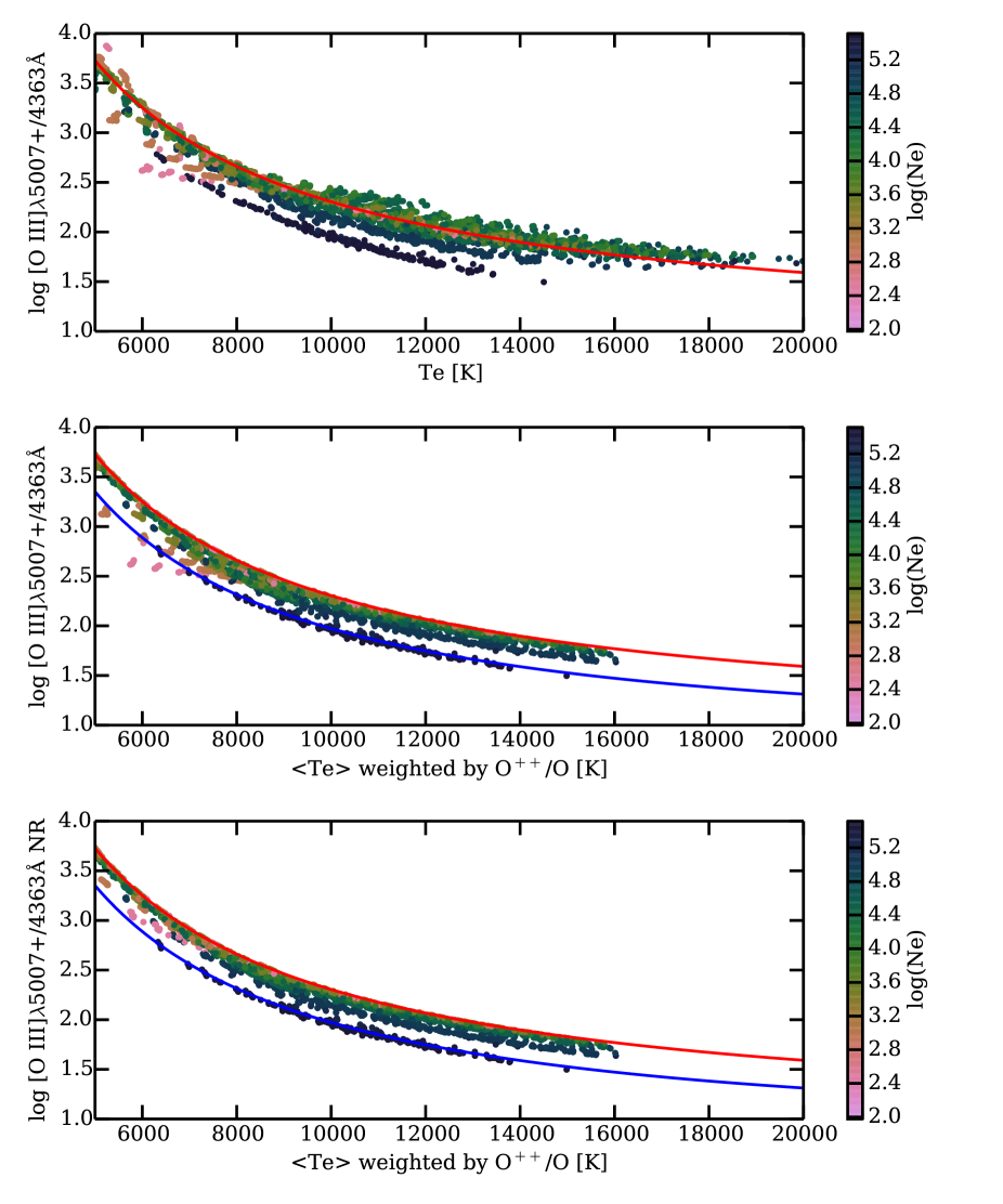
Figure 1: Temperature determined by $[{O\textsc{iii}}]\lambda$5007+4959/4363Å  line ratio (using PyNeb), vs. electron temperature. The color codes the electron density. Upper panel: the electron temperature is the mean over the whole nebula. Middle panel: the electron temperature is weighted by O⁺⁺/O, thus tracing the O⁺⁺ region. Lower panel: the $[{O\textsc{iii}}]\lambda$5007+4959/4363Å  line ratio is not taking into account the contribution of the recombination to $[{O\textsc{iii}}]\lambda$4363Å. The red (upper) and the blue (lower) lines are theoretical values, corresponding to the low density limit and to a density of $3.10^{5}$ cm^-3 respectively.

0.4.2 The effect of the ionization parameter on T_e([O iii])

In a recent paper, Nicholls et al. (2014) compare the distribution of the [O iii] electron temperature versus the oxygen gas-phase abundance observed in their sample of small isolated gas rich irregular dwarf galaxies (SIGRID). They find that classical simple photoionization models cannot well reproduce the observed behavior, in particular the high values of T([O iii]) obtained at low metallicity. The authors explore the different scenarios that can actually fit these extreme observations, and concluded that a combination of pressure and optical depths could readily explain them. We use here all the models from the 3MdB under the “HII_CHIm” reference (see 0.3.3 and Tab. 6) and plot in Fig. 2 the same quantities with the same axes ranges as in their Fig. 12. We find that we can reproduce all the observed points, once we take the ionization parameter log(U) as a free parameter. Using the relation log(U) $\propto Z^{-0.8}$ from Dopita et al. (2006b), normalized with log(U) = $-3$ at solar metallicity (i. e. 12 + log O/H = 8.69), we define a criterion to select the models so that log(U) = $3.93-0.8\times$(12 + log O/H), within a tolerance of 0.2 dex. This relation is similar to the one used by Pérez-Montero (2014). Those models are plotted in red in the same figure, and fit quite well the observed points from the SIGRID sample, even the extreme ones at low metallicity.

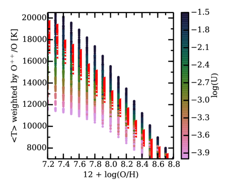
Figure 2: Electron temperature of the O⁺⁺ region vs. Oxygen abundance, colored by logU. The data are taken from the 3MdB “HII_CHIm” models. Red triangles (slightly x-shifted to be more visible) correspond to the models that fit the relation log(U) = $3.93-0.8\times$(12 + log O/H), within a tolerance of 0.2 dex.

0.4.3 When HOLMES ionize H ii regions

We use all the “DIG_HR” models (see Sec.0.3.1 and Table 4) to illustrate the effect of the hardening of the ionizing radiation on the emission line ratios [N ii]/H$\alpha$ and [O iii]/H$\beta$. This hardening occurs when the contribution of the HOLMES to the total ionizing SED increases. We show two emission-line ratio diagrams (commonly referred to as BPT after Baldwin et al., 1981). Fig. 3 shows [O iii]/H$\beta$ vs. [O ii]/H$\beta$ while Fig. 4 shows [O iii]/H$\beta$ vs. [N ii]/H$\alpha$ for different N/O abundance ratios. The colors code the contribution of the HOLMES to the total ionizing flux. The red and green contours contains half of the points for which this contribution is lower than 5% and greater than 90% respectively. They are obtained by estimating the probability density function (PDF) using a gaussian kernel density estimation.

In another example of the ionization of the interstellar gas by HOLMES, we use the “CALIFA” models (see Sec. 0.3.4) to plot [O iii]/H$\beta$ vs. [N ii]/H$\alpha$ for different ages and metallicities. In each subplot of Fig. 5, the grid is then scanning the effect of varying log(U) and N/O on the two line ratios [O iii]/H$\beta$ vs. [N ii]/H$\alpha$. From the left to the right, we see the effect of the metallicity and from top to bottom the effect of the age (only one of three ages is plotted here for concision).

We see that, for log(age) $\lesssim 6.7$, [O iii]/H$\beta$ globally decreases, as a consequence of the gradual disappearance of the most massive stars. The effect depends on metallicity. After log(age) $\gtrsim 8$, HOLMES take over the ionization (although at a much reduced pace, not perceptible in emission-line ratio diagrams but see Fig. 2 of Cid Fernandes et al., 2011). The values for [O iii]/H$\beta$ are higher in this phase than when ionization is due to O-B stars, because of the higher mean energy of the ionizing photons of the HOLMES (see Fig. 4 in Flores-Fajardo et al., 2011).

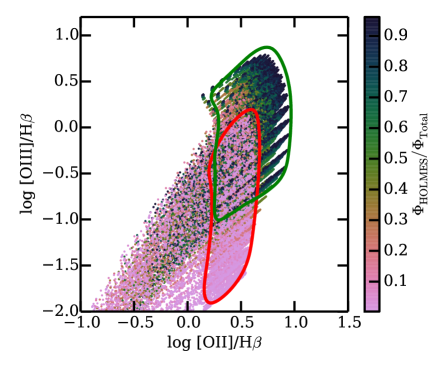
Figure 3: [O iii]/H$\beta$ vs. [O ii]/H$\beta$ for models referenced as “DIG_HR”. The red contour (the lower one) contains half of the points for which the contribution of the OB stars is greater than 95%. The green contour (the upper one) contains half of the points for which the contribution of the HOLMES is greater than 90%.

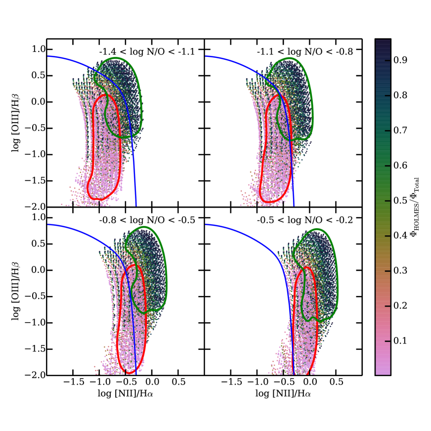
Figure 4: [O iii]/H$\beta$ vs. [N ii]/H$\beta$ for models referenced as “DIG_HR”, for various values of N/O. The blue line correspond to eq.  14 of Stasińska et al. (2006) dividing star forming galaxies and AGN hosts. Red and green countours have the same definition than in Fig. 3.

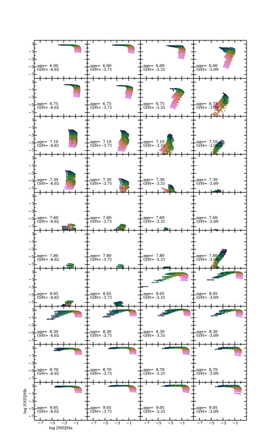
Figure 5: BPT diagrams for models referenced as “CALIFA”. In each panel we use 3 values for N/O, 5 values for the optical depth, 2 values for the geometry and 6 values for the ionization parameter log(U) (this latest being coded by the colors, from light pink corresponding to $-4$ to dark blue corresponding to $-1.5$). Panels from left to right shows the effect of varying the metallicity (of the ionizing SED and the gas) while panels from top to bottom shows the effect of varying the age of the ionizing population. The logarithms of the corresponding values are given in each panel.

0.4.4 Combined models of 2 densities

Most of the photoionization models found in the literature are 1D spherical or plane-parallel models. This is actually also the case for the 3MdB models. But if one needs to perform a tailored model to fit detailed and numerous observations of a given object, it often appears that more than one component is needed. It may be necessary to combine models of different optical depth (matter- and radiation-bounded models), models of different densities, models of different chemical compositions, and even any combination using this fundamental differences (e.g. Baldwin et al., 1995; Binette et al., 1996; Morisset & Pequignot, 1996; Morisset et al., 2002; Péquignot et al., 2003; Stasińska, 2005; Stasińska et al., 2010).

We can explore the properties of multi component models using models from the 3MdB, in particular we show here models where two regions of different densities are observed together. We extract models from the 3MdB under the reference “PNe_2014” (see Sec. 0.3.2 and Tab. 5), applying the following criteria: the ionizing source is a blackbody, the models are radiation-bounded, they have constant density and no dust, and they also fit the criteria described in Sec. 0.3.2 under the com6=1 condition to represent realistic planetary nebulae. From these models, we select only the ones with lowest hydrogen densities (100, 300 and 1000 cm^-3), that is 588 models. For each of these models, we look for models corresponding to the same ionizing star and the same chemical composition, but with the highest densities ($3.10^{4},10^{5}$ and $3.10^{5}$ cm^-3). The mean ionization parameter may be different between the 2 regions (depending on the densities, and on where the clump is located with respect to the ionizing star). The total number of models for the clumps under these assumptions is 14620. The models that are obtained by combining the 3MdB models are not included in the 3MdB.

For each pair of models associating a low density and a high density model, we compute two combined models by adding the line emissivities, using a weight for each region so that the contribution of the dense region to the total H$\beta$ intensity is 5 and 15% respectively. In the following example, we only concentrate on the “apparent” electron temperature, as determined from line ratios of classical $[{O\textsc{iii}}]\lambda$4363/5007Å and [N ii]$\lambda$5755/6584Å diagnostics, but any emission line can be computed using the same rule. We use the PyNeb package (Luridiana et al., 2014) to derive the temperatures from the line ratios of the original and combined models. In Fig. 6, we plot the electron temperatures as determined by the [N ii] line ratio vs. the one obtained from the [O iii] line ratio. The density used to determine both temperatures is the one obtained from the $[{S\textsc{ii}}]\lambda$6731/16Å line ratio. We plot in blue the values obtained for the low density medium alone, and in light green the ones obtained for the combined models. We can see that the values corresponding to the low density medium alone are close to the T([O iii]) = T([N ii]) red line. The marginal differences at high temperatures come from the temperature structure of the nebulae, leading to lower temperatures for the outer part of the nebula (the N⁺ region) compared to the more central part (the O⁺⁺ region). See also Sec. 0.4.5 on this topic. The effect of the high density clumps is to artificially increase the apparent [N ii] temperature. This is due to the fact that the critical density of the level 4 of N⁺ is $\sim 10^{5}$cm^-3, while the corresponding critical density for the O⁺⁺ ion is $\sim 7.10^{5}$cm^-3 (level 5 critical densities being of order of $10^{7}$cm^-3). The $[{N\textsc{ii}}]\lambda$6584Å emissivity is thus strongly reduced relative to the $[{N\textsc{ii}}]\lambda$5755Å one in clumps of density of order of $10^{5}$cm^-3, leading to a higher value of T([N ii]).

High T([N ii])/T([O iii]) are observed in high excitation planetary nebulae with Wolf-Rayet central stars (Peña et al., 2001; García-Rojas et al., 2012) and no satisfying explanation was given for that so far. The inclusion of dense clumps such as illustrated above might be the answer.

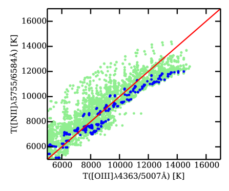
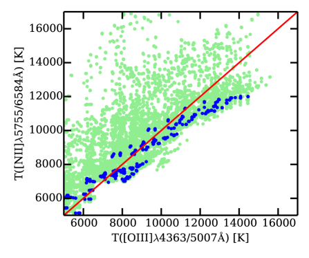
Figure 6: Apparent electron temperatures determined by the $[{N\textsc{ii}}]\lambda$5755/6584Å and the $[{O\textsc{iii}}]\lambda$4363/5007Å line ratios. The dark blue dots are single component low density models, the light green dots are combined models with 5 and 15% of H$\beta$ comming from dense clumps (upper and lower panel resp.). The red line follows the y=x relation.

0.4.5 Temperatures of the N⁺ and the O⁺⁺ regions in the different projects

One of the major advantage of the 3MdB is that all the models of the different projects are in a universal environment, allowing easy comparison. In this example, we plot in Fig. 7 the mean electron temperature weighted by the O⁺⁺/O ionic fraction versus the one weighted by N⁺/N. The plots are done separately for the four projects currently in the 3MdB. In all cases, we filter the models to only plot the ones that have $[{O\textsc{iii}}]\lambda$5007/H$\beta>0.05$ and $[{N\textsc{ii}}]\lambda$6584/H$\beta>0.05$, to avoid models where the O⁺⁺ or the N⁺ regions would be too small. In the case of the “PNe_2014” models, we filter the models with the com6 = 1 condition (the realistic models, see Sec.0.3.2). The blue line follows y=x, while the red line is following the relation $y=0.7\times x+3000$ from Campbell et al. (1986). Some trends are clearly seen:

• All the models are showing the expected trend of both temperatures increasing together.

• Neither of the two lines is a good fit to the points from the models, a somewhat large scatter is observed.

• In the case of “HII_CHIm” models, only one SED has been used and the departure from the y=x line is increasing with the ionization parameter.

• In the case of “DIG_HR” models, the ionization parameter is only scanning one order of magnitude (from $-4$ to $-3$), and the departure from the y=x is mainly due to the shape of the SED, changing from dominated by OB stars to dominated by HOLMES (not shown in this plots).

• In the cases of “PNe_2014” and “CALIFA” models, the SED and log(U) are changed and the result is a larger scatter around the y=x line, without a clear effect of log(U) alone.

• In all the cases, we do not see very high values of ${<T>}_{N^{+}/N}/{<T>}_{O^{++}/O}$ at ${<T>}_{O^{++}/O}$ larger than 10,000 K. The observed high values for this ratio in some planetary nebulae in this temperature range may be explained by the presence of high density clumps, see Sec. 0.4.4.

As an example of the use of MySQL to request data from the 3MdB, the following is the request for the lowest-right panel:

SELECT T_NITROGEN_vol_1, T_OXYGEN_vol_2,

logU_mean, O__3__5007A, TOTL__4861A,

N__2__6584A FROM tab, teion WHERE

(tab.ref = ’HII_CHIm’ and

O__3__5007A/H__1__4861A > 0.05 and

N__2__6584A/H__1__4861A > 0.05 and

tab.N = teion.N );

Notice the use of the field “N” to join the tables “tab” and “teion”. In the case of the “PNe_2014” models, a condition com6 = 1 has been added. The request results weight 6.1Mo, 441Ko, 957Ko, and 2.7Mo for ref = “PNe_2014”, “HII_CHIm”, “CALIFA”, and “DIG_HR” respectively.

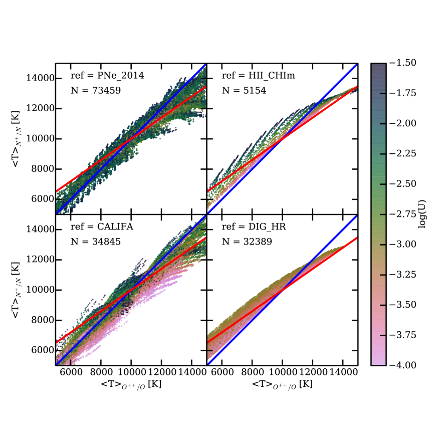
Figure 7: Mean electron temperature weighted by the O⁺⁺/O ionic fraction versus weighted by N⁺/N, for the four projects held in the 3MdB. The colors code the ionization parameter log(U) in the same way in every panel. The blue line shows the equal temperatures location. In the upper-left part of each panel the reference of the project and the number of points plotted are given. See text for more details on the filters applied to the models before plotting them. The blue line follows y=x, while the red line is following the relation $y=0.7\times x+3000$ from Campbell et al. (1986) .

0.5 Conclusions

We have presented in this paper the 3MdB, a new tool in the form of a database, to deal with grids of photoionization models. This tool is accessible with the MySQL protocol through Internet. It holds hundreds of thousands of photoionization models computed with the CLOUDY program (Ferland et al., 2013). For each model, more than 2600 parameters and model outputs are available. The power of the MySQL system allows the user to make complex requests based on filters to obtain subsets of this huge amount of data, in a format easy to read (e. g. coma-separated-variable ascii format). The 3MdB system currently holds 4 different projects (sets of data), other projects are planned to be incorporated in a near future. Up-to-date information is available from the 3MdB web page (https://sites.google.com/site/mexicanmillionmodels/).

We have shown with a few examples that the database can provide a very user-friendly way to study some aspects of the physics of the interstellar medium. Those examples are only illustrative, some of them will be developed in forthcoming papers.

It is worth noticing that the user is in fine responsible of the coherence of the work he is doing with the data extracted from the 3MdB. In particular, some care must be taken when comparing models computed with different versions of CLOUDY, or when dealing with models from the border of a grid, where the set of parameters may define irrealistic nebulae. In any case, for each particular project, the user should carefully check the relevance of the parameter space explored with the 3MdB subgrid used. The user needs to keep in mind that the models held in 3MdB suffer the limitations inherent to any photoionization model made with CLOUDY or with any other code: uncertainties in the atomic data or in the ionizing spectral energy distribution obtained from atmosphere models, optical properties of dust, among others.

The 3MdB is of public access through the MySQL protocol. The data are under the BSD-new license. For security reasons, the server IP, username and password for the direct access to the MySQL server are now only provided after asking by email to the authors. A user-web interface will be given as soon as possible, with full open access to the database.

One of the future extensions of the 3MdB is to be included as a Virtual Observatory service. This will provide more interfaces for the user to access the data.

Colleagues interested to include their grids of photoionization models in the 3MdB (because they do not have the computational ressources to run a large amount of models, to ease the accessibility to their results, or to insure the sustainability of their grid) are welcome to contact CM.

0.6 Acknowledgments

CM, GDI and NFF acknowledge support from the mexican project CONACyT CB-2010/153985. GDI gratefully aknowledges the DGAPA postdoctoral grant from the Universidad Nacional Autónoma de México. Many thanks to Grażyna Stasińska who kindly read and improved the manuscript. The authors gratefully acknowledge the constructive comments from the referee.

References

- Baldwin et al. (1995) Baldwin, J., Ferland, G., Korista, K., & Verner, D. 1995, ApJ, 455, L119
- Baldwin et al. (1981) Baldwin, J. A., Phillips, M. M., & Terlevich, R. 1981, PASP, 93, 5
- Barlow (1987) Barlow, M. J. 1987, MNRAS, 227, 161
- Binette et al. (1996) Binette, L., Wilson, A. S., & Storchi-Bergmann, T. 1996, A&A, 312, 365
- Bloecker (1995) Bloecker, T. 1995, A&A, 299, 755
- Campbell et al. (1986) Campbell, A., Terlevich, R., & Melnick, J. 1986, MNRAS, 223, 811
- Charlot & Longhetti (2001) Charlot, S. & Longhetti, M. 2001, MNRAS, 323, 887
- Cid Fernandes et al. (2014) Cid Fernandes, R., González Delgado, R. M., García Benito, R., Pérez, E., de Amorim, A. L., Sánchez, S. F., Husemann, B., Falcón Barroso, J., López-Fernández, R., Sánchez-Blázquez, P., Vale Asari, N., Vazdekis, A., Walcher, C. J., & Mast, D. 2014, A&A, 561, A130
- Cid Fernandes et al. (2013) Cid Fernandes, R., Pérez, E., García Benito, R., González Delgado, R. M., de Amorim, A. L., Sánchez, S. F., Husemann, B., Falcón Barroso, J., Sánchez-Blázquez, P., Walcher, C. J., & Mast, D. 2013, A&A, 557, A86
- Cid Fernandes et al. (2011) Cid Fernandes, R., Stasińska, G., Mateus, A., & Vale Asari, N. 2011, MNRAS, 413, 1687
- Delgado-Inglada et al. (2014) Delgado-Inglada, G., Morisset, C., & Stasińska, G. 2014, MNRAS, 440, 536
- Dopita et al. (2006a) Dopita, M. A., Fischera, J., Sutherland, R. S., Kewley, L. J., Leitherer, C., Tuffs, R. J., Popescu, C. C., van Breugel, W., & Groves, B. A. 2006a, ApJS, 167, 177
- Dopita et al. (2006b) Dopita, M. A., Fischera, J., Sutherland, R. S., Kewley, L. J., Tuffs, R. J., Popescu, C. C., van Breugel, W., Groves, B. A., & Leitherer, C. 2006b, ApJ, 647, 244
- Dopita et al. (2000) Dopita, M. A., Kewley, L. J., Heisler, C. A., & Sutherland, R. S. 2000, ApJ, 542, 224
- Dopita et al. (2013) Dopita, M. A., Sutherland, R. S., Nicholls, D. C., Kewley, L. J., & Vogt, F. P. A. 2013, ApJS, 208, 10
- Draine (2011) Draine, B. T. 2011, ApJ, 732, 100
- Ercolano et al. (2003) Ercolano, B., Barlow, M. J., Storey, P. J., & Liu, X. 2003, MNRAS, 340, 1136
- Ferland et al. (2013) Ferland, G. J., Porter, R. L., van Hoof, P. A. M., Williams, R. J. R., Abel, N. P., Lykins, M. L., Shaw, G., Henney, W. J., & Stancil, P. C. 2013, Rev. Mexicana Astron. Astrofis., 49, 137
- Fioc & Rocca-Volmerange (1997) Fioc, M. & Rocca-Volmerange, B. 1997, A&A, 326, 950
- Flores-Fajardo et al. (2011) Flores-Fajardo, N., Morisset, C., Stasińska, G., & Binette, L. 2011, MNRAS, 415, 2182
- García-Rojas et al. (2012) García-Rojas, J., Peña, M., Morisset, C., Mesa-Delgado, A., & Ruiz, M. T. 2012, A&A, 538, A54
- Gathier (1987) Gathier, R. 1987, A&AS, 71, 245
- Goodman et al. (2014) Goodman, A., Pepe, A., Blocker, A. W., Borgman, C. L., Cranmer, K., Crosas, M., Di Stefano, R., Gil, Y., Groth, P., Hedstrom, M., Hogg, D. W., Kashyap, V., Mahabal, A., Siemiginowska, A., & Slavkovic, A. 2014, PLoS Computational Biology, 10
- Groves et al. (2004) Groves, B. A., Dopita, M. A., & Sutherland, R. S. 2004, ApJS, 153, 75
- Kewley & Dopita (2002) Kewley, L. J. & Dopita, M. A. 2002, ApJS, 142, 35
- Kewley et al. (2001) Kewley, L. J., Dopita, M. A., Sutherland, R. S., Heisler, C. A., & Trevena, J. 2001, ApJ, 556, 121
- Korista et al. (1997) Korista, K., Baldwin, J., Ferland, G., & Verner, D. 1997, ApJS, 108, 401
- Leitherer et al. (1999) Leitherer, C., Schaerer, D., Goldader, J. D., González Delgado, R. M., Robert, C., Kune, D. F., de Mello, D. F., Devost, D., & Heckman, T. M. 1999, ApJS, 123, 3
- Levesque et al. (2010) Levesque, E. M., Kewley, L. J., & Larson, K. L. 2010, AJ, 139, 712
- Luridiana et al. (2014) Luridiana, V., Morisset, C., & Shaw, R. A. 2014, ArXiv e-prints
- Mollá et al. (2009) Mollá, M., García-Vargas, M. L., & Bressan, A. 2009, MNRAS, 398, 451
- Morisset (2013) Morisset, C. 2013, pyCloudy: Tools to manage astronomical Cloudy photoionization code
- Morisset (2014) Morisset, C. 2014, in Asymmetrical Planetary Nebulae VI conference, Proceedings of the conference held 4-8 November, 2013. Edited by C. Morisset, G. Delgado-Inglada and S. Torres-Peimbert.
- Morisset & Pequignot (1996) Morisset, C. & Pequignot, D. 1996, A&A, 312, 135
- Morisset et al. (2002) Morisset, C., Schaerer, D., Martín-Hernández, N. L., Peeters, E., Damour, F., Baluteau, J., Cox, P., & Roelfsema, P. 2002, A&A, 386, 558
- Nicholls et al. (2014) Nicholls, D. C., Dopita, M. A., Sutherland, R. S., Jerjen, H., & Kewley, L. J. 2014, ApJ, 790, 75
- Peña et al. (2001) Peña, M., Stasińska, G., & Medina, S. 2001, A&A, 367, 983
- Pepe et al. (2014) Pepe, A., Goodman, A., Muench, A., Crosas, M., & Erdmann, C. 2014, PLoS ONE, 9
- Péquignot et al. (2003) Péquignot, D., Liu, X., Barlow, M. J., Storey, P. J., & Morisset, C. 2003, in IAU Symposium, Vol. 209, Planetary Nebulae: Their Evolution and Role in the Universe, ed. S. Kwok, M. Dopita, & R. Sutherland, 347
- Pérez-Montero (2014) Pérez-Montero, E. 2014, MNRAS, 441, 2663
- Proxauf et al. (2014) Proxauf, B., Öttl, S., & Kimeswenger, S. 2014, A&A, 561, A10
- Rauch (1997) Rauch, T. 1997, A&A, 320, 237
- Rémy-Ruyer et al. (2014) Rémy-Ruyer, A., Madden, S. C., Galliano, F., Galametz, M., Takeuchi, T. T., Asano, R. S., Zhukovska, S., Lebouteiller, V., Cormier, D., Jones, A., Bocchio, M., Baes, M., Bendo, G. J., Boquien, M., Boselli, A., DeLooze, I., Doublier-Pritchard, V., Hughes, T., Karczewski, O. Ł., & Spinoglio, L. 2014, A&A, 563, A31
- Reynolds (1971) Reynolds, R. J. 1971, PhD thesis, THE UNIVERSITY OF WISCONSIN - MADISON.
- Reynolds (1991) Reynolds, R. J. 1991, in IAU Symposium, Vol. 144, The Interstellar Disk-Halo Connection in Galaxies, ed. H. Bloemen, 67–76
- Schoenberner (1983) Schoenberner, D. 1983, ApJ, 272, 708
- Stasińska (1980) Stasińska, G. 1980, A&A, 84, 320
- Stasińska (2005) —. 2005, A&A, 434, 507
- Stasińska et al. (2006) Stasińska, G., Cid Fernandes, R., Mateus, A., Sodré, L., & Asari, N. V. 2006, MNRAS, 371, 972
- Stasińska & Leitherer (1996) Stasińska, G. & Leitherer, C. 1996, ApJS, 107, 661
- Stasińska et al. (2010) Stasińska, G., Morisset, C., Tovmassian, G., Rauch, T., Richer, M. G., Peña, M., Szczerba, R., Decressin, T., Charbonnel, C., Yungelson, L., Napiwotzki, R., Simón-Díaz, S., & Jamet, L. 2010, A&A, 511, A44
- Stasińska et al. (1991) Stasińska, G., Tylenda, R., Acker, A., & Stenholm, B. 1991, A&A, 247, 173
- Sutherland & Dopita (1993) Sutherland, R. S. & Dopita, M. A. 1993, ApJS, 88, 253