Electron-positron pair creation in low-energy collisions of heavy bare nuclei

Abstract

A method for calculations of electron-positron pair-creation probabilities in low-energy heavy-ion collisions is developed. The approach is based on the propagation of all one-electron states via the numerical solving of the time-dependent Dirac equation in the monopole approximation. The electron wave functions are represented as finite sums of basis functions constructed from B-splines using the dual-kinetic-balance technique. The calculations of the created particle numbers and the positron energy spectra are performed for the collisions of bare nuclei at the energies near the Coulomb barrier with the Rutherford trajectory and for different values of the nuclear charge and the impact parameter. To examine the role of the spontaneous pair creation the collisions with a modified velocity and with a time delay are also considered. The obtained results are compared with the previous calculations and the possibility of observation of the spontaneous pair creation is discussed.

I INTRODUCTION

The stationary Dirac equation leads to a singularity in the solution for the ground state of an electron in the field of the pointlike nucleus with the charge $Z>$137. But for an extended nucleus the energy of the 1$s_{1/2}$ state $E(Z)$ goes continuously beyond the point $Z=137$ and reaches the negative-energy continuum at the critical value $Z_{\rm C}\approx 173$ Pomeranchuk_45 ; Gershtein_70 ; Greiner_69 ; Zeldovich_71 . As predicted independently by Gershtein and Zeldovich Gershtein_70 and by Pieper and Greiner Greiner_69 , if the empty level dives into the negative-energy continuum, then it turns into a resonance that can lead to the spontaneous decay of the vacuum via emission of a positron and occupation of the supercritical K-shell by an electron. The experimental observation of this effect would confirm the predictions of quantum electrodynamics in the highly nonperturbative supercritical domain. Unfortunately, the charge of the heaviest produced nuclei is far less than the required one, $Z_{\rm C}$. However, in the collision of two ions, if their total charge is sufficiently large, the ground state of the formed quasimolecular system can become so deeply bound that the spontaneous pair creation is possible. The most favorable collision energy for investigation of the supercritical regime is about the Coulomb barrier Greiner_85 . In heavy-ion collisions, the electron-positron pairs can also be created dynamically due to the time-dependent potential of the moving ions. In order to find the signal from the vacuum decay one needs to distinguish the spontaneously produced pairs from the dynamical background.

The experiments for searching the spontaneous pair creation were performed at GSI (Darmstadt, Germany) using the collisions of partially stripped ions with neutral atoms, but no evidence of the vacuum decay was found Muller_94 . It should be noticed that for studying this phenomenon the collisions of bare nuclei would be more favorable due to the empty K-shell. It is expected that the upcoming Facility for Antiproton and Ion Research (FAIR) will provide new opportunities for investigations of low-energy heavy-ion collisions, probably including the collisions of fully stripped ions fair_design_01 ; Gumbaridze_09 .

To date a number of approaches to calculations of various processes in low-energy heavy-ion collisions have been proposed Gershtein_73 ; Popov_73 ; Peitz_73 ; Reinhardt_81 ; Muller_88 ; Kurpick_92 ; Ackad_07 ; Ackad_08 ; Tup_10 ; Tup_12 ; Kozhedub_2013 ; Bondarev_2013 ; Maltsev_2013 ; Mac_12 ; Deyneka_13 ; Kozhedub_14 ; Khriplovich_14 . In Refs. Gershtein_73 ; Popov_73 ; Peitz_73 , the pair-creation process was considered in the static approximation, according to which the corresponding probability is proportional to the resonance width $\Gamma(R)$ which depends on the internuclear distance $R(t)$. Such an approximation does not take into account the dynamical effects. A more advanced approach was based on the propagation of a finite number of initial states using the time-dependent adiabatic basis set with the Feshbach projection technique (see Refs. Reinhardt_81 ; Greiner_85 ; Muller_88 and references therein). This method allowed calculations of the pair-creation probabilities employing small numbers of the basis functions. However, the small basis size might lead to the low resolution of the continuum. From the results, which were basically obtained in the monopole approximation, it was concluded that the spontaneous contribution is indistinguishable from the dynamical background in the positron spectra in elastic collisions, and only in hypothetical collisions with the nuclear sticking can there be the visible effects of the vacuum decay Reinhardt_81 ; Muller_88 . Another dynamical approach Ackad_07 ; Ackad_08 was based on solving the time-dependent Dirac equation in the monopole approximation with the mapped Fourier grid method. In Ref. Ackad_08 , the pair-creation probabilities were calculated with propagation of all initial states of a very large basis set, compared to the previous works, that might improve the energy resolution of the continuum. For the collisions of bare uranium nuclei, the results for the positron spectra were quite different from those in Ref. Muller_88 . The importance of the dynamical pair-production effects follows also from the recent perturbative evaluation of Ref. Khriplovich_14 .

In the present work, we develop an alternative method for calculations of the pair-creation probabilities in low-energy heavy-ion collisions. In this method, the time-dependent Dirac equation is solved numerically in the monopole approximation employing the stationary basis set. The basis functions are constructed from the B-splines using the dual-kinetic-balance (DKB) approach Shabaev:prl:04 , which prevents the appearance of nonphysical spurious states. The DKB B-spline basis set provides a very accurate representation of the continuum and previously was successfully used in QED calculations for the summation over the whole Dirac spectrum (see, e.g., Refs. Shabaev_05 ; Kozhedub_10 ). All of the eigenvectors of the initial Hamiltonian matrix are propagated in order to obtain the one-electron transition amplitudes, which are used to calculate the particle-production probabilities. The calculations are performed for the symmetric collisions of bare nuclei with different values of the nuclear charge at the energy near the Coulomb barrier.

The paper is organized as follows. The pair-creation process in a time-dependent external field is briefly discussed in Sec. II.1. The monopole approximation is considered in Sec. II.2. The method for solving the time-dependent Dirac equation is described in Sec. II.3. The obtained results and their comparison with the previous calculations are presented in Sec. III.

The relativistic units ($\hbar=c=1$) are used throughout the paper.

II THEORY

II.1 Pair creation in external field

In the present work we take into account the interaction of electrons with the strong external field nonperturbatively, but neglect the electron-electron interaction, assuming the electrons can influence each other only via the Pauli exclusion principle. The positron states as well as the creation of electron-positron pairs can be treated within the Dirac original model where the negative-energy states are considered to be initially occupied by electrons. The production of an electron-positron pair appears as a transition of an electron from the negative-energy continuum to a positive-energy state, in formal agreement with quantum electrodynamics. The negative-energy electron states properly transformed describe the states of positrons, which in the mentioned model correspond to the holes in the filled lower continuum.

The one-electron dynamics is determined by the time-dependent Dirac equation

$$i\frac{\partial\psi({\mbox{\boldmath$r$}},t)}{\partial t}=\hat{H}_{D}(t)\,\psi({\mbox{\boldmath$r$}},t)\,,$$ (1)

where

$$\hat{H}_{D}(t)={\mbox{\boldmath$\alpha$}}\left({\mbox{\boldmath$p$}}-e{\mbox{\boldmath$A$}}(t)\right)+V(t)+m_{e}\beta$$ (2)

and the potential $(V(t),{\mbox{\boldmath$A$}}(t))$ describes the interaction with the external field. One can define the solutions $\psi^{(+)}_{i}({\mbox{\boldmath$r$}},t)$ and $\psi^{(-)}_{i}({\mbox{\boldmath$r$}},t)$ of Eq. (1) with the following boundary conditions

$$\psi^{(+)}_{i}({\mbox{\boldmath$r$}},t_{\rm in})=\varphi^{\rm in}_{i}({\mbox{\boldmath$r$}}),\,\psi^{(-)}_{i}({\mbox{\boldmath$r$}},t_{\rm out})=\varphi^{\rm out}_{i}({\mbox{\boldmath$r$}}),$$ (3)

$$\hat{H}_{D}(t_{\rm in})\,\varphi^{\rm in}_{i}({\mbox{\boldmath$r$}})=\varepsilon^{\rm in}_{i}\varphi^{\rm in}_{i}({\mbox{\boldmath$r$}}),\,\hat{H}_{D}(t_{\rm out})\,\varphi^{\rm out}_{i}({\mbox{\boldmath$r$}})=\varepsilon^{\rm out}_{i}\varphi^{\rm out}_{i}({\mbox{\boldmath$r$}}),$$ (4)

where $t_{\rm in}$ is the initial and $t_{\rm out}$ is the final time moment. In the final expressions it will be assumed that $t_{\rm in}\rightarrow-\infty$ and $t_{\rm out}\rightarrow\infty$.

The formulas for the probabilities of pair creation can be derived using the second quantization technique Greiner_85 ; Fradkin_91 . In the Heisenberg picture, one can introduce the time-dependent field operator $\hat{\Psi}({\mbox{\boldmath$r$}},t)$ and the time-independent state vectors $\arrowvert 0,\rm in\rangle$ and $\arrowvert 0,\rm out\rangle$, which correspond to the fully occupied negative-energy continua at $t_{\rm in}$ and $t_{\rm out}$, respectively. Using the functions $\psi_{i}^{(+)}({\mbox{\boldmath$r$}},t)$ and $\psi_{i}^{(-)}({\mbox{\boldmath$r$}},t)$, the operator $\hat{\Psi}({\mbox{\boldmath$r$}},t)$ can be expanded as

$$\hat{\Psi}({\mbox{\boldmath$r$}},t)=\sum_{i>F}\hat{b}^{\rm(in)}_{i}\,\psi^{(+)}_{i}({\mbox{\boldmath$r$}},t)+\sum_{i<F}\hat{d}^{\rm\,(in)\,\dagger}_{i}\,\psi^{(+)}_{i}({\mbox{\boldmath$r$}},t),$$ (5)

$$\hat{\Psi}({\mbox{\boldmath$r$}},t)=\sum_{i>F}\hat{b}^{\rm(out)}_{i}\,\psi^{(-)}_{i}({\mbox{\boldmath$r$}},t)+\sum_{i<F}\hat{d}^{\rm\,(out)\,\dagger}_{i}\,\psi^{(-)}_{i}({\mbox{\boldmath$r$}},t).$$ (6)

Here the Fermi level $F$ is the border between the filled negative-energy states and the vacant positive-energy states ($\varepsilon_{F}=-m_{e}$), $\hat{b}^{\rm(in)}_{i}$ and $\hat{b}^{\rm(out)}_{i}$ are the annihilation operators for electrons, and $\hat{d}^{\rm\,(in)\,\dagger}_{i}$ and $\hat{d}^{\rm\,(out)\,\dagger}_{i}$ are the creation operators for holes (positrons). They obey the standard anticommutation relations and their action on the vacuum states is

$$\hat{b}_{i}^{\rm(in)}\arrowvert 0,{\rm in}\rangle=0,\quad\hat{b}_{i}^{\rm(out)}\arrowvert 0,{\rm out}\rangle=0\quad{\rm for}\,\,i>F$$ (7)

and

$$\hat{d}_{i}^{\rm\,(in)}\arrowvert 0,{\rm in}\rangle=0,\quad\hat{d}_{i}^{\rm\,(out)}\arrowvert 0,{\rm out}\rangle=0\quad{\rm for}\,\,i<F.$$ (8)

It should be noted that these operators refer to the physical particles only at the corresponding time moments $t_{\rm in}$ and $t_{\rm out}$.

Since we assume that at the initial time moment $t_{\rm in}$, the negative-energy continuum is occupied and all of the positive-energy states are free, the system is described by the vector $\arrowvert 0,\rm{in}\rangle$. The operators should correspond to the particles produced at $t_{\rm out}$, which is the measurement time. By employing Eqs. (5), and (6), and the anticommutation relations between the annihilation and creation operators, one can derive the following expressions for the numbers of electrons $n_{k}$ and positrons $\overline{n}_{p}$ created in the states $k>F$ and $p<F$, respectively Greiner_85 ; Fradkin_91 :

$$n_{k}=\langle 0,{\rm in}\lvert\hat{b}^{\rm(out)\,\dagger}_{k}\hat{b}^{\rm(out)}_{k}\rvert 0,{\rm in}\rangle=\sum_{i<F}\arrowvert a_{ik}\arrowvert^{2}\,,$$ (9)

$$\overline{n}_{p}=\langle 0,{\rm in}\lvert\hat{d}^{\rm\,(out)\,\dagger}_{p}\hat{d}^{\rm\,(out)}_{p}\rvert 0,{\rm in}\rangle=\sum_{i>F}\arrowvert a_{ip}\arrowvert^{2}\,,$$ (10)

where

$$a_{ij}(t)=\int d^{3}{\mbox{\boldmath$r$}}\,\psi^{(-)\dagger}_{i}({\mbox{\boldmath$r$}},t)\,\psi^{(+)}_{j}({\mbox{\boldmath$r$}},t)=a_{ij}$$ (11)

are the one-electron transition amplitudes, which are time independent because the functions $\psi_{i}^{(+)}({\mbox{\boldmath$r$}},t)$ and $\psi_{i}^{(-)}({\mbox{\boldmath$r$}},t)$ are solutions of Eq. (1). For calculation of $n_{k}$ and $\overline{n}_{p}$, we use the finite-basis-set method and, therefore, in Eqs. (9) and (10) the summation runs over a finite number of states. In order to obtain $a_{ij}$, the eigenstates $\varphi^{\rm in}_{i}({\mbox{\boldmath$r$}})$ of the initial Hamiltonian $\hat{H}(t_{\rm in})$, including the bound states and the states of the both discretized continua, are evolved to the time $t_{\rm out}$ via solving the time-dependent Dirac equation and are then projected on the eigenstates $\varphi^{\rm out}_{j}({\mbox{\boldmath$r$}})$ of the final Hamiltonian $\hat{H}(t_{\rm out})$:

$$a_{ij}=\int d^{3}{\mbox{\boldmath$r$}}\,\varphi^{(\rm out)\dagger}_{i}({\mbox{\boldmath$r$}})\,\psi^{(+)}_{j}({\mbox{\boldmath$r$}},t_{\rm out}).$$ (12)

The total number of created particles is given by

$$P=\sum_{k>F}\,n_{k}=\sum_{p<F}\,\overline{n}_{p}.$$ (13)

In the discrete basis set, the positron energy spectrum can be calculated using the Stieltjes method Langhoff_74 :

$$\frac{dP}{dE}\left(\frac{\varepsilon^{\rm out}_{p}+\varepsilon^{\rm out}_{p+1}}{2}\right)=\frac{1}{2}\frac{\overline{n}_{p+1}+\overline{n}_{p}}{\varepsilon^{\rm out}_{p+1}-\varepsilon^{\rm out}_{p}}.$$ (14)

II.2 Monopole approximation

We consider the low-energy collision of two heavy bare nuclei $A$ and $B$ which move along the classical trajectories. In the field of the nuclei, the electron dynamics is described by Eq. (1) with the two-center potential,

$$V({\mbox{\boldmath$r$}},t)=V^{A}_{\rm nucl}\left({\mbox{\boldmath$r$}}-{\mbox{\boldmath$R$}}_{A}(t)\right)+V^{B}_{\rm nucl}\left({\mbox{\boldmath$r$}}-{\mbox{\boldmath$R$}}_{B}(t)\right)\,,$$ (15)

where ${\mbox{\boldmath$R$}}_{A}$ and ${\mbox{\boldmath$R$}}_{B}$ denote the nuclear positions and

$$V_{\rm nucl}({\mbox{\boldmath$r$}})=\int d^{3}{\mbox{\boldmath$r$}}^{\prime}\frac{\rho_{\rm nucl}\left({\mbox{\boldmath$r$}}^{\prime}\right)}{\lvert{\mbox{\boldmath$r$}}-{\mbox{\boldmath$r$}}^{\prime}\rvert}.$$ (16)

In this paper, we use the uniformly charged sphere model for the nuclear charge-density distribution $\rho_{\rm nucl}({\mbox{\boldmath$r$}})$. The vector potential $A$ can be neglected due to the low collision energy.

The numerical solving of the time-dependent Dirac equation with the two-center potential (15) requires very demanding three-dimensional calculations. One may expect, however, that the main contribution to the pair creation results from the short internuclear distances, where the symmetric quasimolecular system is well described within the monopole approximation Reinhardt_81 . In this approximation, only the spherically symmetric part of the partial expansion of the potential (15) is taken into account:

$$V_{\rm mon}(r,t)=\frac{1}{4\pi}\int d\Omega\,V({\mbox{\boldmath$r$}},t)\,.$$ (17)

Here we assume that the origin of the coordinate frame is chosen at the center of mass. For the central field (17) the Dirac wave function can be written as

$$\psi_{\kappa m}({\mbox{\boldmath$r$}},t)=\left(\begin{array}[]{l}\displaystyle\,\,\frac{~{}G_{\kappa}(r,t)}{r}\,\chi_{\kappa m}(\Omega)\\[11.38109pt] \displaystyle i\,\frac{F_{\kappa}(r,t)}{r}\,\chi_{-\kappa m}(\Omega)\end{array}\right)\,,$$ (18)

where $G_{\kappa}(r,t)$ and $F_{\kappa}(r,t)$ are the large and small radial components, respectively, $\chi_{\kappa m}(\Omega)$ is the spherical spinor, and $\kappa=(-1)^{j+l+1/2}(j+1/2)$ is the relativistic angular quantum number. Substituting the expression (18) into the Dirac Eq. (1) leads to

$$i\frac{\partial}{\partial t}\phi(r,t)=\hat{H}(t)\,\phi(r,t)\,,$$ (19)

where

$$\phi(r,t)=\left(\begin{array}[]{lll}G(r,t)\\ F(r,t)\end{array}\right)$$ (20)

and

$$\hat{H}(t)=\left(\begin{array}[]{cc}\displaystyle V_{\rm mon}(r,t)+m_{e}&\displaystyle-\frac{d}{dr}+\frac{\kappa}{r}\\[11.38109pt] \displaystyle\frac{d}{dr}+\frac{\kappa}{r}&\displaystyle V_{\rm mon}(r,t)-m_{e}\end{array}\right)$$ (21)

is the radial Dirac Hamiltonian.

For large nuclear separation, the one-electron energy levels of the monopole Hamiltonian $\hat{H}(t)$ are quite different from the real two-center ones. However, the vacuum state defined with respect to the instantaneous monopole Hamiltonian at some large internuclear distance can be considered as the initial state of the system since, as assumed above, the particles are mainly produced at short internuclear distances, where the monopole approximation is valid. The limitation of the employed model is that we can not isolate the final population of a particular one-electron state belonging to one of the nuclei.

II.3 Dirac equation in a finite basis set

For solving Eq. (19), we employ the time-independent finite basis set $\{u_{k}(r)\}$:

$$\phi(r,t)=C_{k}(t)\,u_{k}(r)\,,$$ (22)

$$iS_{jk}\,\frac{dC_{k}(t)}{dt}=H_{jk}(t)C_{k}(t)\,,$$ (23)

where $S_{jk}=\langle u_{j}\arrowvert u_{k}\rangle$, $H_{jk}(t)=\langle u_{j}\arrowvert\hat{H}(t)\arrowvert u_{k}\rangle$, and the Hamiltonian $\hat{H}(t)$ is defined by Eq. (21). Here and below, the summation over the repeated indices is implied. Equation (23) is solved using the Crank-Nicolson method Crank_47 . According to this method, for a short time interval $\Delta t$, the coefficients $C_{k}(t+\Delta t)$ can be found from the system of linear equations

$$\left[S_{jk}\,+\frac{i\Delta t}{2}\,\,H_{jk}(t+\Delta t/2)\,\right]\,C_{k}(t+\Delta t)\,=\,\left[S_{jk}-\frac{i\Delta t}{2}\,H_{jk}(t+\Delta t/2)\right]\,C_{k}(t).$$ (24)

We solve the system (24) employing the iterative BiCGS (BiConjugate Gradient Squared) algorithm Joly_93 . It should be noted that the Crank-Nicolson method conserves the norm of the wave function at each time step Deyneka_13 .

In order to obtain the initial states, one can start from the variational principle

$$\delta\mathcal{F}=0\,,$$ (25)

$$\mathcal{F}=\langle\phi\lvert(\hat{H}_{0}-\varepsilon)\rvert\phi\rangle\,,$$ (26)

which is equivalent to the stationary Dirac equation. The Lagrange multiplier $\varepsilon$ corresponds to the energy of an eigenstate of the instantaneous Hamiltonian $\hat{H}_{0}=\hat{H}(t_{\rm in})$ at the initial time moment $t_{\rm in}$. Substituting the expansion (22) into Eq. (25), one gets the system of equations

$$\frac{d\mathcal{F}}{dC_{k}}=0\,.$$ (27)

This system leads to the generalized eigenvalue problem

$$H_{jk}C_{k}=\varepsilon S_{jk}C_{k}\,,$$ (28)

which can be solved using the standard numerical routines.

A disadvantage of the straightforward implementation of the finite-basis-set method is the presence of nonphysical spurious states for $\kappa>0$. To avoid such states, we employ the DKB approach Shabaev:prl:04 . According to this approach, the basis functions are constructed as

$$u_{k}(r)=\left(\begin{array}[]{c}\displaystyle\pi_{k}(r)\\[11.38109pt] \displaystyle\frac{1}{2m_{e}}\left(\frac{d}{dr}+\frac{\kappa}{r}\right)\pi_{k}(r)\end{array}\right),\qquad k\leq n\,,$$ (29)

$$u_{k}(r)=\left(\begin{array}[]{c}\displaystyle\frac{1}{2m_{e}}\left(\frac{d}{dr}-\frac{\kappa}{r}\right)\pi_{k-n}(r)\\[11.38109pt] \displaystyle\pi_{k-n}(r)\end{array}\right),\qquad k>n\,,$$ (30)

where $2n$ is the size of the basis set and $\pi_{k}$ are linear-independent functions which are assumed to be square integrable and satisfy the proper boundary conditions. In the present work, we have chosen B-splines as $\pi_{k}$. The B-splines of any degree can be easily constructed using the recursive algorithm De_Boor_01 ; Johnson_88 . With this basis, the Hamiltonian and overlapping matrices are sparse, which facilitates the numerical calculations.

III RESULTS

In this section, we present the results of our calculations of the pair-creation probabilities in the collisions of two identical bare nuclei at the energy near the Coulomb barrier. Unless stated otherwise, the nuclei are assumed to move along the classical Rutherford trajectories. The nuclear charge distribution is given by a uniformly charged sphere of radius $R_{\rm n}=1.2\times A^{1/3}$ fm, where $A$ is the atomic mass number. The calculations were performed employing the method described in Sec. II for the states with the relativistic quantum number $\kappa=-1$ and $\kappa=1$. There is no coupling between these sets in the monopole approximation and they are expected to give the dominant contribution to the pair creation Reinhardt_81 . We used 410 basis functions constructed from B-splines of ninth order defined in a box of size $L=10^{5}$ fm. The B-spline knots were distributed exponentially in order to better describe the wave functions in the region of the closest approach of the nuclei. It was found that this basis set is sufficient to obtain the convergent results. All of the initial states, including 10 bound, 195 positive-continuum, and 205 negative-continuum ones, were propagated in order to obtain the one-electron transition amplitudes. The particle numbers were calculated according to the formulas (9) and (10) for a fixed projection $m$ of the total angular momentum $j=1/2$ and were then doubled in order to take into account the contributions of channels with both values of $m$.

In Fig. 1, we present the obtained positron energy spectra for the U$-$U collision for the different values of the impact parameter $b$ at kinetic energy $E_{\rm cm}=$740 MeV in the center-of-mass frame.

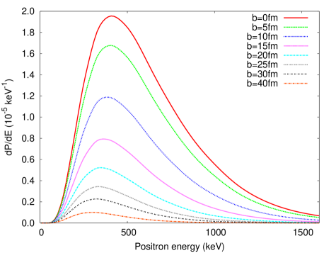
Figure 1: (Color online) Positron energy spectrum for the U$-$U collision at energy $E_{\rm cm}=$740 MeV for the different values of the impact parameter $b$.

These results are very similar to those presented in Ref. Muller_88 . The collisions with $b=30$ fm and $b=40$ fm are subcritical, and with $b\leq 25$ fm, they are supercritical. However, the calculated positron spectra do not exhibit any qualitative difference between the subcritical and supercritical regimes.

In Table 1, the obtained numbers of created pairs for the U$-$U collision at $E_{\rm cm}=740$ MeV and $E_{\rm cm}=680$ MeV are presented and compared with the corresponding values from Ref. Muller_88 . The results are in good agreement with each other, but in our case the contribution of pairs with a free electron is relatively larger. This can be due to a more dense representation of the continuum states in our calculations. Nevertheless, as one can see from Table 1, the created electrons are mainly captured into the bound states.

Table 1: Number of created pairs in the U$-$U collision at energy $E_{\rm cm}$ as a function of the impact parameter $b$. $P_{t}$ is the total number of pairs and $P_{b}$ is the number of pairs with an electron captured into a bound state.

		Müller et al. Muller_88		This work
$E_{\rm cm}$ (MeV)	$b$ (fm)	$P_{\tiny b}$	$P_{t}$	$P_{b}$	$P_{t}$
740	0	1.23 $\times$ $10^{-2}$	1.26 $\times$ $10^{-2}$	1.25 $\times$ $10^{-2}$	1.29 $\times$ $10^{-2}$
	5	1.04 $\times$ $10^{-2}$	1.06 $\times$ $10^{-2}$	1.05 $\times$ $10^{-2}$	1.08 $\times$ $10^{-2}$
	10	7.04 $\times$ $10^{-3}$	7.15 $\times$ $10^{-3}$	7.03 $\times$ $10^{-3}$	7.26 $\times$ $10^{-3}$
	15	4.41 $\times$ $10^{-3}$	4.47 $\times$ $10^{-3}$	4.39 $\times$ $10^{-3}$	4.51 $\times$ $10^{-3}$
	20	2.71 $\times$ $10^{-3}$	2.73 $\times$ $10^{-3}$	2.70 $\times$ $10^{-3}$	2.75 $\times$ $10^{-3}$
	25	1.67 $\times$ $10^{-3}$	1.68 $\times$ $10^{-3}$	1.66 $\times$ $10^{-3}$	1.69 $\times$ $10^{-3}$
	30	1.04 $\times$ $10^{-3}$	1.04 $\times$ $10^{-3}$	1.03 $\times$ $10^{-3}$	1.04 $\times$ $10^{-3}$
	40	4.11 $\times$ $10^{-4}$	4.11 $\times$ $10^{-4}$	4.09 $\times$ $10^{-4}$	4.12 $\times$ $10^{-4}$
680	0	1.04 $\times$ $10^{-2}$	1.06 $\times$ $10^{-2}$	1.05 $\times$ $10^{-2}$	1.07 $\times$ $10^{-2}$
	5	8.86 $\times$ $10^{-3}$	8.97 $\times$ $10^{-3}$	8.87 $\times$ $10^{-3}$	9.10 $\times$ $10^{-3}$
	10	6.05 $\times$ $10^{-3}$	6.12 $\times$ $10^{-3}$	6.03 $\times$ $10^{-3}$	6.17 $\times$ $10^{-3}$
	15	3.80 $\times$ $10^{-3}$	3.83 $\times$ $10^{-3}$	3.78 $\times$ $10^{-3}$	3.85 $\times$ $10^{-3}$
	20	2.33 $\times$ $10^{-3}$	2.34 $\times$ $10^{-3}$	2.32 $\times$ $10^{-3}$	2.35 $\times$ $10^{-3}$
	25	1.43 $\times$ $10^{-3}$	1.43 $\times$ $10^{-3}$	1.42 $\times$ $10^{-3}$	1.44 $\times$ $10^{-3}$
	30	8.80 $\times$ $10^{-4}$	8.80 $\times$ $10^{-4}$	8.75 $\times$ $10^{-4}$	8.82 $\times$ $10^{-4}$
	40	3.42 $\times$ $10^{-4}$	3.42 $\times$ $10^{-4}$	3.41 $\times$ $10^{-4}$	3.43 $\times$ $10^{-4}$

In order to study possible evidences of the spontaneous pair creation, we considered the collisions of nuclei with different charge $Z$. Figure 2 shows the obtained positron spectra for the Fr$-$Fr ($Z$=87), U$-$U ($Z$=92), and Db$-$Db ($Z$=105) head-on collisions at $E_{\rm cm}=674.5$, $E_{\rm cm}=740$, and $E_{\rm cm}=928.4$ MeV, respectively. For these energies, the minimal distance between the nuclear surfaces is the same for all three cases (about $1.6$ fm). The Fr$-$Fr collision is subcritical and has the purely dynamical positron spectrum. In the Db$-$Db collision, one can expect an enhancement of the spontaneous pair creation due to the deep supercritical resonance Ackad_08 . However, all three curves in Fig. 2 have a similar shape. The obtained positron spectra are quite different from those in Ref. Ackad_08 , especially for the small positron energies.

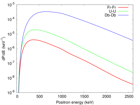
Figure 2: (Color online) Positron energy spectrum for the Fr$-$Fr, U$-$U, and Db$-$Db head-on collisions at energies 674.5, 740, and 928.4 MeV, respectively.

In Fig. 3, we present the number of created pairs $P$ in head-on collisions of two identical nuclei as a function of the nuclear charge $Z_{A}=Z_{B}=Z$ for the projectile energy $E_{0}=6.2$ MeV/u in the nuclear rest frame, which corresponds to $E_{\rm cm}=740$ MeV for the U$-$U collisions.

Figure 3: Number of created pairs $P$ in the head-on collision of identical nuclei as a function of the nuclear charge $Z_{A}=Z_{B}=Z$ for the projectile energy $E_{0}=6.2$ MeV/u in the nuclear rest frame.

There is a very strong dependence of $P$ on $Z$, which in the subcritical region $78\leq Z\leq 87$ can be parametrized by $Z^{\gamma}$ with $\gamma\approx 28$. The function $P(Z)$ smoothly continues into the supercritical region $Z>87$, but its growth is slowing down for the higher $Z$. This result is very close to the corresponding one in Ref. Reinhardt_81 , where it was found that in collisions of bare nuclei, the positron production is proportional to $(Z_{A}+Z_{B})^{\gamma}$ with $\gamma\approx 29$.

In order to demonstrate the ability of our method to describe the spontaneous pair creation we considered the supercritical U$-$U and subcritical Fr$-$Fr collisions with artificial trajectories at $E_{\rm cm}=674.5$ and $E_{\rm cm}=740$ MeV, respectively. First, we introduce the new trajectory $R_{\alpha}(t)$,

$$\dot{R}_{\alpha}(t)=\alpha\dot{R}(t),$$ (31)

where $R(t)$ is the classical Rutherford trajectory. In Fig. 4, we present the number of created pairs $P$ as a function of $\alpha$ for the U$-$U and Fr$-$Fr head-on collisions.

Figure 4: Number of created pairs $P$ in the head-on collision with the artificial trajectory $R_{\alpha}(t)$, defined by Eq. (31), as a function of $\alpha$. The solid line indicates the results for the Fr$-$Fr collision at $E_{\rm cm}=674.5$ MeV; the dashed line corresponds to the U$-$U collision at $E_{\rm cm}=740$ MeV.

It can be seen that in both cases $P(\alpha)$ grows monotonically for large $\alpha$, which can be explained by an enhancement of the dynamical pair production due to the fast variation of the potential. For small values of $\alpha$, where the dynamical mechanism is suppressed, $P(\alpha)$ increases for the U$-$U collision and goes to zero for the Fr$-$Fr collision, which indicates the existence of the spontaneous pair creation in the supercritical case.

We also considered the trajectories with the time delay $T$ at the closest approach of the nuclei. Such trajectories can be used to model the hypothetical collisions with the nuclear sticking Greiner_85 . In the supercritical case the time delay should enhance the spontaneous pair creation. The obtained positron spectra for the pure Rutherford trajectory ($T=0$) and for the different time delays in the head-on Fr$-$Fr and U$-$U collisions are shown in Figs. 5 and 6, respectively. As can be seen from Fig. 5, the shape of the positron spectrum is changed significantly with growing $T$. However, the variations of the total number of created pairs $P$ for the Fr$-$Fr collisions are less than 15% and are oscillating. In the supercritical U$-$U collisions, $P$ increases monotonically as $T$ grows, which demonstrates the enhancement of the spontaneous pair creation. It can be seen from the figures that some additional peaks appear for large $T$ in both cases. However, in the supercritical case, the main peak is much higher than the others and steadily grows and shifts towards the low energies with increasing $T$. This leads to the conclusion that the spontaneous mechanism predominantly contributes to the region of the main peak for the largest $T$. Our results for the positron spectra in the U$-$U collisions with the time delay are in good agreement with the corresponding ones from Ref. Muller_88 , and differ from the values obtained in Ref. Ackad_08 , especially for the small positron energies.

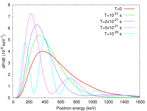
Figure 5: (Color online) Positron energy spectrum for the Fr$-$Fr head-on collision at $E_{\rm cm}=674.5$ MeV with different time delays $T$.

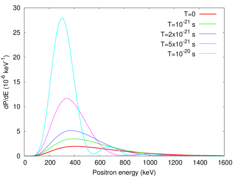
Figure 6: (Color online) Positron energy spectrum for the U$-$U head-on collision at $E_{\rm cm}=740$ MeV with different time delays $T$.

IV CONCLUSION

We presented a method for calculations of pair production in low-energy collisions of bare nuclei. Using this method, the energy spectra of emitted positrons and the numbers of created pairs in collisions of identical nuclei were calculated in the monopole approximation for different values of the impact parameter and the nuclear charge. The ability of the method to describe the spontaneous pair creation was demonstrated by calculations for the collisions with the modified velocity and with the time delays.

The obtained results for the U$-$U collisions are in good agreement with the corresponding values from Ref. Muller_88 for all considered impact parameters. The calculations showed a very strong dependence of the dynamical pair creation on the nuclear charge, which confirms the results of Ref. Reinhardt_81 . The calculated positron energy spectra for the U$-$U, Fr$-$Fr, and Db$-$Db head-on collisions disagree with those presented in Ref. Ackad_08 . The reason for this discrepancy is unclear to us.

A comparison of the different subcritical and supercritical scenarios leads to the conclusion that no direct evidence of the spontaneous pair creation can be found in the positron energy spectra for the heavy-ion collisions with the Rutherford trajectory. We expect, however, that the detailed studies of various processes that take place in low-energy heavy-ion collisions, including the angular-resolved positron energy spectra, can examine the validity of QED at the supercritical regime. For these studies, more elaborated full three-dimensional methods are needed. To date, such methods have been developed for calculations of the electron-excitation and charge-transfer probabilities only Tup_10 ; Tup_12 ; Kozhedub_2013 ; Maltsev_2013 ; Deyneka_13 ; Kozhedub_14 . The extension of these methods to calculations of pair-production probabilities is one of the main goals of our future work.

References

- (1) I. Pomeranchuk and J. Smorodinsky, J. Phys. USSR 9, 97 (1945).
- (2) S. S. Gershtein and Y. B. Zeldovich, Zh. Eksp. Teor. Fiz. 57, 654 (1969) [Sov. Phys. JETP 30, 358 (1970)].
- (3) W. Pieper and W. Greiner, Z. Phys. 218, 327 (1969).
- (4) Y. B. Zeldovich and V. S. Popov, Sov. Phys. Usp. 14, 673 (1972).
- (5) W. Greiner, B. Müller, and J. Rafelski, Quantum Electrodynamics of Strong Fields, (Springer-Verlag, Berlin, 1985).
- (6) U. Müller-Nehler and G. Soff, Phys. Rep. 246, 101 (1994).
- (7) Conceptual Design Report: An International Accelerator Facility for Beams of Ions and Antiprotons, edited by W. Henning (GSI, Darmstadt, 2001).
- (8) A. Gumberidze et al., Nucl. Instrum. Methods Phys. Res., Sect. B 267, 248 (2009).
- (9) S. S. Gershtein and V. S. Popov, Lett. Nuovo Cimento 6, 593 (1973).
- (10) V. S. Popov, Zh. Eksp. Teor. Fiz. 65, 35 (1973) [Sov. Phys. JETP 38, 18 (1974)].
- (11) H. Peitz, B. Müller, J. Rafelski, and W. Greiner, Lett. Nuovo Cimento 8, 37 (1973).
- (12) J. Reinhardt, B. Müller, and W. Greiner, Phys. Rev. A 24, 103 (1981).
- (13) U. Müller, T. de Reus, J. Reinhardt, B. Müller, W. Greiner, and G. Soff, Phys. Rev. A 37, 1449 (1988).
- (14) P. Küprick, H. J. Lüdde, W.-D. Sepp, and B. Fricke, Z. Phys. D 25, 17 (1992).
- (15) E. Ackad and M. Horbatsch, J. Phys.: Conf. Ser. 88, 012017 (2007).
- (16) E. Ackad and M. Horbatsch, Phys. Rev. A 78, 062711 (2008).
- (17) I. I. Tupitsyn, Y. S. Kozhedub, V. M. Shabaev, G. B. Deyneka, S. Hagmann, C. Kozhuharov, G. Plunien, and Th. Stöhlker, Phys. Rev. A 82, 042701 (2010).
- (18) I. I. Tupitsyn, Y. S. Kozhedub, V. M. Shabaev, A. I. Bondarev, G. B. Deyneka, I. A. Maltsev, S. Hagmann, G. Plunien, and Th. Stöhlker, Phys. Rev. A 85, 032712 (2012).
- (19) Y. S. Kozhedub, I. I. Tupitsyn, V. M. Shabaev, S. Hagmann, G. Plunien, and Th. Stöhlker, Phys. Scr. T156, 014053 (2013).
- (20) I. A. Maltsev, G. B. Deyneka, I. I. Tupitsyn, V. M. Shabaev, Y. S. Kozhedub, G. Plunien, and Th. Stöhlker, Phys. Scr. T156, 014056 (2013).
- (21) G. B. Deyneka, I. A. Maltsev, I. I. Tupitsyn, V. M. Shabaev, A. I. Bondarev, Y. S. Kozhedub, G. Plunien, and Th. Stöhlker, Eur. Phys. J. D 67, 258 (2013).
- (22) Y. S. Kozhedub, V. M. Shabaev, I. I. Tupitsyn, A. Gumberidze, S. Hagmann, G. Plunien, and Th. Stöhlker, Phys. Rev. A 90, 042709 (2014).
- (23) A. I. Bondarev, Y. S. Kozhedub, I. I. Tupitsyn, V. M. Shabaev, and G. Plunien, Phys. Scr. T156, 014054 (2013).
- (24) S. R. McConnell, A. N. Artemyev, M. Mai, and A. Surzhykov, Phys. Rev. A 86, 052705 (2012).
- (25) I. B. Khriplovich, JETP Lett. 100, 494 (2014).
- (26) V. M. Shabaev, I. I. Tupitsyn, V. A. Yerokhin, G. Plunien, and G. Soff, Phys. Rev. Lett. 93, 130405 (2004).
- (27) V. M. Shabaev, K. Pachucki, I. I. Tupitsyn, and V. A. Yerokhin, Phys. Rev. Lett. 94, 213002 (2005).
- (28) Y. S. Kozhedub, A. V. Volotka, A. N. Artemyev, D. A. Glazov, G. Plunien, V. M. Shabaev, I. I. Tupitsyn, and Th. Stöhlker, Phys. Rev. A 81, 042513 (2010).
- (29) E. S. Fradkin, D. M. Gitman, and S. M. Shvartsman, Quantum Electrodynamics with Unstable Vacuum, (Springer-Verlag, Berlin, 1991).
- (30) P. W. Langhoff, J. Sims, and C. T. Corcoran, Phys. Rev. A 10, 829 (1974).
- (31) J. Crank and P. Nicolson, Proc. Cambridge Philos. Soc. 43, 50 (1947).
- (32) P. Joly and G. Meurant, Numerical Algorithms 4, 379 (1993).
- (33) C. de Boor, A Practical Guide to Splines, Applied Mathematical Sciences, Vol. 27, revised edition (Springer-Verlag, New York, 2001).
- (34) W. R. Johnson, S. A. Blundell, and J. Sapirstein, Phys. Rev. A 37, 307 (1988).