A Stochastic Model of Inward Diffusion in Magnetospheric Plasmas

Abstract

The inward diffusion of particles, often observed in magnetospheric plasmas (either naturally created stellar ones or laboratory devices) creates a spontaneous density gradient, which seemingly contradicts the entropy principle. We construct a theoretical model of diffusion that can explain the inward diffusion in a dipole magnetic field. The key is the identification of the proper coordinates on which an appropriate diffusion operator can be formulated. The effective phase space is foliated by the adiabatic invariants; on the symplectic leaf, the invariant measure (by which the entropy must be calculated) is distorted, by the inhomogeneous magnetic field, with respect to the conventional Lebesgue measure of the natural phase space. The collision operator is formulated to be consistent to the ergodic hypothesis on the symplectic leaf, i.e., the resultant diffusion must diminish gradients on the proper coordinates. The non-orthogonality of the cotangent vectors of the configuration space causes a coupling between the perpendicular and parallel diffusions, which is derived by applying Ito’s formula of changing variables. The model has been examined by numerical simulations. We observe the creation of a peaked density profile that mimics radiation belts in planetary magnetospheres as well as laboratory experiments.

I Introduction

Spontaneous creation of plasma clump is commonly observed in the vicinity of various-scale dipole magnetic fields, ranging from planetary magnetospheres Voy1 ; Voy2 ; CRPWSE to laboratory plasma devices Yos4 ; Box . However, if one were biased by the textbook knowledge that plasma particles are “diamagnetic”, it is somewhat mysterious how a magnetic dipole can attract charged particles. Or, if one calculates the Boltzmann distribution of charged particles, one finds that the density does not respond to magnetic field. We have to develop a reasonable model to explain how the inward diffusion (or, up-hill diffusion) can take place to create a density gradient in a dipole magnetic field —this is a theoretical challenge because the creation of gradient is seemingly contradicting the entropy principle.

The early works on the topic, mainly theoretical, date back to the $1960$s Falt ; Bir . The concept of electromagnetic fluctuations driven radial diffusion was investigated, and a coarse-grained kinetic equation in magnetic coordinates was derived by a perturbation method. The key idea is the use of the scale separation, i.e., the time scale over which the first and second adiabatic invariants (magnetic moment and bounce action respectively) are conserved is much longer than the characteristic time scale destroying the third adiabatic invariant (magnetic flux).

On the other hand, some more empirical models of radial diffusion were developed to explain actual observations in the Earth’s magnetosphere: in Spj ; Corn the radial diffusion parameter is evaluated by assuming an $\nu^{-2}$ spectrum, with $\nu$ the frequency of the electromagnetic fluctuations. The main conclusion was that radial diffusion plays a central role in determining the stationary density profile. This diffusion parameter was used in more recent works Fok2 ; Zheng that deal with a bounce-averaged kinetic equation (see also Fok1 ; Fok3 ) describing the electron radiation belts environment of our planet.

Stimulated by the Voyager $1$ and $2$ missions to Saturn Voy1 ; Voy2 and, more recently, by the Cassini Radio and Plasma Wave Science experiment CRPWSE , intensive studies were made to explain the parallel pressure profile along magnetic surfaces ($L$-shells) by the stationary force balance Per1 ; Per2 ; Per3 ; Rich1 ; Rich2 . As explained in Rich1 , the underlying assumption is that transport in the inner magnetosphere is driven by radial diffusion.

A common understanding is that the particle number per flux-tube volume tends to be homogenized (see for example Has ; Schippers ), hence, a diffusion equation should be written on a magnetic coordinate system. Transforming back to the ordinary Cartesian coordinates, we observe the inward diffusion, because a thinner flux tube near the magnetic dipole will have a higher density.

Recently, the idea of using the magnetic coordinates was put into the perspective of phase-space foliation (or, degenerate Poisson algebra), by which a “macro-scale hierarchy” was given a mathematical formulation as a leaf of Casimir invariants YosFol . An adiabatic invariant translates into a Casimir invariant of noncanonical Hamiltonian system that describes the dynamics of quasi-particles, i.e., the representations of coarse-grained particles ignoring the microscopic action-angle degree of freedom. The scale of adiabaticity separates macro and micro hierarchies (reversing the viewpoint, we can interpret a Casimir invariant as some adiabatic invariant, and formulate a singular perturbation unfreezing the corresponding topological constraint YosFol2 ; YosFol3 ). By maximizing the entropy on a symplectic leaf (Poisson submanifold) of the phase space, we can derive a Boltzmann distribution of quasi-particles. Embedding the leaf into the total phase space on the laboratory frame, we obtain a clump of magnetized particles that simulates experimental observations (see Yos4 ; Yos ; Saitoh ).

The aim of this work is to develop a diffusion model on the foliated phase space. The stochasticity stems in the macro hierarchy; we consider a turbulence of collective modes producing a random perturbation $-\nabla\delta\phi$ of macroscopic electric field, which drives $\boldsymbol{E}\times\boldsymbol{B}$ drifts of the magnetized particles (we assume that particle collisions can be neglected, so that the magnetic moment $\mu$ is an adiabatic invariant). Due to the inhomogeneity of the magnetic field $\boldsymbol{B}=\nabla\psi\times\nabla\theta$ ($\psi$ is the magnetic flux function, and $\theta$ is the toroidal angle), this mechanism gives rise to an inhomogeneous random walk.

There are some delicate problems that need to be carefully addressed in formulating the Fokker-Planck equation. They are primarily due to the $\boldsymbol{E}\times\boldsymbol{B}$ drift approximation and the complexity (non-orthogonality) of the canonical coordinate system. While the proper coordinate system (bearing an invariant measure) is identified as a symplectic leaf of the Casimir (adiabatic) invariant, the macroscopic Hamiltonian needs a subtle amendment in order to describe the $\boldsymbol{E}\times\boldsymbol{B}$ drift (see Cary as well as footnote 1 of YosFol ). Neglecting the kinetic part $mrv_{\theta}$ of the canonical toroidal momentum $P_{\theta}=mrv_{\theta}+q\psi$ ($m$ is the mass, $q$ is the charge, and $r$ is the radius), we approximate $P_{\theta}\approx q\psi$, and then, a canonical equation $\dot{\psi}=\partial_{\theta}\delta\phi$ describes the $\boldsymbol{E}\times\boldsymbol{B}$. Here, we have used the action variable $\psi$ as a spatial coordinate (in fact, the $\boldsymbol{E}\times\boldsymbol{B}$ drift velocity, not the acceleration, is proportional to the electric force). To span the configuration space, we introduce a parallel coordinate $\ell$ along each field line (contour of $\psi$). The cotangent vectors $d\psi$ and $d\ell$ are not orthogonal; hence, we need an appropriate “drift energy” in the Hamiltonian to produce $\dot{\ell}$ associated with the perpendicular drift velocity. Instead of following the rather complicated Hamiltonian formalism to determine the diffusion operator, we may reverse the process of formulation. We start by assuming a random $\boldsymbol{E}\times\boldsymbol{B}$ drift velocity $\dot{\boldsymbol{X}}$ in the natural coordinates (i.e.,the velocity is a member of the tangent bundle); we consider a Wiener process, in the perpendicular direction, multiplied by an unknown amplitude. We transform it to the canonical variables by invoking Ito’s formula of coordinate transformations. The diffusion coefficient must be made constant on the canonical coordinate system, by which the amplitude of the Wiener process is determined. The derived diffusion equation has an interesting “drift terms” describing the geometrical coupling of the two spatial coordinates $\psi$ and $\ell$.

II Invariant Measure

We start by reviewing the phase-space foliation due to the constraint of adiabatic invariant (here, the magnetic moment). We consider a macroscopic system of magnetized particles; the macro-scale hierarchy is formally defined by separating the microscopic action-angle variables $\mu$-$\theta_{c}$ ($\mu=mv_{c}^{2}/(2B)$ is the magnetic moment, $v_{c}$ is the cyclotron velocity, and $\theta_{c}$ is the gyration angle) from the total action of charged particles. Then, the actual phase space is a sub-manifold (leaf) of the 6-dimensional phase space ($\mu$-space), which is a symplectic leaf span by the canonical variables $(\ell,v_{\parallel},\psi,\theta)$, where $\ell$ is the arch-length along magnetic field lines defined by $\partial_{\ell}=\boldsymbol{B}/B$, $v_{\parallel}$ is the velocity parallel to field lines, $\psi$ is the toroidal angular momentum (neglecting the mechanical part $mrv_{\theta}$) and $\theta$ is the toroidal angle. Regarding $\mu$ as an attribute of each particle, we consider statistical mechanics on this symplectic leaf. The natural invariant measure is, after separating the microscopic variables,

$$dV_{m}=d\ell dv_{\parallel}d\psi d\theta.$$ (1)

We consider the Wiener process that tends to maximize the entropy counted by this measure.

Let us see the relation between the laboratory frame and the symplectic leaf of magnetized particles. The volume element of the former is, in the $(r,z,\theta)$ cylindrical coordinates,

$$dV=rdrdzd\theta dv_{\parallel}dv_{\perp}dv_{\theta},$$ (2)

where $v_{\perp}$ is the perpendicular velocity, and $v_{\theta}$ is the toroidal velocity. Neglecting the toroidal drift velocity with respect to the cyclotron velocity $v_{c}$, we may approximate $v_{\perp}=v_{c}$, and then,

$$dV=rdrdzd\theta dv_{\parallel}v_{c}dv_{c}d\theta_{c}=\frac{B}{m}rdrdzd\theta dv_{\parallel}d\mu d\theta_{c}.$$ (3)

Using $|\nabla\ell\cdot\nabla\psi\times\nabla\theta|=B$, we may write

$$dV=\frac{1}{m}d\ell d\psi d\theta dv_{\parallel}d\mu d\theta_{c}.$$ (4)

On the symplectic leaf, $\psi$ and $\ell$ play the role of spatial coordinates (the functional forms of $\psi(r,z)$ and $\ell(r,z)$ are given in appendix A). The spacial volume of the laboratory frame and that of the symplectic leaf are related by

$$d^{3}x=\frac{dV}{dv_{\parallel}dv_{\perp}dv_{\theta}}=\frac{m}{B}\frac{dV}{dv_{\parallel}d\mu d\theta_{c}}=\frac{2\pi}{B}d\ell d\psi.$$ (5)

The Jacobian weight $B/2\pi$ is the noted factor that multiplies to the symplectic-leaf density.

III Stochastic Motion of Particles

III.1 Perpendicular Motion by $\boldsymbol{E}\times\boldsymbol{B}$ Drift

Here consider electrostatic fluctuations as the causal of transport on the symplectic leaf of magnetized particles. Upon the $\boldsymbol{E}\times\boldsymbol{B}$ drift approximation (we neglect the higher-order polarization drift), the velocity in the direction normal to flux surfaces is given by

$$\boldsymbol{v}_{\perp}=\frac{\delta\boldsymbol{E}\times\boldsymbol{B}}{B^{2}}=\frac{\delta E_{\theta}}{B}\partial_{\perp}=-\frac{1}{rB}\frac{\partial\delta\phi}{\partial\theta}\partial_{\perp}.$$ (6)

Here $\partial_{\perp}$ stands for the unit vector in the normal direction:

$$\partial_{\perp}=\frac{\nabla\psi}{|\nabla\psi|}=\frac{\nabla\psi}{rB}.$$ (7)

We assume

$$\langle\delta\phi(t)\rangle=0,$$ (8a)

$$\langle\delta\phi(t)\delta\phi(s)\rangle\propto\delta(t-s).$$ (8b)

The standard assumptions (8b) and (8b), respectively, mean the average charge neutrality and the de-correlation of the fluctuation at the scale of the present macroscopic model, i.e., $\delta\phi$ is a Gaussian white noise. The drift velocity $v_{\perp}$ of equation (6) is given by

$$dX_{\perp}=v_{\perp}dt=\frac{D_{\perp}^{1/2}}{rB}dW_{\perp},$$ (9)

where $dW_{\perp}=\Gamma_{\perp}(t)dt$ is a Wiener process Elia acting in the direction perpendicular to the flux surfaces, and $D_{\perp}^{1/2}(\boldsymbol{z})$, with $\boldsymbol{z}=(\ell,\psi,v_{\parallel},\mu)$, is the magnitude of fluctuations, which will be determined in sec. V. We denote random variables by upper-case letters.

III.2 Parallel Motion

The equation of motion in the parallel direction is written as

$$m\frac{dv_{\parallel}}{dt}=-\mu\frac{\partial B}{\partial\ell}-q\frac{\partial\delta\phi}{\partial\ell}-m\gamma v_{\parallel}.$$ (10)

The first term on the right hand side is the mirror force. The third term is a friction force ($\gamma$ is the friction coefficient). The parallel electric field is usually much smaller than the perpendicular one. We assume

$$-\frac{q}{m}\frac{\partial\delta\phi}{\partial\ell}=D_{\parallel}^{1/2}\frac{dW_{\parallel}}{dt},$$ (11)

The amplitude $D_{\parallel}^{1/2}$ is a constant since $v_{\parallel}$ is a canonical variable on which the diffusion coefficient has to be Fickian.

The stochastic equation of motion in the parallel direction reads

$$dV_{\parallel}=-\left(\frac{\mu}{m}\frac{\partial B}{\partial\ell}+\gamma v_{\parallel}\right)dt+D_{\parallel}^{1/2}dW_{\parallel}.$$ (12)

The stochastic evolution of the coordinate $\ell$ (which will be denoted by $L$) is not simply the time integral of $v_{\parallel}$, because particles are moving on the curvilinear coordinates: due to $\nabla\ell\cdot\partial_{\perp}\not=0$ a velocity in $\partial_{\perp}$ also causes a change in $\ell$. Including this effect, we obtain (see appendix D for the derivation)

$$dL=\left\{v_{\parallel}+\left(\frac{1}{2}-\alpha\right)D_{\perp}\left[\left(\mathfrak{q}\frac{\partial}{\partial\ell}+\frac{\partial}{\partial\psi}\right)\mathfrak{q}+\mathfrak{q}\left(\mathfrak{q}\frac{\partial}{\partial\ell}+\frac{\partial}{\partial\psi}\right)\ln(rB)\right]\right\}dt+\mathfrak{q}D_{\perp}^{1/2}dW_{\perp},$$ (13)

where the geometrical factor $\mathfrak{q}$ is defined by

$$\mathfrak{q}=\frac{\nabla\ell\cdot\nabla\psi}{(rB)^{2}}.$$ (14)

The coefficient $\alpha$ will be explained in the next section.

IV Stochastic Integrals

In the previous section, we have derived a system of stochastic differential equations (SDEs) (9), (12), and (13). To obtain the corresponding Fokker-Planck equation (FPE) we need a rigorous definition of the stochastic integral that determines the solution to our equations of motion. Indeed, While the deterministic terms (multiplied by $dt$) can be integrated by the usual Riemann integral, the random terms (multiplied by $dW$) require careful treatment. One may integrate a stochastic term differently depending on the choice of $t_{\alpha}\in[t_{i-1},t_{i}]$ ($t_{i-1}$ and $t_{i}$ are neighbouring times) Gar ; Ris ; Evans . Let us do a practice with the perpendicular equation (9). If we put $t_{\alpha}=t_{i-1}+\alpha\Delta t_{i}$ with $\alpha\in[0,1]$, approximate the integral with a finite sum, and then take the limit for $\Delta t_{i}=\frac{t-t_{0}}{n}\rightarrow 0$ as in the Riemann integral, we have

$$\begin{split}\int_{t_{0}}^{t}dX_{\perp}=ms\text{-}\lim_{n\to\infty}\sum_{i=1}^{n}&\frac{D_{\perp}^{1/2}}{rB}\left(\boldsymbol{X}(t_{\alpha})\right)\\ &[W_{\perp}(t_{i})-W_{\perp}(t_{i-1})].\end{split}$$ (15)

Here ”$ms$” stands for mean-square limit and $\boldsymbol{X}(s)$ denotes the position in space at time $s$. Note that $\boldsymbol{X}$ is a random process. Because of the nowhere differentiability Evans of the Wiener process, the value of the integral (15) depends on $\alpha$. This problem is known as the Ito-Stratonovich dilemma (the reader is referred to Wong ; Kampen ; Kampen2 ; Kuroiwa ; Moon ; Sancho ; Chechkin ; Ran ; Yuan ; Farago ; Volpe ; Mannella ; Lau ). In appendix C, we give a theorem which establishes the relationship between the Ito integral $\alpha=0$ Gar ; Ris ; Evans ; Ito1 ; Ito3 ; Ito4 and that calculated with a different $\alpha$. As an alternative to Ito’s definition, the Stratonovich integral assumes $\alpha=1/2$ Gar ; Ris ; Evans .

In the case of homogeneous random walks, all the definitions of the stochastic integral are equivalent (see appendix C). However, in an inhomogeneous random walk, FPE depends on $\alpha$.

We have to choose an appropriate $\alpha$ by examining the physical information contained in $\alpha$. The Ito integral with $\alpha=0$ assumes that two neighboring values of the Wiener process are connected by a step function. More precisely, if we combine a Poisson process $\mathcal{P}_{\lambda}$, which samples the times at which fluctuations occur (with rate $\lambda$), and a Gaussian process $N(0,t)$, which samples the amplitude of the fluctuations, we have a process that converges to the Wiener process $W$ equipped with Ito’s definition of the stochastic integral in the limit $\lambda\rightarrow\infty$. In fact, the integral of a function $f$ over the process $\mathcal{P}_{\lambda}\otimes N$ is (see figure 1a)

$$I=ms\text{-}\lim_{n\rightarrow\infty}\sum_{i=1}^{n}f(t_{i-1})(W(t_{i})-W(t_{i-1})),$$ (16)

and the probability distribution $P_{\lambda}(x,t)$ of having an amplitude $x$ of the fluctuations at time $t$ converges to a normal distribution $N(0,t)$ with variance $t$:

$$P_{\lambda}(x,t)=\frac{1}{\sqrt{2\pi t}}e^{-x^{2}/2t}(1-e^{-\lambda t})+\delta(x)e^{-\lambda t}\xrightarrow{\lambda\rightarrow\infty}\frac{1}{\sqrt{(2\pi t)}}e^{-x^{2}/2t}.$$ (17)

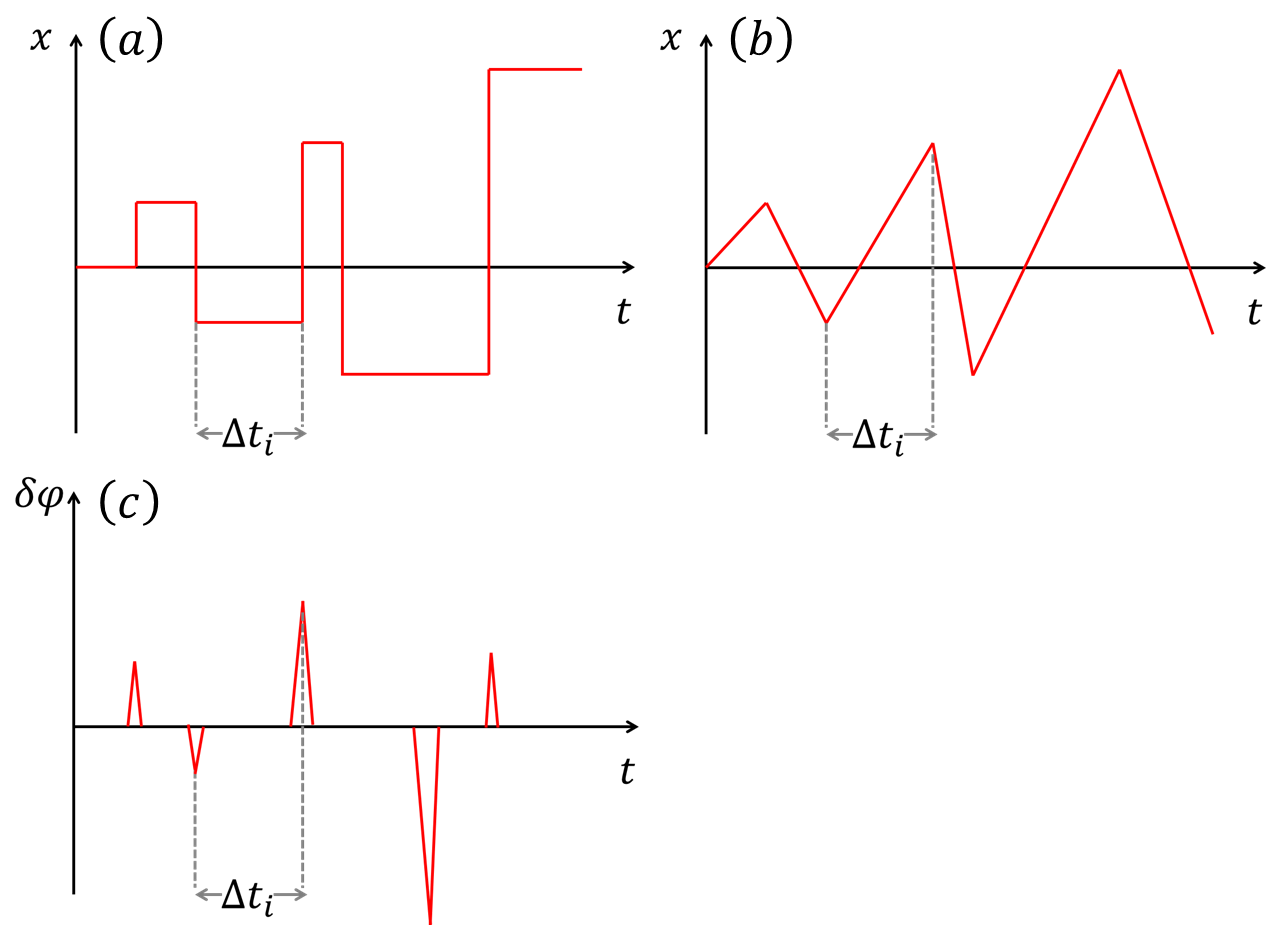
Figure 1: (a): schematic representation of the process $\mathcal{P}_{\lambda}\otimes N$. In the limit $\lambda\rightarrow\infty$ it converges to the Wiener process equipped with Ito’s integral. (b): schematic representation of the process $\mathcal{P}_{\lambda}\otimes N^{\prime}$. In the limit $\lambda\rightarrow\infty$ it converges to the Wiener process equipped with Stratonovich integral $\alpha=1/2$. (c): schematic representation of the turbulent electric potential $\delta\phi$.

Consider now a new process $\mathcal{P}_{\lambda}\otimes N^{\prime}$ where this time $N^{\prime}(0,t)$ is a normal distribution that samples the angular coefficient. The integral of a function $f$ over this new process is

$$I^{\prime}=ms\text{-}\lim_{n\rightarrow\infty}\sum_{i=1}^{n}f\left(t_{i-1}+\frac{\Delta t_{i}}{2}\right)(W(t_{i})-W(t_{i-1})),$$ (18)

and the probability distribution $P^{\prime}_{\lambda}(x,t)$ of having an amplitude $x$ of the fluctuations at time $t$ converges to a normal distribution $N(0,t)$ with variance $t$ (the proof is given by representing the process as $x(t)=x_{i-1}+\frac{t-t_{i-1}}{t_{i}-t_{i-1}}(x_{i}-x_{i-1})$ and verifying that its variance goes to $t$ in the limit $\lambda\rightarrow\infty$). A schematic representation of this new process is given in figure 1b.

In bounce motion, a particle experiences random kicks by the turbulent potential $\delta\phi$ (see figure 1c), which are the temporal derivatives of Ito’s $W$ shown in figure 1a. Indeed, $\delta\phi\propto\Gamma(t)=dW/dt$ (see (8a) and (8b)). Hence, we choose $\alpha=0$, i.e., Ito’s definition of the stochastic integral.

V Coordinate Transformation to the Proper Frame

For a diffusion process to homogenize the probability distribution with respect to the invariant measure, the diffusion coefficient (the magnitude of the white noise) must be constant on the symplectic leaf (proper frame); in (9), we have to change the coordinate $X_{\perp}$ to $\Psi$:

$$d\Psi=Adt+D_{\psi}^{1/2}dW_{\perp},$$ (19)

with $D_{\psi}^{1/2}$ a constant diffusion coefficient and $A$ a drift current.

To evaluate $A$ we apply Ito’s lemma of changing variables (from $X_{\perp}$ to $\Psi$) of stochastic calculus Gar ; Ris ; Evans (since the rule for an arbitrary $\alpha$ is not found in the literature, we derive it in appendix B). By equations (9), (19), and (46), we obtain

$$A=\left(\frac{1}{2}-\alpha\right)\frac{D_{\perp}}{(rB)^{2}}\frac{\partial^{2}\psi}{\partial x_{\perp}^{2}},$$ (20a)

$$D_{\psi}^{1/2}=\frac{D_{\perp}^{1/2}}{rB}\left(\frac{\partial\psi}{\partial x_{\perp}}\right).$$ (20b)

By

$$\frac{\partial\psi}{\partial x_{\perp}}=\nabla\psi\cdot\partial_{\perp}=\frac{\nabla\psi\cdot\nabla\psi}{rB}=rB,$$ (21)

we obtain $D_{\perp}^{1/2}=D_{\psi}^{1/2}$ = constant, and

$$A=\left(\frac{1}{2}-\alpha\right)\frac{D_{\perp}}{(rB)^{2}}\frac{\partial}{\partial x_{\perp}}rB=\left(\frac{1}{2}-\alpha\right)\frac{D_{\perp}}{(rB)^{2}}\left(\frac{\partial\ell}{\partial x_{\perp}}\frac{\partial}{\partial\ell}+\frac{\partial\psi}{\partial x_{\perp}}\frac{\partial}{\partial\psi}\right)rB=\left(\frac{1}{2}-\alpha\right)\frac{D_{\perp}}{(rB)^{2}}\left(\frac{\partial\ell}{\partial x_{\perp}}\frac{\partial}{\partial\ell}+rB\frac{\partial}{\partial\psi}\right)rB.$$ (22)

We have

$$\frac{\partial\ell}{\partial x_{\perp}}=\nabla\ell\cdot\partial_{\perp}=\frac{\nabla\ell\cdot\nabla\psi}{rB}.$$ (23)

Combining (22) and (23), we obtain

$$A=D_{\perp}\left(\frac{1}{2}-\alpha\right)\left(\frac{\nabla\ell\cdot\nabla\psi}{(rB)^{2}}\frac{\partial}{\partial\ell}+\frac{\partial}{\partial\psi}\right)\ln\left(rB\right).$$ (24)

In summary,

$$d\Psi=D_{\perp}\left(\frac{1}{2}-\alpha\right)\left(\mathfrak{q}\frac{\partial}{\partial\ell}+\frac{\partial}{\partial\psi}\right)\ln\left(rB\right)dt\\ +D_{\perp}^{1/2}dW_{\perp}.$$ (25)

VI Fokker-Planck Equation

Given a system of SDEs such as

$$dX_{i}=F_{i}dt+G_{ij}dW_{j},$$ (26)

and the stochastic integral is defined with an appropriate $\alpha$ (we assume that $\alpha$ is common for all Wiener processes $W_{j}$), the Fokker-Planck equation governing the probability density $f$ is Gar ; Ris

$$\frac{\partial f}{\partial t}=\frac{\partial}{\partial x_{i}}\left(-F_{i}+\frac{1}{2}\frac{\partial}{\partial x_{j}}G_{ik}G_{jk}-\alpha\frac{\partial G_{ik}}{\partial x_{j}}G_{jk}\right)f.$$ (27)

Using (12), (13) and (25) in (27), we obtain

$$\frac{\partial P}{\partial t}=-v_{\parallel}\frac{\partial P}{\partial\ell}+\frac{\partial}{\partial v_{\parallel}}\left[\left(\frac{\langle\mu\rangle_{\boldsymbol{v}}}{m}\frac{\partial B}{\partial\ell}+\gamma v_{\parallel}\right)P\right]-\left(\frac{1}{2}-\alpha\right)D_{\perp}\frac{\partial}{\partial\psi}\left\{\left[\left(\mathfrak{q}\frac{\partial}{\partial\ell}+\frac{\partial}{\partial\psi}\right)\ln{(rB)}\right]P\right\}-\left(\frac{1}{2}-\alpha\right)D_{\perp}\frac{\partial}{\partial\ell}\left\{\left[\mathfrak{q}\left(\mathfrak{q}\frac{\partial}{\partial\ell}+\frac{\partial}{\partial\psi}\right)\ln{(rB)}\right]P\right\}-\frac{1}{2}D_{\perp}\frac{\partial}{\partial\ell}\left\{\left[\left(\mathfrak{q}\frac{\partial}{\partial\ell}+\frac{\partial}{\partial\psi}\right)\mathfrak{q}\right]P\right\}+\frac{1}{2}D_{\perp}\frac{\partial^{2}}{\partial\ell^{2}}\left(\mathfrak{q}^{2}P\right)+D_{\perp}\frac{\partial^{2}}{\partial\ell\partial\psi}\left(\mathfrak{q}P\right)+\frac{1}{2}D_{\perp}\frac{\partial^{2}P}{\partial\psi^{2}}+\frac{1}{2}D_{\parallel}\frac{\partial^{2}P}{\partial v_{\parallel}^{2}}.$$ (28)

Here $P$ is the probability distribution on the proper frame $(\ell,\psi,v_{\parallel})$, and $\langle\mu\rangle_{\boldsymbol{v}}$ is the average of $\mu$ over the velocity space. The laboratory-frame spatial density $\rho$ is given by

$$\rho=\frac{d\ell d\psi d\theta}{rdrdzd\theta}\int{Pdv_{\parallel}}=|\nabla\ell\cdot\nabla\psi\times\nabla\theta|u=Bu,$$ (29)

where $u=\int{Pdv_{\parallel}}$ is the spatial density on the proper frame. It is now evident in (28) that the diffusion on the coordinate $\psi$ is Fickian with a constant diffusion coefficient, transporting particles to diminish the gradient with respect to $\psi$.

VII Numerical Simulation

We put the formulated model to the test by numerical simulation. For the purpose of proving the principle, we consider a simple geometry generated by a point dipole magnetic field.

VII.1 Model

To simplify the calculations we make the following approximation:

$$dL\simeq v_{\parallel}dt+\mathfrak{q}D_{\perp}^{1/2}dW_{\perp},$$ (30)

i.e., the transport current appearing in (13) is considered to be much smaller than the convective drift $v_{\parallel}$. Then, FPE becomes

$$\frac{\partial P}{\partial t}=-v_{\parallel}\frac{\partial P}{\partial\ell}+\frac{\partial}{\partial v_{\parallel}}\left[\left(\frac{\langle\mu\rangle_{\boldsymbol{v}}}{m}\frac{\partial B}{\partial\ell}+\gamma v_{\parallel}\right)P\right]-\frac{1}{2}D_{\perp}\frac{\partial}{\partial\psi}\left\{\left[\left(\mathfrak{q}\frac{\partial}{\partial\ell}+\frac{\partial}{\partial\psi}\right)\ln{(rB)}\right]P\right\}+\frac{1}{2}D_{\perp}\frac{\partial^{2}}{\partial\ell^{2}}\left(\mathfrak{q}^{2}P\right)+D_{\perp}\frac{\partial^{2}}{\partial\ell\partial\psi}\left(\mathfrak{q}P\right)+\frac{1}{2}D_{\perp}\frac{\partial^{2}P}{\partial\psi^{2}}+\frac{1}{2}D_{\parallel}\frac{\partial^{2}P}{\partial v_{\parallel}^{2}},$$ (31)

where we put $\alpha=0$ as concluded in section IV.

To solve (31), we need to specify $\langle\mu\rangle_{\boldsymbol{v}}$. Here we assume a local Boltzmann distribution as derived in Yos . Since $\mu$ is a robust adiabatic invariant, we may consider a grand canonical ensemble determined by the energy and magnetization (total magnetic moment). Maximizing the entropy, we obtain

$$f^{eq}=\Theta(\ell,\psi,v_{\parallel})e^{-\beta(B+\zeta)\mu},$$ (32)

where $\zeta$ is the Lagrangian multiplier (chemical potential) with respect to the magnetization, $\beta$ the inverse temperature, and $\Theta$ a function independent of $\mu$. Then,

$$\langle\mu\rangle_{\boldsymbol{v}}^{eq}=\frac{\int{\mu f^{eq}d\mu}}{\int{f^{eq}d\mu}}=\frac{1}{\beta(B+\zeta)}.$$ (33)

VII.2 Results of Numerical Simulations

Here we study the free decay of the density starting from an initial Maxwell-Boltzmann distribution in the laboratory frame:

$$P_{lab}(t=0)=BP(t=0)=\sqrt{\frac{m\beta}{2\pi}}\rho_{0}e^{-\beta\frac{m}{2}v_{\parallel}^{2}}.$$ (34)

The corresponding spatial density is, of course, constant ($=\rho_{0}$) in the calculation domain, which is surrounded by a magnetic surface (a level set of $\psi$) as well as a magneto-isobaric surface near the origin $(r,z)=(0,0)$. We assume a homogeneous Dirichlet boundary condition.

We assume that the parallel electric field is much (three orders of magnitude) smaller than the perpendicular electric field. In particular, the characteristic normal and parallel fluctuating potentials are $\delta\phi_{\perp}=500V$ and $\delta\phi_{\parallel}=1V$ acting on typical time scales of $\tau_{\perp}=10\mu s$ and $\tau_{\parallel}=10ns$ so that the non-normalized diffusion parameters are $D_{\perp}=\delta\phi_{\perp}^{2}/\tau_{\perp}=2.5\,10^{10}\,V^{2}s^{-1}$ and $D_{\parallel}=(q\delta\phi_{\parallel})^{2}\tau_{\parallel}/(m\Delta\ell)^{2}=3.1\,10^{24}m^{2}s^{-3}$, where we assumed a typical fluctuation length scale $\Delta\ell=10\mu m$.

Figure 2 shows the change of the total number of particles:

$$N_{tot}=\int_{\partial V}{Pd\ell d\psi dv_{\parallel}}.$$ (35)

Because of the absorbing boundaries, the number of particles contained in the domain decreases.

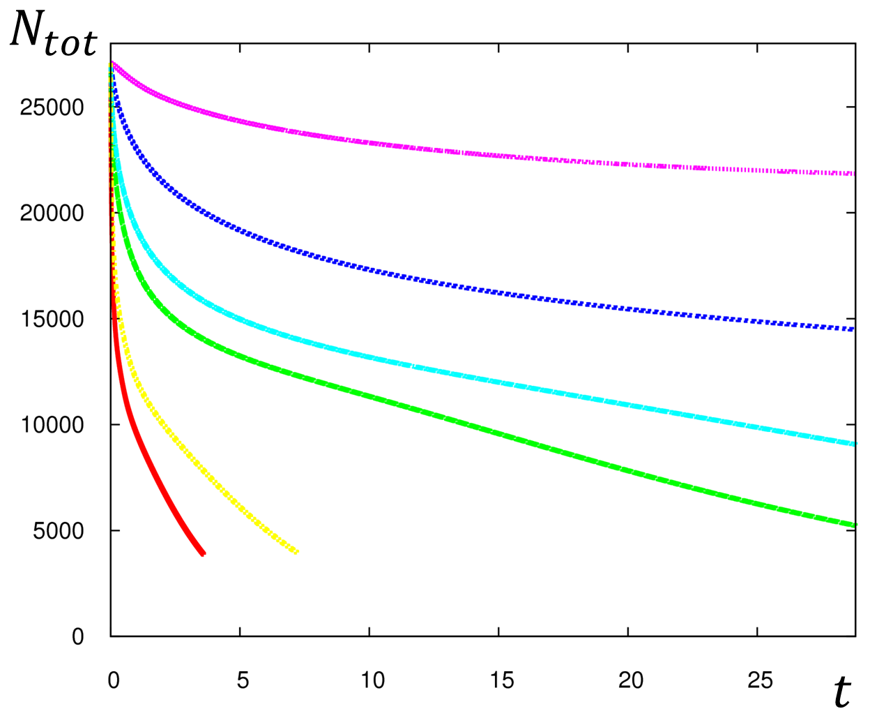
Figure 2: Time evolution of the total particle number $N_{tot}$ in arbitrary units. Time $t$ is calculated as number of numerical steps times the used time step. Different colors correspond to different values of the normal diffusion parameter $D_{\perp}$: purple $10^{-2}D_{\perp}$, blue $10^{-1}D_{\perp}$, sky blue $0.5D_{\perp}$, green $D_{\perp}$, yellow $5D_{\perp}$, and red $10D_{\perp}$.

Figure 3 shows the evolution of the particle density $u$ on the proper frame. Particles are gradually squeezed into the equatorial region; this is due to the mirror effect. At the same time, the profile of $u$ broadens in the direction of $\psi$. Transforming back to the laboratory frame, the corresponding evolution of $\rho$ is viewed as inward diffusion (creation of a density gradient); see figure 4. In the figures, green curves are magnetic field lines (contours of $\psi$), pink curves are the parallel ($\ell$) coordinates, and white curves are the contours of the magnetic field strength.

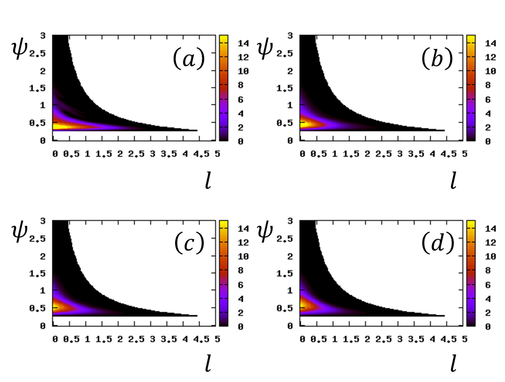
Figure 3: Time evolution of the proper-frame density $u$. (a): $t=0.24$. (b): $t=0.96$. (c): $t=1.68$. (d): $t=2.4$.

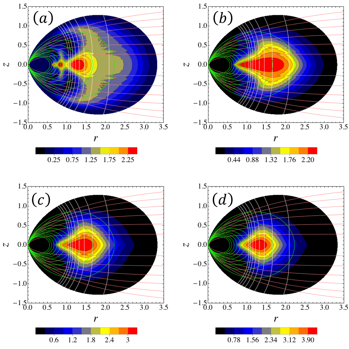
Figure 4: Time evolution of the laboratory frame density $\rho$. (a): $t=0.24$. (b): $t=0.96$. (c): $t=1.68$. (d): $t=2.4$.

Figure 5 shows the evolution of the parallel pressure:

$$\mathcal{P}_{\parallel}=\rho\left\langle\left(v_{\parallel}-\langle v_{\parallel}\rangle\right)^{2}\right\rangle.$$ (36)

The “confinement” in the parallel direction is due the the magnetic mirror effect.

In figure 6, we plot the root mean square parallel velocity:

$$\sqrt{\langle v_{\parallel}^{2}\rangle}=\sqrt{\frac{\int{v_{\parallel}^{2}Pdv_{\parallel}}}{\int{Pdv_{\parallel}}}}=\sqrt{\frac{1}{u}\int{v_{\parallel}^{2}Pdv_{\parallel}}},$$ (37)

which is a measure of the parallel temperature $T_{\parallel}=\frac{m}{2}\langle v_{\parallel}^{2}\rangle$. We observe higher temperatures near the equator.

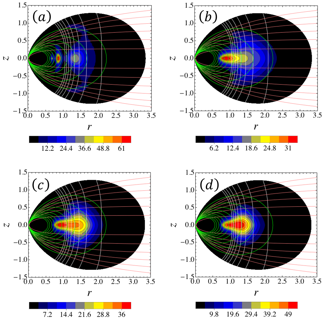
Figure 5: Time evolution of the pressure $\mathcal{P}_{\parallel}$ in the laboratory frame. (a): $t=0.24$. (b): $t=0.96$. (c): $t=1.68$. (d): $t=2.4$.

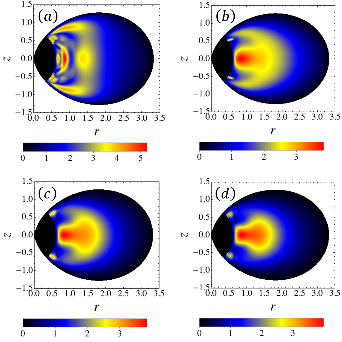
Figure 6: Time evolution of the root mean square velocity $\langle v_{\parallel}^{2}\rangle$ in the laboratory frame. (a): $t=0.24$. (b): $t=0.96$. (c): $t=1.68$. (d): $t=2.4$.

A higher initial temperature $\beta^{-1}$ enables particles to have larger bounce orbits. Consequently, the density may have a wider distribution along field lines. In figure 7, we compare the density distributions (after the same passed) for different initial temperatures.

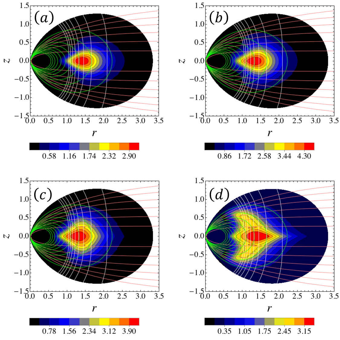
Figure 7: Temperature dependence of the density $\rho$ in the laboratory frame at $t=2.4$. (a): $10^{-2}\beta^{-1}$. (b): $10^{-1}\beta^{-1}$. (c): $\beta^{-1}$. (d): $10\beta^{-1}$

In figure 2, we compare the evolutions with different diffusion coefficients $D_{\perp}$, which, in (31), controls the relative strength of the diffusion effect with respect to the parallel mirror effect. Usually, a stronger diffusion yields a flatter distribution of particles. Here, the opposite is the case in the laboratory frame; a larger $D_{\perp}$ decreases the gradient $\partial P/\partial\psi$ more rapidly, resulting in a faster and stronger steepening of the density $\rho$ in the laboratory frame. In figure 9, we plot the peak density $\rho_{M}$ (normalized by $\rho_{0}$) and the radial position of the peak as functions of time. When $D_{\perp}$ is increased, the instantaneous maximum density, appearing at smaller radius, experiences a larger value, while the total particle number $N_{tot}$ diminishes faster (see figure 2). Similar behavior is observed in the pressure peak; figure 10.

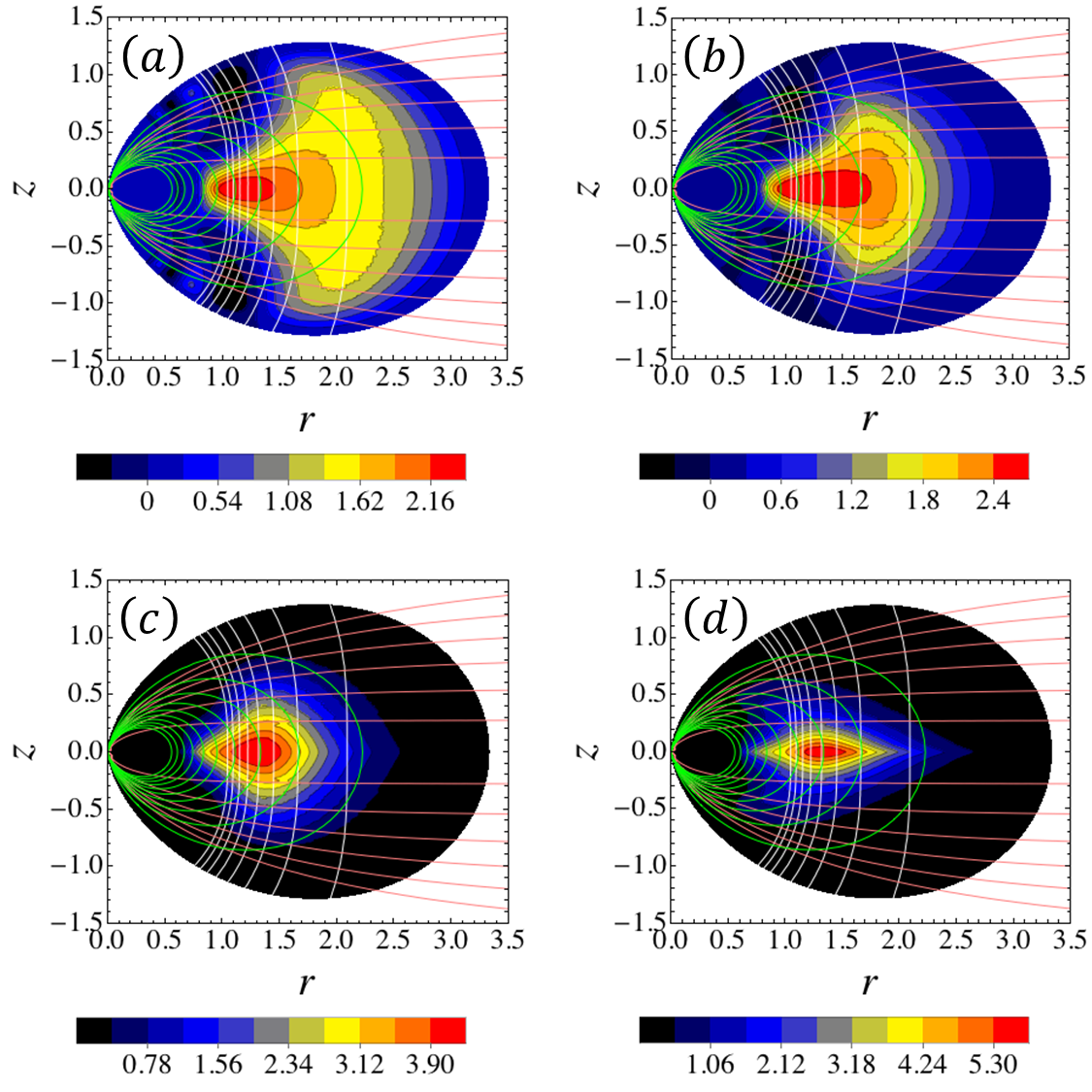
Figure 8: Normal diffusion dependence of the laboratory density $\rho$. (a): $10^{-2}D_{\perp}$ at $t=14.4$ and $\sim 84\%$ particles left. (b): $10^{-1}D_{\perp}$ at $t=7.2$ and $\sim 67\%$ particles left. (c): $D_{\perp}$ at $t=2.4$ and $\sim 55\%$ particles left. (d): $10D_{\perp}$ at $t=0.36$ and $\sim 46\%$ particles left. The status of total particle number $N_{tot}$ can be understood by comparing figure 2.

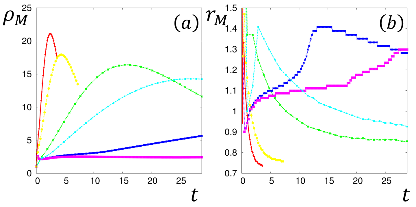
Figure 9: (a): time evolution of the instantaneous laboratory density maximum $\rho_{M}$. (b): time evolution of the density maximum radial position $r_{M}$. The color legend is identical to that of figure 2.

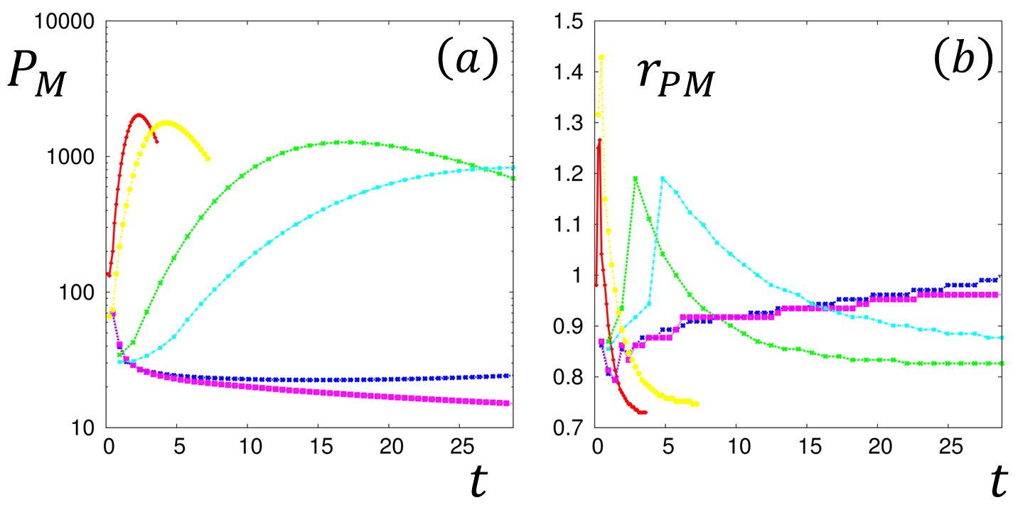
Figure 10: (a): time evolution of the instantaneous parallel pressure maximum $P_{M}$. (b): time evolution of the parallel pressure maximum radial position $r_{PM}$. The color legend is identical to that of figure 2.

VIII Conclusion

We have derived a model of the inward diffusion of magnetized particles across flux surfaces in magnetospheric plasmas. At the core of the formulation is the entropy principle on the symplectic submanifold of the macroscopic hierarchy that coarse-grains the microscopic action-angle variables (the magnetic moment and the gyro-angle). Modeling a random electric field of electrostatic turbulence by a Wiener process, the diffusion operator $\mathfrak{C}$ has been derived by careful application of stochastic analysis; the form of $\mathfrak{C}$ is considerably complicated including the geometry factor $\mathfrak{q}$ and the phase factor $\alpha$ of stochastic integral.

The geometry factor is due to the anisotropic motion of particles on non-orthogonal coordinates. When a particle experiences a jump in $\psi$, a simultaneous change in $\ell$ occurs. This coupling (scaled by $\mathfrak{q}$) yields the diffusion and drift terms in the parallel equation of motion; the latter is multiplied by $(1/2-\alpha)$. Putting $\alpha=0$ (Ito’s integral) retains the drift term, while putting $\alpha=1/2$ (Stratonovich’s integral) removes it. Since the drift term is due to the direct jumps in $\ell$ (not in $\dot{\ell}$), caused by the $E\times B$ drift motion in $x_{\perp}$, we conclude that $\alpha=0$ is the right choice (unlike the usual argument of employing Stratonovich’s integral for Brownian motion driven by jumps in velocities). Then, the drift term in (24) pushes particles back to the horizontal plane.

In the Fokker-Planck equation built in Sec. VI, we did not consider a dissipation mechanism acting in the direction perpendicular to flux-surfaces. Hence, particles can be heated by the random electric field, i.e., the system of particles is an open system. This makes the “asymptotic form” of the particle distribution somewhat different from those predicted by statistical equilibrium models. For example, the most simple model assumes that the third adiabatic invariant $\psi$ is most fragile, thus the relaxation will tend $\partial_{\psi}f(t\rightarrow\infty)\rightarrow 0$ Has . Or, assuming a grand canonical ensemble determined by the energy and magnetization, a Boltzmann distribution on the foliated (macroscopic) phase space can be derived YosFol , in which $f$ does not depend directly on $\psi$ (however, indirect dependence occurs though $B(\psi,\ell)$ in the Hamiltonian of magnetized particles). In the present model, we observe

$$\frac{\partial f}{\partial\psi}\left(t\rightarrow\infty\right)\neq 0,$$ (38)

which is apparent in (32)), as well as in the results of numerical simulations. Nevertheless, the diffusion term tends to diminish the gradient with respect to $\psi$.

IX Acknowledgements

The authors would like to acknowledge the useful advices provided by Y. Kawazura with numerical simulations.

Appendix A Analytical Expression of Point Dipole Field Line Length

We may measure the length $\ell$ of a field line $\tilde{\psi}$ either from the inside of the point dipole $(r,z)_{\ell=0}=(0,0)$, or from the outside $(r,z)_{\ell=0}=(\{\tilde{r}:\tilde{\psi}=\psi(\tilde{r},0)\},0)$.
Let us first derive the expression $\ell_{in}(r,z)$ corresponding to the first definition. We start by inverting the expression for $\psi(r,z)$ in order to obtain $z(r,\psi)$:

$$z^{2}=r^{\frac{3}{4}}\psi^{-\frac{2}{3}}-r^{2}.$$ (39)

Note that we are working with normalized quantities, i.e. $\psi=\psi^{*}/B_{0}L_{0}^{2}$, $z=z^{*}/L_{0}$ and $r=r^{*}/L_{0}$ where $B_{0}$ is the characteristic magnetic field, $L_{0}$ the characteristic length and the $*$ symbol indicates physical dimensions.

Since the stream function $\psi$ is constant along a field line, differentiation gives:

$$\frac{dz}{dr}=\pm\frac{\frac{2}{3}r^{\frac{1}{3}}\psi^{-\frac{2}{3}}-r}{\sqrt{r^{\frac{4}{3}}\psi^{-\frac{2}{3}}-r^{2}}}.$$ (40)

The desired length is then:

$$\ell_{in}(r,z)=\int_{0}^{r}{d\ell}=\int_{0}^{r}{\sqrt{\left(1+\left(\frac{dz}{dr}\right)^{2}\right)}dr}=\int_{0}^{r}{\sqrt{\frac{\frac{4}{9}\psi^{-\frac{4}{3}}-\frac{1}{3}r^{\frac{2}{3}}\psi^{-\frac{2}{3}}}{r^{\frac{2}{3}}\psi^{-\frac{2}{3}}-r^{\frac{4}{3}}}}dr}.$$ (41)

To evaluate this integral we perform the change of variable $x=(r\psi)^{\frac{2}{3}}$. This gives:

$$\ell_{in}(r,z)=\frac{1}{2\psi}\int_{0}^{(r\psi)^{\frac{2}{3}}}{\sqrt{\frac{4-3x}{1-x}}}dx=\frac{1}{2\psi}\int_{0}^{(r\psi)^{\frac{2}{3}}}{\frac{1+4-3x+3-3x}{2\sqrt{1-x}\sqrt{4-3x}}}dx=\frac{1}{2\psi}\int_{0}^{(r\psi)^{\frac{2}{3}}}{\left(\frac{1}{2\sqrt{1-x}\sqrt{4-3x}}+\frac{\sqrt{4-3x}}{2\sqrt{1-x}}+\frac{3\sqrt{1-x}}{2\sqrt{4-3x}}\right)}dx=-\frac{1}{2\psi}{\left\{{\frac{\ln{\left[{3\sqrt{1-x}+\sqrt{12-9x}}\right]}}{\sqrt{3}}+\sqrt{1-x}\sqrt{4-3x}}\right\}}_{0}^{(r\psi)^{2/3}}=\frac{1}{2\psi}\left[2-\frac{1}{\sqrt{3}}\ln\left(\frac{\sqrt{3}\sqrt{1-(r\psi)^{\frac{2}{3}}}+\sqrt{4-3(r\psi)^{\frac{2}{3}}}}{2+\sqrt{3}}\right)-\sqrt{1-(r\psi)^{\frac{2}{3}}}\sqrt{4-3(r\psi)^{\frac{2}{3}}}\right].$$ (42)

Here $\psi=\psi(r,z)=\frac{r^{2}}{(r^{2}+z^{2})^{3/2}}$. In a similar manner, it can be shown that the expression for the field line length as measured from the outside of the dipole is:

$$\ell_{out}(r,z)=\int_{\tilde{r}}^{r}{d\ell}=\frac{1}{2\psi}\left[\frac{1}{\sqrt{3}}\ln\left(\sqrt{3}\sqrt{1-(r\psi)^{\frac{2}{3}}}+\sqrt{4-3(r\psi)^{\frac{2}{3}}}\right)\\ +\sqrt{1-(r\psi)^{\frac{2}{3}}}\sqrt{4-3(r\psi)^{\frac{2}{3}}}\right].$$ (43)

Appendix B Change of Variables (Ito’s Lemma)

Theorem B.1

Define the stochastic integral of a real-valued function $g$ as

$$\int_{s}^{r}gdW=ms\text{-}\lim_{n\to\infty}\sum_{i=1}^{n}g(t_{i-1}+\alpha\Delta t_{i})[W(t_{i})-W(t_{i-1})],$$ (44)

with $\alpha\in[0,1]$. Let $X(\cdot)$ be a real-valued stochastic process satisfying

$$X(r)=X(s)+\int_{s}^{r}Fdt+\int_{s}^{r}G_{\alpha}dW,$$ (45)

with $F\in L^{1}(0,T)$, $G\in L^{2}(0,T)$ and $0\leq s\leq r\leq T$. Consider a new stochastic process $Y=y(X(t),t)$, where $y:\mathbb{R}\times[0,T]\rightarrow\mathbb{R}$ and $y\in C^{2}$ on its domain. Then $Y$ has the stochastic differential:

$$dY(X,t)=\frac{\partial y}{\partial t}dt+\frac{\partial y}{\partial x}dX+\left(\frac{1}{2}-\alpha\right)G^{2}\frac{\partial^{2}y}{\partial x^{2}}dt=\left(\frac{\partial y}{\partial t}+F\frac{\partial y}{\partial x}+\left(\frac{1}{2}-\alpha\right)G^{2}\frac{\partial^{2}y}{\partial x^{2}}\right)dt+G_{\alpha}\left(\frac{\partial y}{\partial x}\right)_{\alpha}dW,$$ (46)

where, as usual, the subscript $\alpha$ indicates evaluation at $t_{\alpha}=t_{i-1}+\alpha\Delta t_{i}$.

Ito’s lemma can be obtained by putting $\alpha=0$. Stratonovich’s definition comes instead from the choice $\alpha=1/2$. It is interesting to see that in this case the stochastic chain rule has the same form of the chain rule of classic calculus. Physically this is because the Stratonovich interpretation, as we showed in chapter $4$, describes processes with a continuous variation in time.

A rigorous proof of the theorem can be obtained by following that given in Evans for the case $\alpha=0$. For the seek of simplicity we give below an informal proof based on Taylor expansion.

Proof

We proceed by Taylor expansion around $t_{i-1}$ and retain only terms of order $dt$:

$$dY(X,t)=\frac{\partial y}{\partial t}dt+\frac{\partial y}{\partial x}dX+\frac{1}{2}\frac{\partial^{2}y}{\partial x^{2}}dX^{2}+...=\frac{\partial y}{\partial t}dt+\frac{\partial y}{\partial x}Fdt+\left(\frac{\partial y}{\partial x}\right)_{i-1}G_{\alpha}dW+\frac{1}{2}\left(\frac{\partial^{2}y}{\partial x^{2}}\right)_{i-1}G^{2}_{\alpha}dW^{2}+...=\frac{\partial y}{\partial t}dt+\frac{\partial y}{\partial x}Fdt+\left(\left(\frac{\partial y}{\partial x}\right)_{\alpha}-\left(\frac{\partial^{2}y}{\partial x^{2}}\right)_{\alpha}(X_{\alpha}-X_{i-1})\right)G_{\alpha}dW+\frac{1}{2}\left(\frac{\partial^{2}y}{\partial x^{2}}\right)_{\alpha}G^{2}_{\alpha}dW^{2}+...=\frac{\partial y}{\partial t}dt+\frac{\partial y}{\partial x}Fdt+\left(\frac{\partial y}{\partial x}\right)_{\alpha}G_{\alpha}dW+\left(\frac{\partial^{2}y}{\partial x^{2}}\right)_{\alpha}\left(\frac{dW^{2}}{2}-dW_{\alpha}dW\right)G^{2}_{\alpha}+...=\left(\frac{\partial y}{\partial t}+F\frac{\partial y}{\partial x}+\left(\frac{1}{2}-\alpha\right)G^{2}\frac{\partial^{2}y}{\partial x^{2}}\right)dt+\left(\frac{\partial y}{\partial x}\right)_{\alpha}G_{\alpha}dW+O(dt^{3/2}).$$ (47)

Here we used the fact that

$$\langle dW_{\alpha}dW\rangle=\langle(W_{\alpha}-W_{i-1})(W_{i}-W_{i-1})\rangle=\alpha\Delta t_{i},$$ (48)

and deduced the heuristic formula $dW_{\alpha}dW\sim\alpha dt$. $\blacksquare$

Appendix C Stochastic Integral

Theorem C.1

Define the stochastic integral of a real-valued function $g$ as

$$\int_{s}^{r}gdW=ms\text{-}\lim_{n\to\infty}\sum_{i=1}^{n}g(t_{i-1}+\alpha\Delta t_{i})[W(t_{i})-W(t_{i-1})],$$ (49)

with $\alpha\in[0,1]$. Let $f=f(X,t)$ be a real-valued function of a random process $X(\cdot)$ satisfying

$$X(r)=X(s)+\int_{s}^{r}Fdt+\int_{s}^{r}GdW,$$ (50)

where the integral is in the Ito sense $\alpha=0$, $F\in L^{1}(0,T)$, $G\in L^{2}(0,T)$ and $0\leq s\leq r\leq T$. Then, the following relation holds:

$$(df)_{Ito}=(df)_{\alpha}-\alpha\frac{\partial f}{\partial x}\frac{\partial G}{\partial x}Gdt.$$ (51)

What theorem $1$ tells us is that integrating $df$ with Ito’s definition $\alpha=0$ is equivalent to integrating $df$ with a generic $\alpha$ definition, provided that we add the correction factor $-\alpha\frac{\partial f}{\partial x}\frac{\partial G}{\partial x}Gdt$.

Proof

The first step will be to find the expression of a stochastic differential equation in the Ito sense in terms of a stochastic differential equation equipped with a generic $\alpha$ definition of the stochastic integral. To accomplish this, consider the Ito SDE

$$dX_{I}=Fdt+G_{i-1}dW,$$ (52)

where the subscript $I$ indicates Ito’s definition $\alpha=0$ of the stochastic integral and $i-1$ the fact that the function $G$ is evaluated at the left point $t_{i-1}$ of the time interval $\Delta t_{i}=t_{i}-t_{i-1}$. If we expand $G_{i-1}$ at first order in $dt$ around $t_{\alpha}=t_{i-1}+\alpha\Delta t_{i}$ with $\alpha\in[0,1]$, we have

$$dX_{I}=Fdt+\left(G_{\alpha}+\left(\frac{\partial G}{\partial x}\right)_{\alpha}(X_{i-1}-X_{\alpha})-\alpha\left(\frac{\partial G}{\partial t}\right)_{\alpha}\Delta t_{i}\right)dW+...=Fdt+\left(G_{\alpha}-\left(\frac{\partial G}{\partial x}\right)_{\alpha}(\alpha F\Delta t_{i}+G_{i-1}dW_{\alpha})\right)dW+...=Fdt+G_{\alpha}dW-\left(\frac{\partial G}{\partial x}\right)_{\alpha}G_{\alpha}dW_{\alpha}dW+...\quad.$$ (53)

Here the subscript $\alpha$ indicates evaluation at point $t_{\alpha}$. Now note that

$$\langle dW_{\alpha}dW\rangle=\langle(W_{\alpha}-W_{i-1})(W_{i}-W_{i-1})\rangle=\alpha\Delta t_{i}.$$ (54)

We conclude that

$$dX_{I}=\left[F-\alpha\left(\frac{\partial G}{\partial x}\right)G\right]dt+G_{\alpha}dW+O(dt^{3/2}).$$ (55)

Note that for the terms proportional to $dt$ the choice of $\alpha$ is irrelevant since they correspond to Riemann integration. Equation (55) is the stochastic differential equation in terms of a generic $\alpha$-integral corresponding to the stochastic differential equation in the Ito sense (52).

We are now ready to prove the main result. Using again Taylor expansion around $t_{\alpha}$ and retaining only terms of order $dt$, we have

$$(df)_{I}=\frac{\partial f}{\partial t}dt+\frac{\partial f}{\partial x}dX_{I}+\frac{1}{2}\frac{\partial^{2}f}{\partial x^{2}}dX_{I}^{2}+...=\frac{\partial f}{\partial t}dt+\frac{\partial f}{\partial x}Fdt+\left(\frac{\partial f}{\partial x}\right)_{i-1}G_{i-1}dW+\frac{1}{2}\frac{\partial^{2}f}{\partial x^{2}}(G_{i-1}^{2}dW^{2})+...=\left(\frac{\partial f}{\partial t}+\frac{\partial f}{\partial x}F+\frac{1}{2}\frac{\partial^{2}f}{\partial x^{2}}G^{2}\right)dt+\left(\left(\frac{\partial f}{\partial x}\right)_{\alpha}+\left(\frac{\partial^{2}f}{\partial x^{2}}\right)_{\alpha}(X_{i-1}-X_{\alpha})\right)\left(G_{\alpha}+\left(\frac{\partial G}{\partial x}\right)_{\alpha}(X_{i-1}-X_{\alpha})\right)dW+...=\left(\frac{\partial f}{\partial t}+\frac{\partial f}{\partial x}F+\frac{1}{2}\frac{\partial^{2}f}{\partial x^{2}}G^{2}\right)dt+\left(\frac{\partial f}{\partial x}\right)_{\alpha}G_{\alpha}dW-\left(\frac{\partial f}{\partial x}\right)_{\alpha}\left(\frac{\partial G}{\partial x}\right)_{\alpha}G_{\alpha}dW_{\alpha}dW-\left(\frac{\partial^{2}f}{\partial x^{2}}\right)_{\alpha}G^{2}_{\alpha}dW_{\alpha}dW+...=\left(\frac{\partial f}{\partial t}+\frac{\partial f}{\partial x}F+\left(\frac{1}{2}-\alpha\right)\frac{\partial^{2}f}{\partial x^{2}}G^{2}-\alpha\frac{\partial f}{\partial x}\frac{\partial G}{\partial x}G\right)dt+\left(\frac{\partial f}{\partial x}\right)_{\alpha}G_{\alpha}dW+...=(df)_{\alpha}-\alpha\frac{\partial f}{\partial x}\frac{\partial G}{\partial x}Gdt+O(dt^{3/2}).$$ (56)

Here we used the generalized Ito’s lemma (46) obtained in appendix B to identify $(df)_{\alpha}$. $\blacksquare$

Note that when $G$ is constant $(df)_{I}=(df)_{\alpha}$.

Appendix D The $\ell$-Equation

Since $\ell$ is a function of $x_{\perp}$, when evaluating how $\ell$ is affected by a random change in $x_{\perp}$ Ito’s lemma (46) has to be applied accordingly. Recalling (9), we have

$$(dL)_{turbulence}=\left(\frac{1}{2}-\alpha\right)\frac{D_{\perp}}{(rB)^{2}}\frac{\partial^{2}\ell}{\partial x_{\perp}^{2}}dt+\mathfrak{q}D_{\perp}^{1/2}dW_{\perp}=\left(\frac{1}{2}-\alpha\right)\frac{D_{\perp}}{(rB)^{2}}\frac{\partial}{\partial x_{\perp}}\left(\mathfrak{q}rB\right)+\mathfrak{q}D_{\perp}^{1/2}dW_{\perp}=\left(\frac{1}{2}-\alpha\right)\frac{D_{\perp}}{rB}\left(\mathfrak{q}\frac{\partial}{\partial\ell}+\frac{\partial}{\partial\psi}\right)\left(\mathfrak{q}rB\right)+\mathfrak{q}D_{\perp}^{1/2}dW_{\perp}=\left(\frac{1}{2}-\alpha\right)D_{\perp}\left[\left(\mathfrak{q}\frac{\partial}{\partial\ell}+\frac{\partial}{\partial\psi}\right)\mathfrak{q}+\mathfrak{q}\left(\mathfrak{q}\frac{\partial}{\partial\ell}+\frac{\partial}{\partial\psi}\right)\ln(rB)\right]dt+\mathfrak{q}D_{\perp}^{1/2}dW_{\perp},$$ (57)

where the following relationship was used:

$$\begin{split}\partial_{\perp}&=\frac{\partial}{\partial x_{\perp}}=\frac{\partial\ell}{\partial x_{\perp}}\frac{\partial}{\partial\ell}+\frac{\partial\psi}{\partial x_{\perp}}\frac{\partial}{\partial\psi}\\ =&\nabla\ell\cdot\partial_{\perp}\partial_{\ell}+rB\partial_{\psi}=rB\left(\mathfrak{q}\partial_{\ell}+\partial_{\psi}\right).\end{split}$$ (58)

Taking into account $v_{\parallel}$ gives (13).

References

- (1) J. W. Warwick et al., 1981, Planetary Radio Astronomy Observations From Voyager 1 Near Saturn, Science 212, 239 ?243
- (2) F. L. Scarf, D. A. Gurnett, W. S. Kurth, and R. L. Poynter, 1982, Voyager 2 Plasma Wave Observations at Saturn, Science, Vol. 215 no. 4532 pp. 587-594
- (3) D. A. Gurnett et al., 2004, The Cassini Radio and Plasma Wave Investigation, Space Science Reviews 114: 395 ?463
- (4) Z. Yoshida, H. Saitoh, J. Morikawa, Y. Yano, S. Watanabe, and Y. Ogawa, 2010, Magnetospheric vortex formation: self-organized confinement of charged particles, Phys. Rev. Lett. 104 235004 1-4
- (5) A. C. Boxer, R. Bergmann, J. L. Ellsworth, D. T. Garnier, J. Kesner, M. E. Mauel, and P. Woskov, 2010, Turbulent inward pinch of plasma confined by a levitated dipole magnet, Nature Physics, Vol 6, 207-212
- (6) C. G. Falthammar, 1965, Effects of Time-Dependent Electric Fields on Geomagnetically Trapped Radiation, J. of Geophys. Res., Vol. 70, No. 11
- (7) T. J. Birmingham, T. G. Northrop, and C. G. Falthammar, 1967, Charged Particle Diffusion by Violation of the Third Adiabatic Invariant, The Physics of Fluids, Vol. 10, No. 11
- (8) J. M. Cornwall, 1972, Radial Diffusion of Ionized Helium and Protons: A Probe for Magnetospheric Dynamics, J. Geophys. Res., Vol. 77, No. 10
- (9) W. N. Spjeldvik, 1996, Cross Field Entry of High Charge State Energetic Heavy Ions into the Earth’s Magnetosphere, Radiation Belts: Models and Standards, Geophysical Monograph 97, p. 63,the American Geophysical Union
- (10) M. C. Fok, T. E. Moore, and W. N. Spjeldvik, et al., March 1 2001, Rapid enhancement of radiation belt electron fluxes due to substorm dipolarization of the geomagnetic field, J. Geophys. Res., Vol. 106, No. A3, Pages 3873-3881
- (11) Y. Zheng, M. C. Fok, and G. V. Khazanov, 2003, A radiation belt-ring current forecasting model, Space Weather, Vol. 1, No. 3, 1013
- (12) M. C. Fok and T. E. Moore, 1997, Ring current modeling in a realistic magnetic field configuration, Geophys. Res. Lett., Vol. 24, No. 14, Pages 1775-1778
- (13) M. C. Fok, R. B. Horne, N. P. Meredith, and S. A. Glauert, 2008, Radiation Belt Environment model: application to space weather nowcasting, J. Geophys. Res., Vol. 113, A03S08
- (14) A. M. Persoon, D. A. Gurnett, W. S. Kurth, G. B. Hospodarsky, J. B. Groene, P. Canu, and M. K. Dougherty, 2005, Equatorial electron density measurements in Saturn’s inner magnetosphere, Geophys. Res. Lett., Vol. 32, L23105
- (15) A. M. Persoon et al., 2009, A diffusive equilibrium model for the plasma density in Saturn’s magnetosphere, J. Geophys. Res., Vol. 114, A04211
- (16) A. M. Persoon et al., 2013, The plasma density distribution in the inner region of Saturn’s magnetosphere, J. Geophys. Res.: Space Phys., Vol. 118, 2970-2974
- (17) J. D. Richardson and E. C. Sittler, 1990, A Plasma Density Model For Saturn Based On Voyager Observations, J. Geophys. Res., Vol. 95, No. A8, 12019-12031
- (18) J. D. Richardson, 1995, An extended plasma model for Saturn, Geophys. Res. Lett., Vol. 22, No. 10, 1177-1180
- (19) A. Hasegawa, 2005, Motion of a charged particle and plasma equilibrium in a dipole magnetic field-can a magnetic field trap a charged particle? Can a magnetic field having bad curvature trap a plasma stably?, Phys. Scr. T 116 72-74
- (20) P. Schippers, M. Moncuquet, N. Meyer-Vernet, and A. Lecacheux, 2013, Core electron temperature and density in the innermost Saturn’s magnetosphere from HF power spectra analysis on Cassini, J. Geophys. Res.: Space Phys., Vol. 118, 7170-7180
- (21) Z. Yoshida and S. M. Mahajan, 2014, Self-Organization in Foliated Phase-Space: a Construction of Scale Hierarchy by Adiabatic Invariants of Magnetized Particles, Prog. Theor. Exp. Phys., 073J01
- (22) Z. Yoshida and P. J. Morrison, 2014, Unfreezing Casimir invariants: singular perturbations giving rise to forbidden instabilities, in Nonlinear physical systems: spectral analysis, stability and bifurcation, Ed. by O. N. Kirillov and D. E. Pelinovsky, (ISTE and John Wiley and Sons) Chap. 18, pp. 401–419.
- (23) Z. Yoshida and P. J. Morrison, 2014, A hierarchy of noncanonical Hamiltonian systems: circulation laws in an extended phase space, Fluid Dyn. Res. 46, 031412 1–21.
- (24) Z. Yoshida et al., 2013, Self-organized confinement by magnetic dipole: recent results from RT-1 and theoretical modeling, Plasma Phys. Control. Fusion 55, 014018
- (25) H. Saitoh, Y. Yano, Z. Yoshida, M. Nishiura, J. Morikawa, Y. Kawazura, T. Nogami and M. Yamasaki, 2014, Observation of a new high- and high-density state of a magnetospheric plasma in RT-1, Phys. Plasmas 21, 082511 1–6.
- (26) J. R. Cary and A. J. Brizard, 2009, Hamiltonian theory of guiding-center motion, Rev. Mod. Phys. 81, 693
- (27) C. W. Gardiner, 1985, Handbook of Stochastic Methods for Physics, Chemistry and the Natural Sciences, 2nd edition, (Springer-Verlag)
- (28) H. Risken, 1989, The Fokker-Planck Equation. Methods of Solution and Applications, 2nd edition, (Springer-Verlag)
- (29) L. C. Evans, 2014, An Introduction to Stochastic Differential Equations, (American Mathematical Society)
- (30) I. I. Eliazar and M. F. Shlesinger, 2013, Fractional Motions, Physics Reports 527 101-129
- (31) E. Wong and M. Zakai, 1965, On The Convergence of Ordinary Integrals to Stochastic Integrals, Ann. Math. Stat., Vol. 36, No. 5, 1560-1564
- (32) N. G. van Kampen, 1981, Ito Versus Stratonovich, J. Stat. Phys., Vol. 24, No. 1
- (33) N. G. van Kampen, 1981, The Validity of Nonlinear Langevin Equations, J. Stat. Phys, Vol. 25, No. 3
- (34) T. Kuroiwa and K. Miyazaki, 2014, Brownian Motion With Multiplicative Noises Revisited, J. Phys. A: Math. Theor. 47
- (35) W. Moon and J. S. Wettlaufer, 2014, On the Interpretation of Stratonovich Calculus, New J. Phys 16 055017
- (36) J. M. Sancho, 2011, Brownian colloidal particles: Ito, Stratonovich, or a different stochastic interpretation, Physical Review E 84, 062102
- (37) A. Chechkin and I. Pavlyukevich, 2014, Marcus Versus Stratonovich for Systems With Jump Noise, J. Phys. A: Math. Theor. 47 342001
- (38) G. Ran and D. Jiulin, 2013, Power-Law Behaviors from the Two-Variable Langevin Equation: Ito’s and Stratonovich’s Fokker-Planck Equations, J. Stat. Mech.: Theor. Exp.
- (39) R. Yuan and P. Ao, 2012, Beyond Ito Versus Stratonovich, J. Stat. Mech.: Theor. Exp.
- (40) O. Farago and N. Gronbech-Jensen, 2014, Langevin Dynamics in Inhomogeneous Media: Re-Examining the Ito-Stratonovich Dilemma, Physical Review E 89, 013301
- (41) G. Volpe, L. Helden, T. Brettschneider, J. Wehr, and C. Bechinger, 2010, Influence of Noise on Force Measurements, Phys. Rev. Lett. 104 170602
- (42) R. Mannella and P. V. E. McClintock, 2011, Comment on ‘Influence of Noise on Force Measurements’, PRL 107, 078901
- (43) A. W. C. Lau, T. C. Lubensky, 2007, State-Dependemt Diffusion: Thermodynamic Consistency and its Path Integral Formulation, Phys. Rev. E 76, 011123
- (44) K. Ito, 1944, Stochastic Integral, Proc. Imp. Acad., Vol. 20, Number 8, 519-524
- (45) K. Ito, 1950, Stochastic Differential Equations in a Differentiable Manifold, Nagoya Math. J. Volume 1, 35-47
- (46) K. Ito, 1951, On a Formula Concerning Stochastic Differentials, Nagoya Math. J. Volume 3, 55-65