Irreducible background and interference effects for Higgs-boson production in association with a top-quark pair

Abstract

We present an analysis of Higgs-boson production in association with a top-quark pair at the LHC investigating in particular the final state consisting of four b jets, two jets, one identified charged lepton and missing energy. We consider the Standard Model prediction in three scenarios, the resonant Higgs-boson plus top-quark-pair production, the resonant production of a top-quark pair in association with a b-jet pair and the full process including all non-resonant and interference contributions. By comparing these scenarios we examine the irreducible background for the production rate and several kinematical distributions. With standard selection criteria the irreducible background turns out to be three times as large as the signal. For most observables we find a uniform deviation of eight percent between the scenario requiring two resonant top quarks and the full process. In particular phase-space regions the non-resonant contributions cause larger effects, and we observe shape changes for some distributions. Furthermore we investigate interference effects and find that neglecting interference contributions results in an over-estimate of the total cross-section of five percent.

1 Introduction

The discovery of the long-sought Higgs boson at the LHC in July 2012 Aad:2012tfa ; Chatrchyan:2012ufa ushered in a new era of probing the mechanism of spontaneous symmetry breaking and thus mass generation in nature. The determination of the properties of the discovered Higgs boson is a major goal of the LHC. Especially the couplings of the Higgs boson to matter particles are important for the understanding of the origin of mass. The production of a Higgs boson in association with a top-quark pair is of particular interest, since it allows to directly access the top-quark Yukawa coupling. Although the production rate is small and the measurement is experimentally challenging, ATLAS ATLAS:2012cpa ; ATLAS:2014 ; Aad:2014lma and CMS CMS:2012qaa ; CMS:2013sea ; CMS-PAS-HIG-13-015 ; Chatrchyan:2013yea ; Khachatryan:2014qaa have already performed searches using the data of the LHC runs at 7 and $8\,\text{TeV}$. With the upcoming run 2 of the LHC at $13\,\text{TeV}$ the determination of the $\text{t}\bar{\text{t}}\text{H}$ signal and the potential measurement of the top-quark Yukawa coupling will be pursued.

The production of a Higgs boson in association with a top–antitop pair has been studied theoretically by many authors. Leading-order (LO) predictions for the production of $\text{t}\bar{}\text{t}\text{H}$ for stable Higgs boson and top quarks have been presented in Refs. Raitio:1978pt ; Ng:1983jm ; Kunszt:1984ri ; Gunion:1991kg ; Marciano:1991qq while the corresponding next-to-leading-order (NLO) corrections have been calculated in Refs. Beenakker:2001rj ; Beenakker:2002nc ; Reina:2001sf ; Dawson:2002tg ; Dawson:2003zu . More recently the matching of the NLO corrections to parton showers has been performed Frederix:2011zi ; Garzelli:2011vp . Very recently also electroweak corrections to $\text{t}\bar{}\text{t}\text{H}$ have been elaborated Frixione:2014qaa ; Yu:2014cka . NLO QCD corrections for the most important irreducible background process, $\text{t}\bar{}\text{t}\text{b}\bar{}\text{b}$ production in LO QCD, have been worked out Bredenstein:2008zb ; Bredenstein:2009aj ; Bevilacqua:2009zn ; Bredenstein:2010rs and matched to parton showers Kardos:2013vxa ; Cascioli:2013era ; TROCSANYI:2014lha . A combined analysis of $\text{t}\bar{}\text{t}\text{H}$ and $\text{t}\bar{}\text{t}\text{b}\bar{}\text{b}$ production was carried out in Ref. Binoth:2010ra . Further analyses and results can be found in the yellow reports of the LHC Higgs Cross Section Working Group Dittmaier:2011ti ; Dittmaier:2012vm ; Heinemeyer:2013tqa .

In this article we study Higgs-boson production in association with a top-quark pair ($\text{t}\bar{\text{t}}\text{H}$) including the subsequent semileptonic decay of the top-quark pair and the decay of the Higgs boson into a bottom–antibottom-quark pair,

$$\text{p}\text{p}\to\text{t}\bar{\text{t}}\text{H}\to\ell^{+}\nu_{\ell}\text{j}\text{j}\text{b}\bar{\text{b}}\text{b}\bar{\text{b}}.$$ (1)

The final state under consideration consists of six jets, four of which are b jets, one identified charged lepton (electron or muon) and missing energy, and our primary goal is the study of the irreducible background. We consider this process in three different scenarios. In the first scenario we include the complete Standard Model (SM) contributions, comprising all resonant, non-resonant and interference contributions to the 8-particle final state. For the second scenario we require the intermediate resonant production of a top-quark pair in association with a bottom-quark pair. We employ the pole approximation for the top quarks and include the leptonic/hadronic decay of the top/antitop quark. Similar approaches have been used for $\text{t}\bar{\text{t}}$ production in association with massless particles at NLO QCD Melnikov:2011ta ; Melnikov:2011qx . In the third scenario, corresponding to the signal, we require in addition to the resonant top-quark pair an intermediate resonant Higgs boson decaying into a bottom-quark pair and employ the pole approximation for the Higgs boson as well. We use the matrix-element generator RECOLA Actis:2012qn to compute all matrix elements at leading order in perturbation theory.

Comparing the predictions in the three scenarios allows us to examine the size of the irreducible background for Higgs production in association with a top–antitop-quark pair. Further we determine the quality of the approximations compared to the calculation of the full process and quantify deviations for the total cross section and differential distributions. We investigate the total cross section and differential distributions for the LHC operating at $13\,\text{TeV}$ with particular emphasis on distributions that allow to enhance the signal over the irreducible background. We study, in particular, different methods of assigning a b-jet pair to the Higgs boson and compare their performance in reconstructing the Higgs signal. Furthermore, we investigate the size of interference effects between contributions to the matrix elements of different order in the strong and electroweak coupling constants.

The paper is organised as follows. In Section 2 we specify the setup of our calculation and identify the various partonic contributions to the signal process. In Section 3 we present numerical results for the total cross section and kinematical distributions and quantify the size of the irreducible background. Our conclusions are presented in Section 4. In Appendix A we explain in detail the on-shell projections needed for the pole approximations we apply and in Appendix B we present additional results.

2 Notation and setup

This section provides some technical details about our computation. We consider gluons and light (anti-)quarks ($\text{u},\text{d},\text{c},\text{s}$) to be the only constituents of the proton and disregard contributions from bottom quarks and photons in the parton distribution functions. We neglect flavour mixing as well as finite-mass effects for the light quarks and leptons. The considered matrix elements involve (multiple) resonances of electroweak gauge bosons, top quarks and the Higgs boson. For the consistent description of these resonances we use the complex-mass scheme Denner:1999gp ; Denner:2005fg ; Denner:2006ic where all masses of unstable particles are defined by the poles of the propagators in the complex plane, $\mu^{2}=m^{2}-\mathrm{i}m\Gamma$. In addition, all couplings, and, in particular the weak mixing angle, are consistently derived from the complex masses and thus are complex, too.

We consider three scenarios to calculate the process $\text{p}\text{p}\to\ell^{+}\nu_{\ell}\text{j}\text{j}\text{b}\bar{\text{b}}\text{b}\bar{\text{b}}$:

• In the first scenario, the full process, we include all SM contributions to the process $\text{p}\text{p}\to\ell^{+}\nu_{\ell}\text{j}\text{j}\text{b}\bar{\text{b}}\text{b}\bar{\text{b}}$. Counting u, d, c, and s quarks separately, we distinguish 48 partonic channels. Eight channels can be constructed from $\text{g}\text{g}\to\ell^{+}\nu_{\ell}q^{\prime}\bar{q}^{\prime\prime}\text{b}\bar{\text{b}}\text{b}\bar{\text{b}}$ and 40 from $q\bar{q}\to\ell^{+}\nu_{\ell}q^{\prime}\bar{q}^{\prime\prime}\text{b}\bar{\text{b}}\text{b}\bar{\text{b}}$ using crossing symmetries and substituting different quark flavours. Matrix elements involving external gluons receive contributions of $\mathcal{O}{\left(\alpha_{\text{s}}\alpha^{3}\right)}$, $\mathcal{O}{\left(\alpha_{\text{s}}^{2}\alpha^{2}\right)}$ and $\mathcal{O}{\left(\alpha_{\text{s}}^{3}\alpha\right)}$, whereas amplitudes without external gluons receive an additional $\mathcal{O}{\left(\alpha^{4}\right)}$ term of pure electroweak origin. Some sample diagrams are shown in Figures 1(a)–1(c).

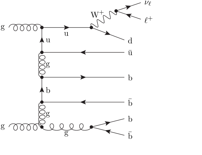
  (a)

  

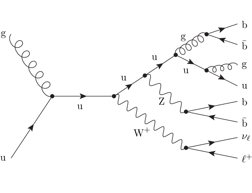
  (b)

  

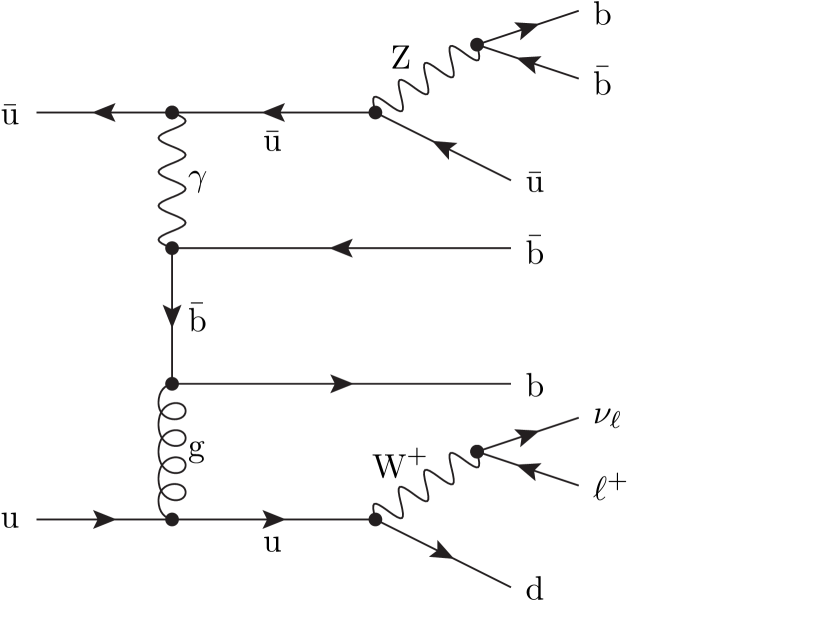
  (c)

  

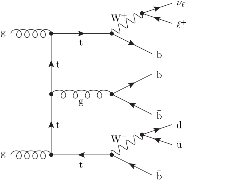
  (d)

  

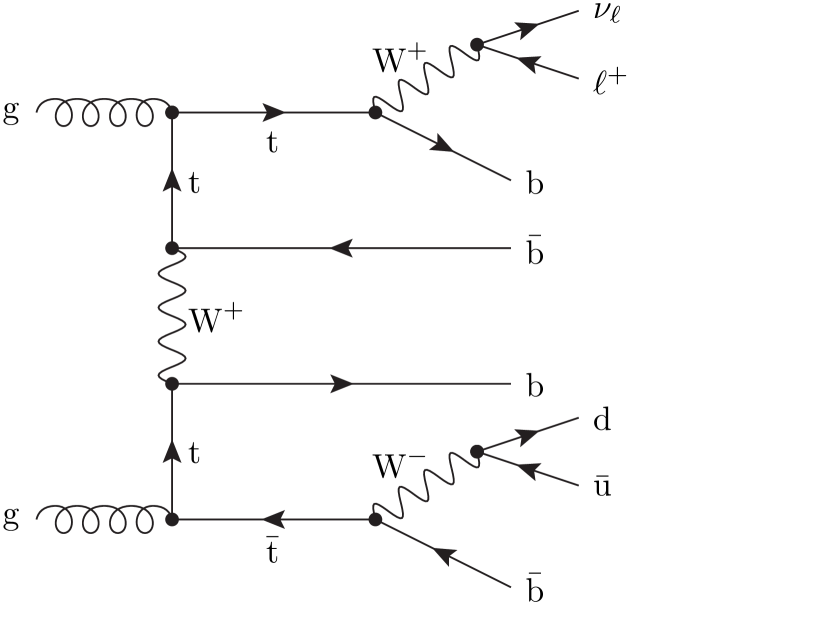
  (e)

  

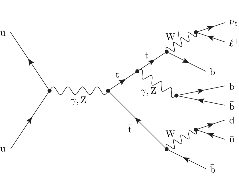
  (f)

  

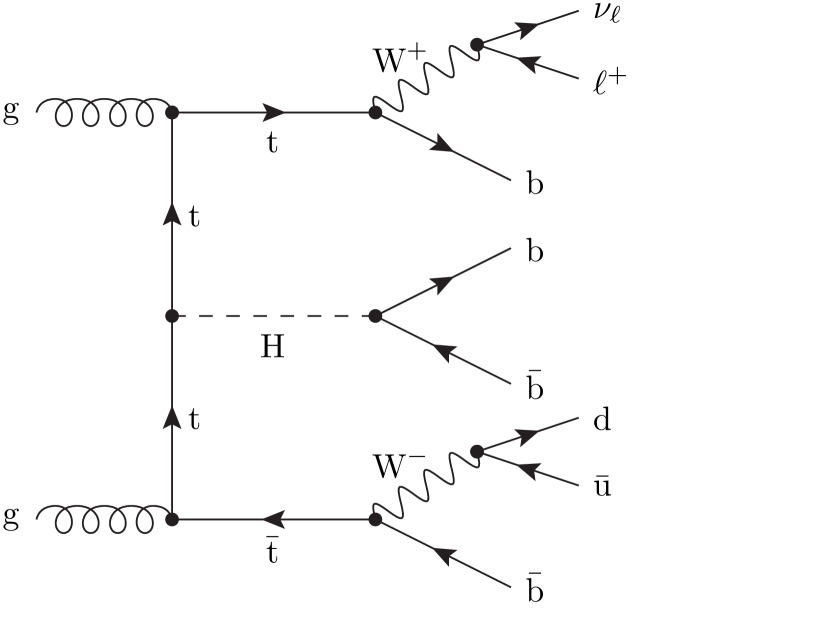
  (g)

  

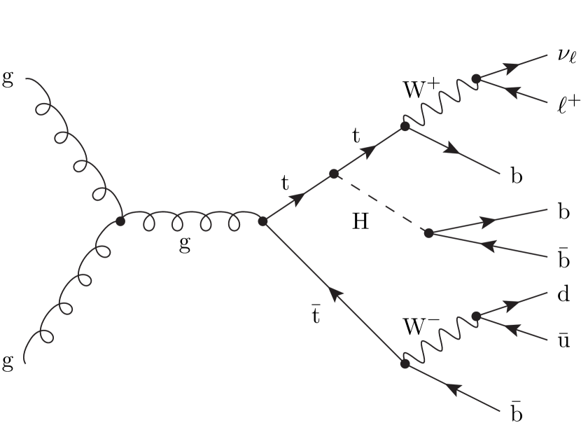
  (h)

  

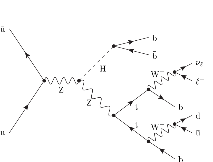
  (i)

  

  Figure 1: Representative Feynman diagrams for 1(a)–1(c) the full process (top), 1(d)–1(f) $\text{t}\bar{\text{t}}\text{b}\bar{\text{b}}$ production (middle) and 1(g)–1(i) $\text{t}\bar{\text{t}}\text{H}$ production (bottom).

• In the second scenario we only take those diagrams into account that contain an intermediate top–antitop-quark pair. The resulting amplitude, labelled $\text{t}\bar{\text{t}}\text{b}\bar{\text{b}}$ production in the following, corresponds to the production of a bottom–antibottom pair and an intermediate top–antitop pair followed by its semileptonic decay, i.e. $\text{p}\text{p}\to\text{t}\bar{\text{t}}\text{b}\bar{\text{b}}\to\ell^{+}\nu_{\ell}\text{j}\text{j}\text{b}\bar{\text{b}}\text{b}\bar{\text{b}}$. Some sample diagrams are shown in Figures 1(d)–1(f). Note that we use the pole approximation for the top quarks only, hence we take into account all off-shell effects of the remaining unstable particles. The details of our implementation of the pole approximation are described in Appendix A. This scenario involves 10 partonic channels, comprising 2 gluon-fusion and 8 quark–antiquark-annihilation channels. As a consequence of the required top–antitop-quark pair the amplitudes receive no contribution of $\mathcal{O}{\left(\alpha_{\text{s}}^{3}\alpha\right)}$.

• Finally, we consider the signal process $\text{p}\text{p}\to\text{t}\bar{\text{t}}\text{H}\to\ell^{+}\nu_{\ell}\text{j}\text{j}\text{b}\bar{\text{b}}\text{b}\bar{\text{b}}$ and label it $\text{t}\bar{\text{t}}\text{H}$ production. In addition to the intermediate top–antitop-quark pair we require an intermediate Higgs boson decaying into a bottom–antibottom-quark pair and use the pole approximation for the top-quark pair and the Higgs boson. Here the same 10 partonic channels as in the previous case contribute. The requirement of the Higgs boson eliminates contributions of the $\mathcal{O}{\left(\alpha_{\text{s}}^{2}\alpha^{2}\right)}$ from the amplitude. The implementation of the pole approximation applied to the Higgs boson is explained in Appendix A, and some sample diagrams are shown in Figures 1(g)–1(i).

The full process involves partonic channels with up to 78,000 diagrams. All matrix elements are calculated with RECOLA Actis:2012qn which provides a fast and numerically stable computation. RECOLA computes the matrix elements using recursive methods, i.e. the complexity does not scale with the number of Feynman diagrams, and allows to specify intermediate particles for a given process. The phase-space integration is performed with an in-house multi-channel Monte-Carlo program. Here the number of diagrams matters for the construction of the integration channels.

3 Results

We present results for the LHC operating at $13\,\text{TeV}$. For the calculation of the hadronic cross section we employ LHAPDF 6.0.5 with the CT10 LO parton distributions (LHAPDF ID 10800). Following Ref. Beenakker:2002nc we use a fixed renormalisation and factorisation scale

$$\mu=\mu_{\text{R}}=\mu_{\text{F}}=\frac{1}{2}\left(2m_{t}+m_{H}\right)=236\,\text{GeV}.$$ (2)

The corresponding value of the strong coupling constant $\alpha_{\text{s}}$ provided by LHAPDF reads

$$\alpha_{\text{s}}(\mu)=0.103219\ldots,$$ (3)

based on a running at one-loop accuracy and $N_{\text{F}}=5$ active flavours. We neglect any contribution from the suppressed bottom-quark parton density.

For the masses and widths of unstable particles we use

$$m_{\text{t}} =173\,\text{GeV}, \Gamma_{\text{t}} =1.47\,\text{GeV},$$ (4)

$$M_{\text{H}} =126\,\text{GeV}, \Gamma_{\text{H}} =4.21\times 10^{-3}\,\text{GeV},$$

$$M_{\text{Z}}^{\text{OS}} =91.1876\,\text{GeV},\quad \Gamma_{\text{Z}}^{\text{OS}} =2.4952\,\text{GeV},$$

$$M_{\text{W}}^{\text{OS}} =80.385\,\text{GeV}, \Gamma_{\text{W}}^{\text{OS}} =2.0850\,\text{GeV},$$

$$m_{\text{b}} =4.8\,\text{GeV},$$

where the masses $M_{V}^{\text{OS}}$ and widths $\Gamma_{V}^{\text{OS}}$ of the Z and W bosons ($V=\text{W},\text{Z}$) are the measured on-shell values (OS), which we convert into pole values according to Ref. Bardin:1988xt

$$M_{V}=M_{V}^{\text{OS}}/\sqrt{1+(\Gamma_{V}^{\text{OS}}/M_{V}^{\text{OS}})^{2}}\,,\qquad\Gamma_{V}=\Gamma_{V}^{\text{OS}}/\sqrt{1+(\Gamma_{V}^{\text{OS}}/M_{V}^{\text{OS}})^{2}}.$$ (5)

All other masses and widths in (4) are considered as pole values.

The width of the top quark $\Gamma_{\text{t}}$ in (4) for unstable W bosons is computed at leading order according to Ref. Jezabek:1988iv , i.e.

$$\Gamma_{t}^{\text{LO}}=\frac{G_{\mu}m_{\text{t}}^{5}}{16\sqrt{2}\pi^{2}M_{\text{W}}^{2}}\int_{0}^{(1-\epsilon)^{2}}\!\!\frac{\text{d}y\,\gamma_{\text{W}}}{\left(1-y/\bar{y}\right)^{2}+\gamma_{\text{W}}^{2}}F_{0}(\epsilon,y)$$ (6)

with $\epsilon=m_{\text{b}}/m_{\text{t}}$, $\gamma_{\text{W}}=\Gamma_{\text{W}}/M_{\text{W}}$, $\bar{y}=(M_{\text{W}}/m_{\text{t}})^{2}$ and

$$F_{0}(\epsilon,y) =\frac{1}{2}\sqrt{\lambda(\epsilon,y)}f_{0}(\epsilon,y),$$

$$f_{0}(\epsilon,y) =4\left[(1-\epsilon^{2})^{2}+y(1+\epsilon^{2})-2y^{2}\right],$$

$$\lambda(\epsilon,y) =1+y^{2}+\epsilon^{4}-2(y+\epsilon^{2}+y\epsilon^{2}).$$ (7)

The masses and widths of all other quarks and leptons are neglected.

We derive the electromagnetic coupling $\alpha$ from the Fermi constant in the $G_{\mu}$ scheme Denner:2000bj ,

$$\alpha=\frac{\sqrt{2}}{\pi}G_{\mu}M_{\text{W}}^{2}\left(1-\frac{M_{\text{W}}^{2}}{M_{\text{Z}}^{2}}\right),\qquad G_{\mu}=1.16637\times 10^{-5}\,\text{GeV}.$$ (8)

We impose cuts on the transverse momenta and rapidities of leptons, jets, b jets and missing transverse momentum as well as distance cuts between all jets in the rapidity–azimuthal plane, with the distance between two jets $i$ and $j$ defined as

$$\Delta R_{ij}=\sqrt{(\phi_{i}-\phi_{j})^{2}+(y_{i}-y_{j})^{2}},$$ (9)

where $\phi_{i}$ and $y_{i}$ denote the azimuthal angle and rapidity of jet $i$, respectively.

Our selection of cuts represents standard acceptance cuts and is neither deliberately chosen to enhance the contribution of $\text{t}\bar{\text{t}}\text{H}$ production nor to suppress any background process:

non-b jets: $$p_{\text{T},\text{j}} >25\,\text{GeV}, |y_{\text{j}}| <2.5,\hskip 64.58313pt$$ (10)

b jets: $$p_{\text{T},\text{b}} >25\,\text{GeV}, |y_{\text{b}}| <2.5,$$

charged lepton: $$p_{\text{T},\ell^{+}} >20\,\text{GeV}, |y_{\ell^{+}}| <2.5,$$

missing transverse momentum: $$p_{\text{T},\text{miss}} >20\,\text{GeV},$$

jet–jet distance: $$\Delta R_{\text{j}\text{j}} >0.4,$$

b-jet–b-jet distance: $$\Delta R_{\text{b}\text{b}} >0.4,$$

jet–b-jet distance: $$\Delta R_{\text{j}\text{b}} >0.4.$$

3.1 Total cross section

In this section we analyse the total hadronic cross section for the three scenarios and cuts defined above. In Table 1 we show the total cross section for $\text{t}\bar{\text{t}}\text{H}$ production and the corresponding contributions resulting from quark–antiquark annihilation and gluon fusion.

pp	Cross section (fb)
	$\mathcal{O}{\left((\alpha^{4})^{2}\right)}$	$\mathcal{O}{\left((\alpha_{\text{s}}\alpha^{3})^{2}\right)}$	Total
$q\bar{q}$	$0.014887(2)$	$2.1467(2)$	$2.1621(2)$
gg	–	$5.230(1)$	$5.2298(9)$
$\sum$	$0.014887(2)$	$7.377(1)$	$7.3920(9)$

Table 1: Composition of the total cross section in fb for $\text{t}\bar{\text{t}}\text{H}$ production at the LHC at $13\,\text{TeV}$. In the first column the partonic initial states are listed. In the second and third column we list the contributions resulting from the square of matrix elements of specific orders in the strong and electroweak coupling. The last column provides the total cross section.

In this scenario the total cross section is $\sigma^{\rm Total}_{\text{t}\bar{\text{t}}\text{H}}=7.39{\,\text{fb}}$, and about $70\,\%$ of the events originate from the gluon-fusion process. While the bulk of the contributions results from matrix elements of order $\mathcal{O}{\left(\alpha_{\text{s}}\alpha^{3}\right)}$, quark–antiquark annihilation receives an additional small contribution from pure electroweak interactions. Note that there are no interferences between diagrams of $\mathcal{O}{\left(\alpha^{4}\right)}$ and $\mathcal{O}{\left(\alpha_{\text{s}}\alpha^{3}\right)}$ in this scenario.

The cross section for $\text{t}\bar{\text{t}}\text{b}\bar{\text{b}}$ production is presented in Table 2.

pp	Cross section (fb)
	$\mathcal{O}{\left((\alpha^{4})^{2}\right)}$	$\mathcal{O}{\left((\alpha_{\text{s}}\alpha^{3})^{2}\right)}$	$\mathcal{O}{\left((\alpha_{\text{s}}^{2}\alpha^{2})^{2}\right)}$	Sum	Total
$q\bar{q}$	$0.018134(6)$	$2.4932(9)$	$0.9199(2)$	$3.4312(9)$	$3.4366(6)$
gg	–	$7.818(4)$	$16.650(9)$	$24.47(1)$	$23.010(7)$
$\sum$	$0.018134(6)$	$10.311(4)$	$17.570(9)$	$27.90(1)$	$26.446(7)$

Table 2: Composition of the total cross section in fb for $\text{t}\bar{\text{t}}\text{b}\bar{\text{b}}$ production at the LHC at $13\,\text{TeV}$. In the first column the partonic initial states are listed. In the second, third and fourth column we list the contributions resulting from the square of matrix elements of specific orders in the strong and electroweak coupling. The fifth column shows the sum of the columns two to four, while the last column provides the total cross section incorporating all interference effects.

In column two to four we show the contributions to the cross section resulting from matrix elements of specific orders in $\alpha_{\text{s}}$. The corresponding matrix elements include only Feynman diagrams that originate exclusively from one specific order in the strong and electroweak coupling constant, e.g. results in column three are exclusively build upon Feynman diagrams of $\mathcal{O}{\left(\alpha_{\text{s}}\alpha^{3}\right)}$ and do not include interferences between diagrams of $\mathcal{O}{\left(\alpha^{4}\right)}$ and $\mathcal{O}{\left(\alpha_{\text{s}}^{2}\alpha^{2}\right)}$. The fifth column, labelled "Sum" represents the sum of the contributions in columns two to four and thus contains no interferences between matrix elements of different orders. The total cross section in the last column is calculated from the complete matrix element for $\text{p}\text{p}\to\text{t}\bar{\text{t}}\text{b}\bar{\text{b}}\to\ell^{+}\nu_{\ell}\text{j}\text{j}\text{b}\bar{\text{b}}\text{b}\bar{\text{b}}$ including all interferences. For the total cross section we find a significant enhancement of the production rate compared to $\text{t}\bar{\text{t}}\text{H}$ production, $\sigma^{\rm Total}_{\text{t}\bar{\text{t}}\text{b}\bar{\text{b}}}=26.45{\,\text{fb}}$, and thus the irreducible background

$$\sigma^{\rm Irred.}_{\text{t}\bar{\text{t}}\text{b}\bar{\text{b}}}=\sigma^{\rm Total}_{\text{t}\bar{\text{t}}\text{b}\bar{\text{b}}}-\sigma^{\rm Total}_{\text{t}\bar{\text{t}}\text{H}}=19.06{\,\text{fb}}$$

which exceeds the $\text{t}\bar{\text{t}}\text{H}$ signal by a factor of 2.6. Note that in this definition of the irreducible background interference effects between signal and background amplitudes are included. The major contribution to the irreducible background ($87\,\%$) arises from gluon fusion at $\mathcal{O}{\left((\alpha_{\text{s}}^{2}\alpha^{2})^{2}\right)}$ while for quark–antiquark annihilation we find a relative contribution of about $5\,\%$ at this order. A comparison of the results at $\mathcal{O}{\left((\alpha_{\text{s}}\alpha^{3})^{2}\right)}$ between Table 1 and Table 2 shows a rise of the cross section of $49\,\%$ ($16\,\%$) for the gluon-fusion (quark–antiquark-annihilation) process. These enhancements of the $\mathcal{O}{\left((\alpha_{\text{s}}\alpha^{3})^{2}\right)}$ contribution in the $\text{t}\bar{\text{t}}\text{b}\bar{\text{b}}$ scenario result from Feynman diagrams involving electroweak interactions with Z bosons, W bosons and photons (like in Figure 1(e)).

A comparison between the fifth (Sum) and sixth (Total) column in Table 2 allows a determination of interference contributions between matrix elements of different orders in the coupling constants. Neglecting those interference effects results in an over-estimation of the cross section of about $5\,\%$. The main interference contributions originate from the gluon-fusion channel, where they reduce the cross section by $6\,\%$, while the $q\bar{q}$ channel is hardly affected. We could trace the dominant contribution to interferences of diagrams of $\mathcal{O}{\left(\alpha_{\text{s}}\alpha^{3}\right)}$ with W-boson exchange in the $t$-channel (like in Figure 1(e)) with diagrams of $\mathcal{O}{\left(\alpha_{\text{s}}^{2}\alpha^{2}\right)}$ that yield the dominant irreducible background (like in Figure 1(d)). We confirmed the size and sign of these contributions by switching off all other contributions in RECOLA. We note that these kinds of interferences are absent in the $q\bar{q}$ channel. We also investigated the interference of the signal process, i.e. all diagrams of order $\mathcal{O}{\left(\alpha_{\text{s}}\alpha^{3}\right)}$ involving $s$-channel Higgs-exchange diagrams (like in Figures 1(g) and 1(h)) with the dominant irreducible background of order $\mathcal{O}{\left(\alpha_{\text{s}}^{2}\alpha^{2}\right)}$ and found it to be below one per cent.

pp	Cross section (fb)
	$\mathcal{O}{\left((\alpha^{4})^{2}\right)}$	$\mathcal{O}{\left((\alpha_{\text{s}}\alpha^{3})^{2}\right)}$	$\mathcal{O}{\left((\alpha_{\text{s}}^{2}\alpha^{2})^{2}\right)}$	$\mathcal{O}{\left((\alpha_{\text{s}}^{3}\alpha)^{2}\right)}$	Sum	Total
$\text{g}q$	–	$0.231(4)$	$0.370(2)$	$0.365(1)$	$0.966(4)$	$0.944(9)$
$\text{g}\bar{q}$	–	$0.0421(6)$	$0.0679(3)$	$0.0608(2)$	$0.1708(7)$	$0.167(1)$
$qq^{(\prime)}$	$0.001471(2)$	$0.0575(5)$	$0.1106(2)$	$0.07871(9)$	$0.2483(6)$	$0.2478(8)$
$q\bar{q}$	$0.01973(3)$	$2.531(6)$	$0.957(1)$	$0.00333(1)$	$3.511(6)$	$3.538(4)$
gg	–	$8.01(2)$	$17.19(6)$	$0.00756(2)$	$25.21(6)$	$23.71(6)$
$\sum$	$0.02120(3)$	$10.87(2)$	$18.69(6)$	$0.516(2)$	$30.10(6)$	$28.60(6)$

Table 3: Composition of the total cross section in fb for the full process at the LHC at $13\,\text{TeV}$. In the first column the partonic initial states are listed, where $qq^{(\prime)}$ denotes pairs of quarks and/or antiquarks other than $q\bar{q}$. In the columns two to five we list the contributions resulting from the square of matrix elements of specific orders in the strong and electroweak coupling. The sixth column shows the sum of the columns two to five, while the last column provides the total cross section incorporating all interference effects.

The results for the full process are listed in Table 3. We show contributions resulting from matrix elements of different orders similar as in Table 2. In addition we list the contributions of additional partonic channels separately. Here gq and $\text{g}\bar{}\text{q}$ denote channels with gluons and quarks or antiquarks in the initial state and $qq^{(\prime)}$ all channels involving two quarks and/or antiquarks in the initial state other than $q\bar{q}$ (including channels with gluons in the final state). We compute the total cross section to $\sigma^{\rm Total}_{\rm full}=28.60{\,\text{fb}}$ including all interference effects, with the major contribution (about $83\,\%$) arising from the purely gluon-induced process. The consideration of contributions without an intermediate top–antitop-quark pair results in an increase of about $3\,\%$ for both the gg and $q\bar{q}$ processes compared to the $\text{t}\bar{\text{t}}\text{b}\bar{\text{b}}$ scenario. The additional partonic channels contribute about $5\,\%$. For the total cross section we find a relative increase of $8\,\%$ while for the irreducible background

$$\sigma^{\rm Irred.}_{\rm full}=\sigma^{\rm Total}_{\rm full}-\sigma^{\rm Total}_{\text{t}\bar{\text{t}}\text{H}}=21.21{\,\text{fb}}$$

we note an enhancement of $11\,\%$ relative to $\text{t}\bar{\text{t}}\text{b}\bar{\text{b}}$ production. The signal cross section $\sigma^{\rm Total}_{\text{t}\bar{\text{t}}\text{H}}$ amounts to $26\,\%$ of the full cross section $\sigma^{\rm Total}_{\rm full}$.

In the full process sizeable interference effects only appear in the gluon-induced channel and are of the same size, roughly $-6\,\%$, as for $\text{t}\bar{\text{t}}\text{b}\bar{\text{b}}$ production. Since the total cross section of the full process and $\text{t}\bar{\text{t}}\text{b}\bar{\text{b}}$ production differ by only about $8\,\%$ we conclude that the major interference effects are those that we identified in the underlying $\text{t}\bar{\text{t}}\text{b}\bar{\text{b}}$ production process.

3.2 Differential distributions

In this section we present differential distributions for all three scenarios. We compare results for the full process with $\text{t}\bar{\text{t}}\text{b}\bar{\text{b}}$ production and $\text{t}\bar{\text{t}}\text{H}$ production to assess the irreducible background to $\text{t}\bar{\text{t}}\text{H}$ production in distributions. In the upper panels in each plot we show the differential distribution of the full process with a black solid line, $\text{t}\bar{\text{t}}\text{b}\bar{\text{b}}$ production with a dashed blue line and $\text{t}\bar{\text{t}}\text{H}$ production with a dotted red line. The lower panels provide the ratio of $\text{t}\bar{\text{t}}\text{b}\bar{\text{b}}$ production to the full process with a dashed blue line and the ratio of $\text{t}\bar{\text{t}}\text{H}$ production to the full process with a dotted red line.

We study specifically the distribution in the invariant mass of two b jets selected according to different criteria in view of identifying the b-jet pairs originating from the Higgs-boson decay. In particular, we consider the invariant mass of

• the two b jets that form the invariant mass closest to the Higgs-boson mass, $M_{{\mathrm{bb,Higgs}}}$,

• the two b jets that are most likely not originating from the (anti-)top-quark decay, $M_{\mathrm{bb,non\textnormal{-}top}}$,

• the two b jets that have the smallest $\Delta R$ distance as defined in (9), $M_{\mathrm{bb},\Delta R_{\mathrm{min}}}$,

• the two b jets that have the highest transverse momenta, $M_{\mathrm{b_{1}b_{2}}}$.

Figure 2 displays the corresponding b-jet pair invariant-mass distributions. In all cases the shape of the full process is well represented by the $\text{t}\bar{\text{t}}\text{b}\bar{\text{b}}$ approximation including the Higgs-boson and the Z-boson resonance. In the lower panels we observe that the difference between $\text{t}\bar{\text{t}}\text{b}\bar{\text{b}}$ production and the full process is generally of the same order as for the total cross section of about $8\,\%$. For $\text{t}\bar{\text{t}}\text{H}$ production the shape and the relative size compared to the full process depends on the observable. In the following we analyse in detail the four invariant-mass distributions.

3.2.1 Invariant mass of b-jet pair closest to the Higgs-boson mass

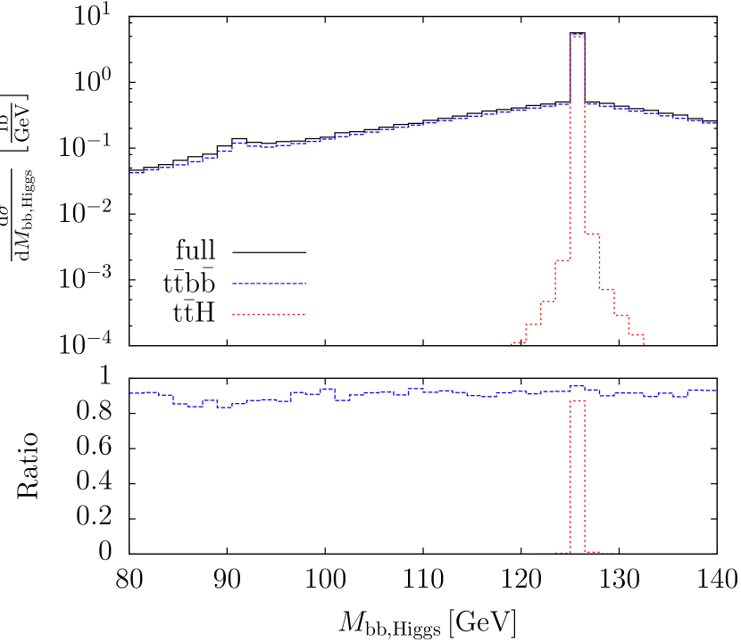
(a)

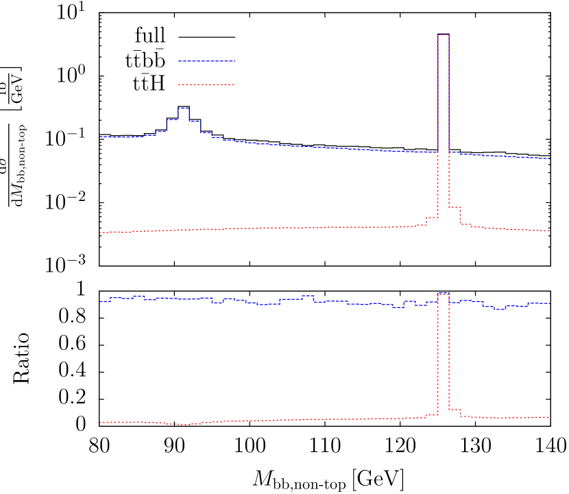
(b)

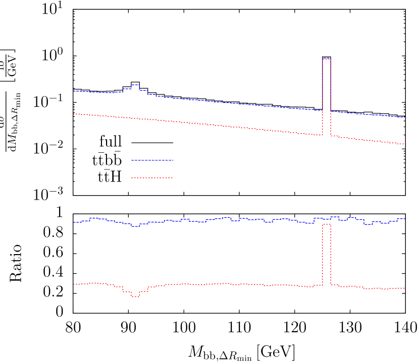
(c)

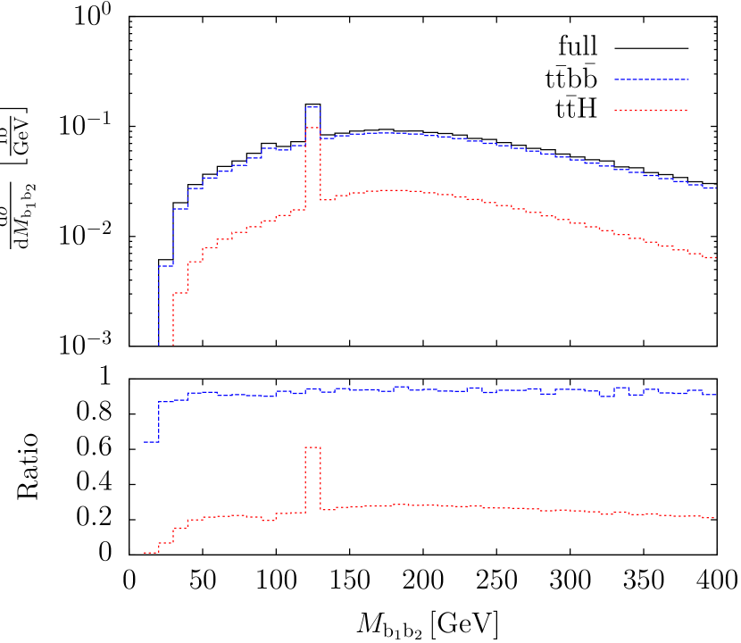
(d)

Figure 2: Invariant-mass distributions at the LHC at $13\,\text{TeV}$ of the b-jet pair that 2(a) forms an invariant mass closest to the Higgs-boson mass (upper left), 2(b) forms an invariant mass determined by top–antitop Breit–Wigner maximum likelihood (upper right), 2(c) forms the smallest distance $\Delta R$ (lower left), 2(d) has the highest transverse momenta (lower right). The lower panels show the relative size of $\text{t}\bar{\text{t}}\text{b}\bar{\text{b}}$ and $\text{t}\bar{\text{t}}\text{H}$ production normalised to the full process.

For this observable we compute the invariant masses of all six b-jet pairs and choose the one that is closest to the Higgs-boson mass used in the Monte Carlo run. Figure 2(a) displays the resulting invariant-mass distribution. For $\text{t}\bar{\text{t}}\text{H}$ production it features a very clear peak at the Higgs-boson mass with a strong drop-off according to the Breit–Wigner shape of the Higgs-boson resonance. Thus, the ratio of $\text{t}\bar{\text{t}}\text{H}$ production and the full process almost vanishes outside the resonant region. The finite off-shell contributions are a result of the pole approximation where the on-shell projected momenta are only applied to the matrix element evaluation, but not to the resonant propagator. The phase-space integration and thus the histogram binning is performed with off-shell momenta. The $\text{t}\bar{\text{t}}\text{b}\bar{\text{b}}$ and the full process have contributions where the Higgs boson is replaced by a Z boson, visible as a bump around the Z-boson mass in the differential distribution.

This observable is strongly biased, since we always choose the b-jet combination that gives the invariant mass closet to the Higgs-boson mass. This explains the rise of the differential cross section for $\text{t}\bar{\text{t}}\text{b}\bar{\text{b}}$ production and the full process towards the Higgs resonance outside the peak.

3.2.2 Invariant mass of b-jet pair determined by top–antitop Breit–Wigner maximum likelihood

Motivated by Ref. ATLAS:2012cpa we determine the two b jets that most likely originate from the decay of the top quark ($\text{t}\to\text{W}^{+}\text{b}\to\ell^{+}\nu_{\ell}\text{b}$) and antitop quark ($\bar{\text{t}}\to\text{W}^{-}\bar{\text{b}}\to\bar{u}d\bar{\text{b}}$, with $u=\text{u},\text{c}$, $d=\text{d},\text{s}$) and plot the invariant mass of the remaining b-jet pair. Since in most events the top quark and antitop quark in $\text{t}\bar{\text{t}}\text{H}$ production are nearly on-shell, the two b jets maximising the corresponding propagator contributions are most likely to originate from the top-quark and antitop-quark decay. To determine the maximising b-jet combination we compute a top-momentum candidate with the charged lepton, neutrino and a b-jet momentum ($p_{\text{b}_{i}}$),

$$p_{\ell^{+}\nu_{\ell}\text{b}_{i}}=p_{\ell^{+}}+p_{\nu_{\ell}}+p_{\text{b}_{i}}$$ (11)

and an analogous antitop-momentum candidate with the two momenta of the non-b jets and a different b-jet momentum ($p_{\text{b}_{j}}$),

$$p_{\text{j}_{1}\text{j}_{2}\text{b}_{j}}=p_{\text{j}_{1}}+p_{\text{j}_{2}}+p_{\text{b}_{j}}.$$ (12)

As b jets originating from the top-quark and antitop-quark decay we select those that maximise the likelihood function $\mathcal{L}$ defined as a product of two Breit–Wigner distributions corresponding to the top-quark and antitop-quark propagators:

$$\mathcal{L}\propto\frac{1}{\Bigl{(}p_{\ell^{+}\nu_{\ell}\text{b}_{i}}^{2}\!-m_{\text{t}}^{2}\Bigr{)}^{2}+\left(m_{\text{t}}\Gamma_{\text{t}}\right)^{2}}\,\frac{1}{\Bigl{(}p_{\text{j}_{1}\text{j}_{2}\text{b}_{j}}^{2}\!-m_{\text{t}}^{2}\Bigr{)}^{2}+\left(m_{\text{t}}\Gamma_{\text{t}}\right)^{2}}.$$ (13)

In Figure 2(b) we present the b-jet-pair invariant mass that has been identified to originate from the Higgs-boson decay by the maximum-likelihood method described above. In the off-shell region the ratio of $\text{t}\bar{\text{t}}\text{H}$ production to the full process drops considerably below the corresponding ratio for the total cross section of about a fourth. Owing to the absence of the bias, the peak in the resonant region is more pronounced for the full process compared the method based on the b-jet-pair invariant mass closest to the Higgs-boson mass (Figure 2(a)), yielding a better signal to background ratio. Since this method tags the b jets resulting from the top and antitop quarks, any resonance in the invariant mass of the remaining b-jet pair is resolved, and thus the Z resonance is clearly visible in the plot.

3.2.3 Invariant mass of minimal $\Delta R$-distance b-jet pair

Next we compute for each event the $\Delta R$ distance of all six b-jet pairs and plot the invariant mass of the pair with the smallest $\Delta R$ distance. Since the Higgs boson, as a scalar particle, decays isotropically, this observable is not sensitive to Higgs-boson production at the $\text{t}\bar{\text{t}}\text{H}$ threshold but potentially for boosted Higgs bosons. Figure 2(c) displays the corresponding invariant-mass distribution for all three scenarios. The Higgs-boson peak is clearly visible in all cases. However, it is less pronounced compared to the Breit–Wigner maximum-likelihood method (Figure 2(b)) and the ratio of peak over background is only weakly enhanced compared to the purely combinatorial effect. Outside the regions of the Higgs and Z-boson resonances the ratio of $\text{t}\bar{\text{t}}\text{H}$ production vs. the full process equals the average value of about a fourth, which we see in the total cross-section ratio. This indicates that the b-jet pair with minimal $\Delta R$ distance is almost evenly distributed among all six possible b-jet pairs, i.e. the method fails to tag the b-jet pair originating from the Higgs-boson decay.

The bump around the Z-boson mass in the differential distributions is weaker as compared to Figure 2(b) and there appears a ditch in the $\text{t}\bar{\text{t}}\text{H}$ ratio because the Z-boson resonance is absent in $\text{t}\bar{\text{t}}\text{H}$ production. The ditch in the $\text{t}\bar{\text{t}}\text{b}\bar{\text{b}}$ ratio is due to relative differences in contributions from resonant Z bosons in the full process and in $\text{t}\bar{\text{t}}\text{b}\bar{\text{b}}$ production. Thus, in the considered set-up this method is not suitable to tag the Higgs boson. This might be different if strongly boosted Higgs bosons are required.

3.2.4 Invariant mass of two hardest b jets

For comparison we show the distribution in the invariant mass of the pair of the two hardest b jets in Figure 2(d). Also here the Higgs-boson signal is clearly visible for all processes but there is no enhancement above the purely statistical level. The apparently smaller enhancement of the Higgs peak as compared to Figure 2(c) is basically due to the larger bin width ($10\,\text{GeV}$ as compared to $1.5\,\text{GeV}$). Furthermore, outside the resonance regions $\text{t}\bar{\text{t}}\text{H}$ production is about a fourth of the full process, as for the total cross section.

3.2.5 Further differential distributions

In this section we investigate further differential distributions concentrating on observables that show deviations in the shape between the full process and the approximations. Some other distributions which show no significant shape deviations are listed in Appendix B.

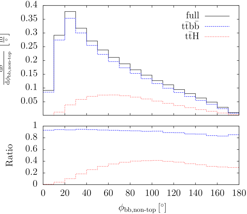
(a)

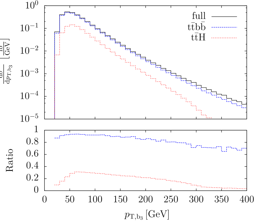
(b)

(c)

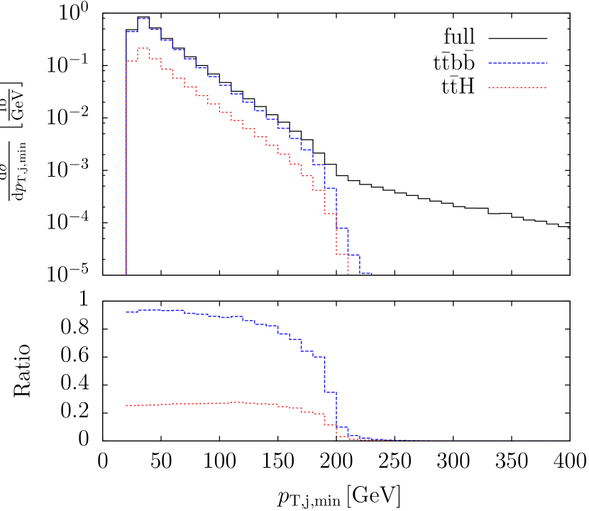
(d)

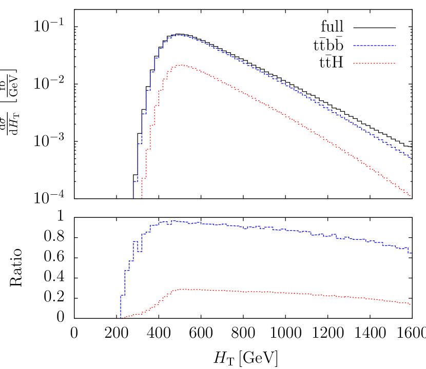
(e)

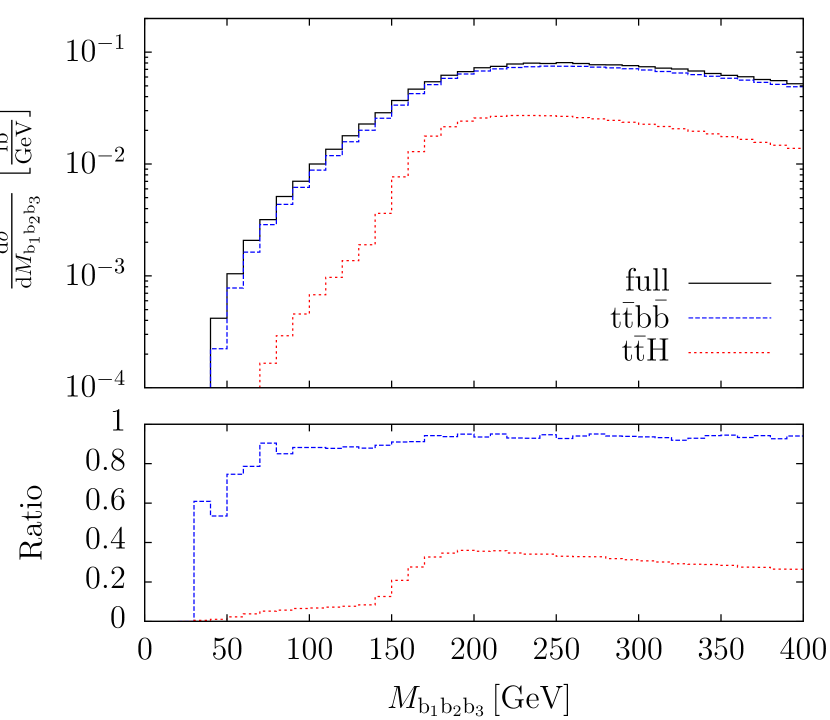
(f)

Figure 3: Differential distributions at the LHC at $13\,\text{TeV}$ exhibiting shape deviations between the full process and $\text{t}\bar{\text{t}}\text{b}\bar{\text{b}}$ or $\text{t}\bar{\text{t}}\text{H}$ production: 3(a) azimuthal separation of the b-jet pair determined by top–antitop Breit–Wigner maximum likelihood (upper left), 3(b) transverse momentum of the 3rd-hardest b jet (upper right), 3(c) transverse momentum of the hardest non-b jet (middle left), 3(d) transverse momentum of the softest non-b jet (middle right), 3(e) total transverse energy (lower left), 3(f) invariant mass of the three hardest b jets (lower right). The lower panels show the relative size of $\text{t}\bar{\text{t}}\text{b}\bar{\text{b}}$ and $\text{t}\bar{\text{t}}\text{H}$ production normalised to the full process.

Figure 3(a) shows the azimuthal separation of the b-jet pair determined by top–antitop Breit–Wigner maximum likelihood according to Section 3.2.2. While $\text{t}\bar{\text{t}}\text{b}\bar{\text{b}}$ production and the full process yield a very similar shape, $\text{t}\bar{\text{t}}\text{H}$ production exhibits clearly a different shape. This behaviour can be explained by the dominant production mechanisms of bottom–antibottom pairs. In the signal process these result from the Higgs boson and owing to the finite Higgs-boson mass tend to have a finite opening angle. In the background processes the bottom–antibottom pairs result mainly from gluons and thus tend to be collinear leading to a peak at small $\phi_{\text{b}\text{b}}$ that is cut off by the acceptance function. Thus, this distribution can help to separate bottom–antibottom pairs resulting from Higgs bosons from those of other origin.

Figure 3(b) displays the transverse-momentum distribution of the third-hardest b jet. We find that all three approximations are similar in shape for $p_{\text{T}}$ values below $150\,\text{GeV}$. For higher transverse momenta the distribution for $\text{t}\bar{\text{t}}\text{H}$ production diverges from those of the full process and $\text{t}\bar{\text{t}}\text{b}\bar{\text{b}}$ production. We do not see this behaviour in the transverse momentum distributions of the two harder b jets (see Figure 5(c) in Appendix B) but to some extent in the one of the fourth-hardest b jet. This results from the fact that in the $\text{t}\bar{\text{t}}\text{H}$ signal all b jets originate from heavy-particle decays, while in the full process some are directly produced yielding more b jets with high transverse momenta.

The distributions in the transverse momenta of the two non-b jets are displayed in Figures 3(c)–3(d). For the hardest non-b jet, we find a similar picture as for the 3rd hardest b jet and an enhancement for the full process relative to $\text{t}\bar{\text{t}}\text{b}\bar{\text{b}}$ production and $\text{t}\bar{\text{t}}\text{H}$ production for transverse momenta above $150\,\text{GeV}$. The explanation is similar as in the preceding case. While in the $\text{t}\bar{\text{t}}\text{b}\bar{\text{b}}$ process the jets originate from the top-quark decay, in the full process they can be produced directly leading to more jet activity at high transverse momenta. In the case of the second hardest jet both approximations exhibit a strong drop near $p_{\rm T,j,min}=200\,\text{GeV}$. For higher transverse momenta two jets originating from W-boson decay are too collinear to pass the rapidity–azimuthal-angle-separation cut of $\Delta R_{\text{j}\text{j}}>0.4$ such that the corresponding events are eliminated. On the other hand, events with jets pairs with higher invariant masses, which are present in the full process, are not cut.

The sum of all transverse energies (including missing transverse energy) is depicted in Figure 3(e). For small $H_{\rm T}$ the different thresholds of the approximations are clearly visible. For $H_{\rm T}\sim 400\,\text{GeV}$–$800\,\text{GeV}$ the $\text{t}\bar{\text{t}}\text{b}\bar{\text{b}}$ approximation describes the full process within $10\,\%$. As it decreases stronger with increasing $H_{\rm T}$ the deviation becomes larger above $800\,\text{GeV}$. Since $H_{\rm T}$ incorporates all transverse energies of the process it is a measure for the average deviation of the transverse energies between the approximations and the full process.

Finally, Figure 3(f) presents the invariant mass of the three hardest b jets. Below the threshold $M_{\text{H}}+p_{\mathrm{T},\text{b},\mathrm{cut}}\approx 150\,\text{GeV}$ the signal process is strongly suppressed, above its ratio to the full process rises to $36\,\%$ at $M_{\mathrm{b_{1}b_{2}b_{3}}}\sim 195\,\text{GeV}$ and then drops slowly to $26\,\%$ at $M_{\mathrm{b_{1}b_{2}b_{3}}}\sim 400\,\text{GeV}$. The ratio of $\text{t}\bar{\text{t}}\text{b}\bar{\text{b}}$ production and the full process on the other hand is roughly constant for $M_{\mathrm{b_{1}b_{2}b_{3}}}\;\raisebox{-3.00003pt}{$\stackrel{{\scriptstyle\displaystyle>}}{{\sim}}$}\;70\,\text{GeV}$.

3.3 Interference effects in differential distributions

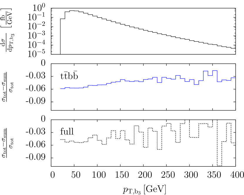
(a)

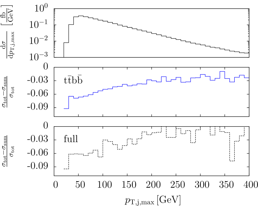
(b)

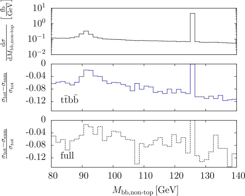
(c)

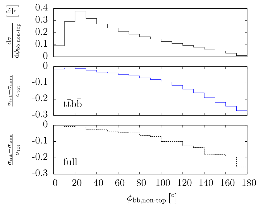
(d)

Figure 4: Interference effects versus 4(a) transverse momentum of the 3rd-hardest b jet (upper left), 4(b) transverse momentum of the hardest non-b jet (upper right), 4(c) invariant mass of the of the b-jet pair determined by top–antitop Breit–Wigner maximum likelihood (lower left), 4(d) azimuthal separation of the b-jet pair determined by top–antitop Breit–Wigner maximum likelihood (lower right). The lower panels show the relative interference effects of $\text{t}\bar{\text{t}}\text{b}\bar{\text{b}}$ production and the full process, respectively. The upper panel shows the corresponding differential distribution of the full process as reference.

In this section we study in detail the effects of the interference contributions between matrix elements of different orders in $\alpha_{\text{s}}$. For most distributions we find a uniform shift by roughly the same amount as for the total cross section, i.e. about $5\,\%$ for $\text{t}\bar{\text{t}}\text{b}\bar{\text{b}}$ production and the full process (interference effects are absent in $\text{t}\bar{\text{t}}\text{H}$ production). For both scenarios we observe a few kinematical distributions that are sensitive to these interference effects. The upper panels of Figure 4 show the results for the full process and the central and lower panels highlight the interference effects. Specifically, the central panels show the relative difference ${(\sigma_{\text{tot}}-\sigma_{\text{sum}})}/{\sigma_{\text{tot}}}$ for $\text{t}\bar{\text{t}}\text{b}\bar{\text{b}}$ production with a solid blue line and the lower panels the same relative difference for the full process with a dashed line.

In Figures 4(a) and 4(b) we see that the effect of the interference for the distributions in the transverse momentum of the third-hardest b jet and for the harder non-b jet, respectively, varies monotonically with increasing $p_{\text{T}}$ from $-6\,\%$ to $-2\,\%$. Figure 4(c) shows the interference effects on the distribution of the invariant mass of the b-jet pair determined by top–antitop Breit–Wigner maximum likelihood. The suppression of interference in the regions of the Higgs- and Z-boson resonances is clearly visible. For invariant masses above the Higgs threshold the interference effect exceeds $-10\,\%$. As shown in Figure 4(d), the relative interference effects grow with increasing azimuthal-angle separation of the b-jet pair determined by top–antitop Breit–Wigner maximum likelihood from almost zero at small angles to $-25\,\%$ for $\phi_{\mathrm{bb,non\textnormal{-}top}}=180^{\circ}$, while the cross section drops with increasing azimuthal-angle separation. Also in the distributions the dominant interference effects arise from diagrams of order $\mathcal{O}{\left(\alpha_{\text{s}}\alpha^{3}\right)}$ involving $t$-channel W-boson exchange interfering with diagrams of order $\mathcal{O}{\left(\alpha_{\text{s}}^{2}\alpha^{2}\right)}$. Interferences with diagrams for $\text{t}\bar{\text{t}}\text{H}$ production are by a factor five or more smaller.

4 Conclusion and outlook

We have presented an analysis of the irreducible background for $\text{t}\bar{\text{t}}\text{H}$ production at the LHC. Specifically, we have compared the full Standard Model cross section for the production of four b jets, two jets, one identified charged lepton and missing energy with the contributions from the subprocesses $\text{t}\bar{\text{t}}\text{b}\bar{\text{b}}$ production and $\text{t}\bar{\text{t}}\text{H}$ production, obtained using the pole approximation. With standard acceptance cuts we find that the total cross section of $\text{t}\bar{\text{t}}\text{H}$ production and decay is roughly a fourth of the full process, while $\text{t}\bar{\text{t}}\text{b}\bar{\text{b}}$ production constitutes the major contribution to the full process with about $92\,\%$. For all scenarios the bulk of the cross section originates from gluon-induced processes.

We analysed various b-jet-pair invariant-mass distributions based on different methods to select two of the four b jets to be identified with the decay products of the Higgs boson. We find that assigning two b jets to the top- and antitop-quark decay by maximising a combined Breit–Wigner likelihood function and assigning the remaining two b jets to the potential Higgs boson yields a good unbiased determination of the b-jet pair originating from the Higgs-boson decay.

We investigated the interferences between contributions to the matrix element of different orders in the strong and electroweak couplings constants. We find that interference effects are only sizeable for gluon-induced processes and lower the hadronic cross section by about $5\,\%$. The dominant contributions result from interferences of the QCD $\text{t}\bar{\text{t}}\text{b}\bar{\text{b}}$ production diagrams of order $\mathcal{O}{\left(\alpha_{\text{s}}^{2}\alpha^{2}\right)}$ with diagrams of order $\mathcal{O}{\left(\alpha_{\text{s}}\alpha^{3}\right)}$ involving t-channel W-boson exchange. Interferences between the dominant background and the $\text{t}\bar{\text{t}}\text{H}$ signal on the other hand are below one per cent. In most of the differential distributions the interference effects lead to a constant shift. We found, however, a few distributions where non-uniform shape changes appear.

Our analysis demonstrates the complexity of this process and provides useful information for a future NLO calculation. We found that the $\text{t}\bar{\text{t}}\text{b}\bar{\text{b}}$ process provides a good approximation to the full process, with a deviation of only about $8\,\%$ for the total cross section and a uniform shift for most differential distributions. While the QCD corrections to the leading QCD contributions to $\text{t}\bar{\text{t}}\text{b}\bar{\text{b}}$ production are already known, a calculation of the NLO corrections to the full $\text{t}\bar{\text{t}}\text{b}\bar{\text{b}}$ process should be feasible with available tools Actis:2012qn ; Denner:2014gla .

Appendix A On-shell projection

In this appendix we discuss some details of our implementation of the pole approximation. For $\text{t}\bar{\text{t}}\text{b}\bar{\text{b}}$ production ($\text{t}\bar{\text{t}}\text{H}$ production) we compute the matrix element with on-shell momenta for the top quarks (and the Higgs boson) and consider off-shell effects only in the corresponding propagators of the unstable particles. Thus, starting from off-shell momenta we use an on-shell projection to generate the momenta of the resonant particles. Since the procedure of on-shell projection is not uniquely defined we impose suitable requirements. The matrix element is strongly sensible to resonances and hence we project such as to retain sensible invariants as far as possible. As a consequence of the on-shell projection of the top quarks we also need to incorporate proper on-shell projections for their decay products.

A.1 Higgs-boson on-shell projection

For $\text{t}\bar{\text{t}}\text{H}$ production we project the Higgs boson in $\text{H}\to\text{b}\bar{\text{b}}$ on-shell, such that $\hat{p}_{\text{H}}^{2}=m_{\text{H}}^{2}$, $\hat{p}_{\text{b}}^{2}=p_{\text{b}}^{2}=m_{\text{b}}^{2}$, $\hat{p}_{\bar{\text{b}}}^{2}=p_{\bar{\text{b}}}^{2}=m_{\text{b}}^{2}$ and $\hat{p}_{\text{H}}=\hat{p}_{\text{b}}+\hat{p}_{\bar{\text{b}}}$, where $\hat{p}$ denotes the projected momentum corresponding to $p$. With these constraints the projected momenta are obtained as

$$\hat{p}_{\text{b}} =\alpha\,\frac{p_{\text{b}}-p_{\bar{\text{b}}}}{2}+\beta\,\frac{p_{\text{b}}+p_{\bar{\text{b}}}}{2},$$ (14)

$$\hat{p}_{\bar{\text{b}}} =\alpha\,\frac{p_{\bar{\text{b}}}-p_{\text{b}}}{2}+\beta\,\frac{p_{\text{b}}+p_{\bar{\text{b}}}}{2},$$

$$\hat{p}_{\text{H}} =\beta p_{\text{H}},$$

where

$$\alpha=\sqrt{\frac{M_{\text{H}}^{2}-4m_{\text{b}}^{2}}{p_{\text{H}}^{2}-4m_{\text{b}}^{2}}},\qquad\beta=\frac{M_{\text{H}}}{\sqrt{p_{\text{H}}^{2}}}.$$ (15)

We choose the positive solution for $\alpha$ to minimise momenta alteration.

To preserve momentum conservation we choose to adjust the top-quark momentum according to

$$p_{\text{t}}^{\prime}=p_{\text{t}}+p_{\text{H}}-\hat{p}_{\text{H}}.$$ (16)

Adjusting instead the antitop-quark momentum accordingly would lead to a slightly different but equally well performing on-shell projection.

A.2 Top- and antitop-quark on-shell projection

We project the top and the antitop quarks on-shell simultaneously. In the case of the $\text{t}\bar{\text{t}}\text{H}$ approximation the Higgs boson has been projected on-shell (see above) and the top-quark momentum gets adjusted (16) to preserve momentum conservation. In the following we use the adjusted top-quark momentum $p_{\text{t}}^{\prime}$ for $\text{t}\bar{\text{t}}\text{H}$ production while for $\text{t}\bar{\text{t}}\text{b}\bar{\text{b}}$ production the original momentum is used. The antitop-quark momentum is the original one $p_{\bar{\text{t}}}$ for both the $\text{t}\bar{\text{t}}\text{H}$ and the $\text{t}\bar{\text{t}}\text{b}\bar{\text{b}}$ scenario.

The imposed requirements for the simultaneous top and antitop projection are the on-shell conditions $\hat{p}_{\text{t}}^{2}=m_{\text{t}}^{2}$ and $\hat{p}_{\bar{\text{t}}}^{2}=m_{\text{t}}^{2}$ and momentum conservation, $\hat{p}_{\text{t}}+\hat{p}_{\bar{\text{t}}}=p_{\text{t}}^{\prime}+p_{\bar{\text{t}}}$. We consider the general case of two momenta $p_{1}$ and $p_{2}$ to be suitably projected. We define $q=p_{1}+p_{2}$ and seek to construct projected momenta $\hat{p}_{1}$ and $\hat{p}_{2}$ fulfilling $\hat{p}_{1}+\hat{p}_{2}=q$ and $\hat{p}_{1}^{2}$ and $\hat{p}_{2}^{2}$ fixed by given values not necessarily the on-shell conditions $\hat{p}_{1}^{2}=m_{1}^{2}$ and $\hat{p}_{2}^{2}=m_{2}^{2}$. With the ansatz

$$\hat{p}_{1}=\xi p_{1}+\eta p_{2},\qquad\hat{p}_{2}=(1-\xi)p_{1}+(1-\eta)p_{2}$$ (17)

we obtain

$$\xi=\frac{\left(\left(p_{1}+p_{2}\right)^{2}+\hat{p}_{1}^{2}-\hat{p}_{2}^{2}\right)-2\eta\left(p_{2}^{2}+p_{1}p_{2}\right)}{2\left(p_{1}^{2}+p_{1}p_{2}\right)}$$ (18)

and the quadratic equation for the determination of $\eta$:

$$0= \eta^{2}\left[p_{1}^{2}p_{2}-p_{2}^{2}p_{1}+(p_{1}p_{2})(p_{2}-p_{1})\right]^{2}$$ (19)

$$+\eta\left[\left(p_{1}+p_{2}\right)^{2}+\hat{p}_{1}^{2}-\hat{p}_{2}^{2}\right]\left[(p_{1}p_{2})^{2}-p_{1}^{2}p_{2}^{2}\right]$$

$$+\frac{1}{4}\left[\left(p_{1}+p_{2}\right)^{2}+\hat{p}_{1}^{2}-\hat{p}_{2}^{2}\right]^{2}p_{1}^{2}-\left(p_{1}^{2}+p_{1}p_{2}\right)^{2}\hat{p}_{1}^{2}.$$

We choose the smaller solution for $\eta$ to minimise momenta alteration. For the on-shell projection of the top quark and antitop quark we identify $p_{1}\to p_{\bar{\text{t}}}$, $p_{2}\to p_{\text{t}}^{\prime}$, analogously for the projected momenta, and $\hat{p}_{1}^{2}=\hat{p}_{2}^{2}=m_{\text{t}}^{2}$ .

A.3 On-shell projection of the top- and antitop-quark decay products

The on-shell projection of the top and antitop quark alters the momenta of their decay products, which have to be adjusted accordingly. We compute new momenta of the bottom ($p_{\text{b}_{\text{t}}}^{\prime}$) from the top-quark decay ($\text{t}\to\text{W}^{+}\text{b}$) and antibottom ($p_{\bar{\text{b}}_{\bar{\text{t}}}}^{\prime}$) from the antitop-quark decay ($\bar{\text{t}}\to\text{W}^{-}\bar{\text{b}}$), respectively, via

$$p_{\text{b}_{\text{t}}}^{\prime}=\hat{p}_{\text{t}}-p_{\text{W}^{+}},\qquad p_{\bar{\text{b}}_{\bar{\text{t}}}}^{\prime}=\hat{p}_{\bar{\text{t}}}-p_{\text{W}^{-}}$$ (20)

and project them on-shell. To this end we project the $\text{W}^{+}$ and b simultaneously with the requirements $\hat{p}_{\text{W}^{+}}+\hat{p}_{\text{b}_{\text{t}}}=p_{\text{W}^{+}}+p_{\text{b}_{\text{t}}}^{\prime}$, $\hat{p}_{\text{b}_{\text{t}}}^{2}=m_{\text{b}}^{2}$ and $\hat{p}_{\text{W}^{+}}^{2}=p_{\text{W}^{+}}^{2}$. The latter condition preserves the resonance of the $\text{W}^{+}$ propagator, since the $\text{W}^{+}$ is likely to be nearly on-shell and an alteration of its propagator is undesirable. We use a similar projection as in Section A.2, i.e.

$$\hat{p}_{\text{W}^{+}} =\tilde{\xi}p_{\text{W}^{+}}+\tilde{\eta}p_{\text{b}_{\text{t}}}^{\prime},$$ (21)

$$\hat{p}_{\text{b}_{\text{t}}} =(1-\tilde{\xi})p_{\text{W}^{+}}+(1-\tilde{\eta})p_{\text{b}_{\text{t}}}^{\prime}$$

with (18) and (19) and the identification $p_{1}\to p_{\text{W}^{+}}$, $\hat{p}_{1}^{2}\to p_{\text{W}^{+}}^{2}$, $p_{2}\to p_{\text{b}_{\text{t}}}^{\prime}$, and $\hat{p}_{2}^{2}\to m_{\text{b}}^{2}$. Analogously we project $\text{W}^{-}$ and $\bar{\text{b}}$ of the decay $\bar{\text{t}}\to\text{W}^{-}\bar{\text{b}}$.

Two more projections are required for the decays $\text{W}^{+}\to\ell^{+}\nu_{\ell}$ and $\text{W}^{-}\to\bar{\text{u}}\text{d}$ (or $\text{W}^{-}\to\bar{\text{c}}\text{s}$) to ensure the on-shellness of the final-state particles. We explain the procedure by the projection of the charged lepton and neutrino. We first redefine the neutrino momentum via

$$p^{\prime}_{\nu_{\ell}}=\hat{p}_{\text{W}^{+}}-p_{\ell^{+}}$$ (22)

to restore momentum conservation. Then, we make the ansatz

$$\hat{p}_{\ell^{+}}=\alpha p_{\ell^{+}},\qquad\hat{p}_{\nu_{\ell}}=\hat{p}_{\text{W}^{+}}-\hat{p}_{\ell^{+}}$$ (23)

that trivially fulfils the on-shell condition for the charged lepton, $\hat{p}_{\ell^{+}}^{2}=0$. Requiring the projected neutrino momentum to be on-shell yields the following on-shell projected momenta of the $\text{W}^{+}$ decay products in $\text{W}^{+}\to\ell^{+}\nu_{\ell}$:

$$\hat{p}_{\nu_{\ell}}=p^{\prime}_{\nu_{\ell}}-\frac{p_{\nu_{\ell}}^{\prime 2}}{2p^{\prime}_{\nu_{\ell}}p_{\ell^{+}}}p_{\ell^{+}},\qquad\hat{p}_{\ell^{+}}=\left(1+\frac{p_{\nu_{\ell}}^{\prime 2}}{2p^{\prime}_{\nu_{\ell}}p_{\ell^{+}}}\right)p_{\ell^{+}}.$$ (24)

Analogously we obtain for the projection of the $\text{W}^{-}$ decay products in $\text{W}^{-}\to\bar{\text{u}}\text{d}(\bar{\text{c}}\text{s})$:

$$\hat{p}_{\text{d}(\text{s})}=p^{\prime}_{\text{d}(\text{s})}-\frac{p_{\text{d}(\text{s})}^{\prime 2}}{2p^{\prime}_{\text{d}(\text{s})}p_{\bar{\text{u}}(\bar{\text{c}})}}p_{\bar{\text{u}}(\bar{\text{c}})},\qquad\hat{p}_{\bar{\text{u}}(\bar{\text{c}})}=\left(1+\frac{p_{\text{d}(\text{s})}^{\prime 2}}{2p^{\prime}_{\text{d}(\text{s})}p_{\bar{\text{u}}(\bar{\text{c}})}}\right)p_{\bar{\text{u}}(\bar{\text{c}})}$$ (25)

with

$$\hat{p}^{\prime}_{\text{d}(\text{s})}=\hat{p}_{\text{W}^{-}}-\hat{p}_{\bar{\text{u}}(\bar{\text{c}})}.$$ (26)

Thus, we perform six projections in total for $\text{t}\bar{\text{t}}\text{H}$ production and five for $\text{t}\bar{\text{t}}\text{b}\bar{\text{b}}$ production. Of course, the on-shell projections do not change the momenta, if the resonant particles are already on shell.

Appendix B Further differential distributions

In this appendix we present further differential distributions which exhibit only minor shape deviations between the full process and the approximations. As for the total cross section we find for most distributions a constant offset of $8\,\%$ between the full process and the $\text{t}\bar{\text{t}}\text{b}\bar{\text{b}}$ approximation and about a factor four between the full process and the $\text{t}\bar{\text{t}}\text{H}$ approximation. Only in tails of distributions larger deviations between the full process and the approximations appear.

In Figures 5(a)–5(b) we show the transverse momentum and the rapidity distribution of the identified charged lepton, while the transverse momentum and the rapidity distribution of the hardest b jet are depicted in Figures 5(c)–5(d). Finally, the missing transverse momentum and the transverse mass of the charged lepton, the neutrino and the hardest b jet are provided in Figures 5(e)–5(f).

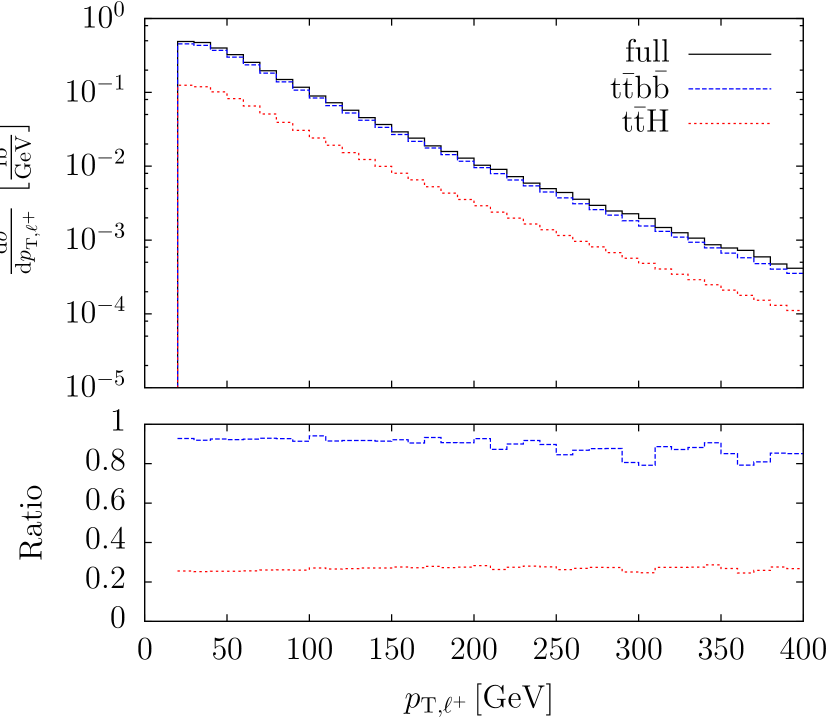
(a)

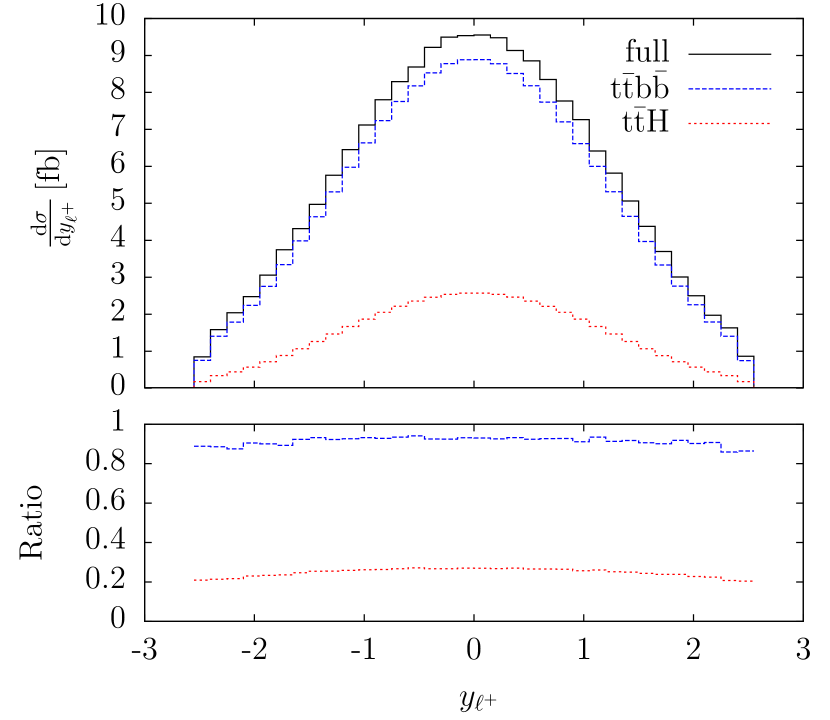
(b)

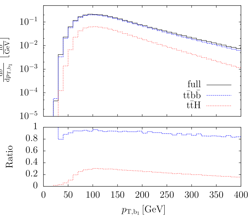
(c)

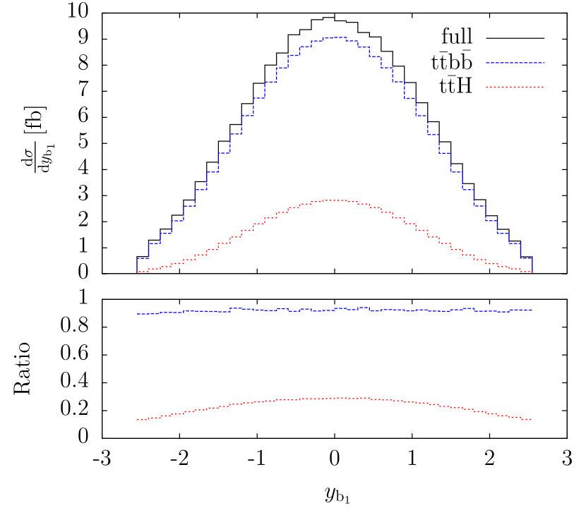
(d)

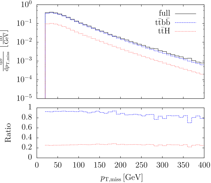
(e)

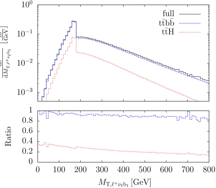
(f)

Figure 5: Standard differential distributions at the LHC at $13\,\text{TeV}$ for the full process, $\text{t}\bar{\text{t}}\text{b}\bar{\text{b}}$ production and $\text{t}\bar{\text{t}}\text{H}$ production: 5(a) transverse momentum of the charged lepton (upper left), 5(b) rapidity of the charged lepton (upper right), 5(c) transverse momentum of the hardest b jet (middle left), 5(d) rapidity of the hardest b jet (middle right), 5(e) missing transverse momentum (lower left), 5(f) transverse mass of the $\ell^{+}\nu_{\ell}\text{b}_{1}$ system (lower right right). The lower panels show the relative size of $\text{t}\bar{\text{t}}\text{b}\bar{\text{b}}$ and $\text{t}\bar{\text{t}}\text{H}$ production normalised to the full process.

References

- (1) ATLAS Collaboration, G. Aad et al., Observation of a new particle in the search for the Standard Model Higgs boson with the ATLAS detector at the LHC, Phys.Lett. B716 (2012) 1–29, [arXiv:1207.7214].
- (2) CMS Collaboration, S. Chatrchyan et al., Observation of a new boson at a mass of 125 GeV with the CMS experiment at the LHC, Phys.Lett. B716 (2012) 30–61, [arXiv:1207.7235].
- (3) ATLAS Collaboration, Search for the Standard Model Higgs boson produced in association with top quarks in proton-proton collisions at TeV using the ATLAS detector, ATLAS-CONF-2012-135, ATLAS-COM-CONF-2012-162.
- (4) ATLAS Collaboration, Search for the Standard Model Higgs boson produced in association with top quarks and decaying to in pp collisions at 8 TeV with the ATLAS detector at the LHC, ATLAS-CONF-2014-011, ATLAS-COM-CONF-2014-004.
- (5) ATLAS Collaboration, G. Aad et al., Search for produced in association with top quarks and constraints on the Yukawa coupling between the top quark and the Higgs boson using data taken at 7 TeV and 8 TeV with the ATLAS detector, arXiv:1409.3122.
- (6) CMS Collaboration, Search for Higgs boson production in association with top quark pairs in pp collisions, CMS-PAS-HIG-12-025.
- (7) CMS Collaboration, Search for Higgs Boson Production in Association with a Top-Quark Pair and Decaying to Bottom Quarks or Tau Leptons, CMS-PAS-HIG-13-019.
- (8) CMS Collaboration, Search for ttH production in events where H decays to photons at 8 TeV collisions, Tech. Rep. CMS-PAS-HIG-13-015, CERN, Geneva, 2013.
- (9) CMS Collaboration, S. Chatrchyan et al., Search for the standard model Higgs boson produced in association with a top-quark pair in pp collisions at the LHC, JHEP 1305 (2013) 145, [arXiv:1303.0763].
- (10) CMS Collaboration, V. Khachatryan et al., Search for the associated production of the Higgs boson with a top-quark pair, JHEP 1409 (2014) 087, [arXiv:1408.1682].
- (11) R. Raitio and W. W. Wada, Higgs Boson Production at Large Transverse Momentum in QCD, Phys.Rev. D19 (1979) 941.
- (12) J. N. Ng and P. Zakarauskas, A QCD Parton Calculation of Conjoined Production of Higgs Bosons and Heavy Flavors in Collision, Phys.Rev. D29 (1984) 876.
- (13) Z. Kunszt, Associated Production of Heavy Higgs Boson with Top Quarks, Nucl.Phys. B247 (1984) 339.
- (14) J. Gunion, Associated top anti-top Higgs production as a large source of W H events: Implications for Higgs detection in the final state, Phys.Lett. B261 (1991) 510–517.
- (15) W. J. Marciano and F. E. Paige, Associated production of Higgs bosons with pairs, Phys.Rev.Lett. 66 (1991) 2433–2435.
- (16) W. Beenakker, S. Dittmaier, M. Krämer, B. Plümper, M. Spira, et al., Higgs radiation off top quarks at the Tevatron and the LHC, Phys.Rev.Lett. 87 (2001) 201805, [hep-ph/0107081].
- (17) W. Beenakker, S. Dittmaier, M. Krämer, B. Plümper, M. Spira, et al., NLO QCD corrections to production in hadron collisions, Nucl.Phys. B653 (2003) 151–203, [hep-ph/0211352].
- (18) L. Reina and S. Dawson, Next-to-leading order results for production at the Tevatron, Phys.Rev.Lett. 87 (2001) 201804, [hep-ph/0107101].
- (19) S. Dawson, L. Orr, L. Reina, and D. Wackeroth, Associated top quark Higgs boson production at the LHC, Phys.Rev. D67 (2003) 071503, [hep-ph/0211438].
- (20) S. Dawson, C. Jackson, L. Orr, L. Reina, and D. Wackeroth, Associated Higgs production with top quarks at the large hadron collider: NLO QCD corrections, Phys.Rev. D68 (2003) 034022, [hep-ph/0305087].
- (21) R. Frederix, S. Frixione, V. Hirschi, F. Maltoni, R. Pittau, et al., Scalar and pseudoscalar Higgs production in association with a top-antitop pair, Phys.Lett. B701 (2011) 427–433, [arXiv:1104.5613].
- (22) M. Garzelli, A. Kardos, C. Papadopoulos, and Z. Trócsányi, Standard Model Higgs boson production in association with a top anti-top pair at NLO with parton showering, Europhys.Lett. 96 (2011) 11001, [arXiv:1108.0387].
- (23) S. Frixione, V. Hirschi, D. Pagani, H. S. Shao, and M. Zaro, Weak corrections to Higgs hadroproduction in association with a top-quark pair, arXiv:1407.0823.
- (24) Z. Yu, M. Wen-Gan, Z. Ren-You, C. Chong, and G. Lei, QCD NLO and EW NLO corrections to production with top quark decays at hadron collider, arXiv:1407.1110.
- (25) A. Bredenstein, A. Denner, S. Dittmaier, and S. Pozzorini, NLO QCD corrections to production at the LHC: 1. Quark-antiquark annihilation, JHEP 0808 (2008) 108, [arXiv:0807.1248].
- (26) A. Bredenstein, A. Denner, S. Dittmaier, and S. Pozzorini, NLO QCD corrections to at the LHC, Phys.Rev.Lett. 103 (2009) 012002, [arXiv:0905.0110].
- (27) G. Bevilacqua, M. Czakon, C. Papadopoulos, R. Pittau, and M. Worek, Assault on the NLO Wishlist: , JHEP 0909 (2009) 109, [arXiv:0907.4723].
- (28) A. Bredenstein, A. Denner, S. Dittmaier, and S. Pozzorini, NLO QCD Corrections to Top Anti-Top Bottom Anti-Bottom Production at the LHC: 2. full hadronic results, JHEP 1003 (2010) 021, [arXiv:1001.4006].
- (29) A. Kardos and Z. Trócsányi, Hadroproduction of t anti-t pair with a b anti-b pair using PowHel, J.Phys. G41 (2014) 075005, [arXiv:1303.6291].
- (30) F. Cascioli, P. Maierhöfer, N. Moretti, S. Pozzorini, and F. Siegert, NLO matching for production with massive b-quarks, arXiv:1309.5912.
- (31) M. V. Garzelli, A. Kardos, and Z. Trócsányi, hadroproduction at NLO accuracy matched with parton shower, PoS EPS-HEP2013 (2013) 253.
- (32) SM and NLO Multileg Working Group, J. Andersen et al., The SM and NLO Multileg Working Group: Summary report, arXiv:1003.1241.
- (33) LHC Higgs Cross Section Working Group, S. Dittmaier et al., Handbook of LHC Higgs Cross Sections: 1. Inclusive Observables, arXiv:1101.0593.
- (34) LHC Higgs Cross Section Working Group, S. Dittmaier et al., Handbook of LHC Higgs Cross Sections: 2. Differential Distributions, arXiv:1201.3084.
- (35) LHC Higgs Cross Section Working Group, S. Heinemeyer et al., Handbook of LHC Higgs Cross Sections: 3. Higgs Properties, arXiv:1307.1347.
- (36) K. Melnikov, M. Schulze, and A. Scharf, QCD corrections to top quark pair production in association with a photon at hadron colliders, Phys.Rev. D83 (2011) 074013, [arXiv:1102.1967].
- (37) K. Melnikov, A. Scharf, and M. Schulze, Top quark pair production in association with a jet: QCD corrections and jet radiation in top quark decays, Phys.Rev. D85 (2012) 054002, [arXiv:1111.4991].
- (38) S. Actis, A. Denner, L. Hofer, A. Scharf, and S. Uccirati, Recursive generation of one-loop amplitudes in the Standard Model, JHEP 1304 (2013) 037, [arXiv:1211.6316].
- (39) A. Denner, S. Dittmaier, M. Roth, and D. Wackeroth, Predictions for all processes fermions , Nucl.Phys. B560 (1999) 33–65, [hep-ph/9904472].
- (40) A. Denner, S. Dittmaier, M. Roth, and L. Wieders, Electroweak corrections to charged-current fermion processes: Technical details and further results, Nucl.Phys. B724 (2005) 247–294, [hep-ph/0505042].
- (41) A. Denner and S. Dittmaier, The Complex-mass scheme for perturbative calculations with unstable particles, Nucl.Phys.Proc.Suppl. 160 (2006) 22–26, [hep-ph/0605312].
- (42) D. Y. Bardin, A. Leike, T. Riemann, and M. Sachwitz, Energy Dependent Width Effects in Annihilation Near the Z Boson Pole, Phys.Lett. B206 (1988) 539–542.
- (43) M. Jezabek and J. H. Kühn, QCD corrections to semileptonic decays of heavy quarks, Nucl.Phys. B314 (1989) 1.
- (44) A. Denner, S. Dittmaier, M. Roth, and D. Wackeroth, Electroweak radiative corrections to 4 fermions in double pole approximation: The RACOONWW approach, Nucl.Phys. B587 (2000) 67–117, [hep-ph/0006307].
- (45) A. Denner, S. Dittmaier, and L. Hofer, COLLIER – A fortran-library for one-loop integrals, PoS LL2014 (2014) 071, [arXiv:1407.0087].