ON GENERATING SETS OF YOSHIKAWA MOVES FOR MARKED GRAPH DIAGRAMS OF SURFACE-LINKS

Abstract

A marked graph diagram is a link diagram possibly with marked $4$-valent vertices. S. J. Lomonaco, Jr. and K. Yoshikawa introduced a method of representing surface-links by marked graph diagrams. Specially, K. Yoshikawa suggested local moves on marked graph diagrams, nowadays called Yoshikawa moves. It is now known that two marked graph diagrams representing equivalent surface-links are related by a finite sequence of these Yoshikawa moves. In this paper, we provide some generating sets of Yoshikawa moves on marked graph diagrams representing unoriented surface-links, and also oriented surface-links. We also discuss independence of certain Yoshikawa moves from the other moves.

Mathematics Subject Classification 2000: 57Q45; 57M25.

Key words and phrases: ch-diagram; generating set; marked graph diagram; surface-link; Yoshikawa moves; independence of Yoshikawa moves.

1 Introduction

By a surface-link we mean a closed 2-manifold smoothly (or piecewise linearly and locally flatly) embedded in the $4$-space $\mathbb{R}^{4}$. Two surface-links are said to be equivalent if they are ambient isotopic. By an unoriented surface-link we mean a non-orientable surface-link or an orientable surface-link without orientation, while an oriented surface-link means an orientable surface-link with a fixed orientation.

A marked graph diagram (or ch-diagram) is a link diagram possibly with some $4$-valent vertices equipped with markers; . For a given marked graph diagram $D$, let $L_{-}(D)$ and $L_{+}(D)$ be classical link diagrams obtained from $D$ by replacing each marked vertex with and , respectively (see Fig. 1). We call $L_{-}(D)$ and $L_{+}(D)$ the negative resolution and the positive resolution of D, respectively. A marked graph diagram $D$ is said to be admissible if both resolutions $L_{-}(D)$ and $L_{+}(D)$ are trivial link diagrams.

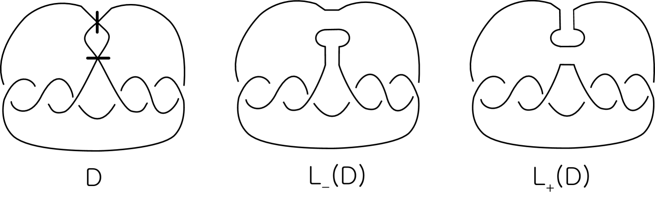
Figure 1: A marked graph diagram and its resolutions

S. J. Lomonaco, Jr. [17] and K. Yoshikawa [25] introduced a method of describing surface-links by marked graph diagrams. Indeed, every surface-link $\mathcal{L}$ is represented by an admissible marked graph diagram $D$. Moreover, if $D$ is an admissible marked graph diagram representing a surface-link $\mathcal{L}$, then we can construct a surface-link $\mathcal{S}(D)$ from $D$ so that $\mathcal{S}(D)$ is equivalent to $\mathcal{L}$. An oriented marked graph diagram is a marked graph diagram in which every edge has an orientation such that each marked vertex looks like (see Fig. 2). If $\mathcal{L}$ is an oriented surface-link, then it is represented by an admissible oriented marked graph diagram. See Section 3 for details. We say that an (oriented) surface-link $\mathcal{L}$ is presented by an (oriented) marked graph diagram $D$ if $\mathcal{L}$ is ambient isotopic to the (oriented) surface-link $\mathcal{S}(D)$.

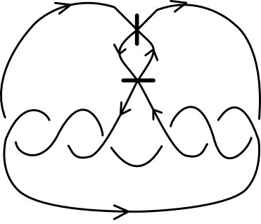
Figure 2: An oriented marked graph diagram

In [25], K. Yoshikawa introduced local moves on marked graph diagrams, nowadays called Yoshikawa moves. In what follows the unoriented Yoshikawa moves mean the deformations $\Omega_{1},\Omega_{2},\Omega_{3},\Omega_{4},\Omega^{\prime}_{4},\Omega_{5}$(Type I) and $\Omega_{6},\Omega^{\prime}_{6},\Omega_{7},\Omega_{8}$ (Type II) on marked graph diagrams without orientations and their all mirror moves shown in Fig. 4, Fig. 4 and Fig. 6. The oriented Yoshikawa moves mean the unoriented Yoshikawa moves with all possible orientations shown in Fig. 5, Fig. 7 and Fig. 13. Then we have

Theorem 1.1 ([11, 23]).

Let $D$ and $D^{\prime}$ be admissible (oriented) marked graph diagrams and let $\mathcal{L}$ and $\mathcal{L}^{\prime}$ be the unoriented (oriented) surface-links presented by $D$ and $D^{\prime}$, respectively. Then the following statements are equivalent.

• $\mathcal{L}$ and $\mathcal{L}^{\prime}$ are equivalent.

• $D$ can be related to $D^{\prime}$ by a finite sequence of unoriented (oriented) Yoshikawa moves.

Using these terminologies, some properties and invariants of surface-links were studied in [2, 5, 6, 12, 13, 14, 15, 22, 25].

Figure 3: A generating set of unoriented Yoshikawa moves

  

  

Figure 4: Unoriented Yoshikawa moves

Figure 5: A generating set of oriented Yoshikawa moves

On many occasions it is necessary to minimize the number of Yoshikawa moves on marked graph diagrams when one checks that a certain function from marked graph diagrams defines a surface-link invariant. A collection $S$ of unoriented (oriented, resp.) Yoshikawa moves is called a generating set of unoriented (oriented, resp.) Yoshikawa moves if any unoriented (oriented, resp.) Yoshikawa move is obtained by a finite sequence of plane isotopies and the moves in the set $S$.

The purpose of this paper is to provide some generating sets of Yoshikawa moves on marked graph diagrams representing unoriented surface-links, and also oriented surface-links. The Main Theorems are the following:

Theorem 1.2.

Let $\mathfrak{S}=\{\Omega_{1},\Omega_{2},\Omega_{3},\Omega_{4},\Omega^{\prime}_{4},\Omega_{5},\Omega_{6},\Omega^{\prime}_{6},\Omega_{7},\Omega_{8}\},$ the set of the moves illustrated in Fig. 4. This is a generating set of unoriented Yoshikawa moves.

Theorem 1.3.

Let $\mathfrak{S}_{1}=\{\Gamma_{1},\Gamma^{\prime}_{1},\Gamma_{2},\Gamma_{3},\Gamma_{4},\Gamma^{\prime}_{4},\Gamma_{5},\Gamma_{6},\Gamma^{\prime}_{6},\Gamma_{7},\Gamma_{8}\},$ the set of the moves illustrated in Fig. 5. This is a generating set of oriented Yoshikawa moves.

Theorem 1.4.

Let $\mathfrak{S}_{2}=\{\Gamma_{1},\Gamma_{1a},\Gamma_{2b},\Gamma_{2c},\Gamma_{3a},\Gamma_{4},\Gamma^{\prime}_{4},\Gamma_{5},\Gamma_{6},\Gamma^{\prime}_{6},\Gamma_{7},\Gamma_{8}\},$ where $\Gamma_{1a},$ $\Gamma_{2b},$ $\Gamma_{2c}$, and $\Gamma_{3a}$ are shown in Fig. 7. This is a generating set of oriented Yoshikawa moves.

We remark that there are two types of oriented Reidemeister moves $\Omega_{3}$ and $\Omega_{3a}$ of type III. One is a cyclic $\Omega_{3}$ (or $\Omega_{3a}$) move of which the central triangle have a cyclic orientation. The other is a non-cyclic $\Omega_{3}$ (or $\Omega_{3a}$) move of which the central triangle does not have a cyclic orientation. Theorem 1.3 gives a generating set $\mathfrak{S}_{1}$ of oriented Yoshikawa moves that contains a cyclic $\Omega_{3}$ move $\Gamma_{3}$. While Theorem 1.4 gives a generating set $\mathfrak{S}_{2}$ of oriented Yoshikawa moves that contains a non-cyclic $\Omega_{3a}$ move $\Gamma_{3a}$ with all three positive crossings.

The rest of this paper is organized as follows. In Section 2, we review minimal generating set of classical Reidemeister moves. In Section 3, we recall the marked graph representation of surface-links. In Section 4, we prove Theorem 1.2. In Section 5, we prove Theorem 1.3 and Theorem 1.4. In Section 6, we discuss independence of certain Yoshikawa moves from the other moves.

2 Minimal generating sets of Reidemeister moves

In this section we recall minimal generating sets of classical Reidemeister moves from [19]. K. Reidemeister introduced three types of local moves on link diagrams and showed that any two link diagrams representing the same link are transformed into each other by a finite sequence of plane isotopies and the local moves as shown in Fig. 6 (cf. [20]), nowadays called Reidemeister moves.

           

Figure 6: Unoriented Reidemeister moves

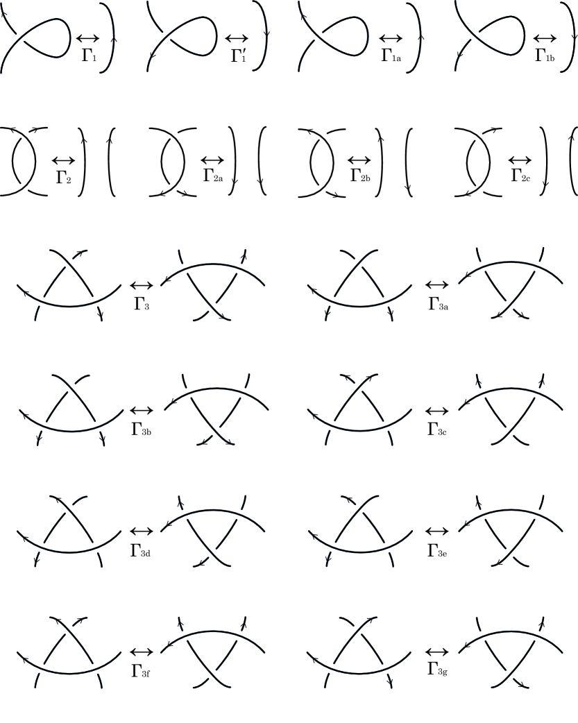
Figure 7: Oriented Reidemeister moves

A collection $S$ of (oriented) Reidemeister moves is called a generating set if any (oriented) Reidemeister move is obtained by a finite sequence of plane isotopies and the moves in the collection $S$. A generating set $S$ is said to be minimal if $S$ does not properly contain any generating set.

We remind the reader that the Reidemeister moves $\Omega_{1},\Omega_{2},\Omega_{3}$ in Fig. 6 is a minimal generating set of unoriented Reidemeister moves, that is, all other Reidemeister moves $\Omega_{1a}$ and $\Omega_{3a}$ in Fig. 6 are obtained by a finite sequence of plane isotopies and the moves $\Omega_{1},\Omega_{2},\Omega_{3}$. We should remark that there are other minimal generating sets of unoriented Reidemeister moves. For example, the Reidemeister moves $\Omega_{1},\Omega_{2},\Omega_{3a}$ in Fig. 6 is also a minimal generating set of unoriented Reidemeister moves, which seems to be considered in many literatures, for example [1, 7, 20].

To deal with oriented link diagrams, depending on orientations of arcs involved in the Reidemeister moves, one may distinguish four different versions of each of the move $\Omega_{1}$, $\Omega_{2}$, $\Omega_{3}$ and $\Omega_{3a}$. For the future use, we here list the oriented Reidemeister moves and name all of them as shown in Fig. 7.

It is obvious that any generating set of oriented Reidemeister moves must contain at least one oriented move of each of the moves $\Omega_{2}$ and $\Omega_{3}$. In [18], Olof-Petter Östlund showed that any generating set of oriented Reidemeister moves has to contain at least two oriented moves of the move $\Omega_{1}$. Hence any generating set of oriented Reidemeister moves has to contain at least four moves. In [19], M. Polyak introduced minimal generating sets of four oriented Reidemeister moves, which include two oriented $\Omega_{1}$ moves, one or two oriented $\Omega_{2}$ move and one oriented $\Omega_{3}$ move (either a cyclic $\Omega_{3}$ move or a non-cyclic $\Omega_{3}$ move):

Theorem 2.1.

[19, Theorem 1.1] Let $D$ and $D^{\prime}$ be two oriented link diagrams in $\mathbb{R}^{2}$ representing the same oriented link. Then one may pass from $D$ to $D^{\prime}$ by a finite sequence of plane isotopies and four oriented Reidemeister moves $\Gamma_{1},\Gamma^{\prime}_{1},\Gamma_{2}$ and $\Gamma_{3}$ in Fig. 7.

Theorem 2.2.

[19, Theorem 1.2] Let $S$ be a set of at most five oriented Reidemeister moves containing the move $\Gamma_{3a}$. Then the set $S$ generates all oriented Reidemeister moves if and only if $S$ contains $\Gamma_{2b}$, $\Gamma_{2c}$ and contains one of the pairs $(\Gamma_{1},\Gamma^{\prime}_{1})$, $(\Gamma_{1},\Gamma_{1a})$, $(\Gamma_{1b},\Gamma^{\prime}_{1})$, or $(\Gamma_{1a},\Gamma_{1b})$.

Remark 2.3.

(1) There are other generating sets for Reidemeister moves. In fact, the set of four oriented Reidemeister moves $\Gamma_{1},\Gamma^{\prime}_{1},\Gamma_{2a}$ and $\Gamma_{3}$ is also a minimal generating set of oriented Reidemeister moves.

(2) Theorem 2.2 implies that any generating set of oriented Reidemeister moves which includes the move $\Gamma_{3a}$ contains at least five moves.

In the rest of the paper, we carefully deal with Yoshikawa moves on marked graph diagrams of surface-links in $\mathbb{R}^{4}$ and provide generating sets of unoriented/oriented Yoshikawa moves, which are analogous to those of unoriented/oriented Reidemeister moves on diagrams of classical links in $\mathbb{R}^{3}$.

3 Marked graph representation of surface-links

In this section, we review marked graph diagrams representing surface-links. A marked graph is a spatial graph $G$ in $\mathbb{R}^{3}$ which satisfies the following:

• $G$ is a finite regular graph with $4$-valent vertices, say $v_{1},v_{2},...,v_{n}$.

• Each $v_{i}$ is a rigid vertex; that is, we fix a rectangular neighborhood $N_{i}$ homeomorphic to $\{(x,y)|-1\leq x,y\leq 1\},$ where $v_{i}$ corresponds to the origin and the edges incident to $v_{i}$ are represented by $x^{2}=y^{2}$.

• Each $v_{i}$ has a marker, which is the interval on $N_{i}$ given by $\{(x,0)|-1\leq x\leq 1\}$.

An orientation of a marked graph $G$ is a choice of an orientation for each edge of $G$ in such a way that every vertex in $G$ looks like . A marked graph $G$ is said to be orientable if it admits an orientation. Otherwise, it is said to be non-orientable. By an oriented marked graph we mean an orientable marked graph with a fixed orientation (see Fig. 2). Two oriented marked graphs are said to be equivalent if they are ambient isotopic in $\mathbb{R}^{3}$ with keeping the rectangular neighborhood, marker and orientation. As usual, a marked graph can be described by a link diagram on $\mathbb{R}^{2}$ with some $4$-valent vertices equipped with markers.

For $t\in\mathbb{R},$ we denote by $\mathbb{R}^{3}_{t}$ the hyperplane of $\mathbb{R}^{4}$ whose fourth coordinate is equal to $t\in\mathbb{R}$, i.e., $\mathbb{R}^{3}_{t}:=\{(x_{1},x_{2},x_{3},x_{4})\in\mathbb{R}^{4}~{}|~{}x_{4}=t\}$. A surface-link $\mathcal{L}\subset\mathbb{R}^{4}=\mathbb{R}^{3}\times\mathbb{R}$ can be described in terms of its cross-sections $\mathcal{L}_{t}=\mathcal{L}\cap\mathbb{R}^{3}_{t},~{}t\in\mathbb{R}$ (cf. [4]). Let $p:\mathbb{R}^{4}\to\mathbb{R}$ be the projection given by $p(x_{1},x_{2},x_{3},x_{4})=x_{4}$. Note that any surface-link can be perturbed to a surface-link $\mathcal{L}$ such that the projection $p:\mathcal{L}\to\mathbb{R}$ is a Morse function with finitely many distinct non-degenerate critical values. More especially, it is well known [7, 9, 10, 17] that any surface-link $\mathcal{L}$ can be deformed into a surface-link $\mathcal{L}^{\prime}$, called a hyperbolic splitting of $\mathcal{L}$, by an ambient isotopy of $\mathbb{R}^{4}$ in such a way that the projection $p:\mathcal{L}^{\prime}\to\mathbb{R}$ satisfies that all critical points are non-degenerate, all the index 0 critical points (minimal points) are in $\mathbb{R}^{3}_{-1}$, all the index 1 critical points (saddle points) are in $\mathbb{R}^{3}_{0}$, and all the index 2 critical points (maximal points) are in $\mathbb{R}^{3}_{1}$.

Let $\mathcal{L}$ be a surface-link and let ${\mathcal{L}^{\prime}}$ be a hyperbolic splitting of $\mathcal{L}.$ Then the cross-section $\mathcal{L}^{\prime}_{0}=\mathcal{L}^{\prime}\cap\mathbb{R}^{3}_{0}$ at $t=0$ is a spatial $4$-valent regular graph in $\mathbb{R}^{3}_{0}$. We give a marker at each $4$-valent vertex (saddle point) that indicates how the saddle point opens up above as illustrated in Fig. 8.

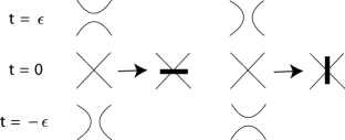
Figure 8: Marking of a vertex

The resulting marked graph $G$ is called a marked graph presenting $\mathcal{L}$. As usual, $G$ is described by a diagram $D$ in $\mathbb{R}^{2}$, which is a generic projection on $\mathbb{R}^{2}$ of $G$ with over/under crossing information for each double point, as in a classical link diagram, such that the restriction to a small rectangular neighborhood of each marked vertex is a homeomorphism. Such a diagram $D$ is called a marked graph diagram (or ch-diagram (cf. [22])) presenting $\mathcal{L}$.

When $\mathcal{L}$ is an oriented surface-link, we choose an orientation for each edge of $\mathcal{L}^{\prime}_{0}$ that coincides with the induced orientation on the boundary of $\mathcal{L}^{\prime}\cap\mathbb{R}^{3}\times(-\infty,0]$ by the orientation of $\mathcal{L}^{\prime}$ inherited from the orientation of $\mathcal{L}$. The resulting oriented marked graph diagram $D$ is called an oriented marked graph diagram presenting the oriented surface-link $\mathcal{L}$.

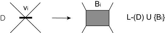
Figure 9: A band attached to $L_{-}(D)$ at $v_{i}$

Now let $D$ be a given admissible marked graph diagram with marked vertices $v_{1},\ldots,v_{n}$. We define a surface $F(D)\subset\mathbb{R}^{3}\times[-1,1]$ by

$$(\mathbb{R}^{3}_{t},F(D)\cap\mathbb{R}^{3}_{t})=\left\{\begin{array}[]{ll}(\mathbb{R}^{3},L_{+}(D))&\hbox{for $0<t\leq 1$,}\\ \bigg{(}\mathbb{R}^{3},L_{-}(D)\cup\bigg{(}\overset{n}{\underset{i=1}{\cup}}B_{i}\bigg{)}\bigg{)}&\hbox{for $t=0$,}\\ (\mathbb{R}^{3},L_{-}(D))&\hbox{for $-1\leq t<0$,}\\ \end{array}\right.$$

where $B_{i}(i=1,\ldots,n)$ is a band attached to $L_{-}(D)$ at the marked vertex $v_{i}$ as shown in Fig. 9. We call $F(D)$ the proper surface associated with $D$. Since $D$ is admissible, we can obtain a surface-link from $F(D)$ by attaching trivial disks in $\mathbb{R}^{3}\times[1,\infty)$ and another trivial disks in $\mathbb{R}^{3}\times(-\infty,1]$. We denote this surface-link by $\mathcal{S}(D)$, and call it the surface-link associated with $D$. It is known that the isotopy type of $\mathcal{S}(D)$ does not depend on choices of trivial disks (cf. [7, 10]). It is straightforward from the construction of $\mathcal{S}(D)$ that $D$ is a marked graph diagram presenting $\mathcal{S}(D)$.

It is known that $D$ is orientable if and only if $F(D)$ is an orientable surface. When $D$ is oriented, the resolutions $L_{-}(D)$ and $L_{+}(D)$ have orientations induced from the orientation of $D$, and we assume $F(D)$ is oriented so that the induced orientation on $L_{+}(D)=\partial F(D)\cap\mathbb{R}^{3}_{1}$ matches the orientation of $L_{+}(D)$.

Theorem 1.1 in Section 1 shows that a surface-link is completely described by its marked graph diagram modulo unoriented Yoshikawa’s moves, and also shows that an oriented surface-link is completely described by its oriented marked graph diagram modulo oriented Yoshikawa’s moves.

4 Proof of Theorem 1.2

To prove Theorem 1.2, it suffices to show that the mirror moves in Fig. 4 and the Reidemeister moves $\Omega_{1a}$ and $\Omega_{3a}$ in Fig. 6 are generated by the $10$ moves in the set $\mathfrak{S}$ in Theorem 1.2. This is going to be done in several steps. We begin with the following

Lemma 4.1.

The move $\Omega_{4a}$ is realized by $\Omega_{2}$, $\Omega_{4}$ and plane isotopies. The move $\Omega^{\prime}_{4a}$ is realized by $\Omega_{2}$, $\Omega^{\prime}_{4}$ and plane isotopies.

Proof.

See Fig. 11. $\square$

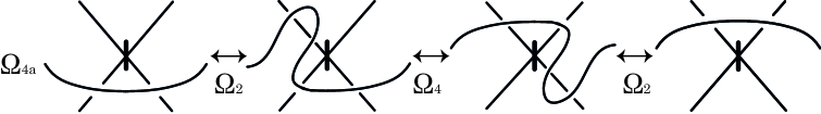
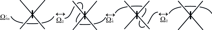
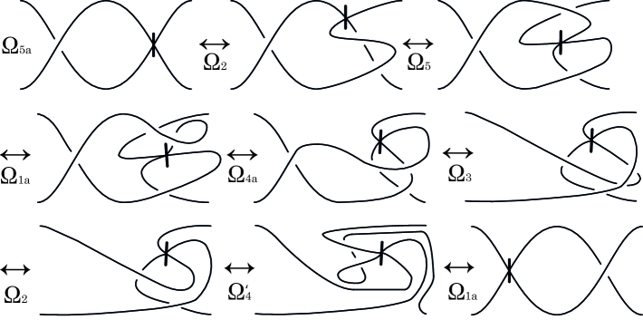
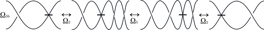
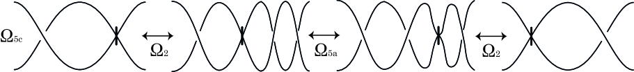
Figure 10: Mirror moves of $\Omega_{4}$ and $\Omega^{\prime}_{4}$

Figure 11: Mirror moves of $\Omega_{5}$

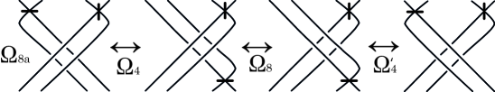
Figure 12: Mirror move of $\Omega_{8}$

Lemma 4.2.

The move $\Omega_{5a}$ is realized by $\Omega_{1a}$, $\Omega_{2}$, $\Omega_{3}$, $\Omega^{\prime}_{4}$, $\Omega_{4a}$, $\Omega_{5}$ and plane isotopies. The move $\Omega_{5b}$ is realized by $\Omega_{2}$, $\Omega_{5}$ and plane isotopies. The move $\Omega_{5c}$ is realized by $\Omega_{2}$, $\Omega_{5a}$ and plane isotopies.

Proof.

See Fig. 11. $\square$

Lemma 4.3.

The move $\Omega_{8a}$ is realized by $\Omega_{4}$, $\Omega^{\prime}_{4}$, $\Omega_{8}$ and plane isotopies.

Proof.

See Fig. 12. $\square$

Proof of Theorem 1.2. Let $M$ be a move of the unoriented Yoshikawa moves. Note that the three Reidemeister moves $\Omega_{1},\Omega_{2},\Omega_{3}$ generate all unoriented Reidemeister moves and so do $\Omega_{1a}$ and $\Omega_{3a}$ (cf. Section 2). From Lemmas 4.1, 4.2 and 4.3, it is seen that $M$ lies in the set $\mathfrak{S}$ in Theorem 1.2, or $M$ can be generated by the moves lie in $\mathfrak{S}$. This completes the proof of Theorem 1.2. $\Box$

Remark 4.4.

There are minimal generating sets of classical Reidemeister moves other than $\{\Omega_{1},\Omega_{2},\Omega_{3}\}$. For example, $\{\Omega_{1a},\Omega_{2},\Omega_{3a}\}$. Indeed, replacing any generating set of Reidemeister moves with the moves $\Omega_{1},\Omega_{2},\Omega_{3}$ yields a generating set of unoriented Yoshikawa moves. This fact and Lemmas 4.1-4.3 enable us to do that we can choose a generating set of unoriented Yoshikawa moves other than one given in Theorem 1.2. For example, it is easily seen that $\{\Omega_{1a},\Omega_{2},\Omega_{3a},\Omega_{4},\Omega^{\prime}_{4},\Omega_{5},\Omega_{6},$ $\Omega^{\prime}_{6},$ $\Omega_{7},\Omega_{8}\}$ and $\{\Omega_{1a},\Omega_{2},\Omega_{3a},\Omega_{4a},\Omega_{4b},\Omega_{5},\Omega_{6},\Omega^{\prime}_{6},\Omega_{7},\Omega_{8}\}$ are also generating sets of unoriented Yoshikawa moves.

5 Proof of Theorem 1.3 and Theorem 1.4

We remind that the oriented Yoshikawa moves are the moves $\Omega_{i}(i=1,2,\ldots,8),$ $\Omega^{\prime}_{4},$ $\Omega^{\prime}_{6}$ in Fig. 4, $\Omega_{4a},\Omega^{\prime}_{4a},\Omega_{5a},$ $\Omega_{5b},$ $\Omega_{5c},\Omega_{8a}$ in Fig. 4 and Fig. 6 with all possible orientations. On the other hand, by virtue of Theorem 1.2, we see that any such an oriented Yoshikawa move is generated by plane isotopies and some moves lie in the generating set $\mathfrak{S}=\{\Omega_{1},\Omega_{2},\Omega_{3},\Omega_{4},\Omega^{\prime}_{4},\Omega_{5},\Omega_{6},\Omega^{\prime}_{6},\Omega_{7},\Omega_{8}\}$ of 10 Yoshikawa moves with all possible orientations. In Section 2, we have discussed the oriented Reidemeister moves $\Gamma_{1},\Gamma_{2},\Gamma_{3}$ (see Fig. 7). Now it is easily seen that all possible Yoshikawa moves $\Omega_{4},\ldots,\Omega_{8},\Omega^{\prime}_{4},\Omega^{\prime}_{6}$ with orientations are the oriented moves $\Gamma_{4},\ldots,\Gamma_{8},\Gamma^{\prime}_{4},\Gamma^{\prime}_{6}$ in Fig. 5 and the moves $\Gamma_{4a},\Gamma^{\prime}_{4a},\Gamma_{6a},\Gamma^{\prime}_{6a},\Gamma_{7a},\Gamma_{8a},\Gamma_{8b},\Gamma_{8c}$ shown in Fig. 13. We note that the move $\Gamma_{5}$ with reverse orientation is the move $\Gamma_{5}$ itself.

  

  

  

  

Figure 13: Oriented Yoshikawa moves of type $4$-$8$

We first prove Theorem 1.3 and then Theorem 1.4. The proof of Theorem 1.3 consists of showing that all oriented Yoshikawa moves in Fig. 13 can be realized by a finite sequence of plane isotopies, the moves $\Gamma_{i}(1\leq i\leq 8)$ and $\Gamma_{i}^{\prime}(i=1,4,6)$. This will proceed in several lemmas as the followings.

Lemma 5.1.

The move $\Gamma_{4a}$ is realized by a finite sequence of the moves $\Gamma_{2a},$ $\Gamma_{2b},$ $\Gamma_{3b},$ $\Gamma_{3c},$ $\Gamma_{4},$ $\Gamma_{5}$ and plane isotopies. The move $\Gamma^{\prime}_{4a}$ is realized by a finite sequence of the moves $\Gamma_{2},$ $\Gamma_{2b},$ $\Gamma_{3e},$ $\Gamma_{3f},$ $\Gamma^{\prime}_{4},$ $\Gamma_{5}$ and plane isotopies.

Proof.

See Fig. 14. $\square$

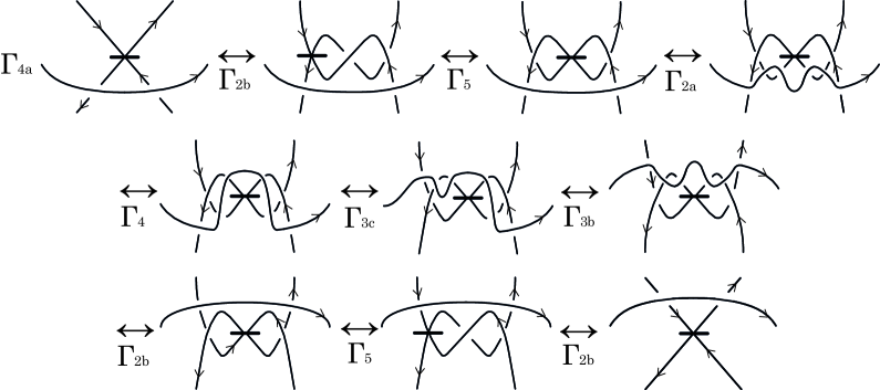
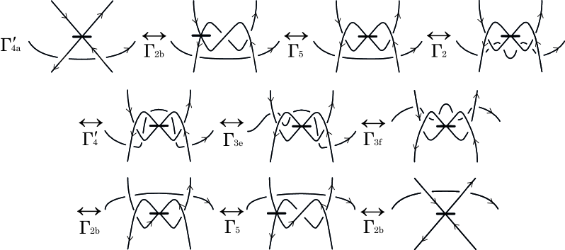
Figure 14: Oriented Yoshikawa moves $\Gamma_{4a}$ and $\Gamma^{\prime}_{4a}$

Lemma 5.2.

Let $\Gamma_{5a}$ denote the oriented Yoshikawa move of type 5 shown in Fig. 15. Then it is realized by a finite sequence of the moves $\Gamma^{\prime}_{1},$ $\Gamma_{1b},$ $\Gamma_{2a},$ $\Gamma_{2b},$ $\Gamma_{3b},$ $\Gamma_{4},$ $\Gamma^{\prime}_{4},$ $\Gamma_{5}$ and plane isotopies.

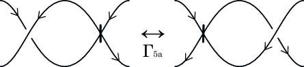
Figure 15: Oriented Yoshikawa move $\Gamma_{5a}$

Proof.

See Fig. 16. $\square$

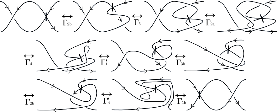
Figure 16: A realization of $\Gamma_{5a}$

Lemma 5.3.

The move $\Gamma_{6a}$ is realized by a finite sequence of the moves $\Gamma^{\prime}_{1},$ $\Gamma_{1b},$ $\Gamma_{2},$ $\Gamma_{2a},$ $\Gamma_{2b},$ $\Gamma_{3b},$ $\Gamma_{4},$ $\Gamma^{\prime}_{4},$ $\Gamma_{5}$, $\Gamma_{6}$ and plane isotopies. The move $\Gamma^{\prime}_{6a}$ is realized by a finite sequence of the moves $\Gamma^{\prime}_{1},$ $\Gamma_{5},$ $\Gamma^{\prime}_{6}$.

Proof.

It follows from Fig. 17 that the moves $\Gamma_{6a}$ is realized by the moves $\Gamma^{\prime}_{1},$ $\Gamma_{5a},$ $\Gamma_{6}$ and plane isotopies. By Lemma 5.2, the move $\Gamma_{5a}$ is realized by a finite sequence of the moves $\Gamma^{\prime}_{1},$ $\Gamma_{1b},$ $\Gamma_{2},$ $\Gamma_{2a},$ $\Gamma_{2b},$ $\Gamma_{3b},$ $\Gamma_{4},$ $\Gamma^{\prime}_{4},$ $\Gamma_{5}$ and plane isotopies. This gives the assertion for $\Gamma_{6a}$. It is immediate from Fig. 17 that the move $\Gamma^{\prime}_{6a}$ is realized by a finite sequence of the moves $\Gamma^{\prime}_{1},$ $\Gamma_{5},$ $\Gamma^{\prime}_{6}$. This completes the proof. $\square$

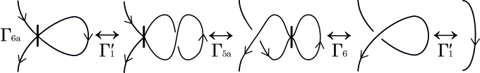
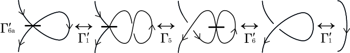
Figure 17: Oriented Yoshikawa move $\Gamma_{6a}$ and $\Gamma^{\prime}_{6a}$

Lemma 5.4.

The move $\Gamma_{7a}$ is realized by a finite sequence of the moves $\Gamma^{\prime}_{1},$ $\Gamma_{1a},$ $\Gamma_{1b},$ $\Gamma_{2},$ $\Gamma_{2b},$ $\Gamma_{2c},$ $\Gamma_{3b},$ $\Gamma_{4},$ $\Gamma^{\prime}_{4},$ $\Gamma_{4a},$ $\Gamma_{5},$ $\Gamma_{5a},$ $\Gamma_{7}$ and plane isotopies.

Proof.

It follows from Fig. 19 that the move $\Gamma_{7a}$ is realized by a finite sequence of the moves $\Gamma_{1a},$ $\Gamma^{\prime}_{1},$ $\Gamma_{2b},$ $\Gamma_{2c},$ $\Gamma_{4a},$ $\Gamma^{\prime}_{4},$ $\Gamma_{5},$ $\Gamma_{5a},$ $\Gamma_{7}$ and plane isotopies. By Lemma 5.2, the move $\Gamma_{5a}$ can be replaced with the moves $\Gamma^{\prime}_{1},$ $\Gamma_{1b},$ $\Gamma_{2},$ $\Gamma_{2a},$ $\Gamma_{2b},$ $\Gamma_{3b},$ $\Gamma_{4},$ $\Gamma^{\prime}_{4},$ $\Gamma_{5}$. This gives the assertion of the lemma. $\square$

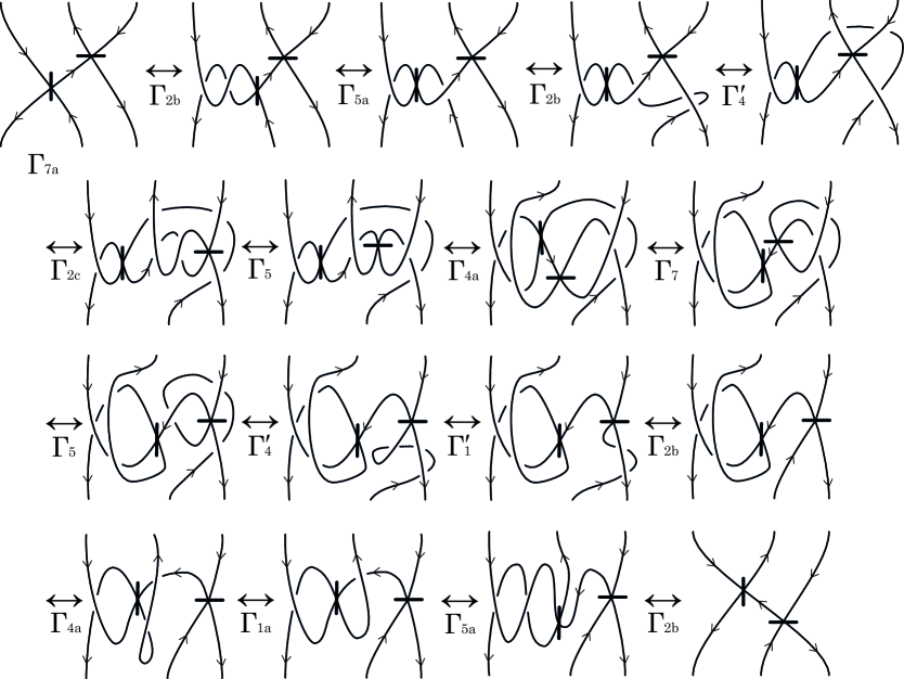
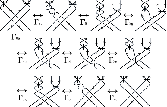
Figure 18: Oriented Yoshikawa move $\Gamma_{7a}$

Figure 19: Oriented Yoshikawa move $\Gamma_{8a}$

Lemma 5.5.

The move $\Gamma_{8a}$ is realized by a finite sequence of the moves $\Gamma_{2c},$ $\Gamma_{3c},$ $\Gamma_{3g},$ $\Gamma_{3e},$ $\Gamma_{5},$ $\Gamma_{8}$ and plane isotopies. The move $\Gamma_{8b}$ is realized by a finite sequence of the moves $\Gamma_{2b},$ $\Gamma_{3c},$ $\Gamma_{3e},$ $\Gamma_{3g},$ $\Gamma^{\prime}_{1},$ $\Gamma_{1b},$ $\Gamma_{2},$ $\Gamma_{2a},$ $\Gamma_{2b},$ $\Gamma_{3b},$ $\Gamma_{4},$ $\Gamma^{\prime}_{4},$ $\Gamma_{5}$, $\Gamma_{8a}$ and plane isotopies. The move $\Gamma_{8c}$ is realized by a finite sequence of the moves $\Gamma_{2b},$ $\Gamma_{3c},$ $\Gamma_{3e},$ $\Gamma_{3g},$ $\Gamma^{\prime}_{1},$ $\Gamma_{1b},$ $\Gamma_{2},$ $\Gamma_{2a},$ $\Gamma_{2b},$ $\Gamma_{3b},$ $\Gamma_{4},$ $\Gamma^{\prime}_{4},$ $\Gamma_{5}$, $\Gamma_{8a}$ and plane isotopies.

Proof.

It is immediate from Fig. 19 that the move $\Gamma_{8a}$ is realized by a finite sequence of the moves $\Gamma_{2c},$ $\Gamma_{3c},$ $\Gamma_{3g},$ $\Gamma_{3e},$ $\Gamma_{5},$ $\Gamma_{8}$ and plane isotopies. This gives the assertion for $\Gamma_{8a}$. Now it follows from Fig. 21 that the move $\Gamma_{8b}$ is realized by a finite sequence of the moves $\Gamma_{2b},$ $\Gamma_{3c},$ $\Gamma_{3e},$ $\Gamma_{3g},$ $\Gamma_{5a}$, $\Gamma_{8a}.$ By Lemma 5.2, the move $\Gamma_{5a}$ can be replaced with the moves $\Gamma^{\prime}_{1},$ $\Gamma_{1b},$ $\Gamma_{2},$ $\Gamma_{2a},$ $\Gamma_{2b},$ $\Gamma_{3b},$ $\Gamma_{4},$ $\Gamma^{\prime}_{4},$ $\Gamma_{5}$. This yields the assertion for $\Gamma_{8b}$. Similarly, we obtain the assertion for the move $\Gamma_{8c}$ (see Fig. 21). This completes the proof. $\square$

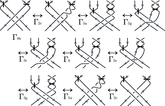
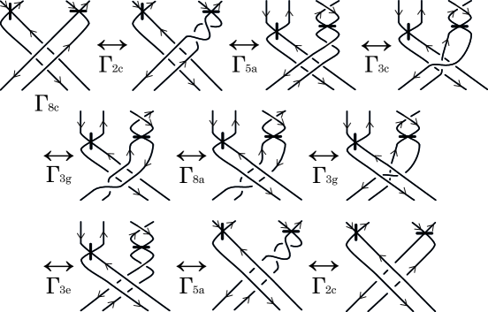
Figure 20: Oriented Yoshikawa move $\Gamma_{8b}$

Figure 21: Oriented Yoshikawa move $\Gamma_{8b}$ and $\Gamma_{8c}$

Now let us complete the proof of Theorem 1.3 and Theorem 1.4.

Proof of Theorem 1.3. Let $M$ be a move of the oriented Yoshikawa moves. From Theorem 1.2, we see that $M$ without orientation is generated by the only $10$ unoriented moves $\Omega_{i},\Omega^{\prime}_{i}\in\mathfrak{S}$. This gives that $M$ is generated by the 10 moves $\Omega_{1},\Omega_{2},\Omega_{3},\Omega_{4},\Omega^{\prime}_{4}$, $\Omega_{5}$, $\Omega_{6},\Omega^{\prime}_{6},\Omega_{7},\Omega_{8}$ with orientations. In Fig. 5, Fig. 7 and Fig. 13, these 10 moves with all possible orientations are found. From Theorem 2.1, we see that the classical Reidemeister moves $\Omega_{1},\Omega_{2},\Omega_{3}$ with orientation are generated by the moves $\Gamma_{1},\Gamma^{\prime}_{1},\Gamma_{2}$ and $\Gamma_{3}$. For other oriented moves, it is seen from Lemmas 5.1, 5.3, 5.4, 5.5 that the moves are realized by a finite sequence of oriented moves $\Gamma_{i}$ and $\Gamma^{\prime}_{i}$ listed in $\mathfrak{S}_{1}$. This completes the proof of Theorem 1.3. $\Box$

Proof of Theorem 1.4. Let $M$ be a move of the oriented Yoshikawa moves. In the proof of Theorem 1.3, we see that $M$ is generated by the 10 moves $\Omega_{1},\Omega_{2},\Omega_{3},$ $\Omega_{4},$ $\Omega^{\prime}_{4}$, $\Omega_{5}$, $\Omega_{6},\Omega^{\prime}_{6},\Omega_{7},\Omega_{8}$ with orientations in Fig. 5, Fig. 7 and Fig. 13. From Theorem 2.2, we see that the five oriented Reidemeister moves $\Gamma_{1},\Gamma^{\prime}_{1},\Gamma_{2b},\Gamma_{2c},\Gamma_{3a}$ generate all oriented Reidemeister moves. Thus the assertion follows from the previous theorem 1.3 at once. This completes the proof of Theorem 1.4. $\Box$

Remark 5.6.

There are various generating sets of classical oriented Reidemeister moves other than $\{\Gamma_{1},\Gamma^{\prime}_{1},\Gamma_{2b},\Gamma_{2c},\Gamma_{3a}\}$ contianing the non-cyclic $\Omega_{3a}$ move $\Gamma_{3a}$ (see Theorem 2.2). Replacing any generating set of oriented Reidemeister moves with the moves $\Gamma_{1},\Gamma^{\prime}_{1},\Gamma_{2b},\Gamma_{2c},\Gamma_{3a}$ yields a generating set of oriented Yoshikawa moves. This fact and Lemmas 5.1-5.5 enable us to show that we can choose a generating set of oriented Yoshikawa moves other than ones given in Theorem 1.3 and Theorem 1.4. For example, it is easily seen from Theorem 2.2 that $\{\Gamma_{1},\Gamma_{1a},\Gamma_{2b},\Gamma_{2c},\Gamma_{3a},\Gamma_{4},\Gamma^{\prime}_{4},\Gamma_{5}$, $\Gamma_{6},\Gamma^{\prime}_{6},\Gamma_{7},\Gamma_{8}\}$, $\{\Gamma_{1b},\Gamma^{\prime}_{1},\Gamma_{2b},\Gamma_{2c},\Gamma_{3a},\Gamma_{4},\Gamma^{\prime}_{4},\Gamma_{5}$, $\Gamma_{6},\Gamma^{\prime}_{6},\Gamma_{7},\Gamma_{8}\}$ and $\{\Gamma_{1a},\Gamma_{1b},\Gamma_{2b},\Gamma_{2c},$
$\Gamma_{3a},\Gamma_{4},\Gamma^{\prime}_{4},\Gamma_{5}$, $\Gamma_{6},\Gamma^{\prime}_{6},\Gamma_{7},\Gamma_{8}\}$ are all generating sets of oriented Yoshikawa moves.

6 Independence of Yoshikawa moves

For classical links in $\mathbb{R}^{3}$, it is well known that each Reidemeister move cannot be generated by the other two type moves, that is, a Reidemeister move is independent from the other types (cf. [16, Appendix A]).

For Roseman moves on broken surface diagrams of surface-links in $\mathbb{R}^{4},$ there also exist analogue results. Indeed, let $\mathcal{L}$ be a surface-link in $\mathbb{R}^{4}$ and let $\pi:\mathbb{R}^{4}\to\mathbb{R}^{3}$ be the projection defined by $\pi(x_{1},x_{2},x_{3},x_{4})=(x_{1},x_{2},x_{3}).$ By a slight perturbation of $\mathcal{L}$ if necessary, we may assume that the restriction $\pi|_{\mathcal{L}}:\mathcal{L}\to\mathbb{R}^{3}$ is a generic map, i.e., the sigularities of $\pi|_{\mathcal{L}}$ consist of double point curves and isolated triple or branch points. The image $\pi(\mathcal{L})$ in which the lower sheets are consistently removed along the double point curves is called a broken surface diagram of $\mathcal{L}$. For more details, see [3, 7]. In [21], D. Roseman proved that two surface-links are equivalent if and only if their broken surface diagrams are transformed into each other by applying a finite number of seven types of local moves on broken surface diagrams which are called the Roseman moves. In [24], T. Yashiro proved that Roseman move of type 2 can be generated by the moves of type 1 and type 4. Recently, K. Kawamura showed that Roseman move of type 1 can be generated by the moves of type 2 and type 3, and for any $i(i=3,4,5,6,7)$, Roseman move of type i cannot be generated by the other six types, that is, Roseman move of type $i$ is independent from the other six type moves [8].

For Yoshikawa moves on marked graph diagrams, it is natural to ask whether each Yoshikawa move is independent from the other moves. In Theorem 1.2, we have proved that $\mathfrak{S}=\{\Omega_{1},\ldots,\Omega_{8},\Omega^{\prime}_{4},\Omega^{\prime}_{6}\}$ is a generating set of all unoriented Yoshikawa moves. From now on we shall discuss the independence of each Yoshikawa move in $\mathfrak{S}$ from the other moves in $\mathfrak{S}$.

Theorem 6.1.

The Yoshikawa move $\Omega_{1}$ is independent from the other moves in $\mathfrak{S}$.

Proof.

It is clear that all moves in $\mathfrak{S}$ except $\Omega_{1}$ keep the parity of the number of crossings and the move $\Omega_{1}$ changes the number of crossing by one and so does the parity. This gives that $\Omega_{1}$ cannot be realized by the moves in $\mathfrak{S}-\{\Omega_{1}\}$. $\square$

Theorem 6.2.

The Yoshikawa move $\Omega_{2}$ is independent from the other moves in $\mathfrak{S}$.

Proof.

Let $D=D_{1}\cup D_{2}$ be a two component marked graph diagram in $\mathbb{R}^{2}$. By $|D|=|D_{1}|\cup|D_{2}|$ we denote the $4$-valent graph in $\mathbb{R}^{2}$ obtained from $D$ by removing markers and by assuming crossings to be verticess of valency $4$. Define

$$s(D)=\begin{cases}0&\text{if $|D_{1}|\cap|D_{2}|=\emptyset$},\\ 1&\text{otherwise}.\end{cases}$$

Then it is easily seen that $s(D)$ is invariant under all moves in $\mathfrak{S}$ except $\Omega_{2}$. Now let $D=\bigcirc~{}\bigcirc$ and $D^{\prime}=\lx@xy@svg{\hbox{\raise 0.0pt\hbox{\kern 11.38104pt\hbox{{\hbox{\kern-11.38104pt\raise 0.0pt\hbox{\hbox{\kern 0.0pt\raise-17.69052pt\hbox{\hbox{\vbox{\vskip 11.38104pt\hbox to22.76208pt{\hfill\lx@xy@buildcircle@\hfill}\vskip 11.38104pt}}}}}}}\ignorespaces\hbox{\hbox{\kern 0.0pt\raise 0.0pt\hbox{{}{{}{}}{{}{}{}\lx@xy@spline@}{}}}}\ignorespaces\hbox{\hbox{\kern 0.0pt\raise 0.0pt\hbox{{}{{}{}}{{}{}{}\lx@xy@spline@}{}}}}\ignorespaces\hbox{\hbox{\kern 0.0pt\raise 0.0pt\hbox{{}{{}{}}{{}{}{}\lx@xy@spline@}{}}}}\ignorespaces\hbox{\hbox{\kern 0.0pt\raise 0.0pt\hbox{{}{{}{}}{{}{}{}\lx@xy@spline@}{}}}}}}}}$. Then $D$ and $D^{\prime}$ are two diagrams of the trivial $S^{2}$-link with two components, and $s(D)=0$ and $s(D^{\prime})=1$. This gives that $s(D)$ is not an invariant of the move $\Omega_{2}$. Hence $\Omega_{2}$ cannot be realized by the moves in $\mathfrak{S}-\{\Omega_{2}\}$. $\square$

Let $D=D_{1}\cup D_{2}\cup D_{3}$ be a marked graph diagram in $\mathbb{R}^{2}$ with three components. Let $T(D)=\{p(D_{1}),p(D_{2}),p(D_{3})\}$ be the non-ordered triple of numbers with $p(D_{i})\in\{0,1\}$ defined as follows. For each $i=1,2,3$, the component $D_{i}$ tiles $\mathbb{R}^{2}$ into regions which admit a checkboard coloring. We color the unbounded region to be white. Let $B(D_{i})$ denote the set of all black regions and let $n(D_{i})$ be the number of crossings of two components different from $D_{i}$ and lie in $B(D_{i})$. We define $p(D_{i})=n(D_{i})\pmod{2}$. Then we have the following:

Lemma 6.3.

The non-ordered triple $T(D)=\{p(D_{1}),p(D_{2}),p(D_{3})\}$ is invariant under all moves in $\mathfrak{S}$ except the move $\Omega_{3}$.

Proof.

For all moves in $\mathfrak{S}$ except the move $\Omega_{3}$, it is easily seen that the moves involves only one or two components. This straightforwardly gives that the moves contributing the value $T(D)$ are performed in a region with the same color. Since the all moves contains even number of crossings, the parity of $n(D_{i})$ does not changed for each $i=1,2,3$. This completes the proof. $\square$

Theorem 6.4.

The Yoshikawa moves $\Omega_{3}$ is independent from the other moves in $\mathfrak{S}$.

Proof.

Let $D=D_{1}\cup D_{2}\cup D_{3}$ and $D^{\prime}=D^{\prime}_{1}\cup D^{\prime}_{2}\cup D^{\prime}_{3}$ be the diagrams of the trivial $S^{2}$-link with three components as shown in Fig. 22.

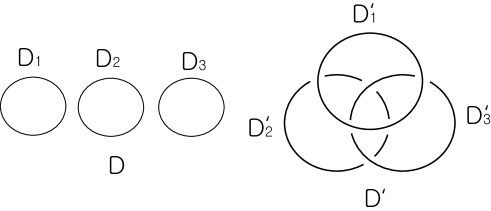
Figure 22: Diagrams of the trivial $S^{2}$-link with three components

Then it is easily seen that $p(D_{1})=p(D_{2})=p(D_{3})=1$ and so $T(D)=\{1\}$. But $p(D^{\prime}_{1})=p(D^{\prime}_{2})=p(D^{\prime}_{3})=0$ and so $T(D^{\prime})=\{0\}$. By Lemma 6.3, $D$ cannot be transformed into $D^{\prime}$ by using a sequence of the moves in $\mathfrak{S}-\{\Omega_{3}\}$. This concludes that the move $\Omega_{3}$ is independent from the moves in $\mathfrak{S}-\{\Omega_{3}\}$. $\square$

Theorem 6.5.

[5, Corollary 6.3] The Yoshikawa move $\Omega_{4}$ and $\Omega^{\prime}_{4}$ are independent from the moves in $\mathfrak{S}-\{\Omega_{4},\Omega^{\prime}_{4}\}$.

Theorem 6.6.

The Yoshikawa move $\Omega_{6}$ is independent from the other moves in $\mathfrak{S}$. The Yoshikawa move $\Omega^{\prime}_{6}$ is independent from the other moves in $\mathfrak{S}$.

Proof.

Let $D$ be a marked graph diagram and let $\mu_{+}(D)$ and $\mu_{-}(D)$ denote the numbers of components of the positive resolution $L_{+}(D)$ and the negative resolution $L_{-}(D)$ of $D$, respectively. Then it is easily seen that $\mu_{+}(D)$ is invariant under all moves in $\mathfrak{S}$ except $\Omega_{6}$ and $\mu_{-}(D)$ is invariant under all moves in $\mathfrak{S}$ except $\Omega^{\prime}_{6}$. But, the move $\Omega_{6}$ changes the number of components of $L_{+}(D)$ by one, and $\Omega^{\prime}_{6}$ changes the number of components of $L_{-}(D)$ by one. This implies the assertions. $\square$

Theorem 6.7.

[6, Theorem 5.4] The Yoshikawa move $\Omega_{7}$ is independent from the other moves in $\mathfrak{S}$.

Let $D$ be a marked graph diagram and let $\tilde{D}$ be a classical link diagram obtained form $D$ by replacing each marked vertex to the crossing $\lx@xy@svg{\hbox{\raise 0.0pt\hbox{\kern 14.2263pt\hbox{\ignorespaces{\hbox{\lx@xy@drawline@}}\ignorespaces{\hbox{\lx@xy@drawline@}}\ignorespaces{\hbox{\lx@xy@drawline@}}}}}}.$ Let $\sharp D$ denote the number of the components of $\tilde{D}$. Then it is obvious that $\sharp D$ is an invariant of $D$ under all Yoshikawa moves in $\mathfrak{S}$ except the move $\Omega_{7}$. It is not difficult to find two marked graph diagrams $D$ and $D^{\prime}$ that are differ by a single $\Omega_{7}$ and satisfy $\sharp D\not=\sharp D^{\prime}$. This gives an alternative proof of Theorem 6.7.

Corollary 6.8.

Let $\Gamma$ be an oriented Yoshikawa move in $\mathfrak{S}_{1}-\{\Gamma_{5},\Gamma_{8}\}$ ($\mathfrak{S}_{2}-\{\Gamma_{5},\Gamma_{8}\}$, resp.). Then $\Gamma$ is independent from the other oriented moves in $\mathfrak{S}_{1}$ ($\mathfrak{S}_{2}$. resp.).

Proof.

Suppose that $\Gamma$ is realized by a finite sequence $M_{1},M_{2},\ldots,M_{k}$ with $k\geq 1$ and $M_{i}\in\mathfrak{S}_{1}-\{\Gamma\}$ ($\mathfrak{S}_{2}-\{\Gamma\}$. resp.) for all $1\leq i\leq k$. Let $\overline{\Gamma}$ and $\overline{M}_{i}$ be the moves $\Gamma$ and $M_{i}$ forgetting the orientations, respectively. Then we see that $\overline{\Gamma}$ is realized by the finite sequence $\overline{M}_{1},\overline{M}_{2},\ldots,\overline{M}_{k}$. Since $\overline{\Gamma}\in\mathfrak{S}-\{\Omega_{5},\Omega_{8}\}$ and $\overline{M}_{i}\in\mathfrak{S}-\{\overline{\Gamma}\}$, we have a contradiction. This completes the proof. $\square$

We now close this section with the following four questions. If the answers of these questions are all affirmative, then the generating sets $\mathfrak{S}$, $\mathfrak{S}_{1}$ and $\mathfrak{S}_{2}$ are all minimal.

Question 1. Is the Yoshikawa move $\Omega_{4}$ independent from the other moves in $\mathfrak{S}$?

Question 2. Is the Yoshikawa move $\Omega^{\prime}_{4}$ independent from the other moves in $\mathfrak{S}$?

Question 3. Is the Yoshikawa moves $\Omega_{5}$ independent from the other moves in $\mathfrak{S}$?

Question 4. Is the Yoshikawa move $\Omega_{8}$ independent from the other moves in $\mathfrak{S}$?

References

- [1] J. W. Alexander and G. B. Briggs, On types of knotted curves, Ann. of Math. 28 (1926/1927), 562–586.
- [2] M. Asada, An unknotting sequence for surface-knots represented by ch-diagrams and their genera, Kobe J. Math. 18 (2001), 163–180.
- [3] J. S. Carter and M. Saito, Knotted surfaces and their diagrams, Mathematical Surveys and Monographs 55, AMS Providence, RI, 1998.
- [4] R. H. Fox, A quick trip through knot theory, in Toplogy of -manifolds and Related Topics, (Prentice-Hall, Inc., Englewood Cliffs, N.J., 1962), 120–167.
- [5] Y. Joung, S. Kamada and S. Y. Lee, Applying Lipson’s state models to marked graph diagrams of surface-links, arXiv:1411.5740.
- [6] Y. Joung, J. Kim and S. Y. Lee, Ideal coset invariants for surface-links in , J. Knot Theory Ramifications 22 (2013), No. 9, 1350052(25 pages).
- [7] S. Kamada, Braid and Knot Theory in dimension Four, Mathematical Surveys and Monographs Vol. 95, (American Mathematical Society, 2002).
- [8] K. Kawamura, On relationship between seven types of Roseman moves, preprint.
- [9] A. Kawauchi, A survey of knot theory, (Birkhäuser, 1996).
- [10] A. Kawauchi, T. Shibuya, S. Suzuki, Descriptions on surfaces in four-space, I; Normal forms, Math. Sem. Notes Kobe Univ. 10(1982), 75–125.
- [11] C. Kearton and V. Kurlin, All 2-dimensional links in 4-space live inside a universal 3-dimensional polyhedron, Algebraic & Geometric Topology 8 (2008), 1223–1247.
- [12] J. Kim, Y. Joung and S. Y. Lee, On the Alexander biquandles of oriented surface-links via marked graph diagrams, J. Knot Theory Ramifications 23 (2014), No. 7, 1460007 (26 pages).
- [13] S. Y. Lee, Invariants of surface links in via classical link invariants. Intelligence of low dimensional topology 2006, 189–196, Ser. Knots Everything, 40, (World Sci. Publ., Hackensack, NJ, 2007).
- [14] S. Y. Lee, Invariants of surface links in via skein relation, J. Knot Theory Ramifications 17 (2008), 439–469.
- [15] S. Y. Lee, Towards invariants of surfaces in -space via classical link invariants, Trans. Amer. Math. Soc. 361 (2009), 237–265.
- [16] V. Manturov, Knot Theory (Chapman & Hall/CRC, 2004).
- [17] S. J. Lomonaco, Jr., The homotopy groups of knots I. How to compute the algebraic -type, Pacific J. Math. 95(1981), 349–390.
- [18] Olof-Petter Östlund, Invariants of knot diagrams and relations among Reidemeister moves. J. Knot Theory Ramifications 10 (2001), no. 8, 1215–1227.
- [19] M. Polyak, Minimal generating sets of Reidemeister moves, Quantum Topol. 1 (2010), no. 4, 399–411.
- [20] K. Reidemeister, Knot theory. Translated from the German by Leo F. Boron, Charles O. Christenson and Bryan A. Smith. BCS Associates, Moscow, Idaho, 1983.
- [21] D. Roseman, Reidemeister-type moves for surfaces in four-dimensional space, Knot theory (Warsaw, 1995), 347-380, Banach Center Publ., 42, Polish Acad. Sci., Warsaw, 1998.
- [22] M. Soma, Surface-links with square-type ch-graphs, Proceedings of the First Joint Japan-Mexico Meeting in Topology (Morelia, 1999), Topology Appl. 121 (2002), 231–246.
- [23] F. J. Swenton, On a calculus for -knots and surfaces in -space, J. Knot Theory and its Ramifications 10(2001), 1133–1141.
- [24] T. Yashiro, A note on Roseman moves, Kobe J. Math. 22 (2005), 31–38.
- [25] K. Yoshikawa, An enumeration of surfaces in four-space, Osaka J. Math. 31(1994), 497–522.