Dependence of magnetic cycle parameters on period of rotation in nonlinear solar-type dynamos

Abstract

Parameters of magnetic activity on the solar type stars depend on the properties of the dynamo processes operating in stellar convection zones. We apply nonlinear mean-field axisymmetric $\alpha^{2}\Omega$ dynamo models to calculate of the magnetic cycle parameters, such as the dynamo cycle period, the total magnetic flux and the Poynting magnetic energy flux on the surface of solar analogs with the rotation periods from 15 to 30 days. The models take into account the principal nonlinear mechanisms of the large-scale dynamo, such as the magnetic helicity conservation, magnetic buoyancy, and effects of magnetic forces on the angular momentum balance inside the convection zones. Also, we consider two types of the dynamo models. The distributed (D-type) models employ the standard $\alpha$- effect distributed on the whole convection zone. The “boundary” (B-type) models employ the non-local $\alpha$- effect, which is confined to the boundaries of the convection zone. Both the D- and B-type models show that the dynamo-generated magnetic flux increases with the increase of the stellar rotation rate. It is found that for the considered range of the rotational periods the magnetic helicity conservation is the most significant effect for the nonlinear quenching of the dynamo. This quenching is more efficient in the B-type than in the D-type dynamo models. The D-type dynamo reproduces the observed dependence of the cycle period on the rotation rate for the Sun analogs. For the solar analog rotating with a period of 15 days we find nonlinear dynamo regimes with multiply cycles.

1 Introduction

Currently, there is an extensive database of observations of magnetic activity on the main sequence stars (see, e.g., reviews by Donati & Landstreet 2009; Reiners 2012). Cool stars with outer convective envelope are of particular interests because they are Sun-like. It is believed that the magnetic activity on the solar-like stars results from large-scale dynamo processes driven by turbulent convection and rotation (Brandenburg & Subramanian, 2005). Observations (e.g., (Böhm-Vitense, 2007; Donati & Landstreet, 2009; Katsova et al., 2010; Saar, 2011; Katsova et al., 2013; Marsden et al., 2014; Vidotto et al., 2014)), as well as the 2D mean-field models of the angular momentum balance (Ruediger, 1989; Kitchatinov & Rüdiger, 1999; Kitchatinov, 2013) and the 3D numerical simulations (Miesch & Toomre, 2009; Hotta & Yokoyama, 2011; Guerrero et al., 2013b; Käpylä et al., 2014; Brun et al., 2014)) show that parameters of the differential rotation and convection, e.g., the typical size and turnover time of convective flows, depend on the general stellar parameters, such as mass, age , the spectral class and the rotation rate. The mass of a star and its Rossby number, which is the ratio of the period of rotation and a typical turnover time of convection, are likely the most important parameters governing the stellar dynamo (Donati & Landstreet, 2009; Morin et al., 2013). The diagram 3 in the paper by Donati & Landstreet (2009) shows an increase of the magnetic activity with decrease of the Rossby number and the mass of a star. These parameters determine the topology of the large-scale magnetic field, as well. It is found that the axisymmetric solar-type dynamo can operates in stars with mass about $1M_{\odot}$, and with periods of rotation longer than 10 days. Observations, also show evidences that solar analogs with period of rotation smaller than 10 days, may have the substantial non-axisymmetric components of the large-scale magnetic field (Donati & Landstreet, 2009; Folsom et al., 2014).

Interpretation of the stellar magnetic activity is rather complicated because of nonlinear dynamo effects that needs to be taken into account (Soon et al., 1993; Saar & Brandenburg, 1999; Böhm-Vitense, 2007; Saar, 2011; Blackman & Thomas, 2015). Moreover, even for the solar dynamo processes many details are poorly known. (Charbonneau, 2011). In particular, the origin of the large-scale poloidal magnetic field of the Sun (the component of the field which lies in meridional planes) is not well understood. Parker (1955) suggested that convective vorticies acting on the rising parts of large-scale toroidal magnetic field produce a ensemble of the small-scale helical magnetic loops with a North-South field component. Thus, the large-scale toroidal field is partially transformed into the poloidal magnetic field. It is the so-called $\alpha$- effect. In this picture, the drift of the sunspot formation latitudinal zone (“the butterfly diagrams”) and the reversal of the polar magnetic field are explained by magnetic diffusion of the dynamo-wave travelling in the convection zone along the isolines of the angular velocity (Yoshimura, 1975; Brandenburg, 2005; Käpylä et al., 2006; Kosovichev et al., 2013).

Babcock (1961) suggested an alternative mechanism in which the poloidal magnetic field originated from buoyant toroidal field loops which turned by the Coriolis force when they rise to the surface. This effect can be considered as a non-local $\alpha$ - effect (Brandenburg & Sokoloff, 2002; Brandenburg & Käpylä, 2007; Brandenburg et al., 2014). This type of dynamo (sometimes called Babcock-Leighton dynamo) operates near the boundaries of the convection zone. In this dynamo mechanism the strong toroidal field is concentrated in the solar tachocline and the poloidal field is generated near the surface. In the dynamo model with the non-local $\alpha$ - effect, the solar type time-latitude butterfly diagrams for the toroidal field can be reproduced with (Choudhuri et al. 1995; Dikpati & Charbonneau 1999) and without meridional circulation (Kitchatinov & Olemskoy, 2011). The distribution of the meridional circulation in the Sun is still not well established. Helioseismology measurements have deduced a double-cell structure of the meridional circulation (Zhao et al., 2013; Kholikov et al., 2014), while the 3D MHD simulations suggest an even more complicated structure (e.g., Guerrero et al., 2013b; Käpylä et al., 2014; Brun et al., 2014)

Recently, Brun et al. (2010) and (Karak et al., 2014) discussed results of simulations for the kinematic dynamo models, which take into account the non-local $\alpha$- effect and the meridional circulation for the solar-type stars (1M_⊙) for the range of the rotational period from 1 to 30 days. These models qualitatively reproduce the increase of the magnetic activity with the increase of the rotation rate. However, the models fail to explain the decrease of the dynamo period with the increase of the rotation rate (and also the magnitude of the generated magnetic fields). Brun et al. (2010) found that the issue can be solved by assuming certain multiply-cell pattern of the meridional circulation.

The reverse correlation between the magnetic cycle amplitude and the cycle period is a common feature of the solar (Vitinsky et al., 1986) and stellar (Soon et al., 1994) magnetic cycles. It is fulfilled for the dynamo model with the distributed $\alpha$- effect (Pipin & Kosovichev, 2011; Pipin et al., 2012). A goal of this paper is to examine this relation for a range of the rotation rates faster than the solar rotation.

The study explores the rotational periods from 15 to 30 days. We assume that the initial structure of the differential rotation corresponds to the current results from helioseismology (Howe et al., 2011). Results of Karak et al. (2014) confirm this assumption, which is also supported by observations (Saar, 2011).

The paper studies a set of nonlinear dynamo models which take into account the magnetic feedback on the angular momentum balance, the magnetic helicity conservation and the magnetic buoyancy effect. Two type of the dynamo models will be discussed: 1) the D-type model, with the $\alpha$-effect in the bulk of the convection zone; 2) the B-type model with the non-local $\alpha$- effect. Confronting two approaches allows us to explore how distribution of the turbulent sources of the dynamo impact the properties of the magnetic cycles. Also, it is interesting to confront the nonlinear saturation in the different types of the mean-field dynamos. Our results are preliminary because the meridional circulation is not included in the study.

2 Basic equations

2.1 Dynamo model

Following Krause & Rädler (1980), we explore the evolution of the induction vector of the mean field, $\overline{\mathbf{B}}$, in the highly conductive turbulent media with the mean flow velocity $\overline{\mathbf{U}}$ and the mean electromotive force, $\boldsymbol{\mathcal{E}}=\overline{\mathbf{u}\times\mathbf{b}}$ (hereafter MEMF), where $\mathbf{u}$ and $\mathbf{b}$ are fluctuations of the flow and magnetic field:

$$\frac{\partial\overline{\mathbf{B}}}{\partial t}=\boldsymbol{\nabla}\times\left(\boldsymbol{\mathcal{E}}+\overline{\mathbf{U}}\times\overline{\mathbf{B}}\right)\text{.}$$ (1)

We employ a decomposition of the axisymmetric field into a sum of the azimuthal(toroidal) and poloidal (meridional plane) components:

$$\overline{\mathbf{B}}=\mathbf{e}_{\phi}B+\nabla\times\frac{A\mathbf{e}_{\phi}}{r\sin\theta},$$

where $\mathbf{e}_{\phi}$ is the unit vector in the azimuthal direction, $\theta$ is the polar angle and $A\mathbf{e}_{\phi}$ is the vector-potential of the large-scale poloidal magnetic field. The mean electromotive force, $\boldsymbol{\mathcal{E}}$, is expressed as follows:

$$\mathcal{E}_{i}=\left(\alpha_{ij}+\gamma_{ij}\right)\overline{B}_{j}-\eta_{ijk}\nabla_{j}\overline{B}_{k}.$$ (2)

The tensor, $\alpha_{ij}$, models the generation of the magnetic field by the $\alpha$- effect; the anti-symmetric tensor, $\gamma_{ij}$, controls pumping of the large-scale magnetic fields in turbulent media; the tensor, $\eta_{ijk}$, governs the turbulent diffusion and takes into account the generation of the magnetic fields by the $\Omega\times J$ effect (Rädler, 1969), as well. We take into account the effect of rotation and magnetic field on the mean-electromotive force. The technical details can be found in our previous papers (Pipin, 2008; Pipin et al., 2012; Pipin et al., 2013; Pipin & Kosovichev, 2014). The expressions for the tensor coefficients are given in Appendix.

For the B-type models we employ the following expression for the mean-electromotive force related with the non-local $\alpha$-effect (Brandenburg & Käpylä, 2007; Brandenburg et al., 2014):

$$\mathcal{E}^{(\alpha)}{}_{\phi} = C_{S}\cos\theta\psi^{\left(-\right)}\left(r-r_{s}\right)$$

$$\times \int_{r_{b}}^{r}\frac{\psi^{\left(+\right)}\left(r^{\prime}-r_{bt}\right)\!B\left(r^{\prime},\theta\right)\!}{1+B^{2}\left(r^{\prime},\theta\right)}\!d\!r^{\prime}+{\displaystyle\frac{\overline{\chi}B\left(r,\theta\right)}{\overline{\rho}\ell^{2}}},$$

where $C_{S}$ is a free parameter that controls the strength of the $\alpha$- effect, the $\psi^{\left(\pm\right)}=\frac{1}{2}\left(1\pm\mathrm{erf}\left(100r\right)\right)$ are the Heaviside-like functions, with $r_{s}=0.95R$, $r_{bt}=0.725R$ and the $\overline{\chi}=\overline{\mathbf{a}\cdot\mathbf{b}}$ is helicity density of the fluctuating part of magnetic field with the $\mathbf{a}$ being a fluctuating vector-potential. Following results of Karak et al. (2014) we assume that the strength of the non-local $\alpha$-effect does not change significantly in the explored interval of the rotation rates.

In our models the $\alpha$ effect takes into account the kinetic and magnetic helicities. Conservation of the magnetic helicity results to the dynamical quenching of the $\alpha$-effect. The helicity density of the fluctuating part of magnetic field, $\overline{\chi}$, is governed by the conservation law (Hubbard & Brandenburg, 2012):

$$\frac{\partial\overline{\chi}^{(tot)}}{\partial t}=-\frac{\overline{\chi}}{R_{m}\tau_{c}}-2\eta\overline{\mathbf{B}}\cdot\mathbf{\overline{J}}-\boldsymbol{\nabla\cdot}\boldsymbol{\boldsymbol{\mathcal{F}}}^{\chi},$$ (4)

where $\overline{\chi}^{(tot)}=\overline{\chi}+\overline{\mathbf{A}}\cdot\overline{\mathbf{B}}$ is the total magnetic helicity density and the $\boldsymbol{\boldsymbol{\mathcal{F}}}^{\chi}$ is the diffusive flux of the magnetic helicity, $R_{m}$ is the magnetic Reynolds number, and $\eta$ is the microscopic magnetic diffusivity.

The distribution of the turbulent parameters, e.g, such as the typical convective turn-over time $\tau_{c}$, the mixing length $\ell$, the RMS convective velocity $u^{\prime}$, the mean density $\bar{\rho}$ and its gradient $\mathbf{\boldsymbol{\Lambda}}^{(\rho)}=\boldsymbol{\nabla}\log\overline{\rho}$ are computed from the mixing-length model of the solar convection zone of Stix (2002). In particular, it uses the mixing length $\ell=\alpha_{{\rm MLT}}\left|\Lambda^{(p)}\right|^{-1}$, where $\Lambda{}^{(p)}={\nabla}\log\overline{p}$, is the reverse scale of the thermodynamic pressure and $\alpha_{{\rm MLT}}=2$. The profile of the turbulent diffusivity is given in form $\eta_{T}=C_{\eta}{\displaystyle\frac{u^{\prime 2}\tau_{c}}{3f_{ov}\left(r\right)}}$, where $f_{ov}(r)=1+\exp\left(50\left(r_{ov}-r\right)\right)$, $r_{ov}=0.725R_{\odot}$ controls quenching of the turbulent effects near the bottom of the convection zone. The parameter $C_{\eta}$, (with the range $0<C_{\eta}<1$) is a free parameter to control the efficiency of the mixing of the large-scale magnetic field by the turbulence. It is used to adjust the period of the dynamo cycle. We use the same model of the convection zone for all the rotational periods.

At the bottom of the convection zone we apply the superconductor boundary condition both in the case of the D- and B-types dynamos. At the top of the convection zone the poloidal field is smoothly matched to the external potential field and the toroidal field is allowed to penetrated to the surface:

$$\left(\delta+\frac{B}{B_{esq}}\right)\frac{\eta_{T}}{r_{e}}B+\left(1-\delta\right)\mathcal{E}_{\theta} = 0,$$ (5)

where $\delta=0.99$, $B_{esq}=10$G. For the $B\gg B_{esq}$ the condition (5) is close to the vacuum boundary conditions (Moss & Brandenburg, 1992). The given boundary conditions provide the non-zero Poynting magnetic energy flux $S=-{\displaystyle\frac{1}{4\pi}\left.\mathcal{E}_{\theta}B\right|_{r_{e}}}$ through the top. In the D-type models we estimate the total Poynting flux by integrating over the solid angle, $S_{M}=\displaystyle{2\pi\int_{0}^{\pi}\sin\theta\overline{S(\theta)}\mathrm{d}\theta}$, where $\overline{S(\theta)}$ is the mean Poynting flux in subsurface shear layer, for the range of radial distances from 0.9 to 0.99R. For the B-type models we employ the standard vacuum boundary conditions at the top of the domain.

Table 1: Summary of the dynamo models and their parameters (see Appendix for details).

MEMF parts	D-type	B-type
$\eta_{ijk}$ -diffusivity	Anisotropic, Eq.(5.1.1)	Eq.(5.1.1), $C_{\delta}=0$, $a=0$
$\alpha_{ij}$-effect	Distributed Eq.(A2)	Non-local Eq.(2.1)
$\gamma_{ij}$ -pumping	Eqs.(A6)	Eqs.(A8,A9)
free parameters	$C_{\alpha}=0.04$,$C_{\delta}=\displaystyle{C_{\alpha}\over 3}$, $C_{\eta}=\displaystyle{1\over 15}$, $C_{v}=\displaystyle{1\over 2}$, a=3	$C_{\eta}=\displaystyle{1\over 15}$, $C_{S}=4$ ,$C_{v}=4$

2.2 Angular momentum balance

The mean angular momentum balance in the stellar convection zone is established due to the turbulent stresses $T_{r\phi}$, $T_{\theta\phi}$, the meridional circulation and the large-scale Lorentz force (Ruediger, 1989) :

$$\sin\theta\frac{\partial\Omega}{\partial t} = \frac{1}{\rho r^{4}}\frac{\partial}{\partial r}r^{3}\left(T_{r\phi}-\frac{B}{4\pi r^{2}}\frac{\partial A}{\partial\mu}\right)$$

$$- \frac{1}{\rho r^{2}\sin\theta}\frac{\partial}{\partial\mu}\left(\sin^{2}\theta T_{\theta\phi}-\frac{B}{4\pi r\sin\theta}\frac{\partial A}{\partial r}\right)$$

where the turbulent stresses $T_{r\phi}$ and $T_{\theta\phi}$ take into account the turbulent viscosity and generation of the large-scale shear due to the $\Lambda$- effect.

Following to Malkus & Proctor (1975), Tobias (1996) and Covas et al. (2000), it is assumed that in the absence of the large-scale magnetic fields the solution of the Eq.(2.2) is time-independent and it describes the steady angular velocity profile. We apply the same initial dimesionless profile of the angular velocity, which was taken from Howe et al. (2011), to all rotational periods studied in the paper. This profile is used as the reference state. We subtract the reference state from the Eq.(2.2) to find the equation for perturbations of the angular velocity profile from the reference state due to effects of the large- and small-scale Lorentz forces:

$$\sin\theta\frac{\partial\delta\Omega}{\partial t} = \frac{1}{\rho r^{4}}\frac{\partial}{\partial r}r^{3}\bigg{(}T_{r\phi}\left(\Omega_{\odot}+\delta\Omega,\Omega^{*},\beta\right)$$

$$- T_{r\phi}\left(\Omega_{\odot},\Omega^{\star},\beta=0\right)-\frac{B}{4\pi r^{2}}\frac{\partial A}{\partial\mu}\bigg{)}$$

$$- \frac{1}{\rho r^{2}\sin\theta}\frac{\partial}{\partial\mu}\sin^{2}\theta\bigg{(}T_{\theta\phi}\left(\Omega_{\odot}+\delta\Omega,\Omega^{*},\beta\right)$$

$$- T_{\theta\phi}\left(\Omega_{\odot},\Omega^{*},\beta=0\right)-\frac{B}{4\pi r\sin\theta}\frac{\partial A}{\partial r}\bigg{)},$$

where $\beta={\displaystyle\frac{\left|\overline{B}\right|}{\sqrt{4\pi\overline{\rho}u^{\prime 2}}}}$ characterizes the strength of the magnetic field, $\Omega_{\odot}=\Omega_{0}^{\odot}f\left(r,\theta\right)$, $f\left(r,\theta\right)$ the angular velocity profile given by helioseismology, $T_{\left(\theta,r\right)\phi}\left(\Omega_{\odot},\Omega^{*},\beta=0\right)$ are the turbulent stresses (see, Eqs(5.2,5.2)) in initial state when there is no large-scale magnetic field. The same is applied for the star rotating with the different period than the Sun. We assume that the sum of the radial turbulent and the Maxwell stresses is zero at the boundaries. This guarantees the conservation of the angular momentum in the model. In the absence of the large-scale magnetic field any perturbation $\delta\Omega$ evolves to zero. The details of the turbulent stresses expressions are given in Appendix.

Table 2: Parameters of the models and results. The <<$\pm$>> means inclusion or exclusion of the non-linear effect from the model. The last three columns show the results for the set of rotation rates $\left\{0.85,1,1.25,1.5,1.6,1.75\right\}\times\Omega_{0}$, where $\Omega_{0}=2.8\times 10^{-6}$ s^-1. They are, the total magnetic flux which includes the unsigned magnetic flux of the toroidal field integrated over the whole convection zone, the period of the magnetic cycle, the total Poynting flux from subsurface shear layer. The multiply periods ( in case $1.75\times\Omega_{0}$ ) are shown are shown in brackets.

Model	$\overline{\chi}$	${\displaystyle\frac{\partial\delta\Omega}{\partial t}}$	Buoyancy	Flux [$10^{24}$Mx]	$P_{cyc}$[Yr]	Poynting Flux, [$10^{-3}F_{\odot}$]
D0	-	-	+	0.9,5.2,7.1, 8.1,8.4,9.1	12.,8.,6., 4.8,4.4,(3.2,4.7)	0.9,1.5,2.3, 3.0,3.3,3.9
D1	+	-	+	0.7,2.2,4.3, 5.6,6.1,7.3	12.,10.5,8.0, 5.6,5.0,(4.6,4.9)	0.03,0.3,0.8, 1.1,1.3,1.8
D2	-	+	+	0.8,4.9,6.9, 8.1,8.4,9.1	12.,8.3,6.5, 5.4,4.9,4.4	0.03,1.3,2.2, 3.0,3.3,3.9
D3	+	+	+	0.7,1.9,4.0, 5.4,6.0,6.5	12.,10.4, 8.1, 6.3,6.0,(5.4,5.7)	0.03,0.3,0.7, 1.1,1.3,1.4
B0	-	-	-	4.4,6.5,10.4, 15., 17., 20.	12.1,13.,14.,    14.8, 15.4,16.5
B1	-	-	+	2.6,3.0, 4.1, 5.0, 5.34,5.8	11.5,11.8,12.4, 12.7,13.0,13.4
B2	+	-	+	1.1,1.4,1.7 2.1,2.2,2.3	10.7, 10.9,11.1, 11.3,11.6,12.
B3	-	+	+	2.2,2.9,4.0, 4.9,5.2,5.6	11.5,12.1,12.6, 13.4, 13.7,14.0
B4	+	+	+	1.1,1.4, 1.7, 2.1,2.2,2.3	10.6,10.7,11., 11.3,11.5,11.9

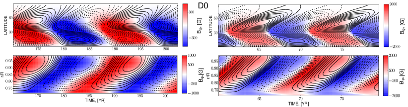
Figure 1: The time-latitude diagrams (top) for the radial magnetic field (contours) at the surface and the near-surface toroidal magnetic(image) field for the model D0 for the periods of rotation 25 (left) and 15 (right) days. The bottom line shows the same for the time-radius variation at $30^{\circ}$ latitude.

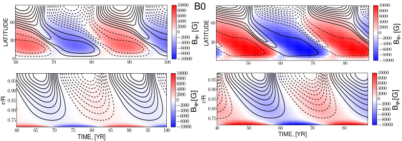
Figure 2: The same as Figure 1 for the model B0. The toroidal field in the time-latitude diagram is taken from the bottom of the convection zone.

3 Results

The study employs the same set of the basic parameters as in our previous paper (see, e.g. Pipin et al., 2013; Pipin & Kosovichev, 2014). Summary of the dynamo models is presented in the Table 1. The model parameters are chosen to reproduce the basic properties of the solar cycle, such as the cycle period of $\sim 11$ Yr, the magnitude of the polar field, $\sim 1$G, the total magnetic flux in the solar convection zone produced by the dynamo, $\sim 10^{24}$Mx, the time-latitude diagrams for the near-surface toroidal and radial magnetic fields (including the phase relation between them) as discussed in our previous papers (see, e.g, Pipin & Kosovichev 2014). For the B-type model we use parameters to make results for the solar case close to that discussed by Kitchatinov & Olemskoy (2011).

The numerical integration is carried out in latitude from pole to pole, and in radius from $r_{b}=0.715R_{\odot}$ to $r_{e}=0.99R_{\odot}$. The numerical scheme employs the pseudo-spectral approach for the numerical integration in latitude and the finite second-order differences in radius. The initial field was a weak dipole type poloidal magnetic field. The numerical scheme preserves the parity of the initial field unless there is a real parity braking process, e.g., associated with non-symmetric, relative to the equator, perturbations of the dynamo parameters. The initial conditions represent a weak dipole field with strength 0.01G.

For each rotation rate from the set $\left\{0.85,1,1.25,1.5,1.6,1.75\right\}\times\Omega_{0}$, where $\Omega_{0}=2.87\times 10^{-6}$s^-1 we study the different nonlinear dynamo regimes. The models D0 and B0 is related to the dynamo with the “algebraic” quenching of the $\alpha$-effect. The model D0 includes the buoyancy effect as well. In increasing the number of the model we include the other nonlinear effects, such as, the magnetic helicity and the magnetic feedback on the differential rotation, see details in the Table 2. The realistic model should include all those effects into account. The output of the models which we will use for comparison with observations includes, the total magnetic flux, which is integrated unsigned magnetic flux of the toroidal field over the bulk of the convection zone, the period of the magnetic cycle, the total Poynting flux from subsurface shear layer.

3.1 Spatial structure of dynamo waves

Figure 1 shows the time-latitude diagrams for the radial magnetic field at the surface and the near-surface toroidal magnetic field for the model D0, which takes into account the nonlinear $\alpha$- effect, and the magnetic buoyancy for the rotation periods of 25 and 15 days. Figure 2 shows the same as Figure 1 for the model B0. The butterfly diagrams of the model B0 for the period of rotation 25 days is rather similar to those by Kitchatinov & Olemskoy (2011). They noticed that in the model with the non-local $\alpha$-effect the dynamo wave does not follow to the Parker-Yoshimura rule. Thus, in their model the equatorward propagation of the dynamo wave is likely due to the joint action of the latitudinal shear and the strong diamagnetic pumping effect to the bottom of the convection zone.

The Figures 1,2 illustrate the main difference between the models with the “local” and non-local $\alpha$- effect. The radial propagation of the dynamo wave is outward for the D-type models and it is opposite for the B-type models. The downward propagation of the dynamo wave is a typical feature of the Babcock-Leighton types dynamo models (see, e.g., Dikpati & Charbonneau 1999). The downward propagation of the dynamo waves drives the magnetic field from the high latitudes at the top to the low latitudes at the bottom of the convection zone where the turbulent magnetic diffusivity is small. The amplitude of the turbulent diffusion is the key parameter that determines the period of the dynamo cycle. The increase of the rotation rate amplifies the concentration of the dynamo wave to the bottom of the convection zone. This likely results to increase of the dynamo period. Also, in the given examples of the B-type models, the maxims of the polar magnetic field corresponds to the maxims of the toroidal field at the low latitudes (cf, with the D-type models).

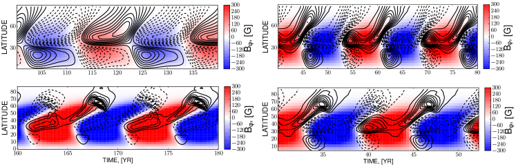
Figure 3: The time-latitude diagrams for the radial magnetic field (contours) at the surface and the near-surface toroidal magnetic(image) field for the model D1 for the set of the periods of rotation 25.3, 20.3,16.9 and 14.5 days clockwise starting from the up left.

The nonlinear effects due to magnetic buoyancy, magnetic helicity conservation results to saturation both the D-type and B-type dynamo models. Recently, Brandenburg et al. (2014) re-considered this effect for the two different kinds of the dynamical quenching in the B-type models. Here we confirm their results for the axisymmetric spherical dynamo models. Results in the Table 1 (see the B1) shows that the magnetic buoyancy quenches the magnetic flux produced by the dynamo by factor 2 (for the rotation period 25 days) to factor 4 (for the rotation period of 15 days). The magnetic buoyancy is less essential for the D-type models (Kichatinov & Pipin, 1993).

Quenching of the dynamo by the magnetic helicity conservation make a little change to the structure of the butterfly diagram of the B-type model. The changes in the D-type models are considerable. They are illustrated in the Figure 3. We find that the polar branch of the toroidal magnetic field becomes more and more pronounced when the period of the rotation is decreased. Also the character of the polar reversals is eventually changed from the smooth and monotonic kind as in the case of the 25-days period to the serge like pattern when the period of rotation is 14.5 days.

Figure 4: Top line: left panel shows the isolines of the mean distribution of the angular velocity in the star in the range $[0.63-0.98]\times$$\Omega\left(r,\theta\right)/\Omega_{\boldsymbol{\star}}$ ($\Omega_{\boldsymbol{\star}}$ - rotation rate of a star) with particular levels at 0.78,0.88 and 0.98 for the periods of rotation 25.3(blue color) and 14.5 days (red color), black color shows the unperturbed distribution; middle panel shows snapshots of the magnetic field distribution (contours) and the torsional oscillation (color image) for the model D2 with the period of rotation 25.3 days; the right panel shows the same as the middle panel for the period of rotation 14.5 days. The bottom line shows the same as the top line for the model B3.

3.2 Magnetic feedback on the differential rotation

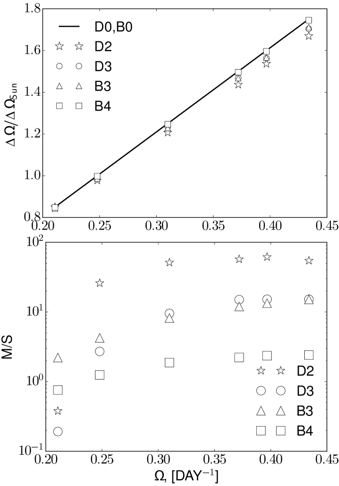
Figure 5: Top panel shows the mean surface differential rotation at the stationary state of the magnetic activity evolution, the black line shows the kinematic case. The bottom panel shows the maximum amplitude of the zonal velocity perturbation at latitude of 30^∘ north on the surface for the models D2, D3, B3 and B4.

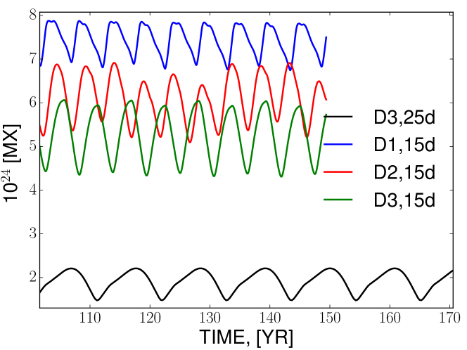
Figure 6: Variation of the total flux in D-type models

The further quenching of the dynamo process can be seen when we take into account the back reaction of the large-scale magnetic field on the angular momentum transport. It is found that the D- and B-type dynamo models produce the different effect on the angular momentum transport inside the convection zone. In the B-type model the torsional oscillations are concentrated to the bottom of the dynamo domain. Note that the situation can be different for the B-type model with regards for the meridional circulation and the magnetic backreaction on the heat transport (see, Rempel 2006).

Figure 4 shows the snapshots of the torsional oscillations and the mean states of the angular velocity distributions for the periods of rotation of 25.3 and 14.5 days for the D2 and B3 models. The torsional oscillations are determined as the difference between the instantaneous and the mean profiles of the angular velocity for the stationary stage of the magnetic activity evolution. The D2 and B3 models show the stronger deviation of the rotation profiles from the unperturbed state than the models D3 and B4. The magnetic helicity conservation quenches the amplitude of the torsional oscillations by means of damping the magnitude of the dynamo generated magnetic fields. For the D2 and B3 type models the distribution of the angular velocity deviates strongly from the radial-like profiles for the star rotating with the period of 14.5 days (see, e.g., Figure 4 (top,left). In the model D2 and B3 the rotation profiles in the mid part of the convection zone becomes more and more cylinder-like when the period of the rotation decreases.Figure 5 shows results for the surface differential rotation and the magnitude of the torsional oscillations in the dynamo modes D2, D3, B3 and B4. The magnitude of the torsional oscillations is determined by the maximum amplitude of the zonal velocity perturbation at latitude of 30^∘ north on the surface in the stationary state of evolution.

We find that in the model D2 the magnetic activity reduces the latitudinal shear at the surface by 10% of the $\Delta\Omega_{\odot}$, and the reduction is about 5% for the fully nonlinear dynamo model D3. In the B-type models the reduction of the latitudinal shear is about 5 % of the $\Delta\Omega_{\odot}$ in the case B3. In the fully nonlinear B-type dynamo model the change of the latitudinal shear is relatively small. It is less than 1 % of the $\Delta\Omega_{\odot}$. The magnitude of the torsional oscillations behave similarly. The model D2 with the period of rotation 14.5 days shows the torsional oscillations of magnitude about 70 m/s at the surface.

3.3 Dynamo amplitude and period vs period of rotation

We find that for the fast rotation case the nonlinear dynamos of D-type can show the multiply periods. However, in the given range of the rotational periods and for the given choice of the dynamo parameters, the regime of the multiply dynamo periods is not well developed. Figure 6 illustrates variations of the total unsigned magnetic flux of the toroidal field generated by the dynamo in the model D3 for the rotational periods 25.3 and 14.5 days and for the models D1 and D2 for the rotational period 14.5 days. For the period of rotation 14.5 days the D1 model for the shows the <<long-term>> variations with period about 5-6 of the basic periods. The long-term variations are damped by the nonlinear $\Lambda$- quenching effects and the large-scale Lorentz forces. It seems that the model D3 (with the rotational period 14.5 days) is near the threshold of the nonlinear regime with the <<long-term>> variations. This question should be studied further.

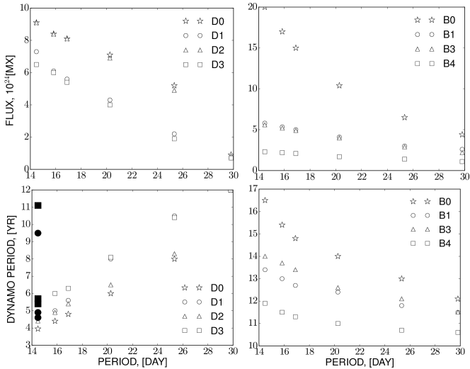
Figure 7: The top line show the dependence of the total magnetic flux generated by the dynamo versus the period of rotation. The bottom line shows the variations of the dynamo period. The filled symbols shows results for the models D1 and D3 with the multiply periods. In those cases, the results for the sum of the principal periods are shown as well.

Figure 7 illustrates our findings about dependence of the magnetic cycles parameters, such as the magnitude of the total magnetic flux and the dynamo period, on the period of rotation of the star. The models D1 and D3 have the weaker dynamo than the models D0 and D2. The model with the non-local $\alpha$ effect, the B0, has the strongest toroidal field for the set of our dynamo models. Surprisingly, that the amplitude of the toroidal magnetic flux in the models B1 and B3 is rather similar to the models D1 and D3. This tells us that the magnetic buoyancy quenches the B-types dynamo models in a more efficient way than for the D-type. Also, the total magnetic flux in the fully nonlinear B-type model is about factor 3 smaller than in the D-type.

The D-type models shows the decrease of the dynamo period with the decrease of the rotational period of the star. The period of magnetic cycles changes from about 11 years for the solar case to the value which is about 3 year for the star rotating with the period about 15 days. The opposite tendency is found for the B-types dynamo models, where the dynamo period increases from 11 to 17 years when the rotational period decreases.

The Table 2 gives results for the mean Poynting magnetic energy flux from the subsurface shear layer, $S_{M}$, for the D-type models. In the model we use the special boundary conditions, the Eq.(5) which allow the penetration of the toroidal field to the surface. In the linear case, this condition gives $S_{M}\sim B_{s}^{2}$, where $B_{s}$ is the toroidal magnetic field strength in the near-surface layer. In simulations it is found that the increase of the $S_{M}$ is gradually slow down when the rotation rates increase. Thus we can conclude that in the nonlinear dynamo the generated Poynting flux increases as $S_{M}\sim B_{s}^{2-\delta}$ where the $0<\delta<1$. This was predicted by Kleeorin et al. (1995) (cf., to Blackman & Thomas 2015) for the dynamo models with magnetic helicity conservation as the principal dynamo non-linearity. It is confirmed by Vidotto et al. (2014) who found $\delta\approx 1.61$ for the X-ray flux for magnetic activity in solar type stars. The flux reaches the magnitude $10^{-3}F_{\odot}$, where $F_{\odot}={\displaystyle\frac{L_{\odot}}{4\pi R_{\odot}^{2}}}$. The result is in the agreement with the observational findings (Katsova & Livshits, 2006). We postpone the detailed study of the Poynting flux in the nonlinear dynamo for the future.

In our calculations we compute the averaged surface magnetic field, as well. The results for this proxy of the stellar magnetic activity were published recently by Vidotto et al. (2014). For the given range of the rotation rates both the D- and B-types of the dynamo models reproduce the observational finding reasonably well. We postpone a more detailed comparison of these results with observations for a future.

It is noteworthy that the feedback of the magnetic helicity quenching on the large-scale dynamo depends on amount of the magnetic helicity in the dynamo region. This is partly controlled by the effective magnetic Reynolds number, $R_{m}$. The decrease of the $R_{m}$ simulates the increase of the helicity loss. It is found that for the $R_{m}=10^{2}$ the model D3 produces nearly the same amount of the total magnetic flux as the model D2. The similar effect can be expected for the B-type models. The increase of the turbulent diffusivity of the magnetic helicity will produce the similar effects as the decrease of the $R_{m}$ (see Hubbard & Brandenburg, 2012). It is likely that the helicity loss is modulated by the magnetic activity, e.g., by modulation of the coronal activity. Thus, the realistic dynamo model have to capture the basic mechanisms of the magnetic helicity loss, e.g., by means of including the stellar corona in simulations (see, Blackman & Brandenburg, 2003; Warnecke et al., 2011).

The D-type model was calibrated against the solar case. The eigenvalue analysis for the D-type models (see, Pipin 2012, and references therein) shows that variations of the free parameters, like the $C_{\delta}$ (the $\Omega\times J$ effect), the $C_{v}$ (stratification of the turbulent diffusivity) can produce a dynamo with steady and non-oscillating large-scale magnetic field. The changes from the oscillating to steady dynamo regimes with the increase of the rotation rates could happen in the D-type dynamo models for the range of the parameters $C_{\delta,v}$ different than we use in the paper. The nonlinear dynamo models in these cases should be studied separately.

4 Discussion and conclusions

In the paper we have studied the nonlinear effects in the large-scale magnetic solar-type dynamo on the parameters of the dynamo cycles for the range of the rotation periods from 14.5 to 30 days. This a preliminary study. The dynamo model lacks the self-consistent description of the angular momentum in the convection zone of a star. We also exclude the evolutionary changes of the stellar convection zone structure, which could occur together with the angular momentum loss. The model also lacks the effects of the meridional circulation to the dynamo action, which is found in the direct numerical simulations (Miesch et al., 2011; Guerrero et al., 2013a; Käpylä et al., 2014) and it is extensively used in the advection B-type solar dynamo models (Brun et al., 2014). Therefore I consider the results of the paper as preliminary.

We find that the D-type dynamo models (the dynamo distributed over the convection zone) satisfactory explains the dependence of the dynamo magnitude and the dynamo periods on the periods of rotation of the star (see, e.g., Soon et al. 1994; Saar 2011). These properties are expected from the qualitative predictions made for linear and weakly-nonlinear Parker-type dynamo models (Kuzanyan, 1998). For the Sun, the relation between the magnitude of the solar cycle and its period is a part of the Waldmeier’s relations (Waldmeier, 1936). The B-type models fails to explain the latter fact. In mean-field models of the stellar dynamo it was seen earlier by Jouve et al. (2010) and Karak et al. (2014). Here we confirm this effect on the B-type model without meridional circulation. Note, that the increase of the dynamo period with increase of magnitude of dynamo generated magnetic field was reported earlier by Ruediger & Brandenburg (1995) for the dynamo model in the overshoot layer below the convection zone. In their case the dynamo wave propagate inward to the bottom of the overshoot layer, see Fig.4 (right) in (Ruediger & Brandenburg, 1995). The similar is found in our study for the B-type model. This proves the generic character of this effect for this type of the large-scale dynamo. Figure 2 shows that in the B-type models the dynamo wave propagates to the bottom of the convection zone. Which is promoted by the diamagnetic pumping. The effect can be amplified in the model with the meridional circulation. The concentration of the dynamo wave to the bottom of the convection zone, where the magnetic diffusivity is low, is amplified for the fast rotating star. This enlarges the amplitude of the dynamo and the dynamo period as well. The certain set of the multiply meridional circulation cells can help to solve this issue (Jouve et al., 2010). However, it is not clear if such a set of the meridional circulation cells is consistent with the angular momentum transport.

It is found that the magnetic helicity conservation is the most efficient mechanism for the nonlinear quenching of the large-scale dynamo. We confirm the results about magnetic helicity quenching of the B-type dynamos which were reported earlier by Brandenburg & Käpylä (2007) and Brandenburg et al. (2014). Results for the given range of the rotational periods does not give enough confidence to conclude if there is a saturation level is reached in the B-type dynamos at the rotation period 15 days. An increase of the generated magnetic flux with the increase of the rotation rate remains constant for the all D-type dynamos. It is noteworthy, that the model of the magnetic helicity loss should be elaborated further for a better confidence in comparing the results of the mean-field dynamo models with observations.

The large-scale Lorentz force and the $\Lambda$- quenching reduce the surface differential rotation and produce the torsional oscillations. The effects are stronger in the D-type dynamo models than in the B-type models. This seems due to the distributed character of the magnetic feedback on the angular momentum balance for the dynamo operating in the whole convection zone. It is found that the magnetic backreaction on the surface differential rotation can be about 10 % of the solar value. Thus in the given interval of the rotational period the magnetic saturation of the differential rotation by the dynamo (see, e.g., Saar 2011) is not significant. Following to hints from observations it could be found for the higher rotation rates.

Analysis of observations of stellar magnetic activity (see, e.g., Soon et al. 1993; Baliunas et al. 1995; Saar & Brandenburg 1999; Böhm-Vitense 2007) reports the multiply branch of the dynamo activity for the cool stars. Results show the multiply periods on the Sun’s analog rotating with period about 15 days. The regime with multiply periods was reported in the solar-type dynamo models when the nonlinear system passes from the regular to chaotic behaviour (see, e.g., Brandenburg et al., 1989; Covas et al., 1998; Tobias, 1996; Pipin, 1999). In our set of the D-type models, the most realistic are the D2 and D3. Variation of the rotation rate in those models gives the different distribution of the periods. In reality, the magnetic helicity loss (see the end of subsection 3) we would give the mix of the distributions which are produced by the models D2 and D3. Therefore the given results do not show the distinct multiply branch of the dynamo activity. This interesting question will be addressed in the future studies.

I summarize the main results as follows. The nonlinear distributed mean-field solar dynamo model is calibrated versus the solar case. It has the basic properties of the solar cycle such as the cycle period, $\sim 11$Yr, the total magnetic flux produced in the dynamo, $\sim 10^{24}$Mx and the time-latitude diagrams for the large-scale magnetic field, in a good agreement with observation. The same model satisfactory reproduces the main properties of the stellar magnetic cycles on the Sun’s analogs for the range of rotational periods of 15-30 days.

Acknowledgements

The work is supported by RFBR under grants 14-02-90424, 15-02-01407 and the project II.16.3.1 of ISTP SB RAS. I’m grateful to anonymous referee for comments and suggestions. I also thank D. Moss, A.G. Kosovichev and K.M. Kuzanyan for a critical reading of the manuscript and helpful comments.

5 Appendix A

5.1 The $\boldsymbol{\mathcal{E}}$

This section of Appendix describes the parts of the mean-electromotive force which contribute in the Eq.(2).

5.1.1 The anisotropic diffusion

The anisotropic diffusion tensor $\eta_{ijk}$ was derived in (Pipin, 2008) (hereafter P08) and (Pipin & Kosovichev, 2014). The $\eta_{ijk}$ takes into account the generation of the magnetic fields by the $\Omega\times J$ effect (Rädler, 1969), as well. The $\eta_{ijk}$ reads

$$\eta_{ijk} = 3\eta_{T}\bigg{\{}\left(2f_{1}^{(a)}-f_{2}^{(d)}\right)\varepsilon_{ijk}+2f_{1}^{(a)}e_{i}e_{n}\varepsilon_{jnk}$$

$$+ \frac{a}{3}\phi_{1}\left(g_{n}g_{j}\varepsilon_{ink}-\varepsilon_{ijk}\right)\bigg{\}}$$

$$+ 3\eta_{T}C_{\delta}f_{4}^{(d)}e_{j}\left\{\tilde{\varphi}_{7}^{(w)}\delta_{ik}+\tilde{\varphi}_{2}^{(w)}\frac{\overline{B}_{i}\overline{B}_{k}}{\overline{B}^{2}}\right\},$$

where $\mathbf{e}={\displaystyle\boldsymbol{\Omega}/\Omega}$ is the unit vector along the rotation axis and $\mathbf{g}$ is the unit vector in the radial direction, $a$ is the parameter of the turbulence anisotropy, $\eta_{T}$ is the magnetic diffusion coefficient. The components of the $\eta_{ijk}$ depend on the Coriolis number $\Omega^{*}=4\pi{\displaystyle\frac{\tau_{c}}{P_{rot}}}$, where $P_{rot}$ is the rotational period, $\tau_{c}$ is the convective turnover time. The quenching functions $f_{1,2}^{(a,d)}$ and $\phi_{1}$ are

$$f_{1}^{(a)} = \frac{1}{4\Omega^{*\,2}}\left(\left(\Omega^{*\,2}+3\right)\frac{\arctan\Omega^{*}}{\Omega^{*}}-3\right),$$

$$f_{2}^{(d)} = \frac{1}{\Omega^{*\,2}}\left(\frac{\arctan\Omega^{*}}{\Omega^{*}}-1\right),$$

$$\phi_{1}\!\! = \!\!-\frac{1}{24\Omega^{\star 2}}\left(2\log\left(1+4\Omega^{\star 2}\right)+4\log\left(1+\Omega^{\star 2}\right)\right.$$

$$+ \left.\left(1-4\Omega^{\star 2}\right)\frac{\arctan\left(2\Omega^{\star}\right)}{\Omega^{\star}}\right.$$

$$+ \left.4\left(1-\Omega^{\star 2}\right)\frac{\arctan\left(\Omega^{\star}\right)}{\Omega^{\star}}-6\right).$$

The last term in the Eq.(5.1.1) is a contribution of the $\Omega\times J$ effect with a free parameter $C_{\delta}$ and the quenching functions of the magnetic field and the Coriolis number,$\tilde{\varphi}_{2,7}^{(w)}\left(\beta\right)$ and $f_{4}^{(d)}\left(\Omega^{*}\right)$:

$$\tilde{\varphi}_{2}^{(w)}\!\! \!=\! \!\!-\frac{5}{192\beta^{5}}\left(\!3\left(16\beta^{4}\!-\!5\right)\frac{\arctan\left(2\beta\right)}{2\beta}-5\left(4\beta^{2}-3\right)\right),$$

$$\tilde{\varphi}_{7}^{(w)} = \frac{5}{192\beta^{4}}\left(3\left(16\beta^{4}-1\right)\frac{\arctan\left(2\beta\right)}{2\beta}-\left(4\beta^{2}-3\right)\right),$$

$$f_{4}^{(d)} = \frac{1}{6\Omega^{*\,3}}\left(\left(2\Omega^{*\,2}+3\right)-3\left(\Omega^{*\,2}+1\right)\frac{\arctan\left(\Omega^{*}\right)}{\Omega^{*}}\right).$$

Note in the notation of P08 $\tilde{\varphi}_{2,7}^{(w)}\left(\beta\right)=\frac{5}{2}\varphi_{2,7}^{(w)}\left(\beta\right)$ and $\beta={\displaystyle\frac{\left|\overline{B}\right|}{\sqrt{4\pi\overline{\rho}u^{\prime 2}}}}$.

5.1.2 The $\alpha$-effect

The $\alpha$ effect takes into account the kinetic and magnetic helicities,

$$\alpha_{ij} = C_{\alpha}\sin^{2}\theta\psi_{\alpha}(\beta)\alpha_{ij}^{(H)}\eta_{T}+\alpha_{ij}^{(M)}\frac{\overline{\chi}\tau_{c}}{4\pi\overline{\rho}\ell^{2}}$$ (A2)

where $C_{\alpha}$ is a free parameter, the $\alpha_{ij}^{(H)}$ and $\alpha_{ij}^{(M)}$ represent the kinetic and magnetic helicity parts of the $\alpha$-effects, respectively, $\overline{\chi}$- is the small-scale magnetic helicity, the $\ell$ is the typical length scale of the turbulence, and $\bar{\rho}$ is the mean density. The $\alpha_{ij}^{(H)}$ reads,

$$\alpha_{ij}^{(H)} = \delta_{ij}\left\{3\left(f_{10}^{(a)}\left(\mathbf{e}\cdot\boldsymbol{\Lambda}^{(\rho)}\right)+f_{11}^{(a)}\left(\mathbf{e}\cdot\boldsymbol{\Lambda}^{(\eta)}\right)\right)\right\}$$

$$+ e_{i}e_{j}\left\{3\left(f_{5}^{(a)}\left(\mathbf{e}\cdot\boldsymbol{\Lambda}^{(\rho)}\right)+f_{4}^{(a)}\left(\mathbf{e}\cdot\boldsymbol{\Lambda}^{(\eta)}\right)\right)\right\}$$

$$+ 3\Bigl{\{}\left(e_{i}\Lambda_{j}^{(\rho)}+e_{j}\Lambda_{i}^{(\rho)}\right)f_{6}^{(a)}$$

$$+ \left(e_{i}\Lambda_{j}^{(\eta)}+e_{j}\Lambda_{i}^{(\eta)}\right)f_{8}^{(a)}\Bigr{\}}.$$

where $\mathbf{\boldsymbol{\Lambda}}_{i}^{(\rho)}=\boldsymbol{\nabla}_{i}\log\overline{\rho}$ are components of the gradient of the mean density, the $\mathbf{\boldsymbol{\Lambda}}^{(\eta)}=C_{v}\boldsymbol{\nabla}\log\left(\eta_{T}\right)$ is the same for the turbulent diffusivity. The free parameter $C_{v}$ influences the distribution of the kinetic $\alpha$-effect near the bottom of the convection zone and the strength of the diamagnetic pumping there (see below). The $\alpha_{ij}^{(M)}$ reads:

$$\alpha_{ij}^{(M)}=2f_{2}^{(a)}\delta_{ij}-2f_{1}^{(a)}e_{i}e_{j},$$ (A4)

The helicity density of the fluctuating part of magnetic field, $\overline{\chi}=\overline{\mathbf{a}\cdot\mathbf{b}}$, is governed by the conservation law:

$$\frac{\partial\overline{\chi}^{(tot)}}{\partial t}=-\frac{\overline{\chi}}{R_{m}\tau_{c}}-2\eta\overline{\mathbf{B}}\cdot\mathbf{\overline{J}}-\boldsymbol{\nabla\cdot}\boldsymbol{\boldsymbol{\mathcal{F}}}^{\chi},$$ (A5)

where $\overline{\chi}^{(tot)}=\overline{\chi}+\overline{\mathbf{A}}\cdot\overline{\mathbf{B}}$ is the total magnetic helicity density and the $\boldsymbol{\boldsymbol{\mathcal{F}}}^{\chi}=-\eta_{\chi}\boldsymbol{\nabla}\overline{\chi}$ is the diffusive flux of the magnetic helicity, with the $\eta_{\chi}=\frac{3}{10}\left(2f_{1}^{(a)}-f_{2}^{(d)}\right)\eta_{T}$, $f_{1,2}^{(a)}$ are the functions of the Coriolis number, $R_{m}$ is the magnetic Reynolds number. The $\eta_{\chi}$ is factor ten smaller than the isotropic part of the magnetic diffusivity (Mitra et al., 2010).

The quenching functions which define dependence of the $\alpha$-effect on the Coriolis number are

$$f_{2}^{(a)} = \frac{1}{4\Omega^{*\,2}}\left(\left(\Omega^{*\,2}+1\right)\frac{\arctan\Omega^{*}}{\Omega^{*}}-1\right),$$

$$f_{3}^{(a)} = \frac{1}{4\Omega^{*\,2}}\left(2-2\frac{\arctan\Omega^{*}}{\Omega^{*}}\right),$$

$$f_{4}^{(a)} = \frac{1}{6\Omega^{*\,3}}\Bigl{(}3\left(\Omega^{*4}+6\Omega^{*2}+5\right)\frac{\arctan\Omega^{*}}{\Omega^{*}}$$

$$- \left(13\Omega^{*2}+15\right)\Bigr{)},$$

$$f_{5}^{(a)} = \frac{1}{\Omega^{*}}\left(\left(\Omega^{*2}+3\right)\frac{\arctan\Omega^{*}}{\Omega^{*}}-3\right),$$

$$f_{6}^{(a)} = \frac{1}{6\Omega^{*\,3}}\left(3\left(\Omega^{*2}+2\right)\frac{\arctan\Omega^{*}}{\Omega^{*}}-\left(\Omega^{*2}+6\right)\right),$$

$$f_{8}^{(a)} = -\frac{1}{12\Omega^{*\,3}}\left(3\left(4\Omega^{*2}+2\right)\frac{\arctan\Omega^{*}}{\Omega^{*}}\right.$$

$$- \left.\left(10\Omega^{*2}+6\right)\right),$$

$$f_{10}^{(a)} = \frac{1}{\Omega^{*}}\left(1-\left(\Omega^{*2}+1\right)\frac{\arctan\Omega^{*}}{\Omega^{*}}\right),$$

$$f_{11}^{(a)} = -\frac{1}{6\Omega^{*\,3}}\left(3\left(\Omega^{*2}+1\right)^{2}\frac{\arctan\Omega^{*}}{\Omega^{*}}-\left(5\Omega^{*2}+3\right)\right),$$

Functions $f^{(a)}_{2-11}$ were defined in P08 for the general case which includes the effects the hydrodynamic and magnetic fluctuations in the background turbulence. Here, we write the expressions for the case when the background turbulent fluctuations of the small-scale magnetic field are in equipartition with the hydrodynamic fluctuations, i.e., ${\displaystyle\varepsilon=\frac{b^{\prime 2}}{4\pi\overline{\rho}u^{\prime 2}}}=1$, where the $u^{\prime 2}$ and $b^{\prime 2}$ are intensity of the background turbulent velocity and magnetic field. The magnetic quenching function of the hydrodynamic part of $\alpha$-effect is as follows

$$\psi_{\alpha}=\frac{5}{128\beta^{4}}\left(16\beta^{2}-3-3\left(4\beta^{2}-1\right)\frac{\arctan\left(2\beta\right)}{2\beta}\right).$$

Note in the notation of P08 $\psi_{\alpha}=-3/4\phi_{6}^{(a)}$.

5.1.3 The turbulent pumping

The turbulent pumping of the mean-field is the sum of the contributions due to the mean density gradient (Kichatinov, 1991), $\gamma_{ij}^{(\rho)}$, the diamagnetic pumping (Krivodubskij, 1987), $\gamma_{ij}^{(\eta)}$, the mean-field magnetic buoyancy (Kichatinov & Pipin, 1993), $\gamma_{ij}^{(b)}$, and effects due to the large-scale shear (Rogachevskii et al., 2011), $\gamma_{ij}^{(H)}$:

$$\gamma_{ij}=\gamma_{ij}^{(\rho)}+\gamma_{ij}^{(\eta)}+\gamma_{ij}^{(b)}+\gamma_{ij}^{(H)},$$ (A6)

where each contribution is defined as follows:

$$\gamma_{ij}^{(\rho)} = 3\eta_{T}\left\{f_{3}^{(a)}\Lambda_{n}^{(\rho)}+f_{1}^{(a)}\left(\mathbf{e}\cdot\boldsymbol{\Lambda}^{(\rho)}\right)e_{n}\right\}\varepsilon_{inj}$$

$$-3\eta_{T}f_{1}^{(a)}e_{j}\varepsilon_{inm}e_{n}\Lambda_{m}^{(\rho)}$$

$$\gamma_{ij}^{(\eta)} = \!\!\frac{3}{2}\eta_{T}\left\{f_{2}^{(a)}\Lambda_{n}^{(\eta)}\varepsilon_{inj}\!\!+\!\!f_{1}^{(a)}e_{j}\varepsilon_{inm}e_{n}\Lambda_{m}^{(\eta)}\varepsilon_{inm}\right\}$$ (A8)

$$\gamma_{ij}^{(b)} = \frac{\alpha_{MLT}u^{\prime}}{\gamma}\beta^{2}K\left(\beta\right)g_{n}\varepsilon_{inj},$$ (A9)

$$\gamma_{ij}^{(H)} = \left(f_{2}^{(\gamma)}\frac{\overline{\chi}}{\overline{\rho}\ell^{2}}+f_{1}^{(\gamma)}h_{\mathcal{K}}\right)\tau_{c}^{2}\varepsilon_{ikj}\overline{W}_{k}$$ (A10)

where $f_{1,2,3}^{(a)}\left(\Omega^{\star}\right)$ and $f_{1,2}^{(\gamma)}\left(\Omega^{\star}\right)$ - are functions of the Coriolis number, $u^{\prime}$ is the RMS of the convective velocity, the $\alpha_{MLT}=2$ is the parameter of the mixing length theory (the model by Stix 2002), $\gamma=5/3$ is the adiabatic exponent, $\mathbf{g}$ is the unit vector in the radial direction. The quenching of the magnetic buoyancy (see (Kichatinov & Pipin, 1993)) is determined by

$$K=\frac{1}{16\beta^{4}}\left(\frac{\left(\beta^{2}-3\right)}{\beta}\arctan\left(\beta\right)+\frac{\left(\beta^{2}+3\right)}{\left(\beta^{2}+1\right)}\right).$$

fIt is noteworthy that the mean-field magnetic buoyancy produces the mean drift of the horizontal magnetic field toward the surface. This reduces the efficiency of the dynamo process in the deep convection zone. The drift velocity is proportional to the pressure of the large-scale magnetic field. The $K(\beta)$ takes into account the feedback of the magnetic tensions on the buoyancy effect. For the magnetic field with strength of about the equipartition value, $\beta\sim 1$, the drift velocity is a few meters per second. The pumping effect $\gamma_{ij}^{(H)}$ is governed by the helicity parameters including the magnetic, $\overline{\chi}$, and kinetic helicity, $h_{\mathcal{K}}={\displaystyle\frac{3\eta_{T}}{2\tau_{c}}F_{1}\left(\Omega^{*}\right)\cos\theta\frac{\partial}{\partial r}}\log\left(\bar{\rho}u^{\prime}\right)$ (see, Kuzanyan et al. 2006), and the large-scale vorticity vector $\overline{\mathbf{W}}=\mathbf{\nabla}\times\overline{\mathbf{U}}$. Dependence of the $\gamma_{ij}^{(H)}$ on the Coriolis number is controlled by the quenching functions:

$$f_{1}^{(\gamma)} = \frac{1}{(24\Omega^{\ast})^{2}}\left(\left(1300\Omega^{\ast 2}+391\right)\frac{\arctan\left(2\Omega^{\ast}\right)}{2\Omega^{\ast}}\right.$$

$$- \left.1456\left(\Omega^{\ast 2}+1\right)\frac{\arctan\left(\Omega^{\ast}\right)}{\Omega^{\ast}}-3\left(32\Omega^{\ast 2}-355\right)\right),$$

$$F_{1} = \frac{1}{2\Omega^{*}}\left(\left(\Omega^{*2}-1\right)\frac{\arctan\Omega^{*}}{\Omega^{*}}+1\right)$$

and $f_{2}^{\left(\gamma\right)}=3f_{2}^{\left(a\right)}$. Pipin (2013) analyzed the total effect of the $\gamma_{ij}$ in details (see Fig.4 there). It was found that for the solar case, the $\gamma_{ij}$ results to the downward pumping in the most part of the convection zone. The velocity of the drift is a few meter per second in the main part of the convection zone. The magnitude of the latitudinal pumping of the toroidal magnetic field to equator is about 1 m/s.

5.2 The turbulent stresses

The turbulent stresses take into account the turbulent viscosity and generation of the large-scale shear due to the $\Lambda$- effect (Kitchatinov & Rüdiger, 1999):

$$T_{r\phi} = \overline{\rho}\nu_{T}\left\{\Phi_{\perp}+\left(\Phi_{\|}-\Phi_{\perp}\right)\mu^{2}\right\}r\frac{\partial\sin\theta\Omega}{\partial r}$$

$$+ \overline{\rho}\nu_{T}\sin\theta\left(\Phi_{\|}-\Phi_{\perp}\right)\left(1-\mu^{2}\right)\frac{\partial\Omega}{\partial\mu}$$

$$- \overline{\rho}\nu_{T}\sin\theta\Omega\left(\frac{\alpha_{MLT}}{\gamma}\right)^{2}\left(V^{(0)}+\sin^{2}\theta V^{(1)}\right),$$

$$T_{\theta\phi} = \overline{\rho}\nu_{T}\sin^{2}\theta\left\{\Phi_{\perp}+\left(\Phi_{\|}-\Phi_{\perp}\right)\sin^{2}\theta\right\}\frac{\partial\Omega}{\partial\mu}$$

$$+ \overline{\rho}\nu_{T}\left(\Phi_{\|}-\Phi_{\perp}\right)\mu\sin^{2}\theta r\frac{\partial\Omega}{\partial r}$$

$$+ \overline{\rho}\nu_{T}\mu\Omega\sin^{2}\theta\left(\frac{\alpha_{MLT}}{\gamma}\right)^{2}\left(H^{(0)}+\sin^{2}\theta H^{(1)}\right),$$

where $\mu=\cos\theta$, $\nu_{T}={\displaystyle\frac{4}{5}\eta_{T}}$. The viscosity functions - $\Phi_{\|},\Phi_{\perp}$ and the $\Lambda$- effect - $V^{\left(0,1\right)}$ and $H^{\left(0,1\right)}$, depend on the Coriolis number and the strength of the large-scale magnetic field. They also depend on the anisotropy of the convective flows. In following to Kitchatinov et al. (1999); Kitchatinov (2004) and Pipin (2004) we employ the following expressions:

$$\Phi_{\perp}\left(\Omega^{\star},\beta\right)\!\!\!\! \!=\! \!\!\psi_{\perp}\left(\Omega^{\star}\right)\left(\Phi_{q}\psi_{1}\left(\beta\right)\!+\!\left(1\!\!-\!\!\Phi_{q}\right)\phi_{V\perp}\left(\beta\right)\right),$$ (A13)

$$\Phi_{\parallel}\left(\Omega^{\star},\beta\right) = \psi_{\parallel}\left(\Omega^{\star}\right)\left(\Phi_{q}\psi_{1}\left(\beta\right)+\left(1-\Phi_{q}\right)\phi_{V}\left(\beta\right)\right),$$ (A14)

$$V^{(0)} = \left\{J_{0}\left(\Omega^{\star}\right)+J_{1}\left(\Omega^{\star}\right)+a\left(I_{0}\left(\Omega^{\star}\right)+I_{1}\left(\Omega^{\star}\right)\right)\right\}$$ (A15)

$$\times \left(\Phi_{q}K_{1}\left(\beta\right)+\left(1-\Phi_{q}\right)\phi_{V}\left(\beta\right)\right),$$

$$V^{(1)} = \left\{J_{1}\left(\Omega^{\star}\right)+aI_{1}\left(\Omega^{\star}\right)\right\}$$ (A16)

$$\times \left(\Phi_{q}K_{1}\left(\beta\right)+\left(1-\Phi_{q}\right)\phi_{V}\left(\beta\right)\right),$$

$$H^{(0)} = J_{4}\left(\Omega^{\star}\right)\phi_{H}\left(\beta\right),$$ (A17)

$$H^{(1)} = -V^{(1)},$$ (A18)

where, ${\displaystyle{\Phi_{q}=\frac{\arctan\Omega^{\star}}{\Omega^{\star}}}}$. We employ the quenching functions which were derived in the previous studies, e.g., the $\psi_{\perp,\parallel}$, $\psi_{1}$, $K_{1}$ and $J_{0,1}$ can be found in (Kueker et al., 1993; Kitchatinov et al., 1994; Kueker et al., 1996), the $I_{0,1}$ - in (Kitchatinov, 2004). For convenience we put them here,

$$\psi_{\parallel} = \frac{15}{32\Omega^{*4}}\Bigl{(}21-3\Omega^{*2}+\frac{4\Omega^{*2}}{1+\Omega^{*2}}$$

$$- \left(21+4\Omega^{*2}-\Omega^{*4}\right)\frac{\arctan\Omega^{*}}{\Omega^{*}}\Bigr{)},$$

$$\psi_{\perp} = \frac{15}{128\Omega^{*4}}\Bigl{(}\Omega^{*2}-21-\frac{8\Omega^{*2}}{1+\Omega^{*2}}$$ (A20)

$$+ \left(21+14\Omega^{*2}+\Omega^{*4}\right)\frac{\arctan\Omega^{*}}{\Omega^{*}}\Bigr{)}.$$ (A21)

$$J_{0} = \frac{1}{2\Omega^{*4}}\left(9-\frac{2\Omega^{*2}}{1+\Omega^{*2}}-\left(\Omega^{*2}+9\right)\frac{\arctan\Omega^{*}}{\Omega^{*}}\right),$$ (A22)

$$J_{1} = \frac{1}{2\Omega^{*4}}\Bigl{(}\frac{45+42\Omega^{*2}+\Omega^{*4}}{1+\Omega^{*2}}$$

$$+ \left(\Omega^{*4}-12\Omega^{*2}-459\right)\frac{\arctan\Omega^{*}}{\Omega^{*}}\Bigr{)},$$

$$I_{0} = -\frac{3}{4\Omega^{*4}}\left(\frac{3+\Omega^{*2}}{1+\Omega^{*2}}+\left(\Omega^{*2}-3\right)\frac{\arctan\Omega^{*}}{\Omega^{*}}\right),$$ (A24)

$$I_{1} = \frac{3}{4\Omega^{*4}}\Bigl{(}\frac{2\Omega^{*2}}{1+\Omega^{*2}}-15$$

$$+ \left(3\Omega^{*2}+15\right)\frac{\arctan\Omega^{*}}{\Omega^{*}}\Bigr{)},$$

$$K_{1} = \frac{1}{16\beta^{4}}\left(\frac{\beta^{2}+1}{\beta}\arctan\beta-1-\frac{2\beta^{2}}{3\left(1+\beta^{2}\right)}\right)$$ (A26)

The magnetic quenching functions $\phi_{H,V}$ follows from the general expression for the $\Lambda$ - effect and the turbulent viscosity for the fast rotating regime ($\Omega^{\star}>1$) given by Kueker et al. (1996) and by Pipin (2004). They are defined as follows:

$$\phi_{V\perp} = \frac{4}{\beta^{4}\sqrt{\left(1+\beta^{2}\right)^{3}}}\left(\left(\beta^{4}+19\beta^{2}+18\right)\sqrt{\left(1+\beta^{2}\right)}\right.$$ (A27)

$$- \left.8\beta^{4}-28\beta^{2}-18\right),$$

$$\phi_{V} = \frac{2}{\beta^{2}}\left(1-\frac{1}{\sqrt{\left(1+\beta^{2}\right)}}\right),$$ (A28)

$$\phi_{H} = \frac{4}{\beta^{2}}\left(\frac{2+3\beta^{2}}{2\sqrt{\left(1+\beta^{2}\right)^{3}}}-1\right).$$ (A29)

The Eqs.(A13-A30) take into account the different regimes of the magnetic quenching of the $\Lambda$-effect and the eddy viscosity in the cases of the slow ($\Omega^{\star}\ll 1$) and the fast rotation ($\Omega^{\star}\gg 1$). In particular, for the case $\Omega^{\star}\ll 1$ the turbulent viscosity is quenched as $\beta^{-1}$ when $\beta>1$ , and for the case $\Omega^{\star}\gg 1$ there is a stronger quenching, $\beta^{-2}$. Thus, in the presence of the strong large-scale toroidal magnetic field, the ratio between the eddy viscosity along and perpendicular to rotation axis is decreased (Pipin, 2004).

References

- Abramenko et al. (2011) Abramenko V. I., Carbone V., Yurchyshyn V., Goode P. R., Stein R. F., Lepreti F., Capparelli V., Vecchio A., 2011, ApJ, 743, 133
- Babcock (1961) Babcock H. W., 1961, ApJ, 133, 572
- Baliunas et al. (1995) Baliunas S. L., Donahue R. A., Soon W. H., Horne J. H., Frazer J., Woodard-Eklund L., Bradford M., Rao L. M., Wilson O. C., Zhang Q., Bennett W., Briggs J., Carroll S. M., Duncan D. K., Figueroa D., Lanning H. H., Misch T., Mueller J., Noyes R. W., Poppe D., Porter A. C., Robinson C. R., Russell J., Shelton J. C., Soyumer T., Vaughan A. H., Whitney J. H., 1995, ApJ, 438, 269
- Blackman & Brandenburg (2003) Blackman E. G., Brandenburg A., 2003, ApJL, 584, L99
- Blackman & Thomas (2015) Blackman E. G., Thomas J. H., 2015, MNRAS, 446, L51
- Böhm-Vitense (2007) Böhm-Vitense E., 2007, ApJ, 657, 486
- Brandenburg (2005) Brandenburg A., 2005, Astrophys. J., 625, 539
- Brandenburg et al. (2014) Brandenburg A., Hubbard A., Käpylä P. J., 2014, ArXiv e-prints
- Brandenburg & Käpylä (2007) Brandenburg A., Käpylä P. J., 2007, New Journal of Physics, 9, 305
- Brandenburg et al. (1989) Brandenburg A., Krause F., Meinel R., Moss D., Tuominen I., 1989, A & A, 213, 411
- Brandenburg & Sokoloff (2002) Brandenburg A., Sokoloff D., 2002, Geophys. Astrophys. Fluid Dyn., 96, 319
- Brandenburg & Subramanian (2005) Brandenburg A., Subramanian K., 2005, Phys. Rep., 417, 1
- Brun et al. (2014) Brun A., Garcia R., Houdek G., Nandy D., Pinsonneault M., 2014, Space Science Reviews, pp 1–54
- Brun et al. (2010) Brun A. S., Antia H. M., Chitre S. M., 2010, A & A, 510, A33+
- Charbonneau (2011) Charbonneau P., 2011, Living Reviews in Solar Physics, 2, 2
- Choudhuri et al. (1995) Choudhuri A. R., Schussler M., Dikpati M., 1995, A & A, 303, L29
- Covas et al. (2000) Covas E., Tavakol R., Moss D., Tworkowski A., 2000, A & A, 360, L21
- Covas et al. (1998) Covas E., Tavakol R., Tworkowski A., Brandenburg A., 1998, A & A, 329, 350
- Dikpati & Charbonneau (1999) Dikpati M., Charbonneau P., 1999, ApJ, 518, 508
- Donati & Landstreet (2009) Donati J.-F., Landstreet J. D., 2009, Ann. Rev. Astron and Astroph., 47, 333
- Folsom et al. (2014) Folsom C. P., Petit P., Bouvier J., Donati J.-F., Morin J., 2014, in IAU Symposium Vol. 302 of IAU Symposium, The evolution of surface magnetic fields in young solar-type stars. pp 110–111
- Guerrero et al. (2013a) Guerrero G., Smolarkiewicz P. K., Kosovichev A., Mansour N., 2013a, in Solar and Astrophysical Dynamos and Magnetic Activity, IAUS 294 Solar differential rotation: hints to reproduce a near-surface shear layer in global simulations
- Guerrero et al. (2013b) Guerrero G., Smolarkiewicz P. K., Kosovichev A. G., Mansour N. N., 2013b, ApJ, 779, 176
- Gunn et al. (1998) Gunn A. G., Mitrou C. K., Doyle J. G., 1998, MNRAS, 296, 150
- Hotta & Yokoyama (2011) Hotta H., Yokoyama T., 2011, ApJ, 740, 12
- Howe et al. (2011) Howe R., Larson T. P., Schou J., Hill F., Komm R., Christensen-Dalsgaard J., Thompson M. J., 2011, Journal of Physics Conference Series, 271, 012061
- Hubbard & Brandenburg (2012) Hubbard A., Brandenburg A., 2012, ApJ, 748, 51
- Jouve et al. (2010) Jouve L., Brown B. P., Brun A. S., 2010, A & A, 509, A32
- Käpylä et al. (2014) Käpylä P. J., Käpylä M. J., Brandenburg A., 2014, A & A, 570, A43
- Käpylä et al. (2006) Käpylä P. J., Korpi M. J., Tuominen I., 2006, Astronomische Nachrichten, 327, 884
- Karak et al. (2014) Karak B. B., Kitchatinov L. L., Choudhuri A. R., 2014, ApJ, 791, 59
- Katsova & Livshits (2006) Katsova M. M., Livshits M. A., 2006, Astronomy Reports, 50, 579
- Katsova et al. (2010) Katsova M. M., Livshits M. A., Soon W., Baliunas S. L., Sokoloff D. D., 2010, New Astr., 15, 274
- Katsova et al. (2013) Katsova M. M., Livshits M. A., Mishenina T. V., 2013, Geomagnetism and Aeronomy, 53, 937
- Kholikov et al. (2014) Kholikov S., Serebryanskiy A., Jackiewicz J., 2014, ApJ, 784, 145
- Kichatinov (1991) Kichatinov L. L., 1991, Astron. Astrophys., 243, 483
- Kichatinov & Pipin (1993) Kichatinov L. L., Pipin V. V., 1993, A & A, 274, 647
- Kim & Demarque (1996) Kim Y.-C., Demarque P., 1996, ApJ, 457, 340
- Kitchatinov (2004) Kitchatinov L. L., 2004, Astronomy Reports, 48, 153
- Kitchatinov (2013) Kitchatinov L. L., 2013, in Kosovichev A. G., de Gouveia Dal Pino E., Yan Y., eds, IAU Symposium Vol. 294 of IAU Symposium, Theory of differential rotation and meridional circulation. pp 399–410
- Kitchatinov & Olemskoy (2011) Kitchatinov L. L., Olemskoy S. V., 2011, Astronomy Letters, 37, 286
- Kitchatinov et al. (1999) Kitchatinov L. L., Pipin V. V., Makarov V. I., Tlatov A. G., 1999, Sol.Phys., 189, 227
- Kitchatinov et al. (1994) Kitchatinov L. L., Pipin V. V., Ruediger G., 1994, Astronomische Nachrichten, 315, 157
- Kitchatinov & Rüdiger (1999) Kitchatinov L. L., Rüdiger G., 1999, A & A, 344, 911
- Kleeorin & Rogachevskii (2003) Kleeorin N., Rogachevskii I., 2003, Phys. Rev. E, 67, 026321
- Kleeorin et al. (1995) Kleeorin N., Rogachevskii I., Ruzmaikin A., 1995, A & A, 297, 159
- Kleeorin & Ruzmaikin (1982) Kleeorin N. I., Ruzmaikin A. A., 1982, Magnetohydrodynamics, 18, 116
- Kosovichev et al. (2013) Kosovichev A. G., Pipin V. V., Zhao J., 2013, in Shibahashi H., Lynas-Gray A. E., eds, Progress in Physics of the Sun and Stars: A New Era in Helio- and Asteroseismology Vol. 479 of Astronomical Society of the Pacific Conference Series, Helioseismic Constraints and a Paradigm Shift in the Solar Dynamo. p. 395
- Krause & Rädler (1980) Krause F., Rädler K.-H., 1980, Mean-Field Magnetohydrodynamics and Dynamo Theory. Berlin: Akademie-Verlag
- Krivodubskij (1987) Krivodubskij V. N., 1987, Soviet Astronomy Letters, 13, 338
- Kueker et al. (1993) Kueker M., Ruediger G., Kitchatinov L. L., 1993, A & A, 279, L1
- Kueker et al. (1996) Kueker M., Ruediger G., Pipin V. V., 1996, A & A, 312, 615
- Kuzanyan (1998) Kuzanyan K. M., 1998, in Donahue R. A., Bookbinder J. A., eds, Cool Stars, Stellar Systems, and the Sun Vol. 154 of Astronomical Society of the Pacific Conference Series, Hale’s Polarity Law for Fast Rotating Stars from the Viewpoint of Dynamo Theory. p. 1286
- Kuzanyan et al. (2006) Kuzanyan K. M., Pipin V. V., Seehafer N., 2006, Sol.Phys., 233, 185
- Malkus & Proctor (1975) Malkus W. V. R., Proctor M. R. E., 1975, Journal of Fluid Mechanics, 67, 417
- Marsden et al. (2014) Marsden S. C., Petit P., Jeffers S. V., Morin J., Fares R., Reiners A., do Nascimento J.-D., Aurière M., Bouvier J., Carter B. D., Catala C., Dintrans B., Donati J.-F., Gastine T., Jardine M., Konstantinova-Antova R., Lanoux J., Lignières F., Morgenthaler A., Ramìrez-Vèlez J. C., Théado S., Van Grootel V., BCool Collaboration 2014, MNRAS, 444, 3517
- Miesch et al. (2011) Miesch M. S., Brown B. P., Browning M. K., Brun A. S., Toomre J., 2011, in Brummell N. H., Brun A. S., Miesch M. S., Ponty Y., eds, IAU Symposium Vol. 271 of IAU Symposium, Magnetic Cycles and Meridional Circulation in Global Models of Solar Convection. pp 261–269
- Miesch & Toomre (2009) Miesch M. S., Toomre J., 2009, Annual Review of Fluid Mechanics, 41, 317
- Mitra et al. (2010) Mitra D., Candelaresi S., Chatterjee P., Tavakol R., Brandenburg A., 2010, Astronomische Nachrichten, 331, 130
- Morin et al. (2013) Morin J., Jardine M., Reiners A., Shulyak D., Beeck B., Hallinan G., Hebb L., Hussain G., Jeffers S. V., Kochukhov O., Vidotto A., Walkowicz L., 2013, Astronomische Nachrichten, 334, 48
- Moss & Brandenburg (1992) Moss D., Brandenburg A., 1992, A & A, 256, 371
- Moss & Brooke (2000) Moss D., Brooke J., 2000, MNRAS, 315, 521
- Noyes et al. (1984) Noyes R. W., Weiss N. O., Vaughan A. H., 1984, ApJ, 287, 769
- Parker (1955) Parker E., 1955, Astrophys. J., 122, 293
- Pipin (1999) Pipin V. V., 1999, A & A, 346, 295
- Pipin (2004) Pipin V. V., 2004, PhD thesis, Institute solar-terrestrial physics, ( Dr Habil Thesis, in Russian)
- Pipin (2008) Pipin V. V., 2008, Geophysical and Astrophysical Fluid Dynamics, 102, 21
- Pipin (2013) Pipin V. V., 2013, Geophysical and Astrophysical Fluid Dynamics, 107, 185
- Pipin & Kosovichev (2011) Pipin V. V., Kosovichev A. G., 2011, ApJ, 741, 1
- Pipin & Kosovichev (2014) Pipin V. V., Kosovichev A. G., 2014, ApJ, 785, 49
- Pipin et al. (2012) Pipin V. V., Sokoloff D. D., Usoskin I. G., 2012, A & A, 542, A26
- Pipin et al. (2013) Pipin V. V., Zhang H., Sokoloff D. D., Kuzanyan K. M., Gao Y., 2013, MNRAS, 435, 2581
- Rädler (1969) Rädler K.-H., 1969, Monats. Dt. Akad. Wiss., 11, 194
- Reiners (2012) Reiners A., 2012, Living Reviews in Solar Physics, 9
- Rempel (2006) Rempel M., 2006, ApJ, 647, 662
- Rogachevskii et al. (2011) Rogachevskii I., Kleeorin N., Käpylä P. J., Brandenburg A., 2011, Phys. Rev. E, 84, 056314
- Rüdiger & Kichatinov (1993) Rüdiger G., Kichatinov L. L., 1993, Astron. Astrophys., 269, 581
- Ruediger (1989) Ruediger G., 1989, Differential rotation and stellar convection. Sun and the solar stars
- Ruediger & Brandenburg (1995) Ruediger G., Brandenburg A., 1995, A & A, 296, 557
- Saar (2011) Saar S. H., 2011, in Prasad Choudhary D., Strassmeier K. G., eds, IAU Symposium Vol. 273 of IAU Symposium, Starspots, cycles, and magnetic fields. pp 61–67
- Saar & Brandenburg (1999) Saar S. H., Brandenburg A., 1999, ApJ, 524, 295
- Soon et al. (1993) Soon W. H., Baliunas S. L., Zhang Q., 1993, ApJL, 414, L33
- Soon et al. (1994) Soon W. H., Baliunas S. L., Zhang Q., 1994, Sol.Phys., 154, 385
- Stix (2002) Stix M., 2002, The sun: an introduction, 2 edn. Berlin : Springer
- Tobias (1996) Tobias S. M., 1996, A & A, 307, L21
- Vidotto et al. (2014) Vidotto A. A., Gregory S. G., Jardine M., Donati J. F., Petit P., Morin J., Folsom C. P., Bouvier J., Cameron A. C., Hussain G., Marsden S., Waite I. A., Fares R., Jeffers S., do Nascimento J. D., 2014, MNRAS, 441, 2361
- Vitinsky et al. (1986) Vitinsky Y. I., Kopecky M., Kuklin G. V., 1986, The statistics of sunspots (Statistika pjatnoobrazovatelnoj dejatelnosti solntsa). Nauka, Moscow
- Waldmeier (1936) Waldmeier M., 1936, Astron. Nachrichr., 259, 267
- Warnecke et al. (2011) Warnecke J., Brandenburg A., Mitra D., 2011, A & A, 534, A11
- Yoshimura (1975) Yoshimura H., 1975, ApJ, 201, 740
- Zhao et al. (2013) Zhao J., Bogart R. S., Kosovichev A. G., Duvall Jr. T. L., Hartlep T., 2013, ApJL, 774, L29