Efficient scheme for generation of photonic NOON states in circuit QED

Abstract

We propose an efficient scheme for generating photonic NOON states of two resonators coupled to a four-level superconducting flux device. This proposal operates essentially by employing a technique of a coupler device resonantly interacting with two resonators simultaneously. As a consequence, the NOON-state preparation requires only $N+1$ operational steps and thus is much faster when compared with a recent proposal [Q. P. Su et al., Scientific Reports 4, 3898 (2014)] requiring $2N$ steps of operation. Moreover, due to the use of only two resonators and a device, the experimental setup is much simplified when compared with previous proposals requiring three resonators and two superconducting qubits/qutrits.

In recent years there is considerable interest in the entangled NOON states $\left|N0\right\rangle+\left|0N\right\rangle$, which have significant applications in quantum optical lithography [1], quantum metrology [2], precision measurement of transmons [3], and quantum information processing [4]. Based on circuit QED [5,6], several proposals have been presented to generate the photonic NOON states of two resonators [7-11].

The scheme in [7] requires that the pulse Rabi frequency is much smaller than the photon-number-dependent Stark shifts induced by dispersive interaction. Thus, the operation time needed to complete a rotation in each step is quite long. Another method was proposed [8] and implemented in experiment for $N\leq 3$ with a fidelity $0.33$ for $N=3$ [9]. This method shortens the operation time due to using resonant interaction but needs a complex setup (i.e., three resonators and two superconducting qutrits), which increases the experimental difficulty. Moreover, two classical pulses (e.g., a double pulse) are separately applied to the two qutrits during each step, conditional on the NOON state being prepared with $N$ steps. The scheme in [10] employs a complicated pulse. Similar to [8,9], this scheme requires two auxiliary superconducting qubits initially prepared in a Bell state. As argued there, to obtain a pure photonic NOON state, additional techniques are required to decouple the qubits from the resonators.

Recently, Q.P.Su et al. have proposed an alternative scheme for generating the NOON states of two resonators or cavities [11]. Compared with the previous proposals [8-10], the experimental setup is greatly simplified because of employing one superconducting qutrit and two resonators only. Due to using the resonant interaction, the operation can be performed much faster when compared with the method in [7]. However, as discussed in [11], $2N$ steps of operation are needed.

We here employ a four-level superconducting flux device to couple two resonators (hereafter the term cavity and resonator is used interchangeably). Different from the previous proposals [7-11], the device is simultaneously resonant with two cavities and thus two photons can be simultaneously created each in one cavity for each of the first $N-1$ operational steps.

This scheme only requires $N+1$ operational steps and thus the operation is much speeded up when compared with the recent proposal [11] requiring $2N$ steps. Numerical simulation shows that a high fidelity generation of the NOON state with $N\leq 10$ is feasible within present-day circuit QED. Further, this scheme has additional advantages: (i) Because of using only two resonators and a device, the setup is much simplified when compared with Refs. [8-10]; (ii) Due to using resonant interaction, the operation can be performed much faster when compared with [7]. Hence, the present scheme avoids most of the problems existing in the previous proposals.

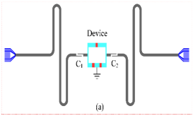
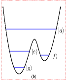
Figure 1: (color online). (a) Setup for two cavities and a superconducting flux device. Each cavity is a one-dimensional transmission line resonator. The device is connected to the two cavities via capacitors $c_{i}(i=1,2)$. (b) Four Levels of the device with a double potential well.

Consider two cavities coupled to a flux device with four levels $|g\rangle,~{}|e\rangle,~{}|f\rangle,~{}$and $|a\rangle$ (Fig. 1). Initially, the device is in the state $\frac{1}{\sqrt{2}}(\left|e\right\rangle+\left|a\right\rangle)$ and each cavity in a vacuum state $|0\rangle$. The device is initially decoupled from the two cavities, which can be achieved by a prior adjustment of the device level spacings. Note that for a flux device, the level spacings can be rapidly adjusted via varying external control parameters [12,13]).

Define $\omega_{eg},$ $\omega_{af},$ $\omega_{ae}$ as the $|g\rangle\leftrightarrow|e\rangle,$ $|f\rangle\leftrightarrow|a\rangle$ and $|e\rangle\leftrightarrow|a\rangle$ transition frequencies of the device, respectively. The frequency, initial phase, and duration of the pulse are denoted as {$\omega,$ $\varphi,$ $t$}.

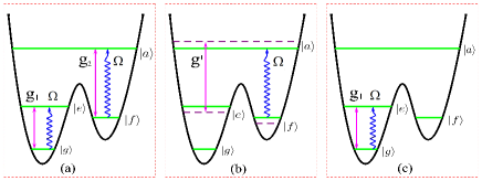
Figure 2: (color online). Illustration of resonant interaction between the device and the cavity/pulse during the NOON state preparation. Figures (a), (b) and (c) are for first $N-1$ steps, step $N$, and step $N+1$, respectively. In (b), dashed lines represent the adjusted energy levels.

To begin with, the level spacings of the device needs to be adjusted to have cavity $1$ ($2$) resonant with $\left|g\right\rangle\leftrightarrow\left|e\right\rangle$ ($\left|f\right\rangle\leftrightarrow\left|a\right\rangle$) transition [Fig. 2(a)]. The procedure for the NOON-state generation is described below:

Step $1$: Let cavity 1 (2) resonant with the $|g\rangle\leftrightarrow|e\rangle$ ($|f\rangle\leftrightarrow|a\rangle$) transition [Fig. 2 (a)]. In the interaction picture (the same picture is used without mentioning hereafter), the interaction Hamiltonian is $H_{1}=g_{1}(a_{1}\sigma_{eg}^{+}+h.c.)+g_{2}(a_{2}\sigma_{af}^{+}+h.c.),$ where $\sigma_{eg}^{+}=|e\rangle\langle g|$, $\sigma_{af}^{+}=|a\rangle\langle f|,$ $a_{1}$ ($a_{2}$) is the photon annihilation operator for cavity $1$ ($2$), and $g_{1}$ ($g_{2}$) is the coupling strength between cavity $1$ ($2$) and the $|g\rangle\leftrightarrow|e\rangle$ ($|f\rangle\leftrightarrow|a\rangle$) transition. Note that $g_{1}$ ($g_{2}$) depends on the coupling capacitance $c_{1}$ ($c_{2}$). Thus, set $g_{1}=g_{2}=g$, which can in principle be met by a prior design of the sample with appropriate $c_{1}$ and $c_{2}.$ Under $H_{1}$, the time evolution of the states $\left|e\right\rangle\left|n\right\rangle_{1}\left|0\right\rangle_{2}$ and $\left|a\right\rangle\left|0\right\rangle_{1}\left|n\right\rangle_{2}$ is described by

$$\left|e\right\rangle\left|n\right\rangle_{1}\left|0\right\rangle_{2} \rightarrow C\left|e\right\rangle\left|n\right\rangle_{1}\left|0\right\rangle_{2}-iD\left|g\right\rangle\left|n+1\right\rangle_{1}\left|0\right\rangle_{2},$$ (1)

$$\left|a\right\rangle\left|0\right\rangle_{1}\left|n\right\rangle_{2} \rightarrow C\left|a\right\rangle\left|0\right\rangle_{1}\left|n\right\rangle_{2}-iD\left|f\right\rangle\left|0\right\rangle_{1}\left|n+1\right\rangle_{2},$$ (2)

where $C=\cos(\sqrt{n+1}gt),$ $D=\sin(\sqrt{n+1}gt),$ subscripts $1$ ($2$) represents cavity 1 (2), $\left|n\right\rangle$ and $\left|n+1\right\rangle$ are the cavity photon-number states. For simplicity, define $|i\rangle_{1}|j\rangle_{2}=$ $|i\rangle|j\rangle$ with $i,j\in\{0,1,...,N\}$. Eqs. (1) and (2) show that after an interaction time $t_{1}=\frac{\pi}{2g}$(i.e., half a Rabi oscillation), the state $|e\rangle|0\rangle|0\rangle$ changes to $-i|g\rangle|1\rangle|0\rangle$ while the state $|a\rangle|0\rangle|0\rangle$ changes to $-i|f\rangle|0\rangle|1\rangle.$ Thus, the initial state $\frac{\sqrt{2}}{2}(|e\rangle+|a\rangle)|0\rangle|0\rangle$ of the system evolves to

$$\frac{-i}{\sqrt{2}}(|g\rangle|1\rangle|0\rangle+|f\rangle|0\rangle|1\rangle).$$ (3)

Now, apply a double pulse of $\{\omega_{eg},-\frac{\pi}{2},\frac{\pi}{2\Omega}\}$ and $\{\omega_{af},-\frac{\pi}{2},\frac{\pi}{2\Omega}\}$ to the device. The identical Rabi frequency $\Omega$ of each pulse can be achieved by adjusting the pulse intensities. The interaction Hamiltonian is given by $H_{2}=(\Omega e^{i\pi/2}\sigma_{eg}^{+}+h.c.)+(\Omega e^{i\pi/2}\sigma_{af}^{+}+h.c.),$ Under the Hamiltonian $H_{2}$, the time evolution of the states $\left|g\right\rangle,$ $\left|e\right\rangle,$ and $\left|f\right\rangle$ is described by

$$\left|g\right\rangle \rightarrow \cos\Omega t\left|g\right\rangle+\sin\Omega t\left|e\right\rangle,$$ (4)

$$\left|e\right\rangle \rightarrow -\sin\Omega t\left|g\right\rangle+\cos\Omega t\left|e\right\rangle,$$ (5)

$$\left|f\right\rangle \rightarrow \cos\Omega t\left|f\right\rangle+\sin\Omega t\left|a\right\rangle.$$ (6)

For $\Omega\gg g$, the interaction between cavities and the device can be neglected during the pulse. Based on Eqs. (4-6), the pulse leads to $|g\rangle\rightarrow\left|e\right\rangle$ and $|f\rangle\rightarrow|a\rangle.$ As a consequence, the state (3) becomes

$$\frac{-i}{\sqrt{2}}(|e\rangle|1\rangle|0\rangle+|a\rangle|0\rangle|1\rangle).$$ (7)

Step $j$ ($j=2,3,...,N-1$): Repeat the operation of step 1. The time for the device resonant with the two cavities is $t_{j}=\frac{\pi}{2\sqrt{j}g}$. Eqs. (1) and (2) show that after $t_{j},$ the state $|e\rangle|j-1\rangle|0\rangle$ changes to $-i|g\rangle|j\rangle|0\rangle$ and the state $|a\rangle|0\rangle|j-1\rangle$ becomes $-i|f\rangle|0\rangle|j\rangle$, which further turn into $-i|e\rangle|j\rangle|0\rangle$ and $-i|a\rangle|0\rangle|j\rangle$ respectively, due to a double pulse of $\{\omega_{eg},-\frac{\pi}{2},\frac{\pi}{2\Omega}\}$ and $\{\omega_{af},-\frac{\pi}{2},\frac{\pi}{2\Omega}\}$ pumping the state $\left|g\right\rangle$ back to $\left|e\right\rangle$ and the state $\left|f\right\rangle$ back to $\left|a\right\rangle$. Hence, after step $N-1,$ the state (7) changes to

$$\frac{(-i)^{N-1}}{\sqrt{2}}(|g\rangle|N-1\rangle|0\rangle+|f\rangle|0\rangle|N-1\rangle).$$ (8)

Step $N$: Apply a pulse of $\{\omega_{af},-\frac{\pi}{2},\frac{\pi}{2\Omega}\}$ to the device [Fig. 2(b)], described by $H_{3}=\Omega e^{i\pi/2}\sigma_{af}^{+}+h.c.,$ i.e., the second term in $H_{2}$. Note that the first term $(\Omega e^{i\pi/2}\sigma_{eg}^{+}+h.c.)$ in $H_{2}$ acting on the state $\left|f\right\rangle$ or $\left|a\right\rangle$ equals to zero. Thus, under the Hamiltonian $H_{3}$, the time evolution of the state $\left|f\right\rangle$ is given by Eq. (6), which shows that after the pulse, the state $\left|f\right\rangle$ changes to $\left|a\right\rangle$. Thus, the state $|f\rangle\left|0\right\rangle|N-1\rangle$ changes to $|a\rangle\left|0\right\rangle|N-1\rangle.$ Now, tune the level spacing of the device so that cavity 1 is decoupled from the device but cavity 2 resonant with the $|e\rangle\leftrightarrow|a\rangle$ transition [Fig. 2(b)]. The interaction Hamiltonian is $H_{4}=g^{\prime}(a_{2}^{\dagger}\sigma_{ae}^{-}+h.c.),$ where $\sigma_{ae}^{-}=\left|e\right\rangle\left\langle a\right|$, $g^{\prime}$ is the coupling constant between cavity $2$ and $|e\rangle\leftrightarrow|a\rangle$ transition. The state time evolution is described by

$$\left|a\right\rangle\left|0\right\rangle\left|n\right\rangle\rightarrow C^{\prime}\left|a\right\rangle\left|0\right\rangle\left|n\right\rangle-iD^{\prime}\left|e\right\rangle\left|0\right\rangle\left|n+1\right\rangle,$$ (9)

where $C^{\prime}=\cos(\sqrt{n+1}g^{\prime}t),$ $D^{\prime}=\sin(\sqrt{n+1}g^{\prime}t).$ According to Eq. (9), the state $|a\rangle|0\rangle|N-1\rangle$ becomes $-i|e\rangle|0\rangle|N\rangle$ after an interaction time $t_{N}=\frac{\pi}{2\sqrt{N}g^{\prime}}$, but the state $|g\rangle|N-1\rangle|0\rangle$ remains unchanged due to $H_{4}|g\rangle|N-1\rangle|0\rangle=0$. Thus, the state (8) evolves into

$$\frac{(-i)^{N-1}}{\sqrt{2}}(|g\rangle|N-1\rangle|0\rangle-i|e\rangle|0\rangle|N\rangle).$$ (10)

Step $N+1$: Tune the level spacing of the device back to Fig. 2(a) [i.e., Fig. 2(c)]. Apply a pulse of $\{\omega_{eg},-\frac{\pi}{2},\frac{\pi}{2\Omega}\}$ to the device [Fig. 2(c)], described by the Hamiltonian $H_{5}=\Omega e^{i\pi/2}\sigma_{eg}^{+}+h.c.$. It can be verified that under $H_{5},$ the time evolution of the states $\left|g\right\rangle$ and $\left|e\right\rangle$ are given by Eqs. (4) and (5), which show that the transformations $|g\rangle\rightarrow|e\rangle$and $|e\rangle\rightarrow-|g\rangle$ are obtained after the pulse. Thus, the state (10) changes to

$$\frac{(-i)^{N-1}}{\sqrt{2}}(|e\rangle|N-1\rangle|0\rangle+i|g\rangle|0\rangle|N\rangle).$$ (11)

Let cavity 1 (2) resonant with the $|g\rangle\leftrightarrow|e\rangle$ ($|f\rangle\leftrightarrow|a\rangle$) transition for a time $t_{N+1}=\frac{3\pi}{2\sqrt{N}g}$. As a result, the state $|e\rangle|N-1\rangle|0\rangle$ changes to $i|g\rangle|N\rangle|0\rangle$ according to Eq. (1), while the state $|g\rangle|0\rangle|N\rangle$ remains unchanged due to $H_{1}|g\rangle|0\rangle|N\rangle=0.$ Thus, one gets

$$\frac{(-i)^{N+2}}{\sqrt{2}}|g\rangle(|N\rangle|0\rangle+|0\rangle|N\rangle).$$ (12)

To maintain the state (12), the level spacings of the device needs to be adjusted so that the device is decoupled from the two cavities after the entire operation. Eq. (12) shows that the two cavities are prepared in a NOON state and disentangled from the device.

The above description shows that no adjustment of the cavity frequencies is needed during the entire operation. Similar to [11], the NOON-state generation utilizes classical pulses with only two different frequencies, readily achieved in experiment. Moreover, no measurement on the states of the device or the two cavities is required.

The condition $g_{1}=g_{2}$ above is unnecessary. For the case of $g_{1}\neq g_{2},$ the last two steps of operation remain the same but the first ($N-1$)-step operations are not synchronous for subspaces I (cavity 1, $\left|g\right\rangle$, $\left|e\right\rangle$) and subspace II (cavity 2, $\left|f\right\rangle$, $\left|a\right\rangle$). For instance, if $g_{1}>g_{2},$ the half Rabi oscillations for subspace I are completed earlier than those of subspace II because $t_{j}=\frac{\pi}{2\sqrt{j}g_{1}}<\frac{\pi}{2\sqrt{j}g_{2}}$, thus the microwave pulses of the two subspaces should be independent and asynchronous. As a result, the first ($N-1$)-step operations on subspace I will be completed prior to those on subspace II. Hence, after the first ($N-1$)-step operations on subspace I, one will need to adjust the level spacings of the device to have cavity 1 decoupled from the $\left|e\right\rangle\leftrightarrow\left|g\right\rangle$ transition, such that the time evolution of subspace I is avoided before the first ($N-1$)-step operations on subspace II is completed. The same reasoning applies to the case of $g_{2}>g_{1}.$

In what follows, we will give a discussion of the fidelity of the prepared NOON state for $N\leq 10.$ As an example, we will consider $g_{1}=0.95g$ and $g_{2}=g$. The numerical simulation is performed by following the NOON-state procedure described previously for the homogeneous coupling constants, with the typical operation time $t_{j}$ (depending on $g$) given there for each of the first ($N-1$) steps of operation.

In a realistic situation there is an inter-cavity crosstalk between the two cavities, which is described by $\varepsilon=g_{12}\left(e^{i\Delta t}a_{1}a_{2}^{+}+h.c.\right)$, where $g_{12}$ is the coupling strength of the two cavities and $\Delta=\omega_{a_{2}}-\omega_{a_{1}}$ is the detuning between the two-cavity frequencies $\omega_{a_{1}}$ and $\omega_{a_{2}}$. In addition, there is the device-cavity interaction and the inter-cavity crosstalk during the pulses. By taking these factors into account, it is straightforward to modify the Hamiltonians $H_{1},$ $H_{2},$ $H_{3},$ $H_{4},$ and $H_{5}$ (not shown to simplify the presentation).

After considering dissipation and dephasing, the system dynamics is determined by the master equation

$$\frac{d\rho}{dt} = -i\left[H_{k},\rho\right]+\sum_{j=1}^{2}\kappa_{a_{j}}\mathcal{L}\left[a_{j}\right]$$ (13)

$$\ \ +\sum_{j=e,f,g}\gamma_{aj}\mathcal{L}\left[\sigma_{aj}^{-}\right]+\sum_{j=f,g}\gamma_{ej}\mathcal{L}\left[\sigma_{ej}^{-}\right]+\gamma_{fg}\mathcal{L}\left[\sigma_{fg}^{-}\right]$$

$$\ \ +\sum_{j=a,e,f}\gamma_{\varphi,j}\left(\sigma_{jj}\rho\sigma_{jj}-\sigma_{jj}\rho/2-\rho\sigma_{jj}/2\right),$$

where $H_{k}$ (with $k=1,2,3,4,5$) are the modified $H_{1}$ to $H_{5}$, $\mathcal{L}\left[\Lambda\right]=\Lambda\rho\Lambda^{+}-\Lambda^{+}\Lambda\rho/2-\rho\Lambda^{+}\Lambda/2$ (with $\Lambda=a_{j},\sigma_{aj}^{-},\sigma_{ej}^{-},\sigma_{fg}^{-})$, $\sigma_{aj}^{-}=\left|j\right\rangle\left\langle a\right|,$ $\sigma_{ej}^{-}=\left|j\right\rangle\left\langle e\right|,$ $\sigma_{fg}^{-}=\left|g\right\rangle\left\langle f\right|,$ and $\sigma_{jj}=\left|j\right\rangle\left\langle j\right|;$ $\kappa_{a_{j}}$ is the decay rate of cavity $j$; $\gamma_{aj}$ is the energy relaxation rate for the level $\left|a\right\rangle$ associated with the decay path $\left|a\right\rangle\rightarrow\left|j\right\rangle$($j=e,f,g$); $\gamma_{ej}$ is for the level $\left|e\right\rangle$ related to the decay path $\left|e\right\rangle\rightarrow\left|j\right\rangle$ ($j=f,g$); $\gamma_{fg}$ is for the level $\left|f\right\rangle$; and $\gamma_{\varphi,j}$ is the dephasing rate of the level $\left|j\right\rangle$ ($j=a,e,f$).

The fidelity of the whole operation is given by $\mathcal{F}=\sqrt{\left\langle\psi_{id}\right|\rho\left|\psi_{id}\right\rangle},$ where $\left|\psi_{id}\right\rangle$ is the ideal output state given in Eq. (12), while $\rho$ is the final density operator of the system (i.e., with unwanted couplings, dissipation, and dephasing considered) after the entire operation.

For a flux device, the typical transition frequency between two neighbor levels is between 1 and 20 GHz. As an example, consider a device with frequencies $\nu_{fg}\sim 2.5$ GHz, $\nu_{ef}\sim 1$GHz, $\nu_{eg}\sim 3.5$ GHz, $\nu_{ae}\sim 4.5$ GHz, and $\nu_{af}\sim 5.5$ GHz. Here, $\nu_{ij}=\omega_{ij}/\left(2\pi\right)$. Thus, choose cavity 1 with $\omega_{a_{1}}\sim 2\pi\times 3.5$ GHz while cavity 2 with $\omega_{a_{2}}\sim 2\pi\times 5.5$ GHz. Parameters used in the numerical simulation are: (i) $\gamma_{\varphi,f}^{-1}=5$ $\mu$s,$\gamma_{\varphi,e}^{-1}=1.5$ $\mu$s, $\gamma_{\varphi,a}^{-1}=0.5$ $\mu$s; (ii) $\gamma_{fg}^{-1}=10$ $\mu$s, $\gamma_{eg}^{-1}=\gamma_{ef}^{-1}=3$ $\mu$s, $\gamma_{ae}^{-1}=\gamma_{af}^{-1}=\gamma_{ag}^{-1}=1.5$ $\mu$s [14], and (iii) $\kappa_{a_{1}}^{-1}=\kappa_{a_{2}}^{-1}=20$ $\mu$s.

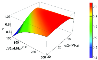
Figure 3: (color online). Fidelity versus $\Omega/2\pi$ and $g/2\pi$. The figure was plotted for $N=6$, $g_{12}/2\pi=0.1g$, $g_{1}=0.95g$, and $g_{2}=g$.

For a flux device with the four levels in Fig. 2(b), $g^{\prime}$ is on the same order of $g$ (or $g_{2}$). Thus, choose $g^{\prime}=g$ for simplicity. By the numerical test for $N=6$ and $\Omega/(2\pi)=300$ MHz [15], we find that for $g/\left(2\pi\right)\leq 15$ MHz [16], when $g_{12}\leq 0.1g$, the effect of inter-cavity crosstalk on the operation fidelity is negligible. Therefore, set $g_{12}=0.1g$ for Figs. 3 and 4 below. The condition $g_{12}\leq 0.1g$ can be met as discussed in [11].

Fig. 3 is plotted for $N=6$, showing that $\left\{{\mathcal{F},\Omega/\left(2\pi\right),g/\left(2\pi\right)}\right\}$ are: (i) 0.935, 300 MHz, 4 MHz; (ii) 0.916, 200 MHz, 10.5 MHz; and (iii) 0.870, 100 MHz, 6.5 MHz. These results indicate a high fidelity can be achieved for $N=6$. To further see how the fidelity varies with $N>6,$ Fig. 4 is plotted for $N\leq 10$ and different $\Omega.$ Fig. 4 shows that for $N=10$, $\left\{{\mathcal{F},\Omega/\left(2\pi\right),g/\left(2\pi\right)}\right\}$ are: (i) 0.864, 300 MHz, 9 MHz; (ii) 0.827, 200 MHz, 7 MHz; and (iii) 0.743, 100 MHz, 4 MHz. The $g$ values here were obtained by numerically optimizing the coupling constants. These results indicate a high fidelity can be obtained even for $N=10$.

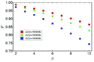
Figure 4: (color online). Fidelity versus $N$. The figure was plotted for $g_{12}/2\pi=0.1g$, $g_{1}=0.95g$, and $g_{2}=g$.

For cavities $1$ and $2$ with frequencies given above and the $\kappa_{a_{1}}^{-1}$ and $\kappa_{a_{2}}^{-1}$ used in the numerical calculation, the required quality factors for the two cavities are $Q_{1}\sim 4.4\times 10^{5}$ and $Q_{2}\sim 6.9\times 10^{5},$ which are readily available in experiment [17]. Our analysis given here demonstrates that high-fidelity generation of the NOON states with $N\leq 10$ even for the imperfect device is possible within the present circuit QED techniques.

This work was supported in part by the National NSFC and BRPC under Grant Nos. [11074062, 11374083, 11375003, 11174081, 11034002, 11134003, 2011CB921602], the funds from Hangzhou Normal University under grant Nos. [HNUEYT 2011-01-011, HSQK0081, PD13002004], and the funds of Hangzhou City for the Hangzhou-City Quantum Information and Quantum Optics Innovation Research Team.

References

(1) A. N. Boto, P. Kok, D. S. Abrams, S. L. Braunstein, C. P.
Williams, and J. P. Dowling, Phys. Rev. Lett. 85, 2733 (2000).
(2) P. Kok, H. Lee, and J. P. Dowling, Phys. Rev. A 65,
052104 (2002).
(3) I. Afek, O. Ambar, and Y. Silberberg, Science 328,
879 (2010).
(4) C. H. Bennett and B. D. DiVincenzo, Nature 404, 247
(2000).
(5) A. Blais, R. S. Huang, A. Wallraff, S. M. Girvin, and R. J.
Schoelkopf, Phys. Rev. A 69, 062320 (2004).
(6) J. Q. You and F. Nori, Nature 474, 589 (2011); Z. L.
Xiang, S. Ashhab, J. Q. You, and F. Nori, Rev. Mod. Phys. 85, 623
(2013).
(7) F. W. Strauch, K. Jacobs, and R. W. Simmonds, Phys. Rev. Lett.
105, 050501 (2010).
(8) S. T. Merkel and F. K. Wilhelm, New J. Phys. 12,
093036 (2010).
(9) H. Wang, M. Mariantoni, R. C. Bialczak, M. Lenander, E.
Lucero, M. Neeley, A. D. O’Connell, D. Sank, M. Weides, J. Wenner, T.
Yamamoto, Y. Yin, J. Zhao, J. M. Martinis, and A. N. Cleland, Phys. Rev.
Lett. 106, 060401 (2011).
(10) F. W. Strauch, Phys. Rev. Lett. 109, 210501 (2012).
(11) Q. P. Su, C. P. Yang, and S. B. Zheng, Scientific Reports
4, 3898 (2014).
(12) J. Clarke and F. K. Wilhelm, Nature 453, 1031 (2008).
(13) J. Q. You and F. Nori, Phys. Today 58, 42 (2005).
(14) M. Stern, G. Catelani, Y. Kubo, C. Grezes, A. Bienfait, D.
Vion, D. Esteve, and P. Bertet, Phys. Rev. Lett. 113, 123601 (2014).
(15) M. Baur, S. Filipp, R. Bianchetti, J. M. Fink, M. Göppl, L.
Steffen, P. J. Leek, A. Blais, and A. Wallraff, Phys. Rev. Lett. 102, 243602 (2009).
(16) T. Niemczyk, F. Deppe, H. Huebl, E. P. Menzel, F. Hocke, M.
J. Schwarz, J. J. Garcia-Ripoll, D. Zueco, T. Hümmer, E. Solano, A. Marx,
and R. Gross, Nature Physics 6, 772 (2010).
(17) P. J. Leek, M. Baur, J. M. Fink, R. Bianchetti, L. Steffen,
S. Filipp, and A. Wallraff, Phys. Rev. Lett. 104, 100504 (2010).