detection of stars within 0.8” of Kepler objects of interest
Abstract
We present an algorithm to search for the faint spectrum of a second star mixed with the spectrum of a brighter star in high resolution spectra. We model optical stellar spectra as the sum of two input spectra drawn from a vast library of stars throughout the H-R diagram. From typical spectra having resolution of R=60,000, we are able to detect companions as faint as 1% relative to the primary star in approximately the V and R bandpasses of photometry. We are also able to find evidence for triple and quadruple systems, given that any additional companions are sufficiently bright. The precise threshold percentage depends on the SNR of the spectrum and the properties of the two stars. For cases of non-detection, we place a limit on the brightness of any potential companions. This algorithm is useful for detecting both faint orbiting companions and background stars that are angularly close to a foreground target star. The size of the entrance slit to the spectrometer, 0.87 x 3 arcsec (typically), sets the angular domain within which the second star can be detected. We analyzed Keck-HIRES spectra of 1160 California Kepler Survey objects of interest (KOI) searching for the secondary spectra, with the two goals of alerting the community to two possible host stars of the transiting planet and to dilution of the light curve. We report 63 California Kepler Survey objects of interest showing spectroscopic evidence of a secondary star.
Subject headings:
— stars: single — binaries: spectroscopic, planetary systems — techniques: spectroscopic, radial velocity, statistical1. Introduction
One of the Kepler Mission’s main goals is to determine the abundance of the terrestrial and larger planets in the habitable zone, to characterize their orbits, and to determine their physical properties. As of February 27, 2012, the catalogue of Kepler Planetary Candidates has 2300 entries (Batalha et al. 2013). Planet candidates are identified by their photometric signals and then confirmed by additional photometric and spectroscopic analysis. However, it is well known that roughly half of all star systems are actually binaries or triples (Raghavan et al. 2010). Therefore, it is likely that roughly half of the Kepler Planetary Candidates have two or more possible host stars. At the typical distances of Kepler objects of interest (KOIs) of 0.3 - 1.0 kpc, orbiting stellar companions with typical orbital distances of 5 - 500 AU would be unresolved from the primary stars. This implies that roughly half of the Kepler Planetary Candidates have a major ambiguity about the nature of the host star of the transiting: it could be any of the stars in the binary or triple star system. Moreover, even if the planet transits the primary star, the dilution of the Kepler photometry from the secondary and tertiary stars causes an underestimate of the radius of the planet. Such an ambiguity can also be caused by a background star, angularly close to the Kepler target. The identification of a second set of absorption lines in the spectrum of a KOI highlights cases with such ambiguities and casts appropriate uncertainty on the measured radii of the planets.
Besides the dilution of the Kepler light curve, there is also a possibility that what appears to be a planet is in fact a false positive. This is a serious concern for the Kepler mission, as there are numerous astrophysical phenomena that can produce the dimming indistinguishable from that of the transiting planet. A few such examples are the grazing eclipsing binaries, a giant primary star eclipsed by a dwarf, or a background star. The first two cases can usually be identified by the photometry alone, but the background stars pose further challenges to planet validations, particularly for cases of background eclipsing binaries. There is also another case, especially important to consider for smaller planet candidates. The amount of dimming caused by an Earth-like planet orbiting a Sun-like star can be mimicked by a larger planet orbiting a background star, or a less bright binary system companion.
All these alternative situations drastically alter the interpretation of the phenomena that caused the dimming detected by the Kepler spacecraft, and significant efforts have been made to characterize the false positive probability (FPP) among the Kepler planet candidates. The values in the literature range from FPP 10% (Morton & Johnson 2011; Fressin et al. 2013), to 35% (Santerne et al. 2012) for giant planets. Even the lowest estimated FPP is high enough to raise concerns about individual planet discoveries. In an effort to decrease FPP we developed a method for detecting faint stellar companions in double-lined spectroscopic binaries.
In this paper, we present a spectroscopic method of searching for a secondary set of absorption lines in a spectrum. A detection of such lines would reveal a secondary star close enough for its light to reach the aperture and affect interpretation of the phenomena responsible for the dimming. The entrance slit has angular dimensions projected onto the sky of 0.87” x 3.0”. The slit is oriented differently for each exposure, with the primary star centered on the slit in both dimensions. A secondary star will be included in the spectrum if it resides anywhere within the slit, which restricts the maximum angular separation between the primary star and the secondary star at 0.43” to 1.5”, depending on the orientation of the slit. Most commonly, the secondary star is oriented relative to the primary star at a typical angle of 30 to 60 degrees to the length of the slit, in which case its light will be collected if it resides within 0.5” to 0.8” from the primary star.
Our goal is to detect any bound or non-bound secondary star as faint as 1% relative to the primary target star, with either sufficiently large relative radial velocity to allow for the Doppler separation of the two sets of absorption lines, or with sufficiently different spectral features to allow for the differentiation among the overlapping spectral lines. The presence of such a star does not prove that the transit signal is not a planet. It merely indicates that a second star is located within 0.5” 0.8” of the primary star, causing ambiguity about the host star and uncertainty about the planet radius.
A standard tool for spectroscopic binaries is TODCOR (Mazeh et al. 1993), used extensively to model, self-consistently, the two underlying spectra in a given spectrum. This code has been shown to provide excellent detection and assessment of the properties of the two stars. We, however, wanted to develop our own method for detecting secondary lines with a primary goal of being extremely conservative in our detections. We adopted an ”Occam’s Razor” approach in which any observed spectrum of just one star would be deemed a sufficient model. We only invoke the spectrum of a second star in the model if absolutely forced to do so by the residuals that show the second star to be statistically significant. Thus, we seek an algorithm that accomplishes a statistically robust identification of secondary lines. We were dedicated to constructing an algorithm that we understand in precise detail, and consider our intimate knowledge of our own algorithm to be vital in assessing its integrity and functionality.
2. Spectrum Preparation
We worked with spectra from HIRES at Keck Observatory. HIRES has a bandwidth that covers wavelengths from 3643 to 7990 . We worked with the wavelength region from 4977 to 7990 , avoiding the parts of the spectrum polluted by telluric lines as well as the region of the interstellar sodium D lines. This wavelength domain encompasses approximately the V and R broadbands of classical photometry.
Using one of the 0.86”-wide slits, HIRES has a resolving power of 60,000 at 5500 . The SNR of the spectra depends on the brightness of the primary star and the duration of the exposure. The typical SNR values range from 45 to 200 per pixel.
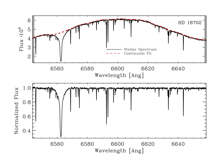
First, we continuum-normalize each HIRES spectrum to remove the somewhat variable blaze function from each spectral order. We fit the continuum using the fifth order polynomial, divide the spectrum by the fit and thus obtain a flat continuum at unity, shown in Figure 1.
Once flattened, we resample the spectrum on a constant wavelength scale, using interpolation. We are using a wavelength scale with a pixel spacing of 1.3 . Resampling is done by using a set prescription of converting HIRES pixels into intervals. This wavelength scale allows for a simpler relationship between the pixel positions of absorption lines and the Doppler shift of the star; with spectrum on a constant scale, a Doppler shift of corresponds to a simple translation of the spectrum for = ( )/1.3.
3. The Search Algorithm for a Faint Secondary Spectrum
3.1. Fitting the Spectrum of the Primary Star
Since we are interested in the relative radial velocity between the primary star and the potential companion, we correct for the Doppler shift of the primary star such that the primary star’s absorption lines reside at the rest frame wavelengths. We determine the Doppler shift of the primary star using the statistic of cross-correlating the corrected NSO Solar spectrum (Wallace et al. 2011) with no Doppler shift. We determine the location of the minimum, which corresponds to the radial velocity at which the absorption lines of the Sun’s spectrum align with the absorption lines of the primary star - the primary star’s Doppler shift. Since we are using a wide range of wavelengths, the discrepancy in the spectral type between the Sun and the star in question does not cause any difficulties in determining the radial velocity of the primary star.
3.1.1 Finding the Best-Fit
Once the spectrum is normalized and on a constant wavelength scale, we search through the SpecMatch library of stellar spectra in order to find the best fit for the primary star. The SpecMatch library consists of Keck-HIRES spectra of 640 FGKM stars scattered throughout the H-R Diagram, with a concentration to the main sequence and subgiants. These spectra were obtained as part of the California Planet Search. Each spectrum has SNR=100-200 per pixel between 3800-8000 with the same spectral resolution as the bulk of the spectra analyzed here, R=60,000.
All of the SpecMatch library spectra are available online at the Keck Observatory Archive. Apart from M-dwarfs, each spectrum was analyzed with an advanced version of the spectroscopic analysis package, SME, described in Valenti & Fischer (2005). SME was later modified based on the available parallax information, toward a revised, improved version of SME (Brewer et al. 2014, in prep). This analysis yielded the values of , log, and [Fe/G] for all FGK stars in the library. Stellar parameters for M-dwarfs were adopted from Rojas-Ayala et al. (2012).
SpecMatch stellar parameter values range in =[3250,7260], log=[1.46,5.00], and [Fe/H]=[-1.475,0.558]. We assume that the primary star lies on main sequence and exclude the subgiants from the library as possible best-fit candidates. This choice was made due to the preferential choice of subgiants as the best-fitting stars, even when the observed primary star was on main sequence. Excluding the giants improves the quality of the best-fit and allows for a better subtraction of the primary spectrum, which is explained in Section 3.3.1. This decision was made with an objective of our efforts in mind; since our primary goal is to search for the secondary lines in the spectrum, we sacrifice some of the accuracy of the primary star parameters in order to achieve a better fit to the primary star absorption lines. Nevertheless, if the spectral type of the primary star is known, the algorithm can be modified to include the subgiants in the fitting process as well.
We look for the library spectrum that produces the lowest value when the absorption lines of the library spectrum are aligned with the studied spectrum. We vary both the rotational broadening of each library spectrum as well as the depth of the absorption lines by diluting the spectrum. The latter is to correct for the finite grid spacing of the metallicity in our library, and is implemented to ensure as complete subtraction of the primary star absorption lines as possible. Due to the inclusion of the constant dilution factor, we are unable to determine the log of the primary star altogether. However, as mentioned above, the determination of the parameters for the primary star is beyond the scope of this paper, and can be performed using a different method, if so desired.
Taking above into account, the is computed using
| (1) |
where is the SpecMatch library spectrum, is the rotationally broadened observed spectrum, is the dilution factor, and is the Doppler shift of the primary star in pixels.
Discrepancies between each library star and the actual spectrum are both due to Poisson noise as well as intrinsic spectral differences. This is mostly due to the finite grid spacing in parameter space of our library. As a consequence, we cannot establish a good uncertainty estimate for each point along the spectrum, and the actual value of bears no significance; rather, it is the relative among all of the library spectra that we are concerned with.
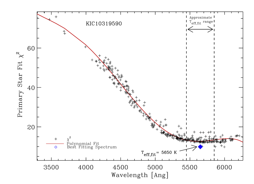
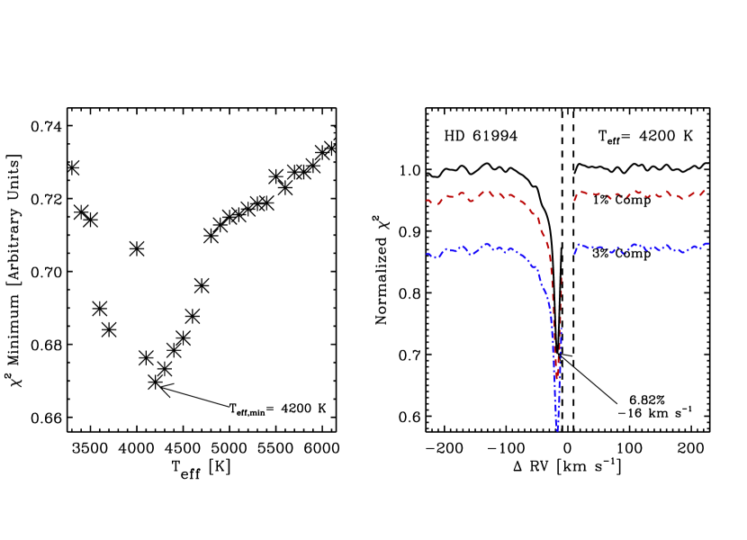
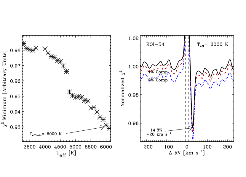
In order to prevent outliers to be identified as best-fitting stars, we first identify the approximate temperature of the primary star by finding the minimum of the versus library star temperature distribution, as shown in Figure 2. The vertical scatter of the points at the same is due to the discrepancies in other parameters, such as log and metallicity. Note that we could plot as a function of other parameters as well; we choose the temperature as the distribution the has most easily identifiable minimum.
Based on the polynomial fit to the distribution, we then eliminate the outliers that differ from the polynomial fit for more than 3 at any value of the effective temperature. We then repeat the polynomial fitting, and choose the lowest value within the 200 K range about the minimum of the polynomial fit as our best-fitting library spectrum. While restricting the range of possible to 200 K around the polynomial minimum might introduce larger uncertainty in the determined of the primary star, it does ensure that the chosen library spectrum is the best achievable fit to the observed spectrum and has approximately correct effective temperature. Restricted range excludes any outliers that have not yet been eliminated at the edges of the effective temperature range (6100K and 3400) due to the edge effects on the shape of the polynomial.
Since the main goal of the primary star fitting is the subtraction of its absorption lines from the spectrum, we do not report any of the best-fit parameters for the primary star. The accuracy of these results is compromised due to several manipulations of the library spectra to account for the finite grid of our library parameter space. Nevertheless, all of the steps described above do ensure that the primary star absorption lines are fitted almost perfectly and subtracted almost completely. If the parameters for the primary star are known, however, any or all of the values in the parameter space we search over (log, , rotational broadening, ) can be constrained to a known range or fixed to a known value.
3.2. Bright Secondary Stars
Brighter stellar companions (10% relative brightness) can be detected using primary as a function of Doppler shift. We use the same function we used for determining Doppler shift of the studied star, described in Section 3.1. As mentioned in Section 3.1.1, the actual values are of no significance. Therefore, we normalize function such that its median value is one when the lines of the NSO Solar spectrum and studied spectrum are misaligned. Deviations from unity are due to the accidental alignments of absorption lines with those corresponding to a different element.
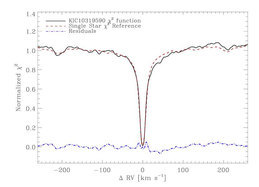
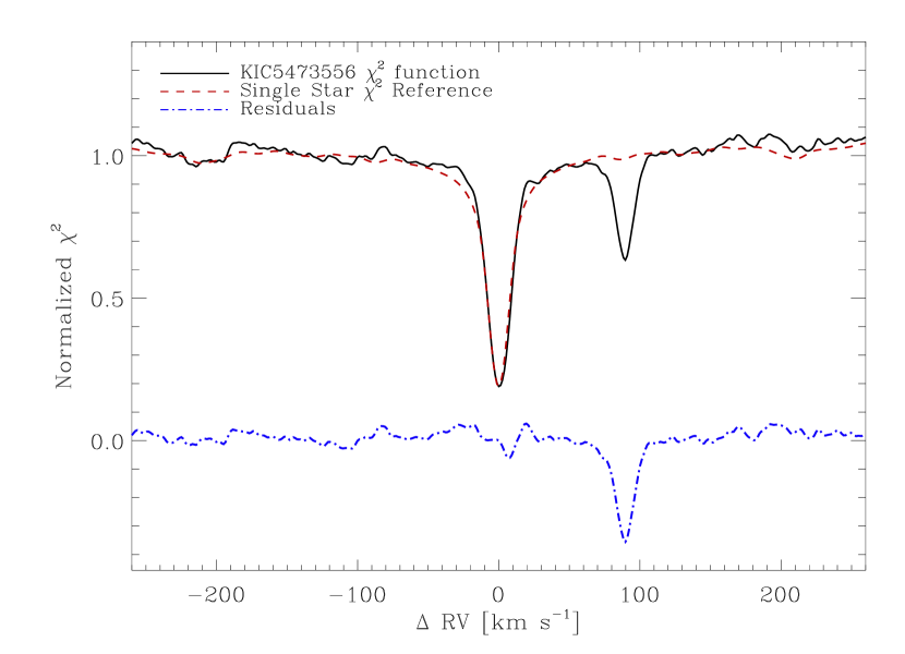
We noticed a trend in those accidental alignments that was independent of the spectral type for the primary star, as all of the primary functions had the same shape outside the central minimum. We thus created a function by cross-correlating the Sun’s spectrum with itself, and adopted this shape as the characteristic single star function. We then compare the actual function to this characteristic single star function in order to detect any discrepancies with might indicate the presence of a companion, as shown in Figure 3.
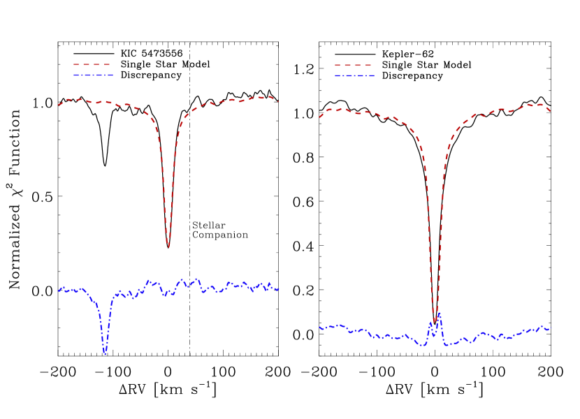
We can see in Figure 3 that the primary function reveals a secondary star of KIC 5473556 (at left), at a relative RV of +90 . Such detections are only possible when the secondary star is sufficiently bright with a large enough relative velocity. The dip has a FWHM width of approximately 20 , thus any secondary star with a RV 10 would blend in and remain undetectable. Due to variable rotational broadening of the lines among different spectra, we artificially broaden the characteristic single star function to match the width of the actual for the analyzed spectrum. Thus, the detection threshold of the relative brightness for the secondary star varies both with RV and the nature of the star’s spectrum.
3.3. Faint Secondary Stars
3.3.1 Subtraction and the Residuals
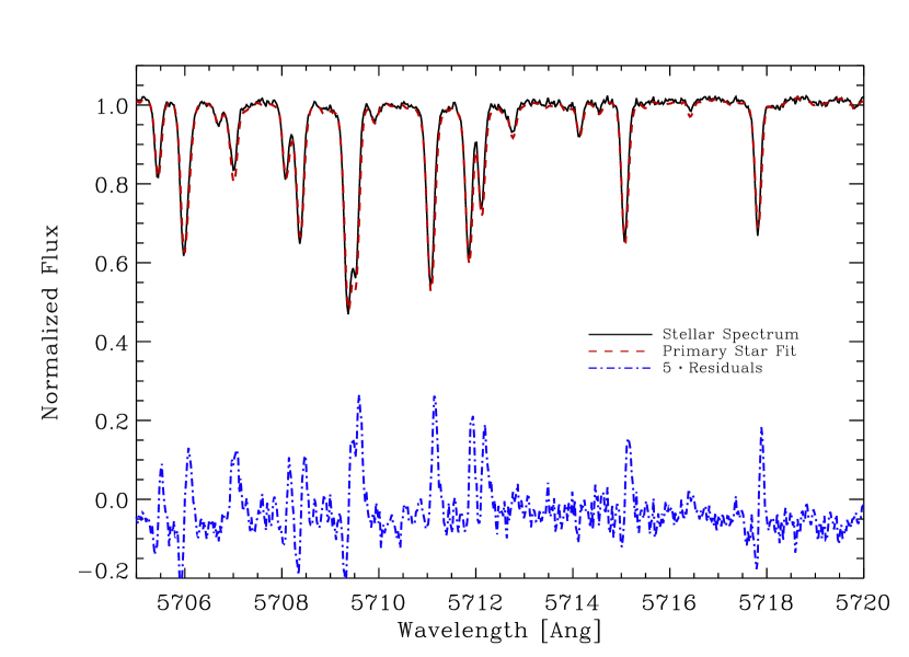
Once the best-fit library spectrum is identified and its lines both broadened as well as diluted to match the primary star’s absorption lines, we subtract that best-fit library spectrum from the original spectrum, leaving residuals as shown in Figure 4.
3.3.2 Evidence of Secondary Lines
We re-normalize the residuals described above back to unity, and search for the secondary set of absorption lines. Since our algorithm is focused mostly on faint secondary stars, the spectral differences among two stars with K are almost indiscernible. To enhance efficiency, we create 26 median spectra with intervals of 100 K starting at 3300 K and up to 6100 K, rather than utilizing each individual library spectrum.
We omit where there are less than three spectra per 100 K temperature interval. As a consequence, not all of the 100 K temperature intervals are represented. In particular, we do not have a representative median library spectrum at effective temperature 3800 K and 3900 K.
We then calculate as a function of Doppler shift between the residuals and each median library spectrum, and normalize it such that the median is 1. A significant minimum occurring at the same for several neighboring effective temperatures of the median library spectrum indicates a possible second star in the spectrum. An example of a residual function is shown in Figure 5.

Unless the primary and the secondary spectrum are sufficiently different, we cannot detect secondary stars with 10 relative to the primary star due to the normal widths of the absorption lines. Since none of the library spectra are the exact match to the studied one, there will always be some imperfections in the best-fitting library star, resulting in larger residuals at the locations of primary star’s absorption lines. These residuals may cause either small peak or a small dip at = 0 . Thus, if both stars have exactly the same radial velocity, we cannot differentiate between the minimum at = 0 that is due to the imperfect subtraction of the primary, or the one due to an actual second star. Furthermore, secondary sets of absorption lines with slightly different radial velocities than the primary star have their spectral lines still blended with the primary star’s absorption lines. This occurs if the RV separation is less than 10 , the typical width of an absorption line. This blending causes a fraction of secondary absorption lines to be subtracted away together with the primary star, making a faint second star appear even fainter, and in most cases impossible to detect.
Due to the limitations described above, we mask out the central region with 10 , as shown in Figure 6. The only exception is the case where the two spectral types are sufficiently different that primary star spectrum does not interfere with the secondary, regardless of their RV separation. This is the case of a G-type primary and an M-dwarf secondary star, further discussed in Section 4.1.4.

3.3.3 Estimating Secondary Star Temperature
As mentioned in Section 3.3.2, we obtain 26 distinct residual functions, differing in the effective temperature of the library spectrum superimposed with the studied residual spectrum. We expect to find a unique location of the secondary star, if one is detectable. Since a secondary set of absorption lines would cause a minimum in over a range of library spectral types that are close in to the actual temperature, we assume the secondary star to be the mode of the minimum locations for a set of all 29 residual functions. The exception here is the case where the minimum occurs only for 3500 K. Due to a significantly different M-dwarf spectrum, it is possible that the secondary star is detected only in a few residual functions with 3800 K. Those cases are examined and assessed on an individual basis.
Using the mode minimum location, we plot the values at those locations versus the temperature of the median library spectrum used to construct each respective function. For most residual functions, this is indeed the minimum. Ideally, the depth of the minimum should only depend on how well the library spectrum correlates with the spectrum of the secondary star, producing the lowest minimum when the library spectrum temperature is closest to the effective temperature of the secondary star. However, mostly due to the low SNR of the residuals, we noticed a dependence of the residual minimum on the temperature of the library spectrum that was independent of the actual of the secondary star. In order to correct for this, we divide the minima plot by the calibration function, construction of which is described in more detail in Section 4.1.2.
We then plot the calibrated minimum values versus the temperature of the median library spectrum, as shown in Figure 9 (left). In order to determine approximate temperature of the secondary star, we follow the same procedure as for the primary star, outlined in Section 3.1.1. In brief, we fit the points with a polynomial, find a minimum, remove the outliers that differ from the fit by more than 3 , re-fit the remaining points, and restrict the possible range of secondary star to 200 K around the polynomial minimum. Within that range, we then compute the mean of the three median library spectra corresponding to the three lowest minima. We adopt this mean as the estimated temperature of the secondary star. Taking the mean of the three lowest values corrects for the missing median templates, as not every 100 K is represented due to varying parameter populations of SpecMatch library.
We cannot extrapolate the behavior of the minima function to values of higher than 6100 K or lower than 3300 K. Thus, any secondary stars whose is identified at 6000 K is not guaranteed to be at that temperature; rather this serves as the lower temperature limit, as the secondary star can be hotter than 6000 K but not cooler. Similarly, secondary stars whose estimated is 3300 K can be cooler than this value, but not hotter. This is discussed more in detail in Section 6.2.
3.3.4 Estimating Relative Brightness
After determining of the second star, we use the corresponding residual function for further analysis. We aim to estimate the brightness of the secondary star relative to the primary star based on the depth of that residual function minimum.
We do so by synthesizing the effect of secondary spectra. We inject another spectrum into the original studied spectrum. We scale down the injected spectrum such that it contributes either 3% or 1% of the total flux, and shift its absorption lines to a known relative radial velocity. The injected spectrum has close to that already estimated for the secondary star temperature, assuring that the superimposed library spectrum fits both the actual secondary star as well as the injected spectrum equally well. The properties of all the possible injected spectra are listed in Table 1.
We then treat this original spectrum, with its synthetic injected secondary star spectrum, as the new studied spectrum, and repeat the whole procedure outlined in Sections 3.1.1 through 3.3.2. We record the value at the location of the injected spectrum, annotated in Figure 7. At that particular , the difference between the injected spectrum and the value of the original , both shown in Figure 7, represents the minimum depth would be caused by a secondary star of the injected brightness.
To obtain a more statistically useful sample of possible secondary spectra, we repeat the injection for several different values s, and each time record the difference between the value of the minimum at the location of the injected secondary spectrum and the original residual value at that location. Using those differences, we then calculate the median minimum depth relative to the original residual caused by a secondary star of that particular brightness.
Subtracting the median depth for both 3% and 1% injected secondary spectrum from the original residual without the injected secondary spectrum, we obtain the plot shown in Figure 8. At each , the two colored curves represent the value that the function would have if there was a secondary star of the specified brightness located at that particular . This allows for a visual comparison of the actual residual minimum to the characteristic minima depths for 3% and 1% secondary stars.
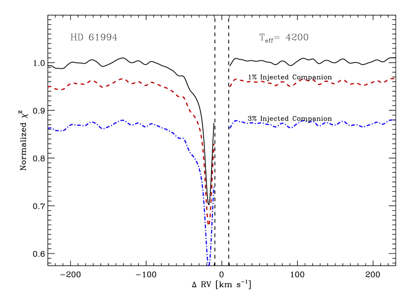
To estimate the relative brightness of the actual secondary star, we extrapolate the median minimum caused by the 3% and 1% injected secondary spectrum to the actual minimum for the residual function. We use a least-squares linear fit, with a restriction that 0% secondary star (none present) causes a minimum of depth 0. We report both the of the secondary star, as well as the estimated relative brightness as a percentage of total flux, on the plot.
Since our wavelength domain encompasses approximately the V and R broadbands of the classical photometry, the relative brightness of the two stars can be used to compute the dilution factor of the Kepler light curves. Thus, if the primary star has any planet candidates, this dilution factor can help determine a more accurate radius of the planet.
3.3.5 Secondary Star Detection Summarized
Figure 9 has two panels, the left showing the calibrated residual minimum as a function of and the right showing vs. RV. This includes the minima curves for 1% and 3% injected secondaries, shown in red and blue respectively (see Section 3.3.4).
This final Figure 9 is intended to summarize our knowledge about the secondary star: estimated , estimated percentage contribution to the total flux spectrum in the V and R bands, and the radial velocity of the secondary relative to the primary star. Any additional parameters for the secondary star cannot be determined accurately enough to be published.
On the final secondary star plot, we annotate any minimum that contributes at least 0.5% of the total flux. Depending on the SNR of the original spectrum (typically 50-200 per pixel), the spectral types of the two stars, and their , secondaries with fluxes between 0.5% - 1% relative to the primary star can be detected with our algorithm.
We visually inspect each diagnostic plot to assess the probability that the identified minimum is indeed due to a secondary star. When there is no clear minimum, or when the minimum is due to fluctuations, we establish the threshold limits on the secondary star as follows. Any undetected secondary must contribute less to the total flux than would have been revealed above the fluctuations in the functions. If this percentage is not marked on the plot, the brightness limit is 0.5% relative to the primary star. Otherwise, the appropriate percentage is marked on the plot. M-dwarf secondaries contributing more than 0.5% of the total flux can be typically detected in our spectra if present, or ruled out if not present.
4. Assessing the Algorithm: Tests of Synthetic and Real Binaries
4.1. Injection-Recovery Experiment
In order to test and calibrate our algorithm, we performed injection-recovery experiments. The goals were to estimate the uncertainty for the determined secondary star parameters, allow for the correction of any systematic errors, and identify the limitations of the algorithm.
We synthesized three sets of 360 binary stars, composed of pairs of our library spectra with added 2% Poisson noise. The noise level reflects that (2% per pixel, i.e. SNR45) common to many of the Keck-HIRES spectra we analyzed in this paper, namely the 1160 Kepler Objects of Interest, described in Section 5. Since the spectra used to synthesize the binaries are real, observed spectra with Keck-HIRES, they already contain a certain amount of other types of noise (such as red noise), and thus the synthetic binaries accurately capture the nature of any other spectra analyzed in this paper.
We chose library stars in increments of 500 K, ranging from 3500 K to 6000 K. We then created pairs of spectra for all possible permutations of , beginning at 3500 K for both the primary and the secondary star. We considered all possible combinations, including those where the primary star is cooler than the secondary, to account for both bound systems and background companions. The secondary set of absorption lines was shifted from the primary by of 50 , where the two sets of lines are well separated. Tests have shown that for separations larger than 10 the detectability of the second star is independent of the relative radial velocity for the two stars. For smaller separations, the two sets of absorption lines overlap due to the natural broadening. At such small separations, we can only detect M-dwarf secondary to a G-type primary star. For those cases, additional tests have been carried out with the secondary set of absorption lines shifted from the primary by only 5 .
Each of the three sets of 360 spectra differs by the relative brightness of the secondary star. We constructed cases in which the second star contributed 10%, 3%, and 1% of the total flux in our optical spectra (V and R bandpasses). For the cases of G-type primary and an M-dwarf secondary star we performed additional tests with even higher flux ratios, where the M-dwarf secondary star contributed as low as 0.05%, 0.1$ and 0.5% of the total flux. To obtain statistically significant sample, we created 10 different binary spectra for each such permutation, each with a different realizations of Poisson noise. We then blindly executed our search algorithm for secondary spectra on each synthetic binary. In the search, we removed the spectra used to construct that particular case from the library, preventing those to be chosen as best fitting stars.
4.1.1 Secondary Star Recovery Rate
We used the synthetic binary spectra with added noise to determine the uncertainties in the deduced parameters for the secondary star. We investigated each temperature combination, as well as each flux ratio, separately. We examined the recovery rate by counting all the cases where the secondary star was identified, disregarding the accuracy of the estimated parameters. Results are summarized in Table 2. The Table can be read as follows: values running horizontally denote the effective temperature of the secondary star, and the values running vertically down the first column denote of the primary star. For example, 60% rate quoted in the last column of the first data row means that the secondary star in the binary spectrum consisting 99% of a 3500 K star and 1% 3500 K star was successfully identified in 6 out of 10 cases.
For all synthetic spectra, we added a Poisson noise at the level of 2%. Since we subtract the primary star absorption lines, a 1% secondary implies an SNR for the residual spectrum of only 0.5, 3% has an SNR of 1.5, and 10% secondary yields a residual spectrum with SNR of 5. Of course, such low SNR values per pixel are overcome by the thousands of absorption lines, detected in thousands of pixels, each contributing to the detectability of the secondary star. Thus the effective signal-to-noise of the secondary star is much higher than the per-pixel SNR.
4.1.2 Calibration of the Secondary Star Temperature
We isolated the synthetic binary cases where the binarity of the spectrum was established, and examined the predicted secondary star temperature as opposed to the actual values. As mentioned in Section 3.3.3, we noticed a dependence of the depth of the residual minimum on the temperature of the library spectrum, which was superimposed with the studied spectrum to construct the residual . Except when the secondary star was an M-dwarf, the residual minimum was always the deepest for 4500 K, regardless of whether or not that was the actual of the secondary star. We suspect this bias is caused by the nature of the 4500 K spectrum itself, as it contains an abundance of deep and sharp absorption lines from neutral metals that dominate FGK spectra. With the primary star subtracted from the spectrum, the residuals are dominated by Poisson noise at a 2% level, especially so when the secondary star contributes only a few percent to the total flux. These neutral metal absorption lines tend to accidentally align with the noise much more frequently due to their deep, sharp features. Such accidental alignments cause a deeper minimum for the 4500 K library star with the studied spectrum of any , particularly so for the residuals with SNR values near unity.
This bias was strong enough to influence the estimated temperature of the second star and make our deduced raw derived secondary star parameters inaccurate. In order to correct for this temperature bias, we calculated the average residual minimum distribution for all of the test cases of a particular flux ratio, excluding non-detections. If the distribution was unbiased against library spectrum’s , the mean distribution should be a approximately constant with respect to temperature, as we assured that there were an equal number of cases at each secondary star .
We found, however, that this was not the case; the mean distribution peaked at 4500 K, as expected. Since the shape of any true minimum distribution will be affected by this peak, we use the mean distribution, normalized such that the maximum occurs at = 1, as our calibration function. Calibration functions for a 1%, 3%, and 10% secondary star are shown in Figure 10.
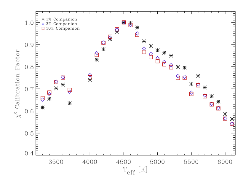
As we can see from Figure 10, calibration functions are almost identical among different relative brightnesses of the two stars. Therefore, there will be negligible errors resulting from dividing a residual minimum distribution by these calibration functions for cases where the relative brightness of the studied star is not 1%, 3%, or 10% exactly.
4.1.3 Secondary Star Parameters
Using calibrated minimum distribution, we estimated the second star temperature and relative brightness, as described in Sections 3.3.3 and 3.3.4. We then compared the deduced values to the known parameters, and the discrepancies are shown in Tables 3 and 4, respectively.
Table 3 lists the discrepancies in the SpecMatch value and the one derived from our algorithm, (). Table 4 lists the discrepancies in the set secondary star percentage contribution to the total flux and the value derived by our algorithm. We know the actual flux contribution precisely, as we artificially scaled down the secondary spectra when constructing synthetic binaries. The values are listed in terms of the percentage of the total flux, (). Each primary-secondary temperature combination consisted of 10 trial cases, with different realizations of added Poisson noise.
We report both the systematic difference (the mean discrepancy) as well as the associated standard deviation. Since the systematic differences are not constant over all temperature combinations or relative brightnesses, we cannot apply a single correction to obtain a more accurate values. As such, Tables 3 and 4 serve more as illustrations of the injection-recovery results.
We noticed larger systematic differences for 4000 K secondary stars. This is mostly due to the scarce SpecMatch library populations in that region, with some 100 K intervals missing altogether. On the other hand, the algorithm did consistently identify correctly the M dwarf secondaries, owing their detectability to their distinct spectral features. As expected, the systematic differences in as well as the standard deviations decreased for brighter secondary stars, as the secondary spectrum becomes brighter than the 2% noise.
On the other hand, absolute errors in percentage increased when the secondary star was brighter. This was expected, since the errors in linear extrapolations of minimum depth become larger for brighter stars. Nevertheless, the errors were still mostly around 1% only, and the relative errors rarely exceed 50%. We also noticed a pattern that relative brightness of hotter secondary stars was mostly overestimated, while cooler stars were underestimated. These trends can be useful when establishing limits on brightnesses of any real secondaries.
We combine both the systematic error and the uncertainty to form more conservative uncertainties to be used with the secondary star parameters deduced in the analysis of actual spectra. These are shown in Table 5. Columns two through seven show the absolute uncertainty in the effective temperature of the secondary star for several possible primary-secondary star pairs; columns eight through 13 show the relative uncertainty in the flux ratio. Based on the effective temperatures of the primary-secondary pair and their flux ratio, appropriate uncertainty for both the effective temperature of the secondary star and its relative brightness can be read from Table 5.
4.1.4 G-type Primary and M-dwarf Secondary Star
As a part of the injection-recovery experiment, we also examined more closely the case of a G-type primary star with a temperature of 5500 K and an M-dwarf secondary at 3500 K. Due to its low temperature, M-dwarf spectrum contains many molecular lines in the visible spectrum, quite distinct from the spectrum of FGK-type stars. As such, it is much easier to detect an M-dwarf secondary spectra, even when the for the two stars is low.
We considered a situation where the two stars are separated by only 5 , placing the secondary set of absorption lines into the masked-out region on our residual versus plot. We constructed three sets 20 different synthetic binary stars with a 5500 K primary and a 3500 K secondary star, the secondary contributing either 1%, 3%, or 5% of the total flux. We then executed the algorithm on each spectrum, determined the recovery rate, and calculated the discrepancies in the deduced and percentage flux. Results are shown in Table 6. Each companion percentage contribution sample consisted of 20 test cases.
These results quantify the ability of our algorithm to detect M-dwarf secondary stars even when the two sets of absorption lines overlap. Nevertheless, some of the M-dwarf absorption lines still get subtracted away together with the primary star, thus the relative brightness of the secondary was consistently underestimated for all cases. This suggests an important limitation on our algorithm; when the secondary stars are detected in the 10 region, the estimated relative brightness of the second star is more of a lower limit rather than an actual value.
Besides considering M-dwarf secondary stars with low separation, we also explored the detectability limit in terms of relative brightness of the two stars. We constructed synthetic binaries where the M-dwarf secondary contributed 0.05%, 0.1%, and 0.5% of the total flux. Recovery rate for the 0.5% M-dwarf secondary star was 40%, while none of the fainter companions were detected. Since all of the spectra had a 2% percent noise, this places the M-dwarf detectability to a SNR 0.25.
4.2. Known Real Spectroscopic Binaries
We executed our algorithm on several cases of known spectroscopic binaries. We then compared our results to those available in the literature. Results are summarized in Table 7 for the primary star parameters, and in Table 8 for the secondary. The uncertainties for the secondary star parameter are based on the Table 5. Even though we normally do not report the parameters of the primary star, we include them in this experiment. This is to demonstrate that even though our primary star parameters might carry larger errors and uncertainties than those derived using alternative methods, they still poses a sufficient accuracy for the purposes of the subtraction of the primary star absorption lines.
4.2.1 KIC 10319590
KIC 10319590 is a precessing eclipsing binary, with time-varying eclipse depths (Rappaport et al. 2013; Slawson et al. 2011). There is very little evidence of the secondary star in the function for the primary star shown in Figure 11, indicating that the secondary is faint.
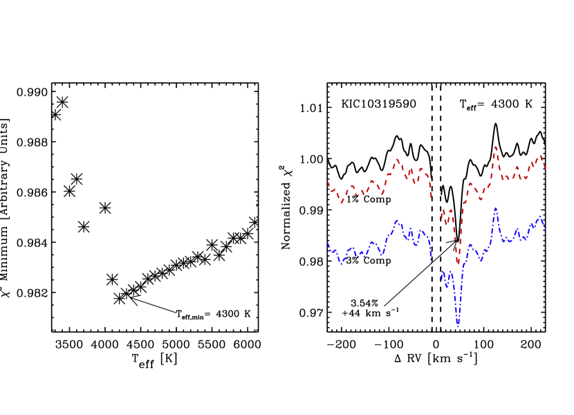
The residual function shown in Figure 12 shows an evidence of a secondary set of absorption lines at RV = +44 . Based on the residual minimum distribution, we estimate the secondary star = 4300 500 K, with uncertainty based on Table 5.
Deduced percentage of the total flux for the secondary star is 3.54%, yielding the flux ratio = 0.036 0.07. The comparison of our results to known parameters is limited by the lack of the available information.
4.2.2 KIC 5473556
KIC 5473556 is another example of a SB2 eclipsing binary (Angus 2013). For this system, the companion is sufficiently bright to cause a secondary minimum in the function for the primary star, shown in Figure 13.
There is a clear detection shown in the residual (Figure 14) at RV = +89 . We estimate the secondary star at 6000 100 K. At the relative flux of = 0.22 0.07, this could either be a bound companion or a background star, as the primary star is similar to the estimated secondary star value.
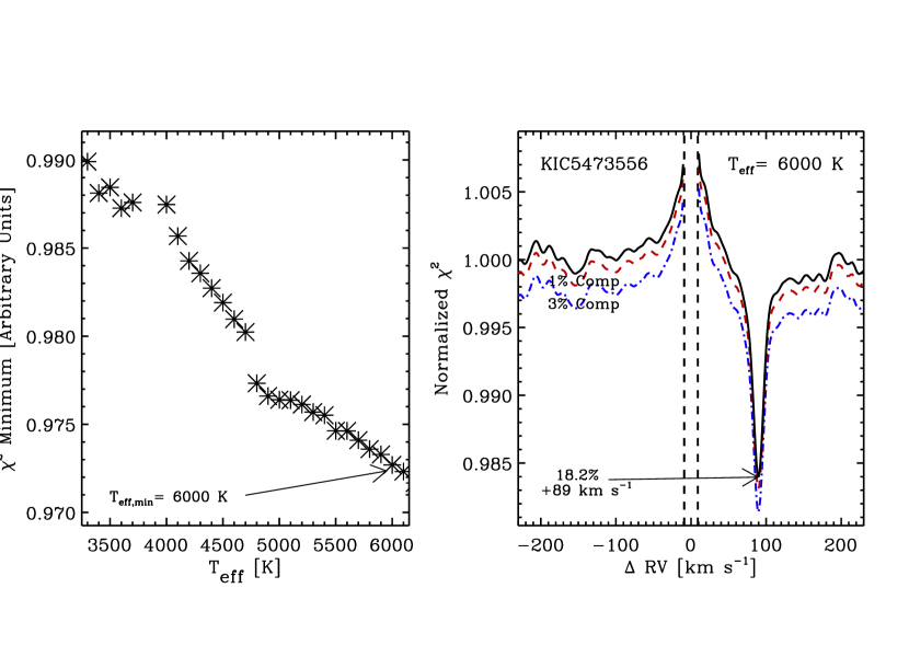
In order to resolve the ambiguity, we executed our algorithm using a different observation taken at a different time. If the two stars indeed orbit each other, a different orbital phase should yield a different value. This was indeed the case, as another observation shows a companion at -115 .
The flux ratio of 0.22 0.07 and an approximately the same for the two stars indicates that our deduced companion temperature might be an overestimate, and the actual companion most likely lies at the lower uncertainty limit, 5900 K. Moreover, it is possible that only a fraction of the flux from the companion actually entered the slit during the observation. Since the parameters for the companion of KIC 5473556 are not known, we cannot compare our derived flux ratio, = 0.22 0.07, to a known value.
4.2.3 KIC 8572936
KIC 8572936 is an SB2 binary system, also known for its circumbinary planet, Kepler-34 (Welsh et al. 2012). The two stars are both Sun-like stars, and their fluxes are comparable; =0.84750.005 (Welsh et al. 2012). The effective temperatures of the two stars are similar, = 5932130 K and = 5867130 K.
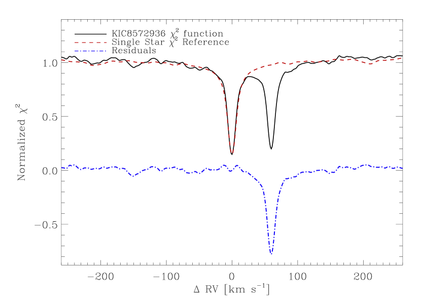
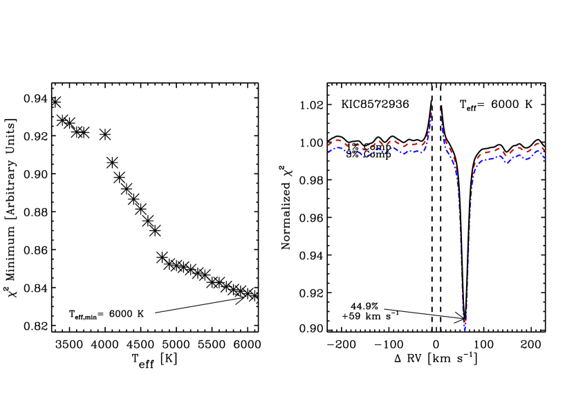
This is an interesting case due to the similarity between the two stars, both in their spectral types as well as in the fractional contribution to the total flux. The main problem with such cases is that the two sets of absorption lines interfere with the best-fit for the primary star, thus we inevitably subtract some of the secondary lines together with the primary star. This leads to a somewhat larger uncertainty in the derived flux ratio for the stars using our method; however, the detection of both stars is clear and unambiguous, as seen in Figure 15 and 16.
The estimated temperature of the companion of = 6000 100 K, is in agreement with = 5812 150 K quoted by Welsh et al. (2012). We calculated the flux ratio of = 0.82 0.25, which, in the uncertainty limit, also matches the Welsh et al. (2012) value of 0.8475 0.005.
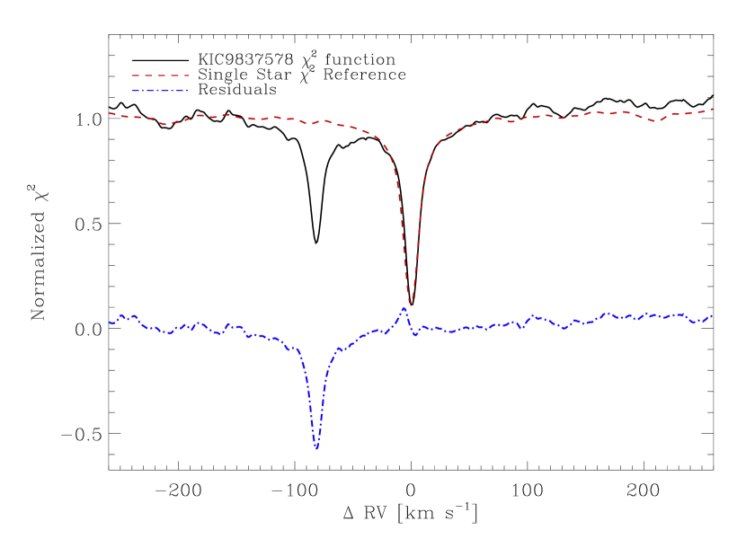
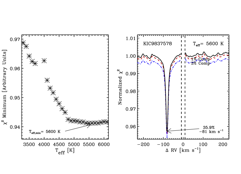
4.2.4 KIC 9837578
The case of KIC 9837578 is a similar to KIC 8572936. It is also an SB2 binary system, with the two stars of similar , but the flux ratio in the Kepler bandpass is somewhat lower, = 0.3941 (Welsh et al. 2012).
We find a secondary star at RV = -81 , with the estimated effective temperature of 5600 400 K (Figures 17 and 18). Taking into account the uncertainty, agrees with Welsh et al. (2012) value of 5202 100 K. The estimated flux ratio for the two stars of 0.56 0.14 is larger than the Welsh et al. (2012) value by 7%. Some of this discrepancy can be attributed to slightly different wavelength bandpass of our spectra as compared to Welsh et al. (2012), and some due to the mixing of the two sets of absorption lines as both stars are of relatively similar spectral types with the secondary star contributing a significant amount of the total flux.
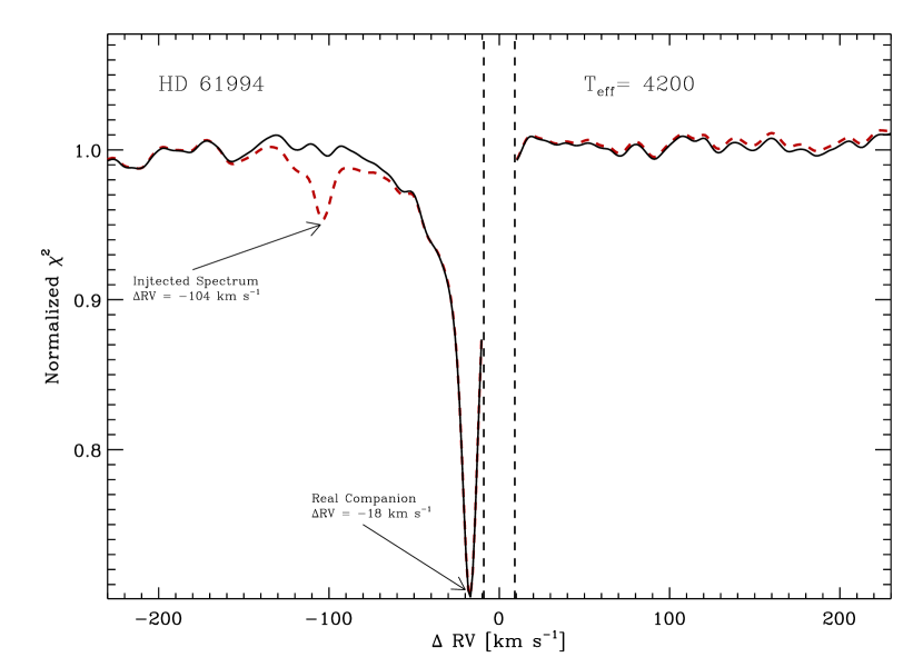
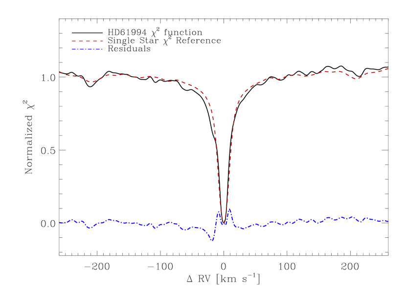
4.2.5 HD 61994
HD 61994 is a double-lined spectroscopic binary with a period of 552.8 days (Strassmeier et al. 2012). When the spectrum was taken, the relative radial velocity for the two stars was only +18 , an interesting example for cases where the relative radial velocity is low and the secondary star is something other than an M-dwarf. Furthermore, the companion is faint - the visible brightness ratio for the two stars is only 0.069 (Strassmeier et al. 2012).
The primary deviates slightly from the characteristic single-star function at RV -20 , shown in Figure 19. However, more convincing evidence for the presence of a secondary star comes from the residual function shown in Figure 9, indicating a secondary star at RV = 16 . Its residual minimum distribution function sets the secondary star at 4200 650 K. Within the uncertainty limit, this agrees with the Strassmeier et al. (2012) value of = 4775 150 K. The calculated flux ratio, = 0.055 0.022, also matches the flux ratio of = 0.069, quoted by Strassmeier et al. (2012).
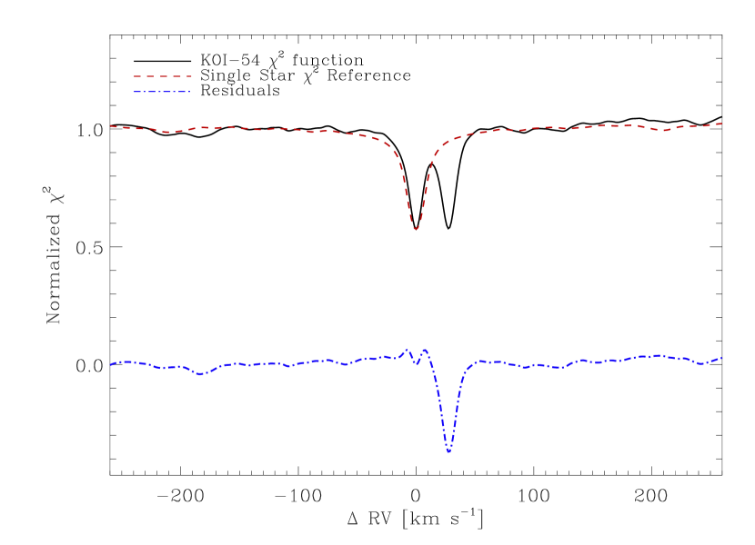
4.2.6 KOI-54
KOI-54 is a non-eclipsing, SB2 binary system. The two stars are in an almost face-on, highly eccentric orbit (Welsh et al. 2011).
This example shows the ability to detect the presence of both stars even when their effective temperatures are outside the range of our library and above the highest SpecMatch library spectrum temperature used to construct the residual panels. The primary star has a temperature = 8800200 K, and the companion lags behind this value only slightly with = 8500200 K (Welsh et al. 2011). This is over 2000 K higher than any of our library spectra.
Nonetheless, we are able to see the minimum in the function shown in Figure 20 due to each of the two stars, as well as detect a clear minimum indicating the presence of the companion after the primary star was subtracted, as seen in Figure 21. We don’t state the parameters obtained for KOI-54 system, since they are incorrect due to the large discrepancy between the stellar spectra for the KOI-54 stars and the available library spectra; more on this issue is explained in Section 6.2.
4.2.7 HD 16702
HD 16702 is identified as a binary star in Díaz et al. (2012), with the mass ratio for the companion and the primary star is = 0.350.41 (Díaz et al. 2012). We detect a secondary star at = 5 , with an estimated = 3500 250 K and contributing 1.06% of the total flux, as shown in Figures 22 and 23.
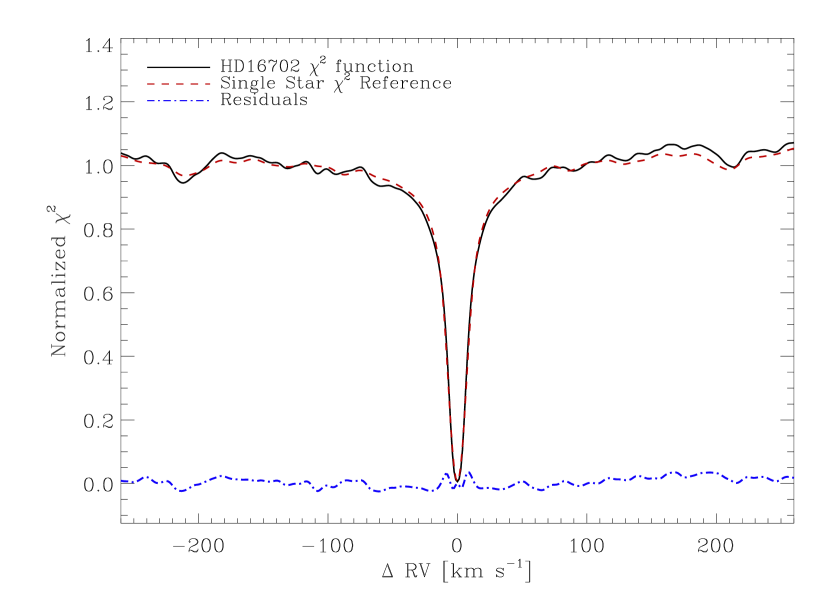
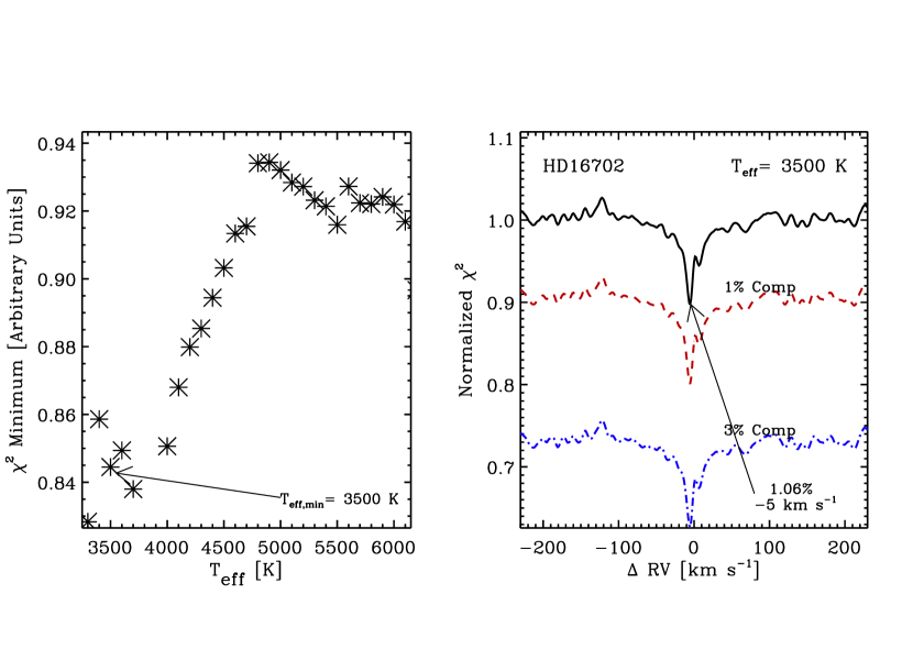
Since the only known companion parameter is its mass, we performed some analysis to confirm that our detection agrees with Díaz et al. (2012) value of 0.40 0.05 . Since the spectrum was taken when the velocity of both stars was almost exclusively along the line of sight, we can predict the mass of the companion based on their radial velocity separation. Using 9 precise RV measurements (Marcy & Butler 1992), we determine the primary star velocity relative to the center of mass of the binary system to be at its maximum at the time of observation, = -2.2 . Using the primary mass of 0.98 (Díaz et al. 2012), and of 5 , as determined by our algorithm, we predict the mass ratio = 0.30. This indicates a companion mass of 0.3 , only slightly below the Díaz et al. (2012) value. Using known calibrations, both the flux ratio of 0.01 and the companion temperature of 3500 K are consistent with a star whose mass is approximately 0.4 .
5. Application: 1160 Kepler Objects
We have carried out a spectroscopic survey of the 1160 Kepler Objects of Interest (KOI) that are brighter than Kepler magnitude of 14.2, announced as of September 2013 by the Kepler Project and listed in the Exoplanet Archive111http://exoplanetarchive.ipac.caltech.edu. A complete description of the 1160 KOIs and our spectra of them are provided by Howard et al. (2014, in prep). We obtained a Keck-HIRES spectrum with a SNR of 45 per pixel and a resolution of R = 60,000 from 3800 to 8000 for each one. All spectra are available to the public on the Keck Observatory Archive.
In Table 9 we identify the KOIs where a secondary star was detected by our algorithm here, and provide the deduced parameters of both the primary star and the companion. The uncertainties are determined using Table 5, which were computed using the injection-recovery tests. Companion plots for identified KOI binary systems are shown in Appendix, Figures 24 through 84.
Out of 1160 KOIs, 60 KOIs show clear evidence of companion stars using our spectroscopic algorithm. Additionally, we report three detections that were marginal. Among all of them, we found 41 KOIs that have one planetary candidate (one validated as a planet), three KOIs that have two planetary candidates, and one KOI with three planetary candidates. In addition, 15 of the 60 KOIs had been marked as false positives in the Exoplanet Archive.
Of course, these spectroscopic detections of secondary stars do not necessarily imply that the planet candidate is false. Instead, each detection merely indicates that there is either a background star or a bound companion to the target KOI. In either case, the transit lightcurve could be caused by a planet transiting the primary star, albeit with a diluted light curve, or an orbiting object that blocks the light of the secondary star, either bound or background.
The relative brightness of the secondary and the primary star can be used to compute the dilution factor of the Kepler light curves. Our wavelength domain encompasses approximately the V and R bandpasses of the classical photometry, and the relative brightness can thus be converted to the corresponding value in the Kepler bandpass, and used to determine a more accurate radius for the planet.
Some of the KOIs had secondary stars hotter than the primary star, but contributed only a few percent of the total flux. There are three possible explanations for such cases. First, the primary star might actually have already evolved off main sequence, and became a red giant. In this case, it would be possible that it is in fact cooler than the secondary, if the secondary is still on main sequence. Second possible explanation is that only a fraction of the flux from the secondary actually entered the spectrometer slit, thus not all of the flux from the secondary star is collected by the spectrometer. A third alternative is that the secondary star is simply a background star much further away.
5.1. KOI Companion Detections
This section is intended to be used in conjunction with the list of detected companions in Table 9, providing additional information relevant for selected KOIs. We also list the number of confirmed planets, planetary candidates, or indicate whether the KOI was identified as a false positive.
5.1.1 Confirmed Planets
KOI-1361
Also known as Kepler-61, it has one confirmed planet (Ballard et al. 2013). We determined the primary star temperature to be = 4265 145, which is 100 K larger compared to Ballard et al. (2013). We identified an even cooler companion, with = 3600 130 K, at a radial velocity of + 40 relative to the primary star. Ballard et al. (2013) reports a companion 0.94” north of the primary star, detected using adaptive optics. The magnitude difference between the primary star and the companion, as reported by Ballard et al. (2013), is 2.98 mag in Kepler bandpass. This corresponds to the flux ratio of = 0.064, which is only slightly above the value deduced by our algorithm, = 0.022 0.003. Some of this difference can be attributed to the difference in the Kepler bandpass regions as compared to the regions used in our algorithm. It is also possible that the spectrometer slit was not necessarily aligned to capture all of the light from the companion, thus the flux ratio is correspondingly lower.
5.2. Secondary Stars to KOIs with Three Planet Candidates
KOI-2311
Due to a low RV separation of +11 , the flux ratio of 0.276 0.069 is a lower limit. The final secondary star plot is shown in Figure 49.
5.2.1 Secondary Stars to KOIs with Two Planet Candidates
KOI-5
The observed RV trend indicates a possibility of a stellar companion (Wang et al. 2014). Low of +11 might have caused some of the secondary absorption lines to be subtracted away with the primary star, thus the quoted flux ratio of 0.066 0.020 is a lower limit rather than an actual value. We analyzed several different observations of the same star, and the RV separation varied with observation time. This indicates that the secondary and the primary star form a bound system. The final companion plot is shown in Figure 24.
KOI-354
Detection of the secondary star to the KOI-354 is marginal, thus we don’t list in in the Table 9. The system consists of a 5936 102 primary star (cfop.ipac.caltech.edu) and an M-dwarf secondary with = 3500 250 K. The secondary star has a low relative radial velocity of +11 , and thus the flux ratio of = 0.005 001 is a lower limit. The secondary star plot for KOI-354 is shown in Figure 27.
KOI-1613
Due to a low RV separation of +10 , the flux ratio of 0.044 0.013 is a lower limit. Law et al. (2014) detected a secondary star at a separation of 0.22”, 1.3 magnitudes fainter than the primary star. 1.3 magnitude difference indicates a flux ratio of 0.30, much higher than our lower limit. Since they observed the system in a different bandpass (roughly 7000-8000), this flux discrepancy can be somewhat due to a different flux ratios in different wavelength regions. However, we suspect that most of the discrepancy can be attributed to the low separation of the two stars of similar spectral types. At 10 = , the two sets of absorption lines are barely resolved, and most likely a large fraction of the secondary star was subtracted away together with the primary, leaving only a weak signal in the residuals. The final secondary star plot is shown in Figure 41.
KOI-2059
M-dwarf secondary star has a small RV separation of only +5 , making the flux ratio of 0.016 0.008 a lower limit. Nevertheless, due to a significantly different secondary spectral type of the secondary compared to the primary with of 5996 103 K (cfop.ipac.caltech.edu), we don’t expect the actual flux ratio to deviate significantly from this lower limit. Using AO, a companion was detected at a separation of 0.38”, 1.1 magnitude fainter (Law et al. 2014). A magnitude difference of 1.1 predicts the flux ratio of about 0.36, which is again larger than the ratio predicted by our algorithm. Again, since the Law et al. (2014) observation was made in the near-infrared region, where the flux of the M-dwarfs is considerably larger, we do expect that the flux ratio of an M-dwarf and a 5000 K primary star is higher as compared to the ratio in the V and R bandpasses. Therefore, our flux ratio is still consistent with the Law et al. (2014) value, especially when accounting for the fact that the ratio predicted by our algorithm as a lower limit. The final secondary star plot is shown in Figure 46.
5.2.2 Companions to KOIs with One Planet Candidate
Here we provide notes about selected KOIs that have one planet candidate, and an indication from our spectroscopic analysis of a secondary set of absorption lines in the spectrum. A complete listing of all such detections is in Table 9.
KOI-151
Due to a low separation of +14 , the flux ratio of 0.012 0.006 represents a lower limit for KOI-151 and its secondary star. The final secondary star plot is shown in Figure 25.
KOI-219
Both the flux ratio of 0.330 0.033 as well as the secondary star of 6000 100 K represent lower limits due to a restricted library range and low RV separation, respectively. The final secondary star plot is shown in Figure 26.
KOI-652
KOI-652 is at least a triple star system, with a possible marginal detection of the fourth star. All three companions are M-dwarfs, each contributing only a few percent to the total flux. The final companion plot is shown in Figure 28. In Table 9, we don’t list the faintest companion at 44 , as its detection is only marginal.
KOI-698
This system is analyzed in Santerne et al. (2012). Assuming a main sequence companion, our estimate for the secondary star of 4800 600 K indicates a secondary mass of 0.7 - 0.8 , which is below the predicted value of 1.1 0.1 by Santerne et al. (2012). The final secondary star plot is shown in Figure 29.
KOI-716
The detection of KOI-716 is marginal, and we don’t include it in the Table 9. KOI-716 secondary star is extremely faint and at the threshold of detection, with a flux ratio of = 0.004 0.001. The primary star is has a = 6096 150 K (cfop.ipac.caltech.edu), and the secondary star is an M-dwarf with = 3500 250 K. Due to a relatively low RV separation of +18 , the flux ratio might be underestimated, yet we don’t expect the secondary star contribution to be larger than 1% of the total flux. KOI-716 has 1 planetary candidate, and the secondary star plot is shown in Figure 30.
KOI-984
AO imaging of KOI-984 revealed a companion of approximately equal magnitude 1.5 arcseconds apart (Law et al. 2014). Our algorithm, however, detects a marginal secondary star at = +33 with = 3500 150 K, contributing less than 1% to the total flux. This suggests that only a small fraction of the light from secondary star star actually entered the slit, and while we can confirm the possibility of the companion, its estimated parameters are highly inaccurate. The final secondary star plot is shown in Figure 32. Since the detection is marginal, we don’t list it in Table 9.
KOI-1020
KOI-1137
Despite low RV separation of +11 , the two stars are of sufficiently distinct spectral types that we don’t expect the flux ratio to be significantly higher than the calculated lower limit of 0.020 0.004. The final secondary star plot is shown in Figure 35.
KOI-1452
The primary star has = 7172 211 K (cfop.ipac.caltech.edu), which is outside our library range. While the binarity of the spectrum is clear, the parameters for the secondary star cannot be determined accurately enough to be published. This is mostly due to a high rotational broadening of the secondary absorption lines, indicating a secondary star with a spectral type outside the range of our SpecMatch library. The final secondary star plot is shown in Figure 40.
KOI-1784
Due to a low RV separation of 13 , the flux ratio of 0.192 0.058 represents a lower limit. The final secondary star plot is shown in Figure 44.
KOI-2075
The secondary star is faint, contributing less than 1% to the total flux. While the flux ratio of 0.008 0.004 is a lower limit due to a low RV separation of 13 , we don’t expect that a large fraction of the secondary absorption lines got subtracted away together with the primary star, as the two spectral types differ significantly from each other. The final secondary star plot is shown in Figure 47.
KOI-2215
This is a triple-lined spectrum, with both secondary and tertiary stars clearly detectable. Both additional stars are treated separately, but the uncertainties on the parameters might be slightly higher due to the blending of spectral lines as the spectral types of all three stars are relatively similar. The flux ratio for the third star of 0.155 0.047 is a lower limit due to a low RV separation of 15 . The final secondary star plot is shown in Figure 48.
KOI-2457
The primary star effective temperature of 6728 155 (cfop.ipac.caltech.edu), exceeds our temperature range of the SpecMatch library. This hinders our ability to determine accurate parameters for the secondary star at a low separation of +14 . Nevertheless, our analysis indicates a secondary star with a lower limit flux ratio of 0.076 0.023. The final secondary star plot is shown in Figure 50.
KOI-3471
The spectrum of KOI-3471 contains four stars, all but one of comparable brightness. We provide estimates for the parameters for each of the constituent stars, but we expect larger errors due to significant blending of their spectral lines. Since all of the stars are contained within less than 80 , we expect that the temperatures as well as the flux ratios for additional stars are affected by the presence of the other all stars. The final plot is shown in Figure 64.
KOI-3573
Low RV separation of 15 together with similar spectral types of the two stars suggest that the actual flux ratio is probably higher than the calculated lower limit of 0.109 0.033. As the two sets of absorption lines overlap slightly, it is likely that a fraction of the secondary absorptions lines got subtracted away together with the primary star, thus making the secondary star appear fainter. The final secondary star plot is shown in Figure 70.
KOI-3583
The secondary star minimum is significantly broadened, indicating rotational broadening of secondary star absorption lines. Thus, despite the RV separation of 23 , there is a possibility for the blending of the two sets of absorption lines, and the calculated flux ratio of 0.109 0.033 is a lower limit. The final secondary star plot is shown in Figure 71.
KOI-3606
Both the secondary and the primary minimum are broadened, indicating a significant rotational broadening of the spectral lines. As this is characteristic of hot stars, we assume that the actual for the secondary star is above the quoted lower limit of 6000 100 K. The final secondary star plot is shown in Figure 74.
KOI-3721
The spectrum of KOI-3721 contained three sets of absorption lines, with the faintest star contributing only 1% to the total flux. Brighter secondary star is broad, indicating significant rotational broadening. This is consistent with the estimate of the secondary star above 6000 100 K. The final plot is shown in Figure 75.
KOI-3782
The calculated flux ratio is a lower limit due to a low RV separation of 7 , but we don’t expect a significant deviation from the stated flux ratio due to significantly different spectral types of the two stars. The final secondary star plot is shown in Figure 76.
KOI-4713
Due to similar spectral types of the two stars as well as the small RV separation of 15, the calculated flux ratio of 0.344 103 is a lower limit. The final secondary star plot is shown in Figure 83.
KOI-4871
Despite the RV separation of 23 , we state the flux ratio of 0.012 0.003 as the lower limit due to the similarity of the primary and secondary star spectral type. This similarity allows for a chance of overlap of some of the absorption lines, and some of the secondary absorption lines might have been subtracted away with the primary star. The final secondary star plot is shown in Figure 84.
5.2.3 Confirmed False Positives
KOI-1152
KOI-1152 has a known companion, previously detected using AO (Law et al. 2014). The planet candidate identified as a false positive (cfop.ipac.caltech.edu). We analyzed several different observations of the same star, and the RV separation varied with different observation times. This indicates that the secondary and the primary star form a bound system. The final secondary star plot is shown in Figure 36.
KOI-3000
Flux ratio of 0.055 0.019 is a lower limit rather than an actual value due to a low RV separation of +10 . Nevertheless, the two stars have sufficiently different spectral types that we do not expect significant departure from the stated flux ratio. The final secondary plot is shown in Figure 55.
KOI-3035
Despite moderate RV separation of +20 both sets of spectral lines are rotationally broadened, causing the two sets of absorption lines to overlap slightly. Therefore, the flux ratio of 0.212 0.064 is a lower limit rather than an actual value. The final secondary star plot is shown in Figure 57.
KOI-3162
Flux ratio of 0.553 0.166 is a lower limit due to a low RV separation of 13 . The final secondary star plot is shown in Figure 59.
KOI-3216
Flux ratio of 0.326 0.033 is a lower limit due to a low RV separation of +13 . The final secondary star plot is shown in Figure 60.
KOI-4355
The secondary star to KOI-4355 exhibited a broad minimum, indicating significant rotational broadening. Due to shallower spectral lines, the uncertainties on the secondary star parameters might be somewhat larger. The final secondary star plot is shown in Figure 81.
KOI-4457
The calculated flux ratio of 0.012 0.003 is a lower limit due to a low RV separation of 15 , but we don’t expect significant deviation from the stated value due to significantly different spectral types of the two stars. The final secondary star plot is shown in Figure 82.
6. Limitations
6.1. Relative Radial Velocity for the Secondary Star
Our code cannot detect secondary stars with 10 , with the exception of M-dwarfs. For bound systems consisting of two solar type stars, this corresponds to the physical separation of at most 5 AU, assuming the orbital plane is viewed edge-on and that the spectrum was taken when the two stars were coming directly towards/away from us. On the other hand, if the phase of the two stars is such that their momentary velocity is close to tangential, our code will not be able to detect the presence of the secondary star, regardless of their relative brightness. Somewhat less strictly, we are also limited to the orbits with periods larger than 2.5 days, as the maximum detectable Doppler shift for the secondary star is at 200 . This limit is determined assuming that the two stars in the binary system are solar type, that the spectrum was taken when the two stars were coming directly towards/away from us, and that the orbit is viewed edge-on. Shorter orbital periods can thus be detected for binaries with lower mass companions, for orbits viewed at an angle, or when the spectrum was taken at a different orbital phase.
For both bound companions and background secondary stars, whenever the spectral types of the two stars are similar and their relative radial velocity low (20 , with the exact number depending upon the amount of the absorption line broadening in the spectrum), there is a possibility that some of the absorption lines of the secondary spectrum get subtracted away together with the primary star. In those cases, the flux of the secondary star is somewhat underestimated, and its parameters carry somewhat larger uncertainties.
6.2. Effective Temperature
The SpecMatch library used for our algorithm contains stars with from 3200 K to 6550 K. For detecting the secondary star, the range is slightly narrower, ranging from 3300 K to 6100 K. This is due to the fact that we only construct the median library spectrum for a particular 100 K range when there are at least three different SpecMatch spectra within that range. For any primary star with outside the SpecMatch library range, the fit will not be exact, and the subtraction will be imperfect - this decreases the detectability of the secondary stars with . Furthermore, for any secondary star with much lower than 3300 K or much higher than 6100 K we cannot accurately estimate the percentage flux as the injected spectrum cannot match the actual secondary star spectrum. Due to these reasons, deduced and flux contribution for stars outside the SpecMatch parameter range carry larger uncertainties. Nevertheless the binarity of the spectrum can still be established with a sufficient degree of certainty (see KOI-54 example in Section 4.2.6).
Since we cannot extrapolate the minima distribution function to temperatures lower than 3300 K, we cannot predict whether a secondary star whose effective temperature is estimated at 3300 K is actually cooler than this limiting temperature. Thus, the 3300 K secondary star is always more of an upper limit than an actual value. Similarly, we cannot extrapolate the behavior of the minima distribution to effective temperatures higher than 6000 K, and any 6100 K estimated secondary star is a thus a lower limit rather than the actual estimate.
6.3. Rotational Broadening
Rotational broadening does not pose a major challenge to the identification of the primary star, as we artificially broaden the library spectrum’s absorption lines to match the amount of broadening present in the spectrum. We can fit and subtract the primary absorption lines successfully regardless of the star’s rotation. For the secondary star, however, any significant broadening of absorption lines impairs our ability to detect it. As the lines become broader, they become shallower, thus less distinct from the noise. This also causes a less sharp and distinct residual minimum, that cannot be as easily distinguished from accidental alignments.
For cases where the secondary star has a significant rotational broadening but is sufficiently bright to enable detection, the estimated secondary temperature and its flux contribution become more uncertain. Since we do not artificially broaden the lines of the median library spectra used for the search of the secondary star, even the spectrum with matching that of the actual secondary star is a poor match. Thus, since none of the median library spectra match the secondary star well, the differences in the minima are smaller among the values for the median library spectra, and the residual minimum distribution’s minimum is harder to identify correctly. Furthermore, shallower absorption lines cause the underestimation of the flux contribution, and the flux ratio for the two stars is underestimated as well.
6.4. Fractional Flux Contribution from the Secondary Star
For the secondary star to be detectable, its fractional contribution most often needs to reach a value that is at least one half of the noise; for example, a 1% flux from the secondary star for a spectrum with 2% can be detected. This brings the SNR of the residuals after the subtraction of the primary star to 0.5. The exact value also depends on the spectral differences between the two stars, as well as their relative radial velocity.
At the other end, secondary stars with fractional contributions comparable to that of their primary stars pose a challenge as well. While those stars are easily detectable, the determination of the properties for the secondary star is limited by the pollution of one set of absorption lines by the other. This effect is especially apparent when their relative radial velocity is low, with one set of lines encroaching on the other significantly. In those cases, both the primary star fit as well as the secondary star parameters suffer by this mutual pollution of their respective absorption lines. Since some of the secondary absorption lines get subtracted away together with the primary star, this also causes the calculated flux ratio for the two stars to be below the true value.
7. Conclusion
Using the algorithm described in this paper we were able to detect secondary stars in the Keck-HIRES spectra that contributed as low as 1% of the total flux in the spectrum with a 2% Poisson noise. These secondary stars can be angularly separated from the primary star by at most 0.43” to 1.5”, depending on the orientation of the aperture slit. For detection, the relative radial velocity for the two stars needs to exceed 10 , except for the case of the G-type primary star and an M-dwarf. For G-M pairs, there is no restriction on the radial velocity separation for the two stars, given that the two sets of absorption lines are not overlapping exactly; for these, we were able to detect secondaries as faint as 0.5% relative to the primary star in a spectrum with a 2% Poisson noise. Our results suggests the detectability threshold SNR for the secondary star of 0.5 for any spectral type combination of the two stars, and 0.25 for M-dwarf secondaries to G-type primary stars.
For cases where the secondary star is detected, its effective temperature and the fractional flux contribution can be determined. The uncertainties in the derived parameters depend on the relative brightness of the secondary star as well as on the spectral types of the two stars in the spectrum. These values are summarized in Table 5. For the cases of non-detections, we place an upper limit for the brightness of any potential hidden companions.
Currently, we are limited to stars with the effective temperature above 3300 K and below 6500 K; for the stars outsides this temperature range, the presence of the sufficiently bright secondary star can still be evaluated, but the derived parameters carry larger uncertainties. The parameter errors also increase when the two stars have comparable flux contributions, or when their spectral types are similar. Our results are most accurate for the cases where the relative radial velocity of the two stars exceeds 10 , both stars have between 3000 K and 6000 K, and the secondary star contributes less than 20% of the total flux for the system. The recovery rate for a given radial velocity separation and relative brightness of the secondary star is the highest for M-dwarfs, given that the primary stars is of a different spectral type.
This spectroscopic algorithm can be useful for transiting planets towards recognizing multiple potential host stars for the planet and for computing photometric dilution in the analysis of the planet. As an application of the algorithm, we analyzed 1160 Kepler objects of interest and found and evidence of at least one additional star in 63 KOIs. A secondary star does not imply that the planet is false, but merely indicates that there is another star present angularly close to the primary star, either bound or background. Our estimate of the fractional flux contribution from the secondary star for each of these 63 KOIs can be used to compute the dilution factor for their Kepler light curves, and help to determine a more accurate radius of the planet.
Acknowledgments
We thank John Johnson for the CalTech Keck Telescope time to obtain many of the spectra of the KOIs. We also thank John Brewer and Debra Fischer for their preliminary estimates of the stellar parameters for the Specmatch library stars, as their parameters are an improvement over the values in Valenti & Fischer (2005), with a published paper in preparation. G. Marcy, the Alberts Chair at UC Berkeley, would like to thank the Marilyn and Watson Alberts for funding that made this research possible. We also thank the John Templeton Foundation and NASA grant NNX11AK04A for funding this research. We thank the government of the Republic of Slovenia and its Slovene Human Resources and Scholarship Fund and its Ad futura programme that helps fund R. Kolbl.
Kepler was competitively selected as the tenth NASA Discovery mission. Funding for this mission is provided by the NASA Science Mission Directorate. Some of the data presented herein were obtained at the W. M. Keck Observatory, which is operated as a scientific partnership among the California Institute of Technology, the University of California, and the National Aeronautics and Space Administration. The Keck Observatory was made possible by the generous financial support of the W. M. Keck Foundation.
The authors would like to thank the many people who gave so generously of their time to make NASA Kepler Mission a success. All spectra used in this paper are available at the Keck Observatory Archive. All Kepler data products are available to the public at the Mikulski Archive for Space Telescopes http://stdatu.stsci.edu/kepler and the spectra and their products are made available at the NExSci Exoplanet Archive and its CFOP website: http://exoplanetarchive.ipac.caltech.edu We thank the many observers who contributed to the measurements reported here. We gratefully acknowledge the efforts and dedication of the Keck Observatory staff, especially Scott Dahm, Hien Tran, and Grant Hill for support of HIRES and Greg Wirth for support of remote observing. This work made use of the SIMBAD database (operated at CDS, Strasbourg, France) and NASA’s Astrophysics Data System Bibliographic Services. This research has made use of the NASA Exoplanet Archive, which is operated by the California Institute of Technology, under contract with the National Aeronautics and Space Administration under the Exoplanet Exploration Program. Finally, the authors wish to extend special thanks to those of Hawai‘ian ancestry on whose sacred mountain of Mauna Kea we are privileged to be guests. Without their generous hospitality, the Keck observations presented herein would not have been possible.
| Name | [K] | log [mag] | M [] | R [] | [mag] | Source |
|---|---|---|---|---|---|---|
| GL 273 | 3293 | 0.29 | 0.31 | 0.17 | Rojas-Ayala et al. (2012) | |
| GL 687 | 3395 | 0.40 | 0.40 | 0.09 | Rojas-Ayala et al. (2012) | |
| GL 408 | 3526 | 0.38 | 0.38 | 0.09 | Rojas-Ayala et al. (2012) | |
| GL 250B | 3569 | 0.45 | 0.43 | 0.01 | Rojas-Ayala et al. (2012) | |
| GL 686 | 3693 | 0.45 | 0.43 | 0.28 | Rojas-Ayala et al. (2012) | |
| HIP 24284 | 3992 | 4.88 | 0.41 | 0.36 | 0.49 | SME Analysis |
| HIP 41689 | 4088 | 4.83 | 0.47 | 0.39 | 0.45 | SME Analysis |
| HD 217357 | 4200 | 4.74 | 0.55 | 0.46 | 0.17 | SME Analysis |
| HIP 105341 | 4298 | 4.72 | 0.58 | 0.55 | 0.05 | SME Analysis |
| HIP 99205 | 4397 | 4.70 | 0.63 | 0.59 | 0.18 | SME Analysis |
| HIP 36551 | 4501 | 4.69 | 0.65 | 0.60 | 0.30 | SME Analysis |
| HIP 103650 | 4602 | 4.68 | 0.69 | 0.63 | 0.04 | SME Analysis |
| HIP 63762 | 4701 | 4.62 | 0.74 | 0.69 | 0.09 | SME Analysis |
| HD 220221 | 4797 | 4.58 | 0.79 | 0.75 | 0.18 | SME Analysis |
| HD 51866 | 4906 | 4.59 | 0.80 | 0.75 | 0.13 | SME Analysis |
| HD 23356 | 4988 | 4.60 | 0.78 | 0.73 | 0.04 | SME Analysis |
| HD 216520 | 5097 | 4.55 | 0.78 | 0.77 | 0.19 | SME Analysis |
| HD 205855 | 5204 | 4.53 | 0.86 | 0.83 | 0.05 | SME Analysis |
| HD 75732 | 5295 | 4.49 | 0.97 | 0.92 | 0.39 | SME Analysis |
| HD 58727 | 5399 | 4.52 | 0.97 | 0.90 | 0.24 | SME Analysis |
| HD 147750 | 5496 | 4.52 | 0.90 | 0.85 | 0.11 | SME Analysis |
| HD 20619 | 5600 | 4.42 | 0.87 | 0.94 | 0.25 | SME Analysis |
| HD 12661 | 5699 | 4.38 | 1.09 | 1.11 | 0.35 | SME Analysis |
| HD 148284 | 5799 | 4.39 | 1.11 | 1.10 | 0.29 | SME Analysis |
| HD 205351 | 5896 | 4.29 | 1.11 | 1.23 | 0.09 | SME Analysis |
| HD 27859 | 5997 | 4.41 | 1.14 | 1.09 | 0.14 | SME Analysis |
| HD 48682 | 6104 | 4.36 | 1.18 | 1.18 | 0.11 | SME Analysis |
Note. — No precise log values are available for M-dwarfs.
| Primary | Secondary [K] | |||||
|---|---|---|---|---|---|---|
| 3500 | 4000 | 4500 | 5000 | 5500 | 6000 | |
| 1% Secondary | ||||||
| 3500 | 50% | 40% | 40% | 60% | 60% | 60% |
| 4000 | 70% | 70% | 70% | 70% | 70% | 70% |
| 4500 | 80% | 70% | 80% | 80% | 70% | 70% |
| 5000 | 80% | 80% | 70% | 70% | 80% | 70% |
| 5500 | 100% | 90% | 90% | 100% | 100% | 80% |
| 6000 | 80% | 70% | 80% | 70% | 80% | 80% |
| 3% Secondary | ||||||
| 3500 | 100% | 90% | 100% | 100% | 100% | 100% |
| 4000 | 90% | 90% | 90% | 90% | 90% | 90% |
| 4500 | 100% | 100% | 100% | 100% | 100% | 90% |
| 5000 | 90% | 100% | 100% | 100% | 90% | 90% |
| 5500 | 100% | 100% | 100% | 100% | 100% | 100% |
| 6000 | 90% | 100% | 100% | 100% | 90% | 90% |
| 10% Secondary | ||||||
| 3500 | 100% | 100% | 100% | 100% | 100% | 100% |
| 4000 | 100% | 100% | 100% | 100% | 100% | 100% |
| 4500 | 100% | 100% | 100% | 100% | 100% | 100% |
| 5000 | 100% | 100% | 100% | 100% | 100% | 100% |
| 5500 | 100% | 100% | 100% | 100% | 100% | 100% |
| 6000 | 100% | 100% | 100% | 100% | 100% | 100% |
| Primary [K] | Secondary [K] | |||||
|---|---|---|---|---|---|---|
| 3500 | 4000 | 4500 | 5000 | 5500 | 6000 | |
| 1% Secondary | ||||||
| 3500 | 75 70 | 565 200 | 30 695 | 245 415 | 45 465 | 500 465 |
| 4000 | 45 155 | 175 440 | 55 530 | 470 440 | 230 320 | 180 330 |
| 4500 | 0 125 | 195 455 | 80 220 | 285 260 | 355 70 | 115 180 |
| 5000 | 85 155 | 500 125 | 230 135 | 205 230 | 14- 390 | 50 20 |
| 5500 | 5 155 | 230 440 | 140 235 | 260 235 | 375 95 | 60 25 |
| 6000 | 85 155 | 500 125 | 230 125 | 205 230 | 140 390 | 50 20 |
| 3% Secondary | ||||||
| 3500 | 60 185 | 470 340 | 200 355 | 85 410 | 180 360 | 85 65 |
| 4000 | 5 130 | 380 420 | 195 325 | 80 480 | 255 440 | 205 450 |
| 4500 | 25 135 | 385 370 | 250 350 | 195 295 | 355 145 | 50 150 |
| 5000 | 0 135 | 80 370 | 250 250 | 210 385 | 225 435 | 330 495 |
| 5500 | 5 160 | 375 255 | 225 255 | 220 320 | 375 105 | 50 150 |
| 6000 | 0 135 | 80 375 | 250 250 | 210 370 | 205 435 | 330 495 |
| 10% Secondary | ||||||
| 3500 | 15 145 | 295 170 | 22 185 | 70 245 | 155 345 | 50 50 |
| 4000 | 5 130 | 250 120 | 50 220 | 15 275 | 230 280 | 50 50 |
| 4500 | 10 130 | 205 135 | 100 50 | 20 315 | 195 320 | 100 14 |
| 5000 | 0 150 | 205 85 | 25 150 | 30 255 | 145 245 | 20 50 |
| 5500 | 5 150 | 190 160 | 130 65 | 95 345 | 320 125 | 50 20 |
| 6000 | 0 150 | 300 80 | 150 100 | 30 255 | 145 245 | 40 50 |
| Primary [K] | Secondary [K] | |||||
|---|---|---|---|---|---|---|
| 3500 | 4000 | 4500 | 5000 | 5500 | 6000 | |
| 1% Secondary | ||||||
| 3500 | 0.25 0.10 | 0.28 0.89 | 0.03 0.33 | 0.30 0.24 | 0.21 0.29 | 0.15 0.34 |
| 4000 | 0.21 0.11 | 0.20 0.26 | 0.01 0.11 | 0.18 0.24 | 0.10 0.18 | 0.04 0.21 |
| 4500 | 0.10 0.26 | 0.11 0.26 | 0.07 0.12 | 0.25 0.34 | 0.16 0.11 | 0.14 0.16 |
| 5000 | 0.32 0.19 | 0.32 0.19 | 0.03 0.19 | 0.04 0.25 | 0.02 0.17 | 0.05 0.22 |
| 5500 | 0.15 0.18 | 0.11 0.26 | 0.11 0.17 | 0.12 0.20 | 0.23 0.31 | 0.07 0.14 |
| 6000 | 0.32 0.18 | 0.32 0.19 | 0.03 0.19 | 0.04 0.25 | 0.02 0.17 | 0.05 0.22 |
| 3% Secondary | ||||||
| 3500 | 0.34 0.90 | 0.67 0.45 | 0.00 0.40 | 0.21 0.66 | 0.34 0.70 | 0.35 0.74 |
| 4000 | 0.32 0.43 | 0.71 0.65 | 0.08 0.32 | 0.23 0.57 | 0.24 0.78 | 0.19 0.69 |
| 4500 | 0.38 0.43 | 0.62 0.50 | 0.07 0.69 | 0.25 0.50 | 0.31 0.52 | 0.02 0.34 |
| 5000 | 0.31 0.86 | 0.11 0.79 | 0.12 0.23 | 0.18 0.18 | 0.11 0.14 | 0.49 0.16 |
| 5500 | 0.25 0.49 | 0.67 0.49 | 0.21 0.38 | 0.18 0.42 | 0.45 0.53 | 0.04 0.29 |
| 6000 | 0.18 0.87 | 0.11 0.79 | 0.12 0.23 | 0.18 0.18 | 0.11 0.14 | 0.69 0.16 |
| 10% Secondary | ||||||
| 3500 | 1.17 1.34 | 3.09 1.21 | 0.35 1.85 | 0.06 2.25 | 2.63 2.50 | 1.17 1.42 |
| 4000 | 1.26 1.40 | 3.43 1.09 | 0.23 1.40 | 1.92 1.44 | 1.84 0.77 | 0.68 1.44 |
| 4500 | 1.32 1.55 | 2.95 0.77 | 0.12 1.05 | 1.26 0.83 | 1.97 1.08 | 1.07 1.97 |
| 5000 | 0.07 0.15 | 2.23 1.43 | 0.29 0.70 | 1.25 0.93 | 1.76 0.83 | 1.55 1.53 |
| 5500 | 0.55 1.56 | 2.00 1.00 | 0.84 0.78 | 1.71 0.41 | 1.71 0.53 | 0.47 0.50 |
| 6000 | 0.07 0.16 | 2.23 1.43 | 0.29 0.70 | 0.42 0.58 | 1.76 0.83 | 1.55 1.53 |
| Primary [K] | Secondary [K] | |||||||||||
|---|---|---|---|---|---|---|---|---|---|---|---|---|
| 3500 | 4000 | 4500 | 5000 | 5500 | 6000 | 3500 | 4000 | 4500 | 5000 | 5500 | 6000 | |
| Absolute Uncertainty, [K] | Relative Flux Ratio Uncertainty∗, | |||||||||||
| 1% Secondary | 1% Secondary | |||||||||||
| 3500 | 150 | 750 | 750 | 650 | 500 | 950 | 0.35 | 1.15 | 0.35 | 0.55 | 0.50 | 0.50 |
| 4000 | 200 | 600 | 600 | 900 | 550 | 500 | 0.30 | 0.45 | 0.10 | 0.40 | 0.30 | 0.25 |
| 4500 | 150 | 650 | 300 | 550 | 450 | 300 | 0.35 | 0.35 | 0.20 | 0.60 | 0.25 | 0.30 |
| 5000 | 250 | 650 | 350 | 450 | 400 | 100 | 0.50 | 0.50 | 0.20 | 0.30 | 0.20 | 0.30 |
| 5500 | 150 | 650 | 400 | 500 | 450 | 100 | 0.35 | 0.35 | 0.30 | 0.30 | 0.55 | 0.20 |
| 6000 | 250 | 650 | 350 | 450 | 550 | 100 | 0.50 | 0.50 | 0.20 | 0.30 | 0.20 | 0.25 |
| 3% Secondary | 3% Secondary | |||||||||||
| 3500 | 250 | 800 | 550 | 500 | 550 | 150 | 0.40 | 0.35 | 0.15 | 0.30 | 0.35 | 0.35 |
| 4000 | 150 | 800 | 500 | 550 | 700 | 650 | 0.25 | 0.45 | 0.15 | 0.25 | 0.35 | 0.30 |
| 4500 | 150 | 755 | 600 | 500 | 500 | 200 | 0.25 | 0.35 | 0.25 | 0.25 | 0.25 | 0.10 |
| 5000 | 150 | 450 | 500 | 600 | 650 | 850 | 0.40 | 0.30 | 0.10 | 0.10 | 0.10 | 0.20 |
| 5500 | 150 | 650 | 500 | 550 | 500 | 200 | 0.25 | 0.40 | 0.20 | 0.20 | 0.30 | 0.10 |
| 6000 | 150 | 450 | 500 | 600 | 650 | 850 | 0.35 | 0.30 | 0.10 | 0.10 | 0.10 | 0.30 |
| 10% Secondary | 10% Secondary | |||||||||||
| 3500 | 150 | 450 | 200 | 300 | 550 | 100 | 0.25 | 0.45 | 0.20 | 0.25 | 0.50 | 0.25 |
| 4000 | 150 | 350 | 250 | 350 | 500 | 100 | 0.25 | 0.45 | 0.15 | 0.35 | 0.25 | 0.20 |
| 4500 | 150 | 350 | 150 | 350 | 500 | 100 | 0.30 | 0.35 | 0.10 | 0.20 | 0.30 | 0.30 |
| 5000 | 150 | 300 | 200 | 300 | 400 | 100 | 0.10 | 0.35 | 0.10 | 0.20 | 0.25 | 0.30 |
| 5500 | 150 | 350 | 200 | 450 | 450 | 100 | 0.20 | 0.30 | 0.15 | 0.20 | 0.20 | 0.10 |
| 6000 | 150 | 400 | 250 | 300 | 400 | 100 | 0.05 | 0.35 | 0.10 | 0.10 | 0.25 | 0.30 |
Note. — ∗ The flux ratio of the secondary and the primary star is here denoted by , where .
| Secondary star | Recovery | [K] | Relative Flux [%] |
|---|---|---|---|
| Brightness | Rate | ||
| 1% | 40% | 35 170 | 0.01 0.22 |
| 3% | 90% | 10 130 | 1.18 0.56 |
| 5% | 90% | -5 140 | 2.05 0.70 |
| Parameter | Literature | Our Results | Discrepancy | Notes |
|---|---|---|---|---|
| KIC 10319590 | ||||
| 5518 200 | 5650 200 | / | MAST Online Catalogue | |
| Mass [] | 1.0 0.5 | MAST Online Catalogue | ||
| Radius [] | 0.9 0.5 | MAST Online Catalogue | ||
| log [mag] | 4.4 0.5 | 4.5 0.5 | / | MAST Online Catalogue |
| KIC 5473556 | ||||
| [K] | 5932 200 | 5800 200 | / | MAST Online Catalogue |
| Mass [] | 1.0 0.5 | MAST Online Catalogue | ||
| Radius [] | 0.9 0.5 | MAST Online Catalogue | ||
| log [mag] | 4.028 0.5 | 4.5 0.5 | / | MAST Online Catalogue |
| KIC 8572936 | ||||
| [K] | 5913 130 | 6000 200 | / | Welsh et al. (2011) |
| Mass [] | 1.0479 | 1.0 0.5 | / | Welsh et al. (2011) |
| Radius [] | 1.1618 | 1.1 0.5 | / | Welsh et al. (2011) |
| log [mag] | 4.32840.5 | 4.3 0.5 | / | Welsh et al. (2011) |
| KIC 9837578 | ||||
| [K] | 5606 150 | 5800 200 | / | Welsh et al. (2011) |
| Mass [] | 0.8877 | 0.9 0.5 | / | Welsh et al. (2011) |
| Radius [] | 1.0284 | 0.9 0.5 | / | Welsh et al. (2011) |
| log [mag] | 4.36230.5 | 4.5 0.5 | / | Welsh et al. (2011) |
| HD 61994 | ||||
| [K] | 5630 150 | 5750 200 | / | Strassmeier et al. (2012) |
| Mass [] | 1.1 0.5 | |||
| Radius [] | 1.3 0.5 | |||
| log [mag] | 4.13 0.11 | 4.2 0.5 | / | Strassmeier et al. (2012) |
| HD 16702 | ||||
| [K] | 5908 25 | 5800 200 | / | Díaz et al. (2012) |
| Mass [] | 0.98 0.04 | 1.1 0.5 | / | Díaz et al. (2012) |
| Radius [] | 1.0 0.5 | |||
| log [mag] | 4.46 0.03 | 4.4 0.5 | / | Díaz et al. (2012) |
| Parameter | Literature | Our Results | Discrepancy | Notes |
|---|---|---|---|---|
| KIC 10319590 | ||||
| [K] | 4300 500 | MAST Online Catalogue | ||
| Flux Ratio, | 0.036 0.007 | |||
| KIC 5473556 | ||||
| [K] | 6000 100 | MAST Online Catalogue | ||
| Flux Ratio, | 0.22 0.07 | |||
| KIC 8572936 | ||||
| [K] | 5867 130 | 6000 250 | / | Welsh et al. (2011) |
| Flux Ratio, | 0.8475 0.005 | 0.82 0.25 | / | Welsh et al. (2011) |
| KIC 9837578 | ||||
| [K] | 5202 100 | 5600 400 | / | Strassmeier et al. (2012) |
| Flux Ratio, | 0.3941 | 0.56 0.14 | 7% | Strassmeier et al. (2012) |
| HD 61994 | ||||
| [K] | 4775 150 | 4200 650 | / | Strassmeier et al. (2012) |
| Flux Ratio, | 0.069 | 0.055 0.022 | / | Strassmeier et al. (2012) |
| HD 16702 | ||||
| [K] | 3500 250 | |||
| Flux Ratio, | 0.016 0.008 | |||
| KOI | Primary Star | Companion Parameters | Planetary | ||
|---|---|---|---|---|---|
| [K] | [K] | Data∗ | |||
| 5 | 5753 75 | 5900 850 | 0.066 0.020 | +11 | 2 PC |
| 151 | 6276 163 | 3500 250 | 0.012 0.006 | +14 | 1 PC |
| 219 | 5513 184 | 6000 100 | 0.330 0.033 | +13 | 1 PC |
| 652 | 4700 128 | 3700 150 | 0.092 0.028 | +22 | 1 PC |
| 4000 350 | 0.020 0.007 | +46 | |||
| 3500 150 | 0.006 0.002 | 44 | |||
| 698 | 6120 196 | 4800 600 | 0.048 0.005 | +29 | 1 PC |
| 969 | 6224 186 | 6000 100 | 0.821 0.246 | 42 | 1 PC |
| 1020 | 6058 158 | 6000 100 | 0.292 0.088 | +39 | 1 PC |
| 1121 | 5671 156 | 6000 100 | 0.077 0.008 | 12 | 1 PC |
| 1137 | 5324 178 | 3600 150 | 0.020 0.004 | +11 | 1 PC |
| 1152 | 3806 50 | 4200 350 | 0.307 0.138 | +27 | 1 FP |
| 1227 | 5658 159 | 6000 100 | 0.821 0.082 | 123 | 1 PC |
| 1326 | 5378 173 | 6000 100 | 0.395 0.040 | +42 | 1 PC |
| 1361 | 4014 76 | 3600 200 | 0.022 0.007 | +40 | 1 CP |
| 1452 | 7172 211 | +81 | 1 PC | ||
| 1613 | 6044 117 | 6000 850 | 0.044 0.013 | +10 | 2 PC |
| 1645 | 5193 170 | 4500 200 | 0.287 0.029 | +55 | 1 PC |
| 1684 | 6428 134 | 6000 100 | 0.300 0.090 | 50 | 1 PC |
| 1784 | 5936 150 | 6000 100 | 0.192 0.058 | 13 | 1 PC |
| 1796 | 6065 205 | 3500 250 | 0.012 0.006 | +36 | 1 PC |
| 2059 | 4996 103 | 3600 250 | 0.016 0.008 | +5 | 2 PC |
| 2075 | 6403 159 | 3400 250 | 0.008 0.004 | 13 | 1 PC |
| 2215 | 5974 187 | 6000 100 | 0.185 0.056 | +32 | 1 PC |
| 6000 100 | 0.155 0.047 | 15 | |||
| 2311 | 5754 147 | 5600 400 | 0.276 0.069 | +11 | 3 PC |
| 2457 | 6728 155 | 6000 100 | 0.076 0.023 | +14 | 1 PC |
| 2787 | 6335 177 | 6000 100 | 0.222 0.067 | +16 | 1 FP |
| 2813 | 5143 164 | 6000 100 | 0.195 0.058 | +26 | 1 PC |
| 2867 | 4865 194 | 4700 200 | 0.389 0.136 | +44 | 1 PC |
| 2965 | 6468 159 | 6000 850 | 0.022 0.007 | +20 | 1 FP |
| 3000 | 5919 157 | 4100 450 | 0.055 0.019 | +10 | 1 FP |
| 3002 | 6060 152 | 6000 100 | 0.475 0.143 | 15 | 1 FP |
| 3035 | 6324 174 | 6000 100 | 0.212 0.064 | +18 | 1 FP |
| 3161 | 6790 195 | 6000 100 | 0.305 0.092 | 167 | 1 PC |
| 3162 | 6109 165 | 5900 100 | 0.553 0.166 | 13 | 1 FP |
| 3216 | 5615 166 | 6000 100 | 0.326 0.033 | +13 | 1 FP |
| 3231 | 6195 188 | 6000 100 | 0.175 0.053 | 22 | 1 FP |
| 3243 | 6348 146 | 6000 100 | 0.590 0.177 | +45 | 1 FP |
| 3415 | 5619 178 | 5600 200 | 0.786 0.157 | 71 | 1 PC |
| 3471 | 4847 118 | 4600 200 | 0.746 0.079 | 33 | 1 FP |
| 6000 100 | 0.202 0.061 | +26 | |||
| 4100 300 | 0.117 0.041 | 52 | |||
| 3506 | 6878 194 | 6000 100 | 0.206 0.062 | +137 | 1 PC |
| 3515 | 6395 155 | 6000 100 | 0.134 0.040 | +48 | 1 FP |
| 3527 | 5668 153 | 6000 100 | 0.880 0.264 | 16 | 1 PC |
| 3528 | 6061 200 | 6000 100 | 0.182 0.055 | +66 | 1 PC |
| 3557 | 6462 161 | 6000 100 | 0.393 0.118 | +55 | 1 FP |
| 3573 | 6403 158 | 6000 100 | 0.109 0.033 | 15 | 1 PC |
| 3583 | 7591 230 | 6000 100 | 0.109 0.033 | 23 | 1 PC |
| 3602 | 5940 157 | 6000 100 | 0.253 0.076 | +24 | 1 PC |
| 3605 | 5126 152 | 3600 150 | 0.044 0.018 | 57 | 1 PC |
| 3606 | 6570 177 | 6000 100 | 0.399 0.120 | +162 | 1 PC |
| 3721 | 6261 185 | 6000 100 | 0.143 0.043 | +51 | 1 PC |
| 4500 350 | 0.016 0.003 | 61 | |||
| 3782 | 5018 250 | 3400 135 | 0.022 0.011 | 7 | 1 PC |
| 3837 | 6540 181 | 4500 500 | 0.048 0.005 | +37 | 1 PC |
| 3853 | 5081 118 | 3400 250 | 0.009 0.001 | +22 | 1 PC |
| 3875 | 6022 198 | 6000 100 | 0.623 0.187 | 85 | 1 PC |
| 4345 | 5776 185 | 3600 250 | 0.012 0.006 | 48 | 1 PC |
| 4355 | 5780 | 6000 850 | 0.044 0.013 | 21 | 1 FP |
| 4457 | 6384 159 | 3600 250 | 0.012 0.006 | +11 | 1 FP |
| 4713 | 5780 | 6000 100 | 0.344 0.103 | 15 | 1 PC |
| 4871 | 6532 159 | 6000 100 | 0.012 0.003 | 23 | 1 PC |
Note. — Primary star and the associated uncertainties are taken from cfop.ipac.caltech.edu. Companion parameters are derived using our algorithm, and the uncertainties are determined using Table 5. Unless stated otherwise, we only have one observation of each spectrum listed above; therefore, we cannot test whether the secondary star is a part of the bound system or a background star.
∗From cfop.ipac.caltech.edu. PC - planet candidate, CP - confirmed planet, FP - false positive
Graphical supporting evidence for KOIs that showed an evidence of secondary star, listed in Table 9.
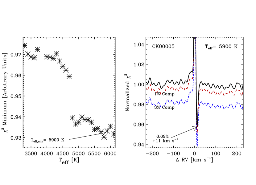
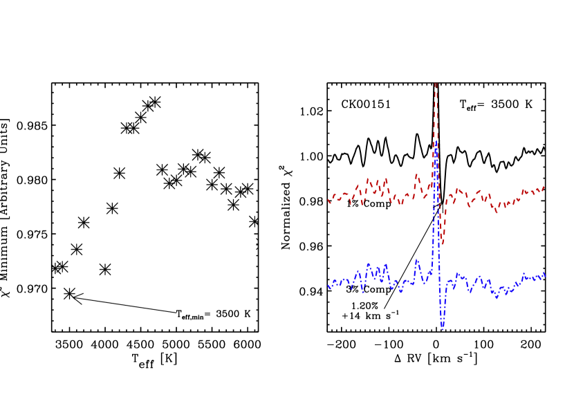
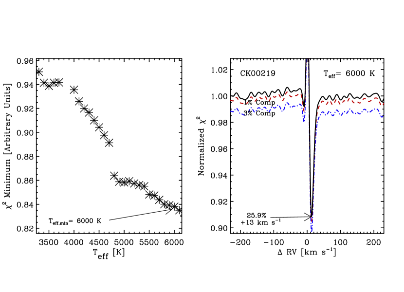
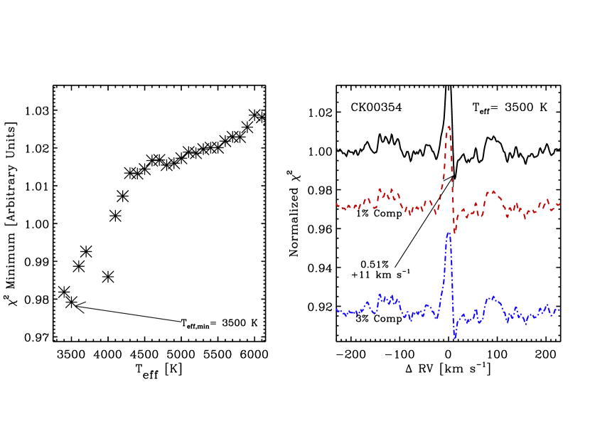
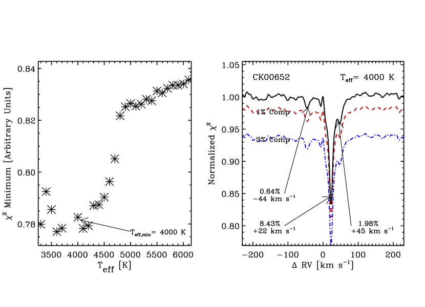
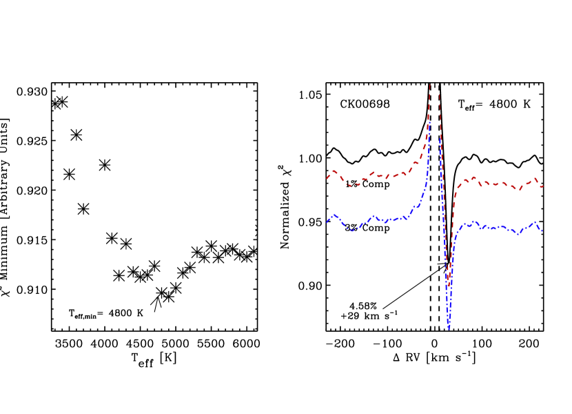
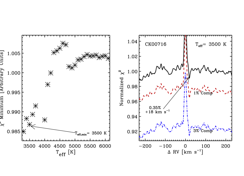
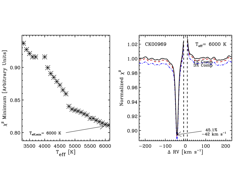
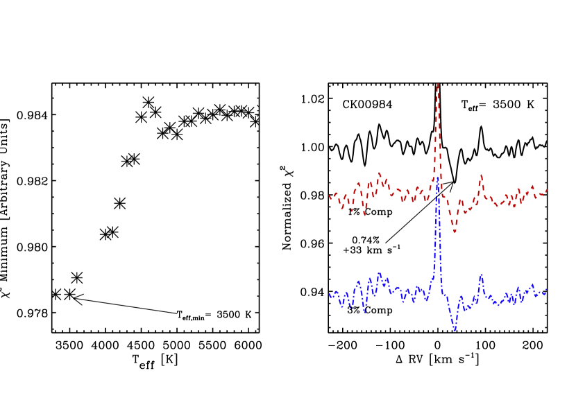
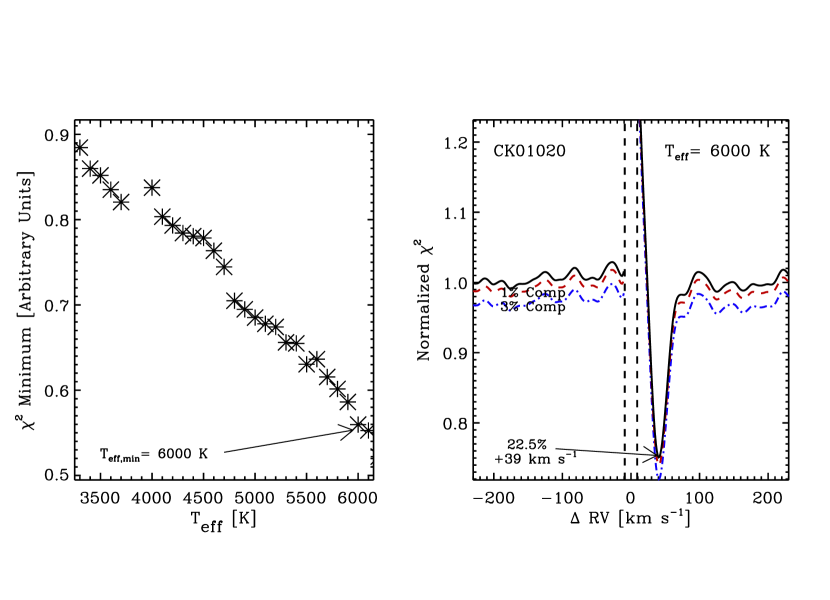
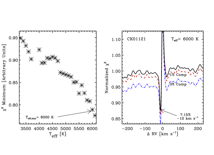
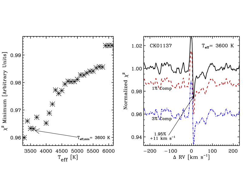
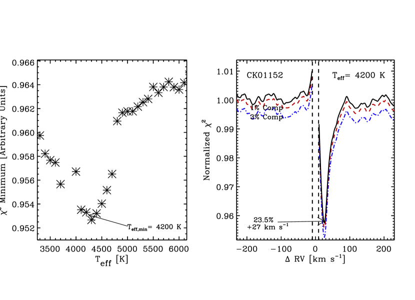
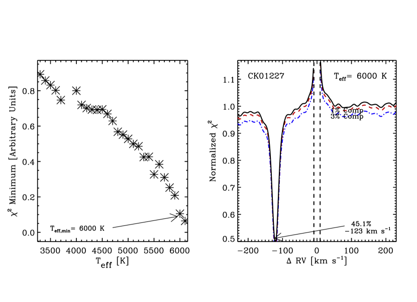
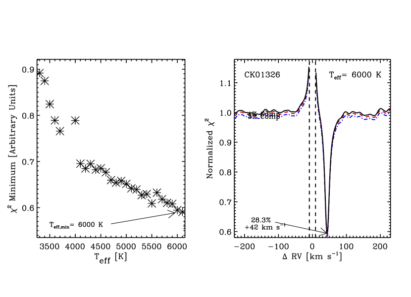
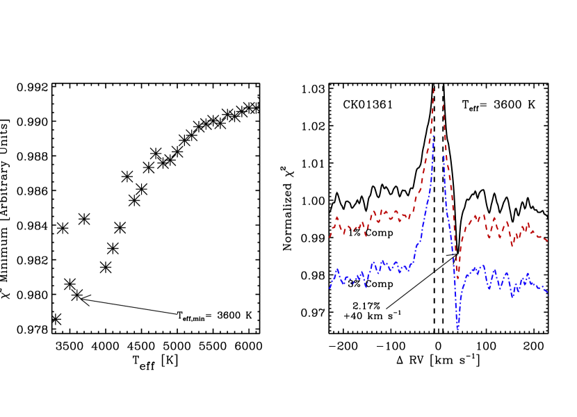
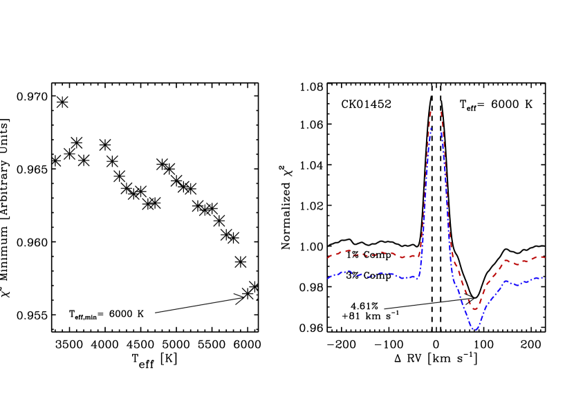
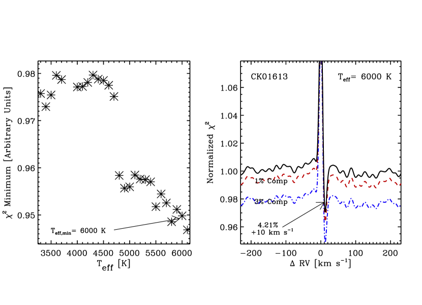
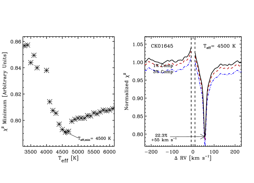
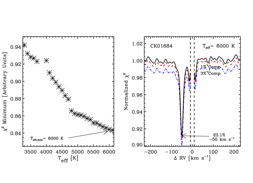
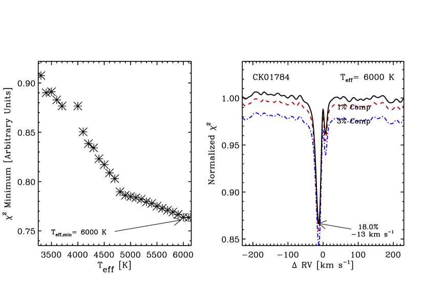
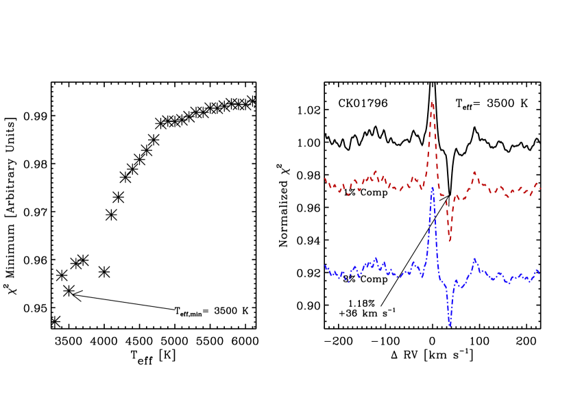
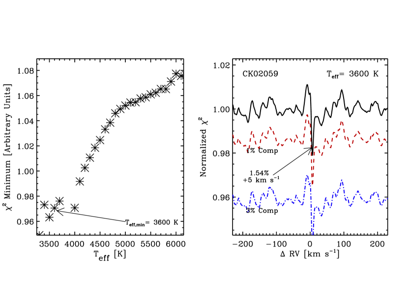
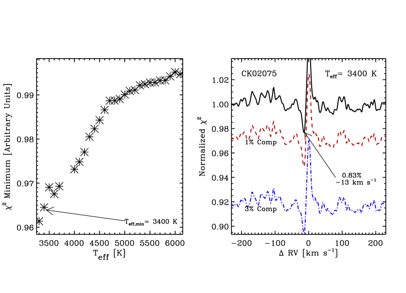
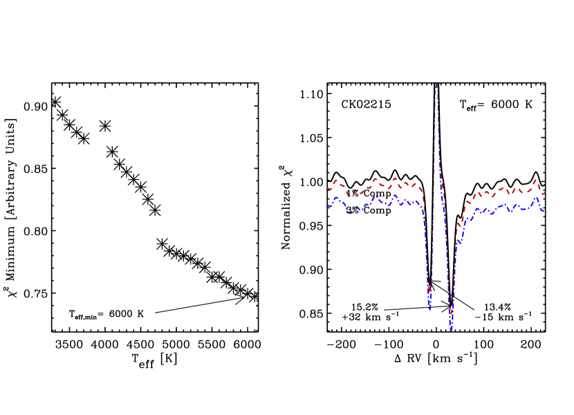
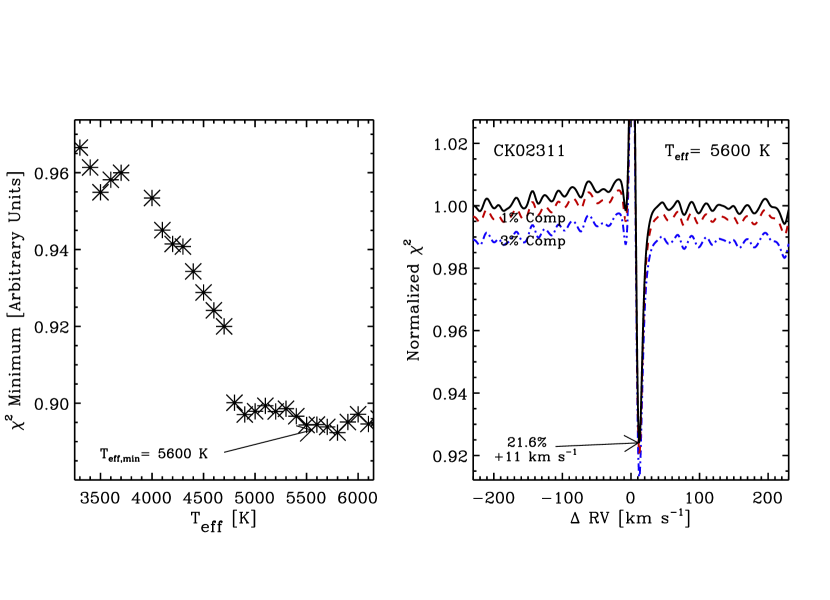
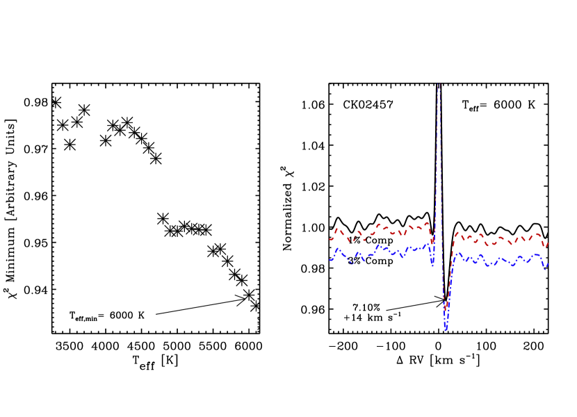
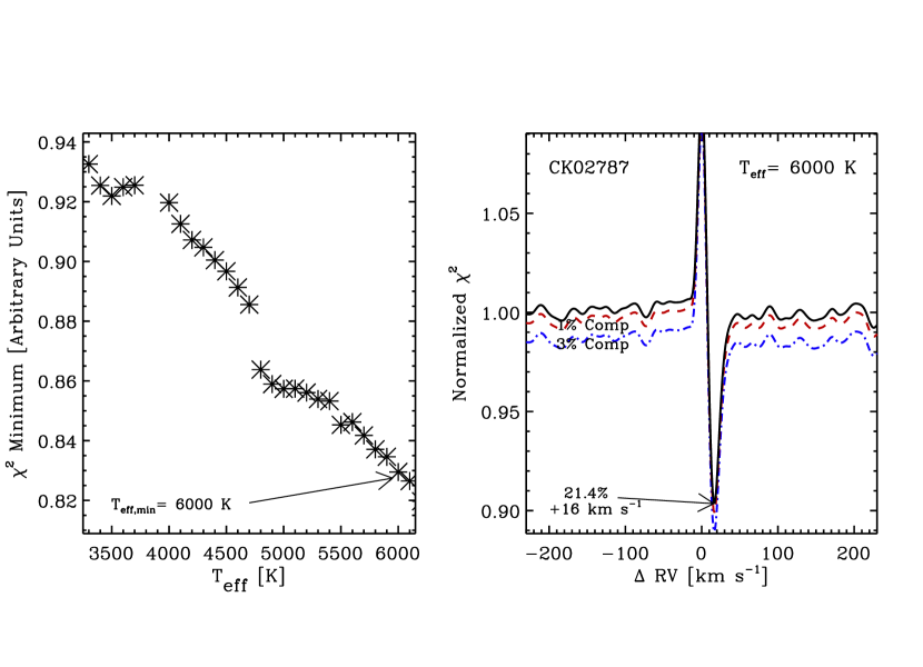
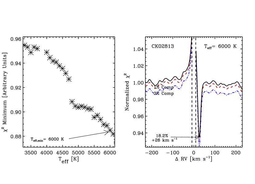
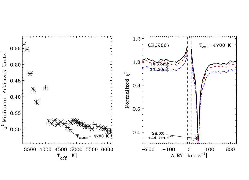
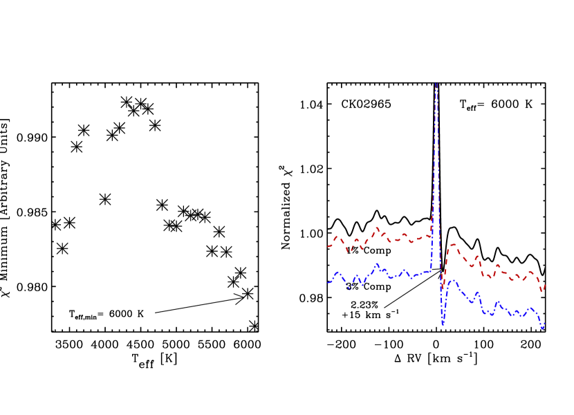
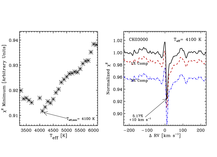
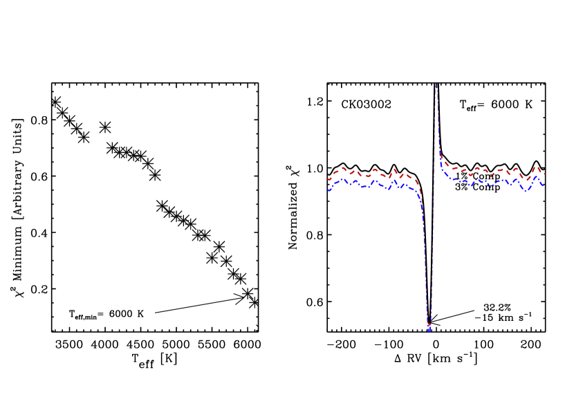
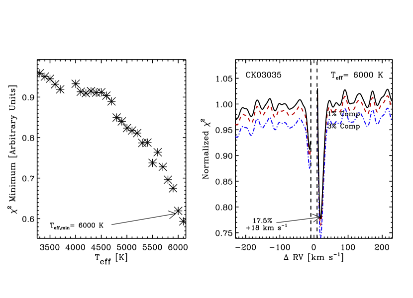
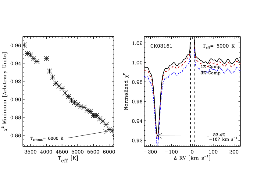
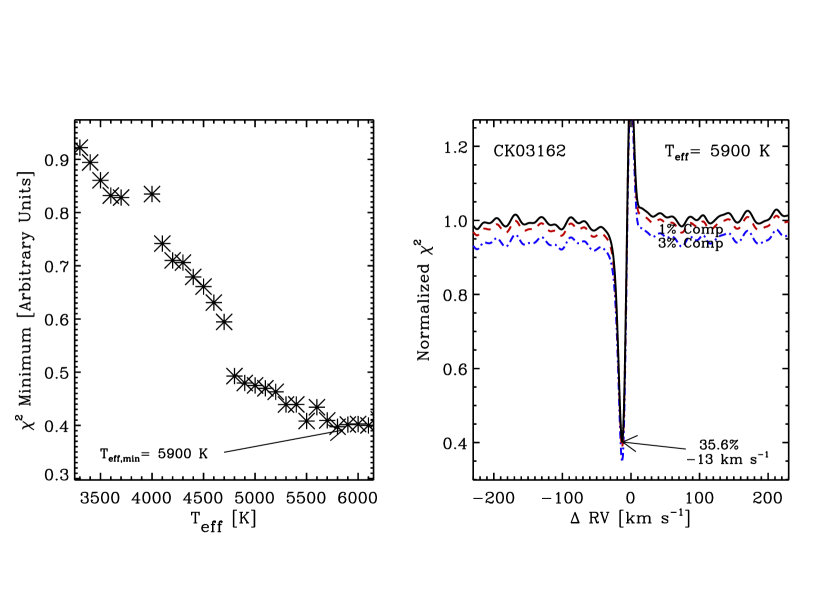
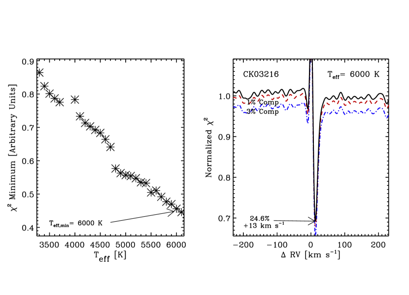
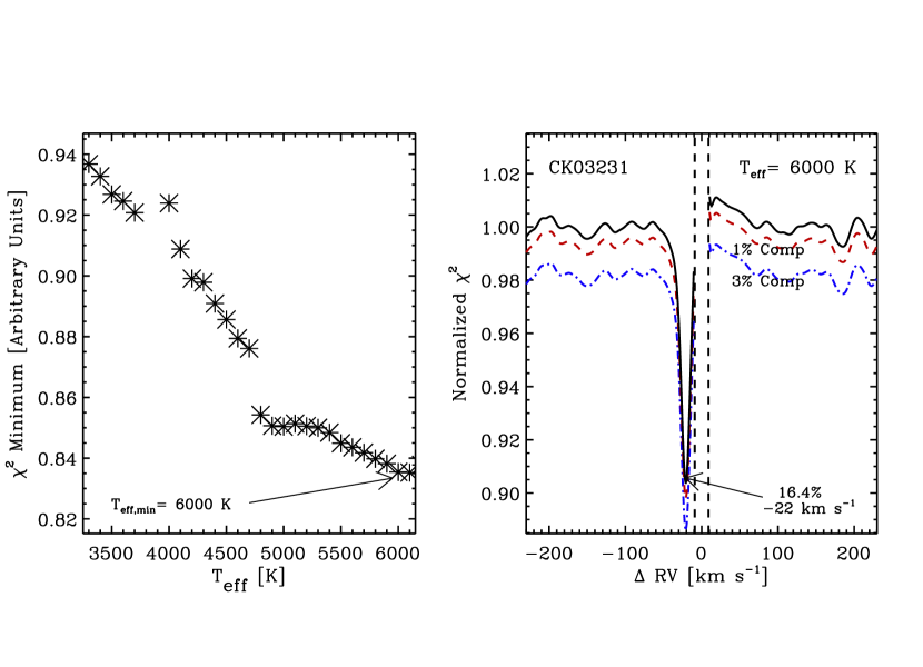
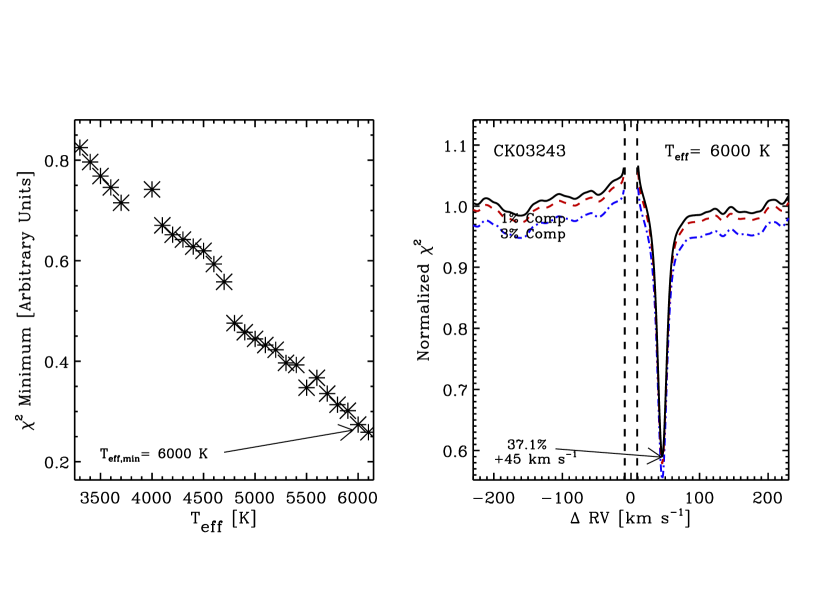
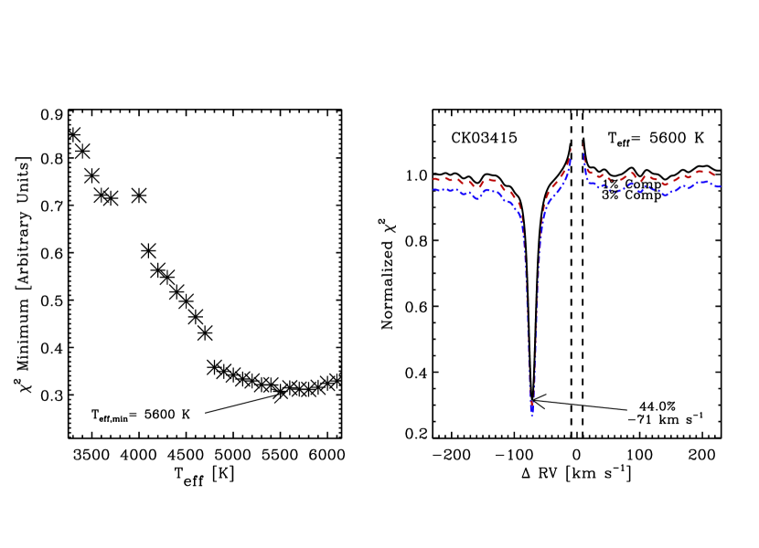
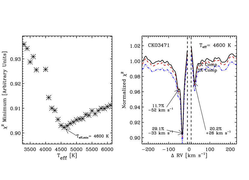
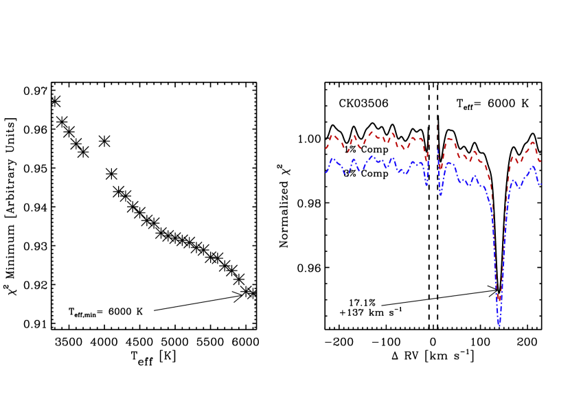
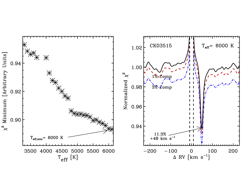
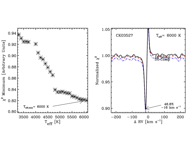
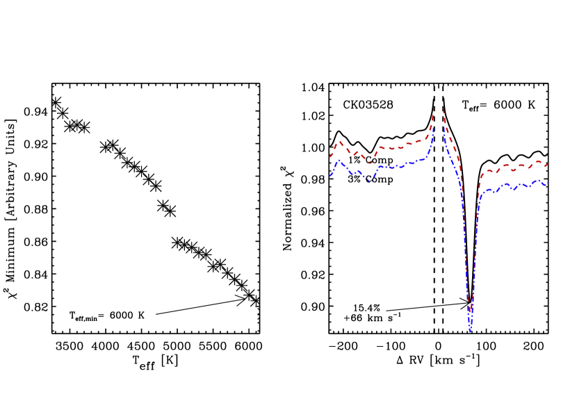
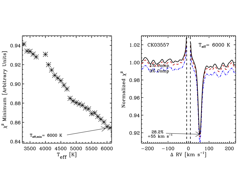
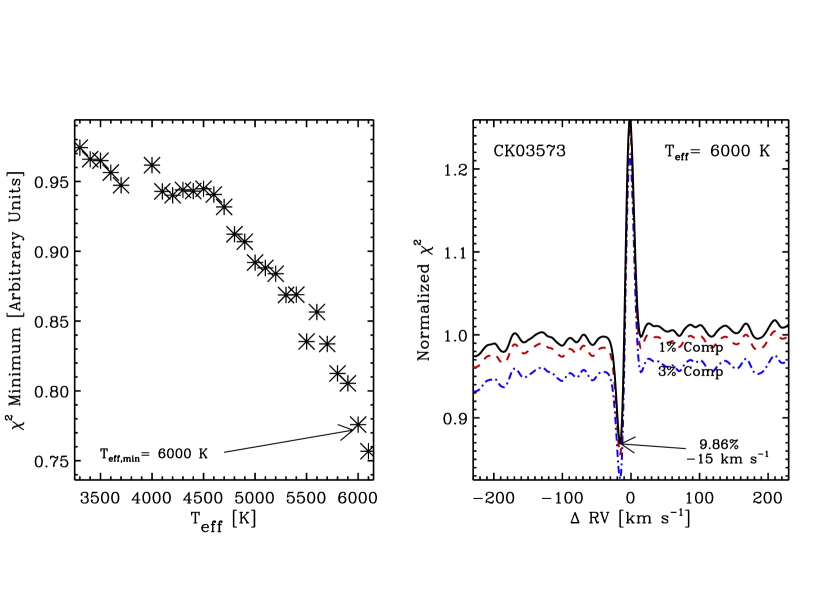
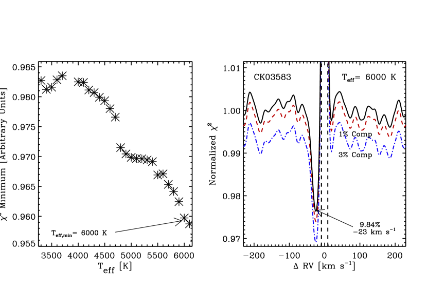
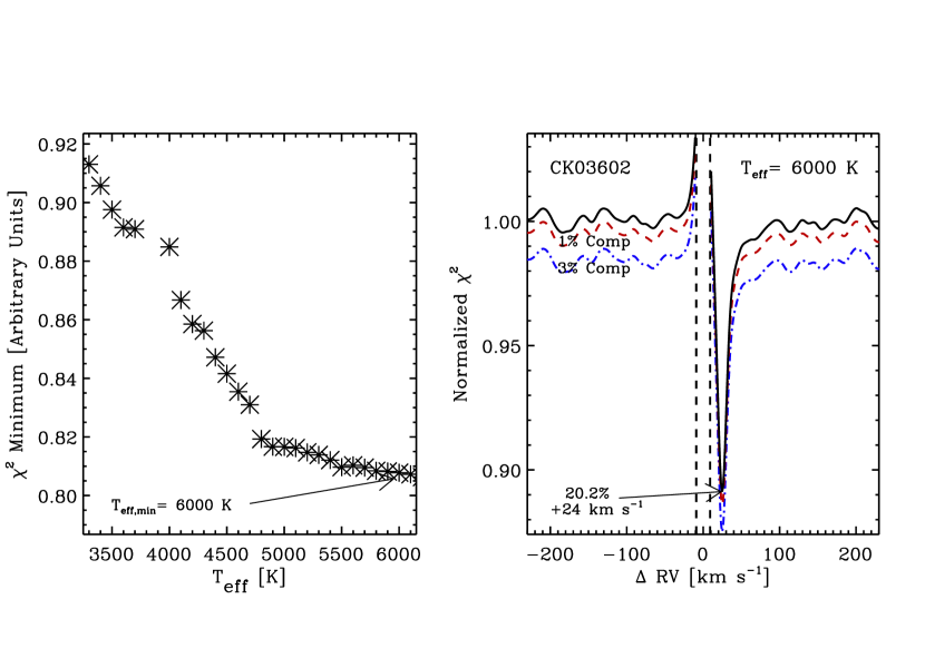
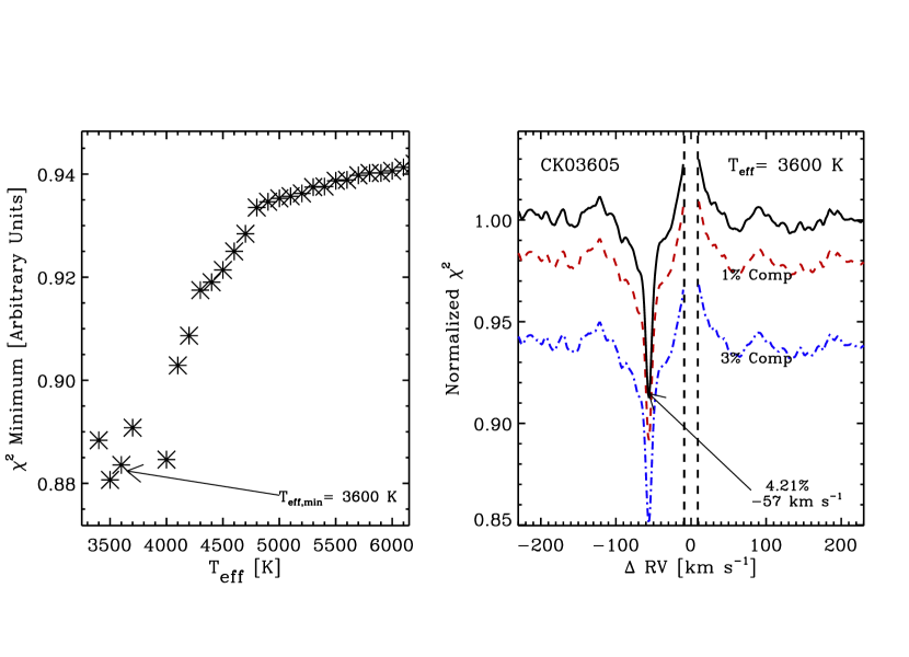
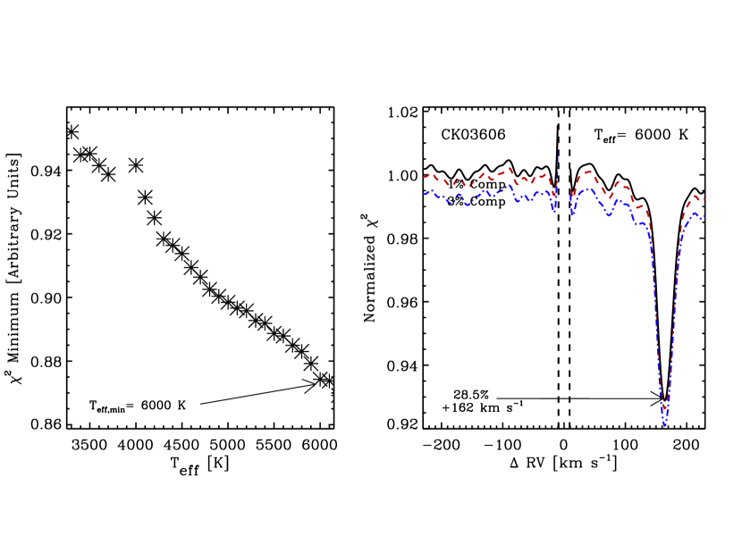
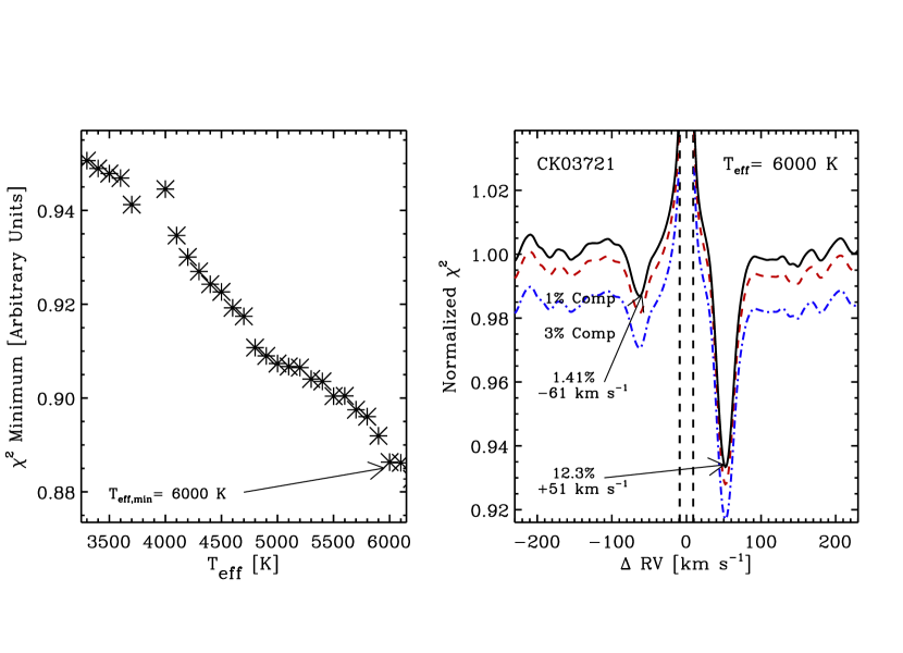
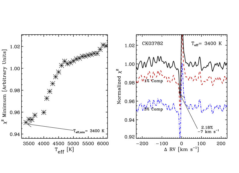
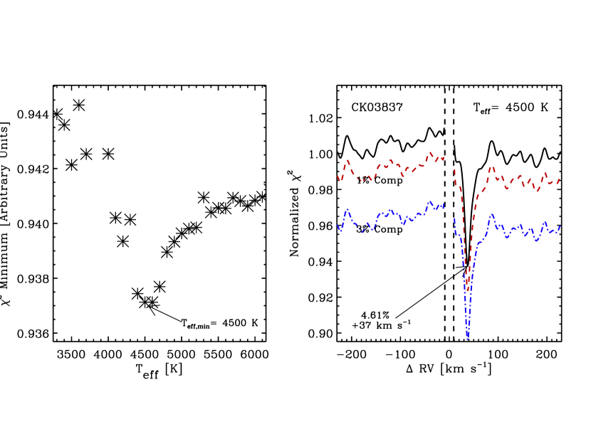
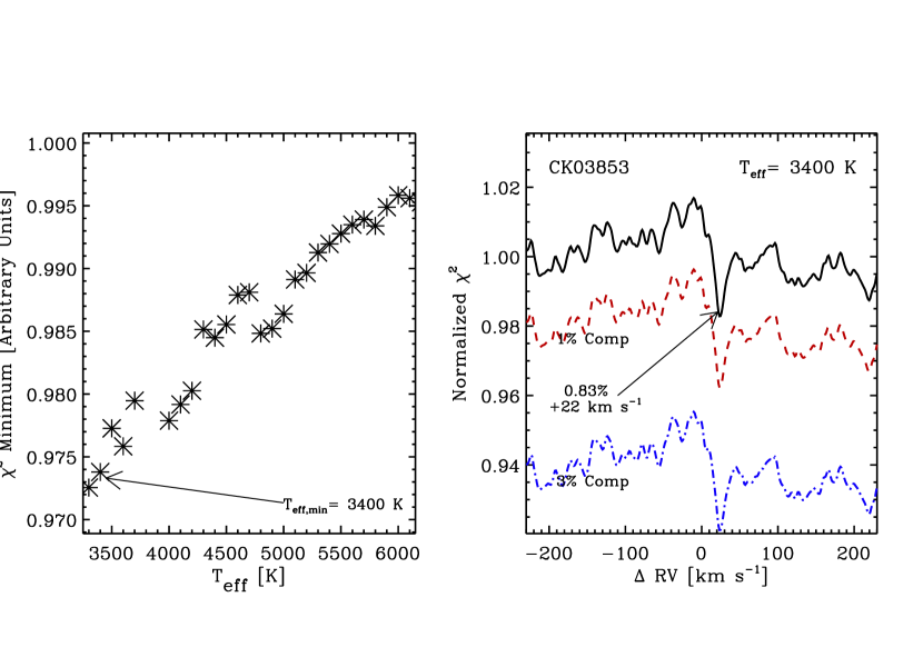
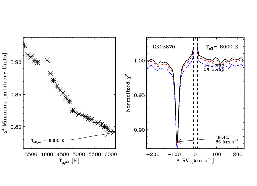
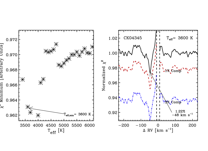
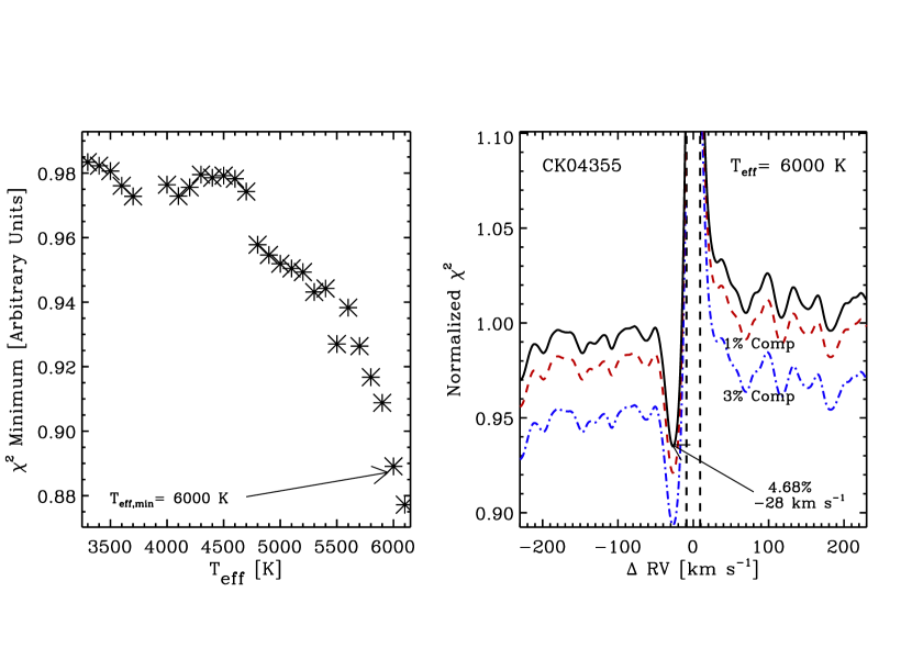
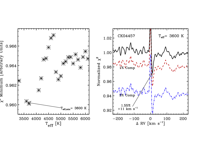
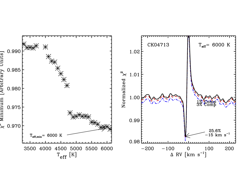
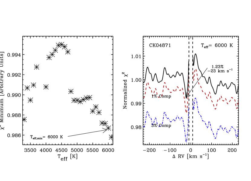
References
- Angus (2013) Angus, R. 2013, private communication
- Ballard et al. (2013) Ballard, S., Charbonneau,D., Fressin, F., et al. 2013, ApJ, 773, 98
- Batalha et al. (2013) Batalha, N. M., Rowe, J. F., Bryson, S. T., et al. 2013, ApJS, 204, 24
- Díaz et al. (2012) Díaz, R. F.,Santerne, A., Sahlmann, J., et al. 2012, A&A, 538, A113
- Fressin et al. (2013) Fressin, F., Torres, G., Charbonneau, D., et al. 2013, ApJ, 766, 81
- Hirano et al. (2012) Hirano, T., Sanchis-Ojeda, R., Takeda, Y., et al 2012, ApJ, 756, 66
- Law et al. (2014) Law, N. M., Morton, T., Baranec, C., et al. 2014, ApJ, 791, 35
- Marcy & Butler (1992) Marcy, G. W., & Butler, R. P. 1992, PASP, 104, 270
- Mazeh et al. (1993) Mazeh, T., Zucker, S., & Smith, H. 1993, in Bulletin of the American Astronomical Society, Vol. 25, American Astronomical Society Meeting Abstracts, 1425
- Morton & Johnson (2011) Morton, T. D., & Johnson, J. A. 2011, ApJ, 738, 170
- Raghavan et al. (2010) Raghavan, D., McAlister, H. A., Henry, T. J., et al. 2010, ApJS, 190, 1
- Rappaport et al. (2013) Rappaport, S., Deck, K., Levine, A., et al 2013, ApJ, 768, 33
- Rojas-Ayala et al. (2012) Rojas-Ayala, B., Covey, K. R., Muirhead, P. S., & Lloyd, J. P. 2012, ApJ, 748, 93
- Santerne et al. (2012) Santerne, A., Díaz, R. F., Moutou, C., et al. 2012, A&A, 545, A76
- Slawson et al. (2011) Slawson, R. W.,Prša, A., Welsh, W. F. et al. 2011, AJ, 142, 160
- Strassmeier et al. (2012) Strassmeier, K. G., Weber, M., Granzer, T., & Järvinen, S. 2012, Astronomische Nachrichten, 333, 663
- Valenti & Fischer (2005) Valenti, J. A., & Fischer, D. A. 2005, ApJS, 159, 141
- Wallace et al. (2011) Wallace, L., Hinkle, K. H., Livingston, W. C., & Davis, S. P. 2011, ApJS, 195, 6
- Wang et al. (2014) Wang, J., Xie, J.-W., Barclay, T., & Fischer, D. A. 2014, ApJ, 783, 4
- Welsh et al. (2011) Welsh, W. F., Orosz, J. A., Aerts, C., et al. 2011, ApJS, 197, 4
- Welsh et al. (2012) Welsh, W. F., Orosz, J. A., Carter, J. A., et al 2012, Nature, 481, 475