Two-photon total annihilation of molecular positronium

Abstract

The rate for complete two-photon annihilation of molecular positronium Ps₂ is reported. This decay channel involves a four-body collision among the fermions forming Ps₂, and two photons of 1.022 MeV, each, as the final state. The quantum electrodynamics result for the rate of this process is found to be $\Gamma_{Ps_{2}\rightarrow\gamma\gamma}$ = 9.0 $\times 10^{-12}$ s^-1. This decay channel completes the most comprehensive decay chart for Ps₂ up to date.

I Introduction

Positronium or Ps, is the bound state of an electron and its antiparticle, the positron, forming a metastable hydrogen-like atom Charlton and Humberston (2001). In the 1940’s, Wheeler speculated that two Ps atoms may form molecular positronium Ps₂, in analogy with two hydrogen atoms that can combine to form molecular hydrogen Wheeler (1946). In the same decade, calculations of the binding energy of Ps₂ were carried out, and it turned out to be 0.4 eV Hylleraas and Ore (1947), supporting Wheeler’s prediction. More recently, in 2007, Cassidy and Mills reported the first observation of molecular positronium Cassidy and Mills (2007).

Molecular positronium can decay to different final states or channels. The characterization of the decay channels is essential in order to estimate its lifetime. Moreover, the complete characterization of the Ps₂ decay channels and their partial widths could lead to the design of efficient detection schemes for this molecule. For a bound state, the total annihilation rate $\Gamma$ is determined as the sum of partial annihilation rates associated with each allowed decay channel $\Gamma_{i}$, i.e., $\Gamma=\sum_{i=1,N}\Gamma_{i}$, where $N$ represents the total number of decay channels. Each of the $\Gamma_{i}$ has to be computed by including all the topologically distinct Feynman diagrams associated with such channels, and in some cases, it can be important to include radiative corrections. Frolov has reported the most complete chart of decay channels as well as partial annihilation rates up to date Frolov (2009), including all the main decay channels, going from zero photon decay up to the 5-photon decay channel. However, a higher order decay channel of Ps₂ involving two-photons as the final state has not been considered in any estimation of the Ps₂ lifetime, and apparently never previously contemplated as a possible decay channel.

The present study reports the calculation of the two-photon complete annihilation rate of Ps₂, in which two electrons and two positrons annihilate simultaneously, producing two photons of 1.022 MeV energy each. The calculations have been carried out by using standard techniques of quantum field theory, such as the Feynman rules and trace technology Peskin and Schroeder (1995). This decay channel completes the decay chart of Ps₂, previously reported in part by Frolov Frolov (2009), besides the six-photon and seven-photon decay channels. While this decay is rare, it is worth mentioning that it provides a unique experimental signature of the presence of molecular positronium.

II Two-photon annihilation of Ps₂

The annihilation of Ps₂ into two photons (denoted here as Ps${}_{2}\rightarrow\gamma\gamma$) is governed by eight topological distinct Feynman diagrams. Four of them are shown in Fig.1. The rest of the diagrams emerge as cross terms of the ones shown in Fig. 1, i.e., in which the momenta of the outgoing photons are interchanged. Fig. 1 shows that the decay channel at hand is a four-body event, where the energy-momentum vectors of the incoming fermions are labelled as $p_{1}$, $p_{2}$, $p_{3}$, and $p_{4}$, whereas the energy-momenta of the outgoing photons are labelled as $k_{1}$ and $k_{2}$. Here, the energy-momentum vectors are represented as $(E,\vec{p})$, and natural units ($\hbar=c$ = 1, and $\alpha$ = 1/137, being fine structure constant) are assumed.

The momenta of the electrons and positrons in Ps₂ are very low in comparison with their rest mass energy. Hence the binding energy of the Ps₂ molecule is negligible in comparison with the rest mass energy of whatever of their constituents. Therefore, the first non-vanishing term in the amplitude expansion can be obtained by substitution of the initial energy-momentum vectors by $(m_{e},0,0,0)$, instead of the initial energy-momentum vectors. Here $m_{e}$ is the electron mass. Thus, in this approximation, the transition probability does not depend on the initial momenta $\vec{p}_{i}$. Within this approximation it is possible to establish a relationship between the annihilation rate and the probability to find the four fermions in the Ps₂ molecule to all be located at the same point in space. This information can be determined by generalizing the method employed for the calculation of the electron-positron annihilation rate of Ps Peskin and Schroeder (1995), but going beyond the two-body perspective of that reference. This generalization leads to:

$$\Gamma_{Ps_{2}\rightarrow\gamma\gamma}=\frac{|\Psi_{Ps_{2}}\left(0,0,0,0\right)|^{2}}{4}\int\frac{d^{3}\vec{k}_{1}}{\left(2\pi\right)^{3}2|\vec{k}_{1}|}\frac{d^{3}\vec{k}_{2}}{\left(2\pi\right)^{3}2|\vec{k}_{2}|}$$

$$\left(2\pi\right)^{4}\frac{\delta^{(4)}\left(p_{1}+p_{2}+p_{3}+p_{4}-k_{1}-k_{2}\right)}{\prod_{i=1,4}(2E_{i})}|\mathcal{M}|^{2}.$$

diagram1 (60,30) i2o4 $e^{-},p_{1}$i1$e^{+},p_{2}$i2 $e^{-},p_{3}$o1$e^{+},p_{4}$o2 photon,label=$\gamma$v5,v2 photon,label=$k_{1}$o3,v3 photon,label= $\ \ \ \ k_{2}$o4,v4 fermioni1,v5,i2 fermionv2,v3,o2 fermiono1,v4,v2 (0.75w,0.75h)v4 (0.6w,h)o1 (0.75w,0.25h)v3 (0.6w,0.0h)o2 (0.95w,0.25h)o3 (0.95w,0.75h)o4

diagram2 (60,30) i2o4 $e^{-},p_{1}$i1$e^{+},p_{2}$i2 $e^{-},p_{3}$o1$e^{+},p_{4}$o2 photon,label=$\gamma$v5,v2 photon,label=$k_{1}$o3,v3 photon,label= $\ \ \ \ k_{2}$o4,v4 fermioni1,v5,i2 fermiono1,v4,v3,v2 fermionv2,o2 (0.6w,0.5h)v2 (0.7w,0.8h)v4 (0.6w,h)o1 (0.7w,0.6h)v3 (0.85w,0.25h)o2 (0.9w,0.4h)o3 (0.95w,0.8h)o4

diagram3 (60,30) i2o4 $e^{-},p_{1}$i1$e^{+},p_{2}$i2 $e^{-},p_{3}$o1$e^{+},p_{4}$o2 photon,label=$\gamma$v5,v2 photon,label=$k_{1}$o3,v3 photon,label= $\ \ \ \ k_{2}$o4,v4 fermioni1,v5,i2 fermiono2,v4,v3,v2 fermionv2,o1 (0.6w,0.5h)v2 (0.6w,0.2h)v4 (0.8w,0.9h)o1 (0.7w,0.38h)v3 (0.5w,0h)o2 (0.9w,0.4h)o3 (0.85w,0.05h)o4

venga (60,30) i4o2 $e^{-},p_{1}$i1$e^{+},p_{2}$i2 $e^{-},p_{3}$i3$e^{+},p_{4}$i4 photon,label=$\gamma$v1,v3 photon,label=$k_{1}$o1,v2 photon,label= $\ \ \ \ k_{2}$o2,v4 fermioni1,v2,v1,i2 fermioni3,v4,v3,i4 (0.4w,0.15h)v2 (0.8w,0.15h)o1 (0w,0.7h)i4 (0.1w,1h)i3 (0.4w,0.85h)v4 (0.8w,0.85h)o2

Figure 1: Some of the Feynman diagrams associated to the two-photon decay channel of Ps₂, Ps${}_{2}\rightarrow\gamma\gamma$. There are four more Feynman diagrams that contribute to this decay channel, but they can be obtained as cross terms of the diagrams shown here, i.e., with interchanged momenta of the outgoing photons ($k_{1}\leftrightarrow k_{2}$).

The quantity $|\Psi_{Ps_{2}}\left(0,0,0,0\right)|^{2}$ represents the probability of finding the four fermions at the same point in position space. Some details about its calculation are given below. Eq. (II) can be viewed as an extension of the previous generalization of Kryuchkov Kryuchkov (1994) where a three body initial state was taken into account for the single photon decay of Ps^-. $\mathcal{M}$ represents the transition matrix associated with the decay channel, and therefore $|\mathcal{M}|^{2}$ represents the probability for such a transition. It is obtained by averaging the squared modulus of the total amplitude $\mathcal{A}$ over the spin states of the incoming particles [e^-($p_{1}$,$s_{1}$),e⁺($p_{2}$,$s_{2}$) ,e^-($p_{3}$,$s_{3}$),e⁺($p_{4}$,$s_{4}$), here $s_{i}$ represents the spin of each particle] and by summing over the polarizations of the outgoing particles [$\epsilon(k_{1})$, $\epsilon({k_{2}})$, here $\epsilon(k_{i})$ denotes the polarization of each photon], i.e.,

$$|\mathcal{M}|^{2}=\sum_{\epsilon(k_{1})}\sum_{\epsilon(k_{2})}\frac{1}{2^{4}}\sum_{s_{1}}\sum_{s_{2}}\sum_{s_{3}}\sum_{s_{4}}|\mathcal{A}|^{2}.$$ (2)

The amplitude $\mathcal{A}$ associated with the decay channel Ps${}_{2}\rightarrow\gamma\gamma$ contains eight terms, each of them associated with every Feynman diagram that contributes to the process (see Fig.1). The amplitude is given by

$$\mathcal{A}=e^{4}\bigg{[}\bar{v}(p_{4},s_{4})\gamma^{\lambda}\epsilon_{\lambda}(k_{1})\frac{\not{p}_{4}-\not{k}_{2}+m_{e}}{(p_{4}-k_{2})^{2}-m_{e}^{2}}\gamma^{\nu}$$

$$\times\frac{\not{p}_{3}-\not{k}_{1}+m_{e}}{(p_{3}-k_{1})^{2}-m_{e}^{2}}\gamma^{\sigma}\epsilon_{\sigma}(k_{1})u(p_{3},s_{3})$$

$$\times\frac{g_{\mu\nu}}{(p_{1}+p_{2})^{2}}\bar{v}(p_{2},s_{2})\gamma^{\mu}u(p_{1},s_{1})$$

$$+\bar{v}(p_{4},s_{4})\gamma^{\nu}\frac{\not{p}_{3}-\not{k}_{1}-\not{k}_{2}+m_{e}}{(p_{3}-k_{1}-k_{2})^{2}-m_{e}^{2}}\gamma^{\lambda}$$

$$\times\epsilon_{\lambda}(k_{2})\frac{\not{p}_{3}-\not{k}_{1}+m_{e}}{(p_{3}-k_{1})^{2}-m_{e}^{2}}\gamma^{\sigma}\epsilon_{\sigma}(k_{1})u(p_{3},s_{3})$$

$$\times\frac{g_{\mu\nu}}{(p_{1}+p_{2})^{2}}\bar{v}(p_{2},s_{2})\gamma^{\mu}u(p_{1},s_{1})$$

$$+\bar{v}(p_{4},s_{4})\gamma^{\sigma}\epsilon_{\sigma}(k_{1})\frac{\not{p}_{4}-\not{k}_{1}+m_{e}}{(p_{4}-k_{1})^{2}-m_{e}^{2}}\gamma^{\lambda}$$

$$\times\epsilon_{\lambda}(k_{2})\frac{\not{p}_{4}-\not{k}_{1}-\not{k}_{2}+m_{e}}{(p_{4}-k_{1}-k_{2})^{2}-m_{e}^{2}}\gamma^{\nu}u(p_{3},s_{3})$$

$$\times\frac{g_{\mu\nu}}{(p_{1}+p_{2})^{2}}\bar{v}(p_{2},s_{2})\gamma^{\mu}u(p_{1},s_{1})$$

$$+\bar{v}(p_{4},s_{4})\gamma^{\lambda}\epsilon_{\lambda}(k_{2})\frac{\not{p}_{4}-\not{k}_{2}+m_{e}}{(p_{4}-k_{2})^{2}-m_{e}^{2}}\gamma^{\nu}$$

$$\times u(p_{3},s_{3})\frac{g_{\mu\nu}}{(p_{2}+p_{1}-k_{1})^{2}}\bar{v}(p_{2},s_{2})\gamma^{\mu}$$

$$\frac{\not{p}_{1}-\not{k}_{1}+m_{e}}{(p_{1}-k_{1})^{2}-m_{e}^{2}}\gamma^{\sigma}\epsilon_{\sigma}(k_{1})u(p_{1},s_{1})+(k_{1}\leftrightarrow k_{2})\bigg{]},$$

Here the Feynman gauge has been employed as well as the slashed notation, i.e., $\not{p}=\gamma^{\nu}p_{\nu}$. The $\gamma$ matrices are related with the Dirac matrices as defined in Ref. Peskin and Schroeder (1995). Once the amplitude of the process is known $\mathcal{A}$, the transition probability associated with the decay channel at hand can be found, by means of Eq. (2). The calculations needed are rather involved, so they have been undertaken using the software program Mathematica Mat (2010), yielding

$$\Gamma_{Ps_{2}\rightarrow\gamma\gamma}=|\Psi_{Ps_{2}}\left(0,0,0,0\right)|^{2}\frac{521}{512}\frac{\pi^{3}}{2}\frac{\alpha^{4}}{m_{e}^{8}}.$$ (4)

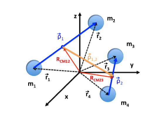
Figure 2: Jacobi coordinates for the four-body problem.

The Ps₂ ground state wave function has been obtained by using hyperspherical coordinates Hyp (1989) in conjunction with an explicitly correlated gaussian basis, following the method of Daily and Greene Daily and Greene (2014). In particular, the Ps₂ wave function is described in terms of the Jacobi coordinates depicted in Fig. 2, $\Psi_{Ps_{2}}(\rho_{1},\rho_{2},\rho_{1,2},\rho_{CM})$. After neglecting the center of (CM) motion (since the interaction potential does not depend on $\rho_{CM}$) and using adiabatic hyperspherical approximation, the wave function may be expressed as $\Psi_{Ps_{2}}(R,\Omega)$, where $R$ denotes the hyperradius and $\Omega$ labels the solid angle element associated to the eight hyperangles needed for the characterization of a four-body collision (neglecting the CM motion). Here the normalization condition for the wave function is

$$\frac{\int|\Psi_{Ps_{2}}(R,0)|^{2}R^{8}dR}{\int d\Omega}=1.$$ (5)

Finally, taking into account that $|\Psi_{Ps_{2}}(0,0,0,0)|^{2}=\frac{|\Psi_{Ps_{2}}(0,0)|^{2}}{\sqrt{\Omega}}$, one finds $|\Psi_{Ps_{2}}(0,0,0,0)|^{2}$=4.5$\times 10^{-6}$ a${}_{0}^{-9}$, with a₀ the Bohr radius. This value is in good agreement with the value reported previously by Frolov, 4.56 $\times 10^{-6}$ a${}_{0}^{-9}$ Frolov (2009).

After inserting the probability to find the four fermions at the same point $|\Psi_{Ps_{2}}(0,0,0,0)|^{2}$, the relation between atomic units and natural units, and after taking into account Eq. (4), we find $\Gamma_{Ps_{2}\rightarrow\gamma\gamma}$ = 9.0 $\times 10^{-12}$ s^-1. This decay rate is smaller than the alternative decay channels explored thus far, and which have been previously reported by Folov Frolov (2009). Table I shows a comparison between the rate for the two-photon decay and all the decay channels previously reported. Table I implies that the rate reported here, although smaller than the rest, is still comparable with the zero-photon decay channel. It is related with the number of vertices in each decay channel. The zero-photon decay involves three vertices ,whereas the two-photon decay channels require four vertices. This difference implies that $|\mathcal{M}|^{2}$ has an extra factor of $\alpha$ for the case of two-photon decay, in comparison with the zero-photon decay.

Table 1: Decay rates for Ps₂ molecule in (s^-1). The decay rates labelled as $\Gamma_{n\gamma}$, previous calculated by Frolov Frolov (2009), refers to the annihilation of electron-positron pairs in the Ps₂ molecule, being $n$ the number of photons emitted. Whereas $\Gamma_{Ps_{2}\rightarrow\gamma\gamma}$ stands for the four-body collision among the four fermions leading to the formation of two photons, see text for details.

Decay Channel		Decay rate (s-1)
$\Gamma_{0\gamma}$		2.32 $\times 10^{-9}$
$\Gamma_{1\gamma}$		1.94 $\times 10^{-1}$
$\Gamma_{2\gamma}$		4.44 $\times 10^{9}$
$\Gamma_{Ps_{2}\rightarrow\gamma\gamma}$		9.0 $\times 10^{-12}$
$\Gamma_{3\gamma}$		1.20 $\times 10^{7}$
$\Gamma_{4\gamma}$		6.56 $\times 10^{3}$
$\Gamma_{5\gamma}$		0.11 $\times 10^{2}$

III Conclusions

The two-photon annihilation rate of Ps₂ has been calculated using a non-relativistic reduction of quantum electrodynamic methods. This annihilation process refers to the simultaneous decay of two electrons and two positrons into two photons, providing a rare but unambiguously unique signature of the presence of the Ps₂ molecule. All the Feynman diagrams contributing to such process have been taken into account for the calculation of the transition probability. The wave function for ground state Ps₂ has been calculated by employing correlated Gaussian basis functions in combination with hyperspherical coordinates Daily and Greene (2014). The annihilation rate for this process turns out to be $\Gamma_{Ps_{2}\rightarrow\gamma\gamma}$ = 9.0 $\times 10^{-12}$ s^-1. While this value is smaller than that of other decay channels of Ps₂, it is nevertheless in the same range as the rate associated with the zero-photon decay Frolov (2009).

The observation of the event studied here will be very challenging due to its very long lifetime. However, from a fundamental point of view, the two-photon annihilation of Ps₂ constitutes a way to sample the Ps₂ wave function, from a four-body perspective, yielding crucial information about the nature of the bound state. Finally, we point out that in some astrophysical regions such as near the galactic center where a high density of positrons and electrons are available, this event may be observed, due to its unique emission signature of two photons with energies equal to 1.022 MeV. This region of the gamma ray spectra remains largely unexplored to date, although the International Gamma-Ray Astrophysics Laboratory (INTEGRAL) telescope has the capability for it. Indeed this telescope has found the signatures of two-photon annihilation in Ps Weidenspointner and et al (2006).

IV Acknowledgements

The authors would thank K. M. Daily for supplying the value of the Ps₂ wave function at the origin. S. T. L. thanks T. Clark for enjoyable discussions. This work was supported by the U.S. Department of Energy, Office of Science, Basic Energy Sciences, under Award number DE-SC0010545 (for J.P.-R. and C.H.G.).

References

- Charlton and Humberston (2001) M. Charlton and J. W. Humberston, Positron Physics (Cambridge Univ. Press., Cambridge, 2001).
- Wheeler (1946) J. A. Wheeler, Ann. NY Acad. Sci. 48, 219 (1946).
- Hylleraas and Ore (1947) E. A. Hylleraas and A. Ore, Phys. Rev. 71, 493 (1947).
- Cassidy and Mills (2007) D. B. Cassidy and A. P. J. Mills, Nature 449, 195 (2007).
- Frolov (2009) A. M. Frolov, Phys. Rev. A 80, 014502 (2009).
- Peskin and Schroeder (1995) M. E. Peskin and D. V. Schroeder, An Introduction to Quantum Field Theory (Westvie Press, 1995).
- Kryuchkov (1994) S. I. Kryuchkov, J. Phys. B 27, L61 (1994).
- Mat (2010) Mathematica, Wolfram Research, Inc., Champaign, Illinois, version 8.0 ed. (2010).
- Hyp (1989) Hyperspherical Harmonics: Applications in Quantum Theory (Kluwer, Norwell, MA, 1989).
- Daily and Greene (2014) K. M. Daily and C. H. Greene, Phys. Rev. A 89, 012503 (2014).
- Weidenspointner and et al (2006) G. Weidenspointner and et al, Astronomy and Astrophysics 450, 1013 (2006).