High performance computing and numerical modelling

Lecture Notes
 
43rd Saas-Fee Course
Star formation in galaxy evolution: connecting models to reality

1 Preamble

Numerical methods play an ever more important role in astrophysics. This can be easily demonstrated through a cursory comparison of a random sample of paper abstracts from today and 20 years ago, which shows that a growing fraction of studies in astronomy is based, at least in part, on numerical work. This is especially true in theoretical works, but of course, even in purely observational projects, data analysis without massive use of computational methods has become unthinkable. For example, cosmological inferences of large CMB experiments routinely use very large Monte-Carlo simulations as part of their Baysian parameter estimation.

The key utility of computer simulations comes from their ability to solve complex systems of equations that are either intractable with analytic techniques or only amenable to highly approximative treatments. Thanks to the rapid increase of the performance of computers, the technical limitations faced when attacking the equations numerically (in terms of calculational time, memory use, numerical resolution, etc.) become progressively smaller. But it is important to realize that they will always stay with us at some level. Computer simulations are therefore best viewed as a powerful complement to analytic reasoning, and as the method of choice to model systems that feature enormous physical complexity – such as star formation in evolving galaxies, the topic of this 43rd Saas Fee Advanced Course.

The organizers asked me to lecture about High performance computing and numerical modelling in this winter school, which took place March 11-16, 2013, in Villars-sur-Ollon, Switzerland. As my co-lecturers Ralf Klessen und Nick Gnedin should focus on the physical processes in the interstellar medium and on galactic scales, my task was defined as covering the basics of numerically treating gravity and hydrodynamics, and on making some remarks on the use of high performance computing techniques in general. In a nutshell, my lectures hence intend to cover the basic numerical methods necessary to simulate evolving galaxies. This is still a vast field, and I necessarily had to make a selection of a subset of the relevant material. I have tried to strike a compromise between what I considered most useful for the majority of students and what I could cover in the available time.

In particular, my lectures concentrate on techniques to compute gravitational dynamics of collisionless fluids composed of dark matter and stars in galaxies. I also spend a fair amount of time explaining basic concepts of various solvers for Eulerian gas dynamics. Due to lack of time, I am not discussing collisional N-body dynamics as applicable to star cluster, and I omit a detailed discussion of different schemes to implement adaptive mesh refinement.

The written notes presented here quite closely follow the lectures as held in Villars-sur-Ollon, apart from being expanded somewhat in detail where this seemed adequate. I note that the shear breadth of the material made it impossible to include detailed mathematical discussions and proofs of all the methods. The discussion is therefore often at an introductory level, but hopefully still useful as a general overview for students working on numerical models of galaxy evolution and star formation. Interested readers are referred to some of the references for a more detailed and mathematically sound exposition of the numerical techniques.

2 Collisionless N-body dynamics

According to the $\Lambda$CDM paradigm, the matter density of our Universe is dominated by dark matter, which is thought to be composed of a yet unidentified, non-baryonic elementary particle (e.g. Bertone et al., 2005). A full description of the dark mass in a galaxy would hence be based on following the trajectories of each dark matter particle – resulting in a gigantic N-body model. This is clearly impossible due to the large number of particles involved. Similarly, describing all the stars in a galaxy as point masses would require of order $10^{11}$ bodies. This may come within reach in a few years, but at present it is still essentially infeasible. In this section we discuss why we can nevertheless describe both of these galactic components as discrete N-body systems, but composed of far fewer particles than there are in reality.

2.1 The hierarchy of particle distribution functions

The state of an $N$-particle ensemble at time $t$ can be specified by the exact particle distribution function (Hockney & Eastwood, 1988), in the form

$$F(\vec{r},\vec{v},t)=\sum_{i=1}^{N}\delta(\vec{r}-\vec{r}_{i}(t))\cdot\delta(\vec{v}-\vec{v}_{i}(t)),$$ (1)

where $\vec{r}_{i}$ and $\vec{v}_{i}$ denote the position and velocity of particle $i$, respectively. This effectively gives the number density of particles at phase-space point $(\vec{r},\vec{v})$ at time $t$. Let now

$$p(\vec{r}_{1},\vec{r}_{2},\ldots,\vec{r}_{N},\vec{v}_{1},\vec{v}_{2},\ldots\vec{v}_{N})\,{\rm d}\vec{r}_{1}\,{\rm d}\vec{r}_{2}\cdots{\rm d}\vec{r}_{N}\,{\rm d}\vec{v}_{1}\,{\rm d}\vec{v}_{2}\cdots{\rm d}\vec{v}_{N},$$ (2)

be the probability that the system is in the given state at time $t$. Then a reduced statistical description is obtained by ensemble averaging:

$$f_{1}(\vec{r},\vec{v},t)=\left<F(\vec{r},\vec{v},t)\right>=\int F\cdot p\cdot{\rm d}\vec{r}_{1}\,{\rm d}\vec{r}_{2}\cdots{\rm d}\vec{r}_{N}\,{\rm d}\vec{v}_{1}\,{\rm d}\vec{v}_{2}\cdots{\rm d}\vec{v}_{N}.$$ (3)

We can integrate out one of the Dirac delta-functions in $F$ to obtain

$$f_{1}(\vec{r},\vec{v},t)=N\int p(\vec{r},\vec{r}_{2},\ldots,\vec{r}_{N},\vec{v},\vec{v}_{2},\ldots\vec{v}_{N})\,{\rm d}\vec{r}_{2}\cdots{\rm d}\vec{r}_{N}\,{\rm d}\vec{v}_{2}\cdots{\rm d}\vec{v}_{N}.$$ (4)

Note that as all particles are equivalent we can permute the arguments in $p$ where $\vec{r}$ and $\vec{v}$ appear. $f_{1}(\vec{r},\vec{v},t)\,{\rm d}\vec{r}\,{\rm d}\vec{v}$ now gives the mean number of particles in a phase-space volume ${\rm d}\vec{r}\,{\rm d}\vec{v}$ around $(\vec{r},\vec{v})$.

Similarly, the ensemble-averaged two-particle distribution (“the mean product of the numbers of particles at $(\vec{r},\vec{v})$ and $(\vec{r}^{\prime},\vec{v}^{\prime})$”) is given by

$$f_{2}(\vec{r},\vec{v},\vec{r}^{\prime},\vec{v}^{\prime},t)=\left<F(\vec{r},\vec{v},t)F(\vec{r}^{\prime},\vec{v}^{\prime},t)\right>$$ (5)

$$=N(N-1)\int p(\vec{r},\vec{r}^{\prime},\vec{r}_{3},\ldots,\vec{r}_{N},\vec{v},\vec{v}^{\prime},\vec{v}_{3},\ldots\vec{v}_{N})\,{\rm d}\vec{r}_{3}\cdots{\rm d}\vec{r}_{N}\,{\rm d}\vec{v}_{3}\cdots{\rm d}\vec{v}_{N}.$$

Likewise one may define $f_{3},f_{4},\ldots$ and so on. This yields the so-called BBGKY (Bogoliubov-Born-Green-Kirkwood-Yvon) chain (e.g. Kirkwood, 1946), see also Hockney & Eastwood (1988) for a detailed discussion.

Uncorrelated (collisionless) systems The simplest closure for the BBGKY hierarchy is to assume that particles are uncorrelated, i.e. that we have

$$f_{2}(\vec{r},\vec{v},\vec{r}^{\prime},\vec{v}^{\prime},t)=f_{1}(\vec{r},\vec{v},t)\,f_{1}(\vec{r}^{\prime},\vec{v}^{\prime},t).$$ (6)

Physically, this means that a particle at $(\vec{r},\vec{v})$ is completely unaffected by one at $(\vec{r}^{\prime},\vec{v}^{\prime})$. Systems in which this is approximately the case include stars in a galaxy, dark matter particles in the universe, or electrons in a plasma. We will later consider in more detail under which conditions a system is collisionless.

Let’s now go back to the probability density $p(\vec{w})$ which depends on the $N$-particle phase-space state $\vec{w}=(\vec{r}_{1},\vec{r}_{2},\ldots,\vec{r}_{N},\vec{v}_{1},\vec{v}_{2},\ldots\vec{v}_{N})$. The conservation of probability in phase-space means that it fulfills a continuity equation

$$\frac{\partial p}{\partial t}+\nabla_{\vec{w}}\cdot(p\,\vec{\dot{w}})=0.$$ (7)

We can cast this into

$$\frac{\partial p}{\partial t}+\sum_{i}\left(p\frac{\partial\vec{\dot{r}}_{i}}{\partial\vec{r}_{i}}+\frac{\partial p}{\partial\vec{r}_{i}}\vec{\dot{r}}_{i}+p\frac{\partial\vec{\dot{v}}_{i}}{\partial\vec{v}_{i}}+\frac{\partial p}{\partial\vec{v}_{i}}\vec{\dot{v}}_{i}\right)=0.$$ (8)

Because only conservative gravitational fields are involved, the system is described by classical mechanics as a so-called Hamiltonian system. Recalling the equations of motion $\vec{\dot{r}}=\frac{\partial H}{\partial\vec{p}}$ and $\vec{\dot{p}}=-\frac{\partial H}{\partial\vec{r}}$ of Hamiltonian dynamics (Goldstein, 1950), we can differentiate them to get $\frac{\partial\vec{\dot{r}}}{\partial\vec{r}}=\frac{\partial^{2}H}{\partial\vec{r}\partial\vec{p}}$, and $\frac{\partial\vec{\dot{p}}}{\partial\vec{p}}=-\frac{\partial^{2}H}{\partial\vec{r}\partial\vec{p}}$. Hence it follows $\frac{\partial\vec{\dot{r}}}{\partial\vec{r}}=-\frac{\partial\vec{\dot{v}}}{\partial\vec{v}}$. Using this we get

$$\frac{\partial p}{\partial t}+\sum_{i}\left(\vec{v}_{i}\frac{\partial p}{\partial\vec{r}_{i}}+\vec{a}_{i}\frac{\partial p}{\partial\vec{v}_{i}}\right)=0,$$ (9)

where $\vec{a}_{i}=\vec{\dot{v}}_{i}={\vec{F}_{i}}/{m_{i}}$ is the particle acceleration and $m_{i}$ is the particle mass. This is Liouville’s theorem.

Now, in the collisionless/uncorrelated limit, this directly carries over to the one-point distribution function $f=f_{1}$ if we integrate out all particle coordinates except for one as in equation (4), yielding the Vlasov equation, also known as collisionless Boltzmann equation:

$$\frac{\partial f}{\partial t}+\vec{v}\frac{\partial f}{\partial\vec{r}}+\vec{a}\frac{\partial f}{\partial\vec{v}}=0.$$ (10)

The close relation to Liouville’s equation means that also here the phase space-density stays constant along characteristics of the system (i.e. along orbits of individual particles).

What about the acceleration? In the limit of a collisionless system, the acceleration $\vec{a}$ in the above equation cannot be due to another single particle, as this would imply local correlations. However, collective effects, for example from the gravitational field produced by the whole system are still allowed.

For example, the source field of self-gravity (i.e. the mass density) can be described as

$$\rho(\vec{r},t)=m\int f(\vec{r},\vec{v},t)\,{\rm d}\vec{v}.$$ (11)

This then produces a gravitational field through Poisson’s equation,

$$\nabla^{2}\Phi(\vec{r},t)=4\pi G\rho(\vec{r},t),$$ (12)

which gives the accelerations as

$$\vec{a}=-\frac{\partial\Phi}{\partial\vec{r}}.$$ (13)

One can also combine these equations to yield the Poisson-Vlasov system, given by

$$\frac{\partial f}{\partial t}+\vec{v}\frac{\partial f}{\partial\vec{r}}-\frac{\partial\Phi}{\partial\vec{r}}\frac{\partial f}{\partial\vec{v}}=0,$$ (14)

$$\nabla^{2}\Phi=4\pi Gm\int f(\vec{r},\vec{v},t)\,{\rm d}\vec{v}.$$ (15)

This holds in an analogous way also for a plasma where the mass density is replaced by a charge density.

It is interesting to note that in this description the particles have basically completely vanished and have been replaced with a continuum fluid description. Later, for the purpose of solving the equations, we will have to reintroduce particles as a means of discretizing the equations – but these are then not the real physical particles any more, rather they are fiducial macro particles that sample the phase-space in a Monte-Carlo fashion.

2.2 The relaxation time – When is a system collisionless?

Consider a system of size $R$ containing $N$ particles. The time for one crossing of a particle through the system is of order

$$t_{\rm cross}=\frac{R}{v},$$ (16)

where $v$ is the typical particle velocity (Binney & Tremaine, 1987, 2008). For a self-gravitating system of that size we expect

$$v^{2}\simeq\frac{GNm}{R}=\frac{GM}{R},$$ (17)

where $M=N\,m$ is the total mass.

We now want to estimate the rate at which a particle experiences weak deflections by other particles, which is the process that violates perfect collisionless behavior and which induces relaxation. We calculate the deflection in the impulse approximation where the particle’s orbit is taken as a straight path, as sketched in Fig. 1.

7cm!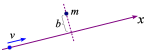

Figure 1: Sketch of a two-body encounter, in which a particle passes another particle (assumed to be at rest) with impact parameter $b$ and velocity $v$.

To get the deflection, we compute the transverse momentum acquired by the particle as it flies by the perturber (assumed to be stationary for simplicity):

$$\Delta p=m\Delta v=\int F_{\perp}{\rm d}t=\int\frac{Gm^{2}}{x^{2}+b^{2}}\frac{b}{\sqrt{x^{2}+b^{2}}}\frac{{\rm d}x}{v}=\frac{2Gm^{2}}{bv}.$$ (18)

How many encounters do we expect in one crossing? For impact parameters between $[b,b+{\rm d}b]$ we have

$${\rm d}n=N\frac{2\pi b\,{\rm d}b}{\pi R^{2}}$$ (19)

targets. The velocity perturbations from each encounter have random orientations, so they add up in quadrature. Per crossing we hence have for the quadratic velocity perturbation:

$$(\Delta v)^{2}=\int\left(\frac{2Gm}{bv}\right)^{2}{\rm d}n=8N\left(\frac{Gm}{Rv}\right)^{2}\ln\Lambda,$$ (20)

where

$$\ln\Lambda=\ln\frac{b_{\rm max}}{b_{\rm min}}$$ (21)

is the so-called Coulomb logarithm, and $b_{\rm max}$ and $b_{\rm min}$ are the adopted integration limits. We can now define the relaxation time as

$$t_{\rm relax}\equiv\frac{v^{2}}{(\Delta v)^{2}/t_{\rm cross}},$$ (22)

i.e. after this time the individual perturbations have reached $\sim 100\%$ of the typical squared velocity, and one can certainly not neglect the interactions any more. With our result for $(\Delta v)^{2}$, and using equation (17) this now becomes

$$t_{\rm relax}=\frac{N}{8\ln\Lambda}\,t_{\rm cross}.$$ (23)

But we still have to clarify what we can sensibly use for $b_{\rm min}$ and $b_{\rm max}$ in the Coulomb logarithm. For $b_{\rm max}$, we can set the size of the system, i.e. $b_{\rm max}\simeq R$. For $b_{\rm min}$, we can use as a lower limit the $b$ where very strong deflections ensue, which is given by

$$\frac{2Gm}{b_{\rm min}v}\simeq v,$$ (24)

i.e where the transverse velocity perturbation becomes as large as the velocity itself (see equation 18). This then yields $b_{\rm min}=2R/N$. We hence get for the Coulomb logarithm $\ln\Lambda\simeq\ln(N/2)$. But a factor of 2 in the logarithm might as well be neglected in this coarse estimate, so that we obtain $\ln\Lambda\sim N$. We hence arrive at the final result (Chandrasekhar, 1943):

$$t_{\rm relax}=\frac{N}{8\ln N}\,t_{\rm cross}.$$ (25)

A system can be viewed as collisionless if $t_{\rm relax}\gg t_{\rm age}$, where $t_{\rm age}$ is the time of interest. We note that $t_{\rm cross}$ depends only on the size and mass of the system, but not on the particle number $N$ or the individual masses of the N-body particles. We therefore clearly see that the primary requirement to obtain a collisionless system is to use a sufficiently large $N$.

Examples:

• globular star clusters have $N\sim 10^{5}$, $t_{\rm cross}\sim\frac{3\,{\rm pc}}{6\,{\rm km/sec}}\simeq 0.5\,{\rm Myr}$. This implies that such systems are strongly affected by collisions over the age of the Universe, $t_{\rm age}=\frac{1}{H_{0}}\sim 10\,{\rm Gyr}$, where $H_{0}$ is the Hubble constant.

• stars in a typical galaxy: Here we have $N\sim 10^{11}$ and $t_{\rm cross}\sim\frac{1}{100\,H_{0}}$. This means that these large stellar systems are collisionless over the age of the Universe to extremely good approximation.

• dark matter in a galaxy: Here we have $N\sim 10^{77}$ if the dark matter is composed of a $\sim 100\,{\rm GeV}$ weakly interacting massive particle (WIMP). In addition, the crossing time is longer than for the stars, $t_{\rm cross}\sim\frac{1}{10\,H_{0}}$, due to the larger size of the ‘halo’ relative to the embedded stellar system. Clearly, dark matter represents the crème de la crème of collisionless systems.

2.3 N-body models and gravitational softening

We now reintroduce particles in order to discretize the collisionless fluid described by the Poisson-Vlasov system. We use however far fewer particles than in real physical systems, and we correspondingly give them a higher mass. These are hence fiducial macro-particles. Their equations of motion in the case of gravity take on the form:

$$\vec{\ddot{x}}_{i}=-\nabla_{i}\Phi(\vec{r}_{i}),$$ (26)

$$\Phi(\vec{r})=-G\sum_{j=1}^{N}\frac{m_{j}}{[(\vec{r}-\vec{r}_{j})^{2}+\epsilon^{2}]^{1/2}}.$$ (27)

A few comments are in order here:

• Provided we can ensure $t_{\rm relax}\gg t_{\rm sim}$, where $t_{\rm sim}$ is the simulated time-space, the numerical model keeps behaving as a collisionless system over $t_{\rm sim}$ despite a smaller $N$ than in the real physical system. In this limit, the collective gravitational potential is sufficiently smooth.

• Note that the mass of a macro-particle used to discretize the collision system drops out from its equation of motion (because there is no self-force). Provided there are enough particles to describe the gravitational potential accurately, the orbits of the macro-particles will be just as valid as the orbits of the real physical particles.

• The N-body model gives only one (quite noisy) realization of the one-point function. It does not give the ensemble average directly (this would require multiple simulations).

• The equations of motion contain a softening length $\epsilon$. The purpose of the force softening is to avoid large angle scatterings and the numerical expense that would be needed to integrate the orbits with sufficient accuracy in singular potentials. Also, we would like to prevent the possibility of the formation of bound particle pairs – they would obviously be highly correlated and hence strongly violate collisionless behavior. We don’t get bound pairs if

  $$\left<v^{2}\right>\gg\frac{Gm}{\epsilon},$$ (28)

  which can be viewed as a necessary (but not in general sufficient) condition on reasonable softening settings (Power et al., 2003). The adoption of a softening length also implies the introduction of a smallest resolved length-scale. The specific softening choice one makes ultimately represents a compromise between spatial resolution, discreteness noise in the orbits and the gravitational potential, computational cost, and the relaxation effects that adversely influence results.

2.4 N-body equations in cosmology

In cosmological simulations, it is customary to use comoving coordinates $\vec{x}$ instead of physical coordinates $\vec{r}$. The two are related by

$$\vec{r}=a(t)\,\vec{x},$$ (29)

where $a=1/(1+z)$ is the cosmological scale factor. Its evolution is governed by the Hubble rate

$$\frac{\dot{a}}{a}=H(a),$$ (30)

which in turn is given by $H(a)=[\Omega_{0}a^{-3}+(1-\Omega_{0}-\Omega_{\Lambda})a^{-2}+\Omega_{\Lambda}]^{1/2}$ in standard Friedmann-Lemaitre models (e.g. Peacock, 1999; Mo et al., 2010).

In an (infinite) expanding space, modelled through period replication of a box of size $L$, one can then show (e.g. Springel et al., 2001) that the Newtonian equations of motion in comoving coordinates can be written as

$$\frac{{\rm d}}{{\rm d}t}(a^{2}\vec{\dot{x}})=-\frac{1}{a}\nabla_{i}\phi(\vec{x}_{i}),$$ (31)

$$\nabla^{2}\phi(\vec{x})=4\pi G\sum_{i}m_{i}\left[-\frac{1}{L^{3}}+\sum_{\vec{n}}\delta(\vec{x}-\vec{x}_{i}-\vec{n}L)\right],$$ (32)

where the sum over $i$ extends over $N$ particles in the box, and $\phi$ is the peculiar gravitational potential. It corresponds to the Newtonian potential of density deviations around a constant mean background density. Note that the sum over all particles for calculating the potential extends also over all of their period images, with $\vec{n}=(n_{1},n_{2},n_{3})$ being a vector of integer triples. The term $-1/L^{3}$ is simply needed to ensure that the mean density sourcing the Poisson equation vanishes, otherwise there would be no solution for an infinite space.

2.5 Calculating the dynamics of an N-body system

Once we have discretized a collisionless fluid in terms of an N-body system, two questions come up:

1. How do we integrate the equations of motion in time?

2. How do we compute the right hand side of the equations of motion, i.e. the gravitational forces?

For the first point, we can use an integration scheme for ordinary differential equations, preferably a symplectic one since we are dealing with a Hamiltonian system. We shall briefly discuss elementary aspects of these time integration methods in the following section.

The second point seems also straightforward at first, as the accelerations (forces) can be readily calculated through direct summation. In the isolated case this reads as

$$\vec{\ddot{r}}_{i}=-G\sum_{j=1}^{N}\frac{m_{j}}{[(\vec{r}_{i}-\vec{r}_{j})^{2}+\epsilon^{2}]^{3/2}}(\vec{r}_{i}-\vec{r}_{j}).$$ (33)

For a periodic space, the force kernel is slightly different but in principle the same summation applies (Hernquist et al., 1991). This calculation is exact, but for each of the $N$ equations we have to calculate a sum with $N$ partial forces, yielding a computational cost of order ${\cal O}(N^{2})$. This quickly becomes prohibitive for large $N$, and causes a conflict with our urgent need to have a large $N$!

Perhaps a simple example is in order to show how bad the $N^{2}$ scaling really is in practice. Suppose you can do $N=10^{6}$ in a month of computer time, which is close to the maximum that one may want to do in practice. A particle number of $N=10^{10}$ would then already take of order 10 million years.

We hence need faster, approximative force calculation schemes. We shall discuss a number of different possibilities for this in Section 4, namely:

• Particle-mesh (PM) algorithms

• Fourier-transform based solvers of Poisson’s equations

• Iterative solvers for Poisson’s equation (multigrid-methods)

• Hierarchical multipole methods (“tree-algorithms”)

• So-called TreePM methods

Various combinations of these approaches may also be used, and sometimes they are also applied together with direct summation on small scales. The latter may also be accelerated with special-purpose hardware (e.g. the GRAPE board; Makino et al., 2003), or with graphics processing units (GPUs) that are used as fast number-crushers.

3 Time integration techniques

We discuss in the following some basic methods for the integration of ordinary differential equations (ODEs). These are relations between an unknown scalar or vector-values function $\vec{y}(t)$ and its derivatives with respect to an independent variable, $t$ in this case (the following discussion associates the independent variable with ‘time’, but this could of course be also any other quantity). Such equations hence formally take the form

$$\frac{{\rm d}\vec{y}}{{\rm d}t}=\vec{f}(\vec{y},t),$$ (34)

and we seek the solution $\vec{y}(t)$, subject to boundary conditions.

Many simple dynamical problems can be written in this form, including ones that involve second or higher derivatives. This is done through a procedure called reduction to 1st order. One does this by adding the higher derivatives, or combinations of them, as further rows to the vector $\vec{y}$.

For example, consider a simple pendulum of length $l$ with the equation of motion

$$\ddot{q}=-\frac{g}{l}\sin(q),$$ (35)

where $q$ is the angle with respect to the vertical. Now define $p\equiv\dot{q}$, yielding a state vector

$$\vec{y}\equiv\left(\begin{array}[]{c}q\\ p\end{array}\right),$$ (36)

and a first order ODE of the form:

$$\frac{{\rm d}\vec{y}}{{\rm d}t}=\vec{f}(\vec{y})=\left(\begin{array}[]{c}p\\ -\frac{g}{l}\sin(q)\end{array}\right).$$ (37)

A numerical approximation to the solution of an ODE is a set of values $\{y_{0}$, $y_{1}$, $y_{2}$, $\ldots\}$ at discrete times $\{t_{0}$, $t_{1}$, $t_{2}$, $\ldots\}$, obtained for certain boundary conditions. The most common boundary condition for ODEs is the initial value problem (IVP), where the state of $\vec{y}$ is known at the beginning of the integration interval. It is however also possible to have mixed boundary conditions where $\vec{y}$ is partially known at both ends of the integration interval.

There are many different methods for obtaining a discrete solution of an ODE system (e.g. Press et al., 1992). We shall here discuss some of the most basic ones, restricting ourselves to the IVP problem, for simplicity, as this is the one naturally appearing in cosmological simulations.

3.1 Explicit and implicit Euler methods

Explicit Euler This solution method, sometimes also called “forward Euler”, uses the iteration

$$y_{n+1}=y_{n}+f(y_{n})\Delta t,$$ (38)

where $y$ can also be a vector. $\Delta t$ is the integration step.

• This approach is the simplest of all.

• The method is called explicit because $y_{n+1}$ is computed with a right-hand-side that only depends on quantities that are already known.

• The stability of the method can be a sensitive function of the step size, and will in general only be obtained for a sufficiently small step size.

• It is recommended to refrain from using this scheme in practice, since there are other methods that offer higher accuracy at the same or lower computational cost. The reason is that the Euler method is only first order accurate. To see this, note that the truncation error in a single step is of order ${\cal O}_{s}(\Delta t^{2})$, which follows simply from a Taylor expansion. To integrate over a time interval $T$, we need however $N_{s}=T/\Delta t$ steps, producing a total error that scales as $N_{s}{\cal O}_{s}(\Delta t^{2})={\cal O}_{T}(\Delta t)$.

• The method is also not time-symmetric, which makes it prone to accumulation of secular integration errors.

We remark in passing that for a method to reach a global error that scales as ${\cal O}_{T}(\Delta t^{n})$ (which is then called an “$n^{\rm th}$ order accurate” scheme), a local truncation error of one order higher is required, i.e. ${\cal O}_{s}(\Delta t^{n+1})$.

Implicit Euler In a so-called “backwards Euler” scheme, one uses

$$y_{n+1}=y_{n}+f(y_{n+1})\Delta t,$$ (39)

which seemingly represents only a tiny change compared to the explicit scheme.

• This approach has excellent stability properties, and for some problems, it is in fact essentially always stable even for extremely large timestep. Note however that the accuracy will usually nevertheless become very bad when using such large steps.

• This stability property makes implicit Euler sometimes useful for stiff equations, where the derivatives (suddenly) can become very large.

• The implicit equation for $y_{n+1}$ that needs to be solved here corresponds in many practical applications to a non-linear equation that can be complicated to solve for $y_{n+1}$. Often, the root of the equation has to be found numerically, for example through an iterative technique.

• The method is still first order accurate, and also lacks time-symmetry, just like the explizit Euler scheme.

Implicit midpoint rule If we use

$$y_{n+1}=y_{n}+f\left(\frac{y_{n}+y_{n+1}}{2}\right)\Delta t,$$ (40)

we obtain the implicit midpoint rule, which can be viewed as a symmetrized variant of explicit and implicit Euler. This is second order accurate, but still implicit, so difficult to use in practice. Interestingly, it is also time-symmetric, i.e. one can formally integrate backwards and recover exactly the same steps (modulo floating point round-off errors) as in a forward integration.

3.2 Runge-Kutta methods

The Runge-Kutta schemes form a whole class of versatile integration methods (e.g. Atkinson, 1978; Stoer & Bulirsch, 2002). Let’s derive one of the simplest Runge-Kutta schemes.

1. We start from the exact solution,

   $$y_{n+1}=y_{n}+\int_{t_{n}}^{t_{n+1}}f\left(y(t)\right){\rm d}t.$$ (41)

2. Next, we approximate the integral with the (implicit) trapezoidal rule:

   $$y_{n+1}=y_{n}+\frac{f(y_{n})+f(y_{n+1})}{2}\Delta t.$$ (42)

3. Runge (1895) proposed to predict the unknown $y_{n+1}$ on the right hand side by an Euler step, yielding a 2nd order accurate Runge-Kutta scheme, sometimes also called predictor-corrector scheme:

   $$k_{1} = f(y_{n},t_{n}),$$ (43)

   $$k_{2} = f(y_{n}+k_{1}\Delta t,t_{n+1}),$$ (44)

   $$y_{n+1} = \frac{k_{1}+k_{2}}{2}\Delta t.$$ (45)

   Here the step done with the derivate of equation (43) is called the ‘predictor’ and the one done with equation (44) is the corrector step.

Higher order Runge-Kutta schemes A variety of further Runge-Kutta schemes of different order can be defined. Perhaps the most commonly used is the classical $4^{\rm th}$-order Runge-Kutta scheme:

$$k_{1} = f(y_{n},t_{n}),$$ (46)

$$k_{2} = f\left(y_{n}+k_{1}\frac{\Delta t}{2},t_{n}+\frac{\Delta t}{2}\right),$$ (47)

$$k_{3} = f\left(y_{n}+k_{2}\frac{\Delta t}{2},t_{n}+\frac{\Delta t}{2}\right),$$ (48)

$$k_{4} = f\left(y_{n}+k_{3}\Delta t,t_{n}+\Delta t\right).$$ (49)

These four function evaluations per step are then combined in a weighted fashion to carry out the actual update step:

$$y_{n+1}=y_{n}+\left(\frac{k_{1}}{6}+\frac{k_{2}}{3}+\frac{k_{3}}{3}+\frac{k_{4}}{6}\right)\Delta t+{\cal O}(\Delta t^{5}).$$ (50)

We note that the use of higher order schemes also entails more function evaluations per step, i.e. the individual steps become more complicated and expensive. Because of this, higher order schemes are not always better; they usually are up to some point, but sometimes even a simple second-order accurate scheme can be the best choice for certain problems.

3.3 The leapfrog

Suppose we have a second order differential equation of the type

$$\ddot{x}=f(x).$$ (51)

This could of course be brought into standard form, $\dot{\vec{y}}=\vec{\tilde{f}}(\vec{y})$, by defining something like $\vec{y}=(x,\dot{x})$ and $\vec{\tilde{f}}=(\dot{x},f(x))$, followed by applying a Runge-Kutta scheme as introduced above.

However, there is also another approach in this case, which turns out to be particularly simple and interesting. Let’s define $v\equiv\dot{x}$. Then the so-called Leapfrog integration scheme is the mapping $(x_{n},v_{n})\to(x_{n+1},v_{n+1})$ defined as:

$$v_{n+\frac{1}{2}} = v_{n}+f(x_{n})\frac{\Delta t}{2},$$ (52)

$$x_{n+1} = x_{n}+v_{n+\frac{1}{2}}\,\Delta t,$$ (53)

$$v_{n+1} = v_{n+\frac{1}{2}}+f(x_{n+1})\frac{\Delta t}{2}.$$ (54)

• This scheme is 2nd-order accurate (proof through Taylor expansion).

• It requires only 1 evaluation of the right hand side per step (note that $f(x_{n+1})$ can be reused in the next step.

• The method is time-symmetric, i.e. one can integrate backwards in time and arrives at the initial state again, modulo numerical round-off errors.

• The scheme can be written in a number of alternative ways, for example by combining the two half-steps of two subsequent steps. One then gets:

  $$x_{n+1} = x_{n}+v_{n+\frac{1}{2}}\,\Delta t,$$ (55)

  $$v_{n+\frac{3}{2}} = v_{n+\frac{1}{2}}+f(x_{n+1})\,\Delta t.$$ (56)

  One here sees the time-centered nature of the formulation very clearly, and the interleaved advances of position and velocity give it the name leapfrog.

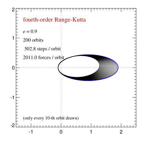
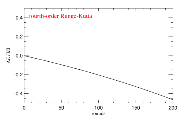
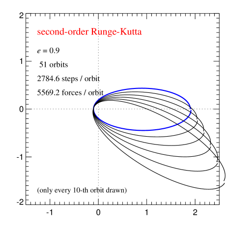
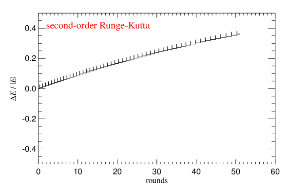
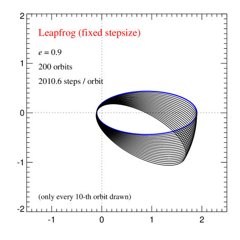
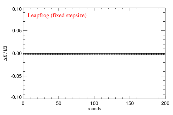
The performance of the leapfrog in certain problems is found to be surprisingly good, better than that of other schemes such as Runge-Kutta which have formally the same or even a better error order. This is illustrated in Figure 2 for the Kepler problem, i.e. the integration of the motion of a small point mass in the gravitational field of a large mass. We see that the long-term evolution is entirely different. Unlike the RK schemes, the leapfrog does not build up a large energy error. So why is the leapfrog behaving here so much better than other 2nd order or even 4th order schemes?

Figure 2: Kepler problem integrated with different integration schemes (Springel, 2005). The panels on top are for a 4th-order Runge Kutta scheme, the middle for a 2nd order Runge-Kutta, and the bottom for a 2nd-order leapfrog. The leapfrog does not show a secular drift of the total energy, and is hence much more suitable for long-term integration of this Hamiltonian system.

3.4 Symplectic integrators

The reason for these beneficial properties lies in the fact that the leapfrog is a so-called symplectic method. These are structure-preserving integration methods (e.g. Saha & Tremaine, 1992; Hairer et al., 2002) that observe important special properties of Hamiltonian systems: Such systems have first conserved integrals (such as the energy), they also exhibit phase-space conservation as described by the Liouville theorem, and more generally, they preserve Poincare’s integral invariants.

Symplectic transformations

• A linear map $F:\mathbb{R}^{2d}\to\mathbb{R}^{2d}$ is called symplectic if $\omega(F\xi,F\eta)=\omega(\xi,\eta)$ for all vectors $\xi,\eta\in\mathbb{R}^{2d}$, where $\omega$ gives the area of the parallelogram spanned by the the two vectors.

• A differentiable map $g:U\to\mathbb{R}^{2d}$ with $U\in\mathbb{R}$ is called symplectic if its Jacobian matrix is everywhere symplectic, i.e. $\omega(g^{\prime}\xi,g^{\prime}\eta)=\omega(\xi,\eta)$.

• Poincare’s theorem states that the time evolution generated by a Hamiltonian in phase-space is a symplectic transformation.

The above suggests that there is a close connection between exact solutions of Hamiltonians and symplectic transformations. Also, two consecutive symplectic transformations are again symplectic.

Separable Hamiltonians

Dynamical problems that are described by Hamiltonians of the form

$$H(p,q)=\frac{p^{2}}{2m}+U(q)$$ (57)

are quite common. These systems have separable Hamiltonians that can be written as

$$H(p,q)=H_{\rm kin}(p)+H_{\rm pot}(q).$$ (58)

Now we will allude to the general idea of operator splitting (Strang, 1968). Let’s try to solve the two parts of the Hamiltonian individually:

1. For the part $H=H_{\rm kin}=\frac{p^{2}}{2m}$, the equations of motion are

   $$\dot{q}=\frac{\partial H}{\partial p}=\frac{p}{m},$$ (59)

   $$\dot{p}=-\frac{\partial H}{\partial q}=0.$$ (60)

   These equations are straightforwardly solved and give

   $$q_{n+1} = q_{n}+\frac{p_{n}}{m}\Delta t,$$ (61)

   $$p_{n+1} = p_{n}.$$ (62)

   Note that this solution is exact for the given Hamiltonian, for arbitrarily long time intervals $\Delta t$. Given that it is a solution of a Hamiltonian, the solution constitutes a symplectic mapping.

2. The potential part, $H=H_{\rm pot}=U(q)$, leads to the equations

   $$\dot{q}=\frac{\partial H}{\partial p}=0,$$ (63)

   $$\dot{p}=-\frac{\partial H}{\partial q}=-\frac{\partial U}{\partial q}.$$ (64)

   This is solved by

   $$q_{n+1} = q_{n},$$ (65)

   $$p_{n+1} = p_{n}-\frac{\partial U}{\partial q}\Delta t.$$ (66)

   Again, this is an exact solution independent of the size of $\Delta t$, and therefore a symplectic transformation.

Let’s now introduce an operator $\varphi_{\Delta t}(H)$ that describes the mapping of phase-space under a Hamiltonian $H$ that is evolved over a time interval $\Delta t$. Then it is easy to see that the leapfrog is given by

$$\varphi_{\Delta t}(H)=\varphi_{\frac{\Delta t}{2}}(H_{\rm pot})\circ\varphi_{\Delta t}(H_{\rm kin})\circ\varphi_{\frac{\Delta t}{2}}(H_{\rm pot})$$ (67)

for a separable Hamiltonian $H=H_{\rm kin}+H_{\rm pot}$.

• Since each individual step of the leapfrog is symplectic, the concatenation of equation (67) is also symplectic.

• In fact, the leapfrog generates the exact solution of a modified Hamiltonian $H_{\rm leap}$, where $H_{\rm leap}=H+H_{\rm err}$. The difference lies in the ‘error Hamiltonian’ $H_{\rm err}$, which is given by

  $$H_{\rm err}\propto\frac{\Delta t^{2}}{12}\left\{\left\{H_{\rm kin},H_{\rm pot}\right\},H_{\rm kin}+\frac{1}{2}H_{\rm pot}\right\}+{\cal O}({\Delta t^{3}}),$$ (68)

  where the curly brackets are Poisson brackets (Goldstein, 1950). This can be demonstrated by expanding

  $${\rm e}^{(H+H_{\rm err})\Delta t}={\rm e}^{H_{\rm pot}\frac{\Delta t}{2}}\;{\rm e}^{H_{\rm kin}\Delta t}\;{\rm e}^{H_{\rm pot}\frac{\Delta t}{2}}$$ (69)

  with the help of the Baker-Campbell-Hausdorff formula (Campbell, 1897; Saha & Tremaine, 1992).

• The above property explains the superior long-term stability of the integration of conservative systems with the leapfrog. Because it respects phase-space conservation, secular trends are largely absent, and the long-term energy error stays bounded and reasonably small.

4 Gravitational force calculation

As mentioned earlier, calculating the gravitational forces exactly for a large number of bodies becomes computational prohibitive very quickly. Fortunately, in the case of collisionless systems, this is also not necessary, because comparatively large force errors can be tolerated. All they do is to shorten the relaxation time slightly by an insignificant amount (Hernquist et al., 1993). In this section, we discuss a number of the most commonly employed approximate force calculation schemes, beginning with the so-called particle mesh techniques (White et al., 1983; Klypin & Shandarin, 1983) that were originally pioneered in plasma physics (Hockney & Eastwood, 1988).

4.1 Particle mesh technique

An important approach to accelerate the force calculation for an N-body system lies in the use of an auxiliary mesh. Conceptually, this so-called particle-mesh (PM) technique involves four steps:

1. Construction of a density field $\rho$ on a suitable mesh.

2. Computation of the potential on the mesh by solving the Poisson equation.

3. Calculation of the force field from the potential.

4. Calculation of the forces at the original particle positions.

We shall now discuss these four steps in turn. An excellent coverage of the material in this section is given by Hockney & Eastwood (1988).

6cm!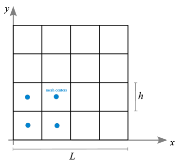

Figure 3: Sketch of the mesh geometry used in typical particle-mesh techniques with Cartesian grids.

Mass assignment

We want to put $N$ particles with mass $m_{i}$ and coordinates $\vec{r}_{i}$ ($i=1,2,\ldots,N$) onto a mesh with uniform spacing $h=L/N_{\rm g}$. For simplicity, we will assume a cubical calculational domain with extension $L$ and a number of $N_{\rm g}$ grid cells per dimension. Let $\{\vec{r}_{\vec{p}}\}$ denote the set of discrete cell-centers, with $\vec{p}=(p_{x},p_{y},p_{z})$ being a suitable integer index ($0\leq p_{x,y,z}<N_{g}$). Note that one may equally well identify the $\{\vec{r}_{\vec{p}}\}$ with the lower left corner of a mesh cell, if this is more practical.

We associate a shape function $S(\vec{x})$ with each particle, normalized according to

$$\int S(\vec{x})\,{\rm d}\vec{x}=1.$$ (70)

To each mesh-cell, we then assign the fraction $W_{\vec{p}}(\vec{x}_{i})$ of particle $i$’s mass that falls into the cell indexed by $\vec{p}$. This is given by the overlap of the mesh cell with the shape function, namely:

$$W_{\vec{p}}(\vec{x}_{i})=\int_{\vec{x}_{\vec{p}}-\frac{h}{2}}^{\vec{x}_{\vec{p}}+\frac{h}{2}}S(\vec{x}_{i}-\vec{x}_{\vec{p}})\,{\rm d}\vec{x}.$$ (71)

The integration extends here over the cubical cell $\vec{p}$. By introducing the top-hat function

$$\Pi(\vec{x})=\left\{\begin{array}[]{ll}1&\mbox{for $|\vec{x}|\leq\frac{1}{2}$},\\ 0&\mbox{otherwise},\end{array}\right.$$ (72)

we can extend the integration boundaries to all space and write instead:

$$W_{\vec{p}}(\vec{x}_{i})=\int\Pi\left(\frac{\vec{x}-\vec{x}_{\vec{p}}}{h}\right)\,S(\vec{x}_{i}-\vec{x}_{\vec{p}})\,{\rm d}\vec{x}.$$ (73)

Note that this also shows that the assignment function $W$ is a convolution of $\Pi$ with $S$. The full density in grid cell $\vec{p}$ is then given

$$\rho_{\vec{p}}=\frac{1}{h^{3}}\sum_{i=1}^{N}m_{i}W_{\vec{p}}(\vec{x}_{i}).$$ (74)

These general formula evidently depend on the specific choice one makes for the shape function $S(\vec{x})$. Below, we discuss a few of the most commonly employed low-order assignment schemes.

Nearest grid point (NGP) assignment

The simplest possible choice for $S$ is a Dirac $\delta$-function. One then gets:

$$W_{\vec{p}}(\vec{x}_{i})=\int\Pi\left(\frac{\vec{x}-\vec{x}_{\vec{p}}}{h}\right)\,\delta(\vec{x}_{i}-\vec{x}_{\vec{p}})\,{\rm d}\vec{x}=\Pi\left(\frac{\vec{x}_{i}-\vec{x}_{\vec{p}}}{h}\right).$$ (75)

In other words, this means that $W_{\vec{p}}$ is either 1 (if the coordinate of particle $i$ lies inside the cell), or otherwise it is zero. Consequently, the mass of particle $i$ is fully assigned to exactly one cell – the nearest grid point, as sketched in Figure 4.

7.5cm!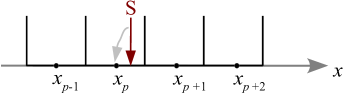

Figure 4: Sketch of the nearest grid point (NGP) assignment scheme. This simple binning scheme simply assigns the mass of a particle completely to the one mesh cell in which it falls.

Clouds-in-cell (CIC) assignment

Here one adopts as shape function

$$S(\vec{x})=\frac{1}{h^{3}}\Pi\left(\frac{\vec{x}}{h}\right),$$ (76)

which is the same cubical ‘cloud’ shape as that of individual mesh cells. The assignment function is

$$W_{\vec{p}}(\vec{x}_{i})=\int\Pi\left(\frac{\vec{x}-\vec{x}_{\vec{p}}}{h}\right)\,\frac{1}{h^{3}}\Pi\left(\frac{\vec{x}_{i}-\vec{x}_{\vec{p}}}{h}\right)\,{\rm d}\vec{x},$$ (77)

which only has a non-zero (and then constant) integrand if the cubes centered on $\vec{x}_{i}$ and $\vec{x}_{\vec{p}}$ overlap. How can this overlap be calculated? The 1D sketch of Fig. 5 can help to make this clear.

7.5cm!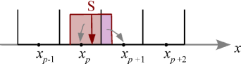

Figure 5: Sketch of the clouds-in-cell (CIC) assignment scheme. The fraction of mass assigned to a given cell is given by the fraction of the cubical cloud shape of the particle that overlaps with the cell.

Recall that for one of the dimensions we have $x_{p}=(p_{x}+1/2)h$, for $p\in\{0$, $1$, $2$, $\ldots$, $N-1\}$. For a given particle coordinate $x_{i}$ we may first calculate a ‘floating point index’ by inverting this relation, yielding $p_{f}=x_{i}/h-1/2$. The index of the left cell of the two cells with some overlap is then given by $p=\lfloor p_{f}\rfloor$, where the brackets denote the integer floor, i.e. the largest integer not larger than $p_{f}$. We may then further define $p^{\star}\equiv p_{f}-p$, which is a number between $0$ and $1$. From the sketch, we see that the length of the overlap of the particle’s cloud with the cell $p$ is $h-hp^{\star}$, hence the assignment function at cell $p$ takes on the value $W_{p}=1-m^{\star}$ for this location of the particle, whereas the assignment function for the neighboring cell $p+1$ will take on the value $W_{p+1}=m^{\star}$.

3.3cm!

Figure 6: Sketch of CIC assignment of a particle to a two-dimensional mesh.

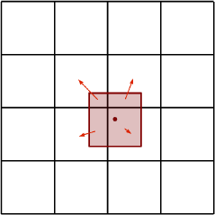
These considerations readily generalize to 2D and 3D. For example, in 2D (as sketched in Fig. 6), we first assign to the $y_{i}$-coordinate of point $i$ a ‘floating point index’ $q_{f}=y_{i}/h-1/2$. We can then use this to compute a cell index as the integer floor $q=\lfloor q_{f}\rfloor$, and a fractional contribution $q^{\star}=q_{f}-q$. Finally, we obtain the following weights for the assignment of a particle’s mass to the four cells its ‘cloud’ touches in 2D (as sketched):

$$W_{p,q} = (1-p^{\star})(1-q^{\star})$$ (78)

$$W_{p+1,q} = p^{\star}(1-q^{\star})$$ (79)

$$W_{p,q+1} = (1-p^{\star})q^{\star}$$ (80)

$$W_{p+1,q+1} = p^{\star}q^{\star}$$ (81)

In the corresponding 3D case, each particle contributes to the weight functions of 8 cells, or in other words, it is spread over 8 cells.

Triangular shaped clouds (TSC) assignment

One can construct a systematic sequence of ever higher-order shape functions by adding more convolutions with the top-hat kernel. For example, the next higher order (in 3D) is given by

$$W_{\vec{p}}(\vec{x}_{i}) = \int\Pi\left(\frac{\vec{x}-\vec{x}_{\vec{p}}}{h}\right)\,\frac{1}{h^{3}}\Pi\left(\frac{\vec{x}_{i}-\vec{x}-\vec{x}^{\prime}}{h}\right)\,\frac{1}{h^{3}}\Pi\left(\frac{\vec{x}^{\prime}}{h}\right)\,{\rm d}\vec{x}\,{\rm d}\vec{x}^{\prime}$$ (82)

$$= \frac{1}{h^{6}}\int\Pi\left(\frac{\vec{x}-\vec{x}_{\vec{p}}}{h}\right)\,\Pi\left(\frac{\vec{x}_{i}-\vec{x}}{h}\right)\,\Pi\left(\frac{\vec{x}^{\prime}-\vec{x}}{h}\right)\,{\rm d}\vec{x}\,{\rm d}\vec{x}^{\prime}.$$ (83)

This still has a simple geometric interpretation. If one pictures the kernel shape as a triangle with total base length $2h$, then the fraction assigned to a certain cell is given by the area of overlap of this triangle with the cell of interest (see Fig. 7). The triangle will now in general touch 3 cells per dimension, making an evaluation correspondingly more expensive. In 3D, 27 cells are touched for every particle.

7.5cm!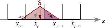

Figure 7: Sketch of triangular-shaped-clouds (TSC) assignment. Here a particle is spread to three cells in one dimension.

What’s the advantage of using TSC over CIC, if any? Or should one stick with the computationally cheap NGP? The assignment schemes differ in the smoothness and differentiability of the reconstructed density field. In particular, for NGP, the assigned density and hence the resulting force jump discontinuously when a particle crosses a cell boundary. The resulting force law will then at best be piece-wise constant.

In contrast, the CIC scheme produces a force that is piece-wise linear and continuous, but its first derivative jumps. Here the information where a particle is inside a certain cell is not completely lost, unlike in NGP.

Finally, TSC is yet smoother, and also the first derivative of the force is continuous. See Table 4.1 for a brief summary of these assignment schemes. Which of these schemes is the preferred choice is ultimately problem-dependent. In most cases, CIC and TSC are quite good options, providing sufficient accuracy with still reasonably small (and hence computationally efficient) assignment kernels. The latter get invariably more extended for higher-order assignment schemes, which not only is computationally ever more costly but also invokes additional communication overheads in parallelization schemes.

Table 1: Commonly used shape functions.

Name	Cloud shape $S(x)$	# of cells used	assignment function shape
NGP	$\delta(x)$	$1^{d}$	$\Pi$
CIC	$\frac{1}{h^{d}}\Pi\left(\frac{\vec{x}}{h}\right)$	$2^{d}$	$\Pi\star\Pi$
TSC	$\frac{1}{h^{d}}\Pi\left(\frac{\vec{x}}{h}\right)\star\frac{1}{h^{d}}\Pi\left(\frac{\vec{x}}{h}\right)$	$3^{d}$	$\Pi\star\Pi\star\Pi$

Solving for the gravitational potential

Once the density field is obtained, we would like to solve Poisson’s equation

$$\nabla^{2}\Phi=4\pi G\,\rho,$$ (84)

and obtain the gravitational potential discretized on the same mesh. There are primarily two methods that are in widespread use for this.

First, there are Fourier-transform based methods which exploit the fact that the potential can be viewed as a convolution of a Green’s function with the density field. In Fourier-space, one can then use the convolution theorem and cast the computationally expensive convolution into a cheap algebraic multiplication. Due to the importance of this approach, we will discuss it extensively in subsection 4.2.

Second, there are also iterative solvers for Poisson’s equation which yield a solution directly in real-space. Simple versions of such iteration schemes use Jacobi or Gauss-Seidel iteration, more complicated ones employ a sophisticated multi-grid approach to speed up convergence. We shall discuss these methods in subsection 4.3.

Calculation of the forces

Let’s assume for the moment that we already obtained the gravitational potential $\Phi$ on the mesh, with one of the methods mentioned above. We would then like to get the acceleration field from

$$\vec{a}=-\nabla\Phi.$$ (85)

One can achieve this by calculating a numerical derivative of the potential by finite differencing. For example, the simplest estimate of the force in the $x$-direction would be

$$a_{x}^{(i,j,k)}=-\frac{\Phi^{(i+1,j,k)}-\Phi^{(i-1,j,k)}}{2h},$$ (86)

where $\vec{p}=(i,j,k)$ is a cell index. The truncation error of this expression is ${\cal O}(h^{2})$, hence the estimate of the derivative is second-order accurate.

Alternatively, one can use larger stencils to obtain a more accurate finite difference approximation of the derivative, at greater computational cost. For example, the 4-point expression

$$a_{x}^{(i,j,k)}=-\frac{1}{2h}\left\{\frac{4}{3}\left[\Phi^{(i+1,j,k)}-\Phi^{(i-1,j,k)}\right]-\frac{1}{6}\left[\Phi^{(i+2,j,k)}-\Phi^{(i-2,j,k)}\right]\right\}$$ (87)

can be used, which has a truncation error of ${\cal O}(h^{4})$, as verified through simple Taylor expansions.

For the $y$- and $z$-dimensions, corresponding formulae, where $j$ or $k$ are varied and the other cell coordinates are held fixed, can be used. Whether a second- or fourth-order discretization formula should be used depends again on the question which compromise between accuracy and speed is best for a given problem. In many collisionless simulation set-ups, the residual truncation error of the second-order finite difference approximation of the force will be negligible compared to other errors inherent in the simulation methodology, hence the second-order formula would then be expected to be sufficient. But this cannot be generalized to all situations and simulation setups; if in doubt, it is best to explicitly test for this source of error.

Interpolating from the mesh to the particles

Once we have the force field on a mesh, we are not yet fully done. We actually desire the forces at the particle coordinates of the N-body system, not at the coordinates of the mesh cells of our auxiliary computational grid. We are hence left with the problem of interpolating the forces from the mesh to the particle coordinates.

Recall that we defined the density field in terms of mass assignment functions, of the form

$$\rho_{\vec{p}}=\frac{1}{h^{3}}\sum_{i}W_{\vec{p}}(\vec{x}_{i})=\frac{1}{h^{3}}\sum_{i}W(\vec{x}_{i}-\vec{x}_{\vec{p}}).$$ (88)

Here we introduced in the last expression an alternative notation for the weight assignment function.

Assume that we have computed the acceleration field on the grid, $\{\vec{a}_{\vec{p}}\}$. It turns out to be very important to use the same assignment kernel as used in the density construction also for the force interpolation, i.e. the force at coordinate $\vec{x}$ for a mass $m$ needs to be computed as

$$\vec{F}(\vec{x})=m\sum_{\vec{p}}\vec{a}_{\vec{p}}W(\vec{x}-\vec{x}_{\vec{p}}),$$ (89)

where $W$ denotes the assignment function used for computing the density field on the mesh. This requirement results from the desire to have a vanishing self-force, as well as pairwise antisymmetric forces between every particle pair. The self-force is the force that a particle would feel if just it alone would be present in the system. If numerically this force would evaluate to a non-zero value, the particle would accelerate all by itself, violating momentum conservation. Likewise, for two particles, we require that the forces they mutually exert on each other are equal in magnitude and opposite in direction, such that momentum conservation is manifest.

We now show that using the same kernels for the mass assignment and force interpolation protects against these numerical artefacts (Hockney & Eastwood, 1988). We start by noting that the acceleration field at a mesh point $\vec{p}$ depends linearly on the mass at another mesh point $\vec{p}^{\prime}$, which is a manifestation of the superposition principle (this can, for example, also be seen when Fourier techniques are used to solve the Poisson equation). We can hence express the field as

$$\vec{a}_{\vec{p}}=\sum_{\vec{p}^{\prime}}\vec{d}(\vec{p},\vec{p}^{\prime})\,h^{3}\rho_{\vec{p}^{\prime}},$$ (90)

with a Green’s function $\vec{d}(\vec{p},\vec{p}^{\prime})$. This vector-valued Green’s function for the force is antisymmetric, i.e. it changes sign when the two points in the arguments are swapped. Note that $h^{3}\rho_{\vec{p}^{\prime}}$ is simply the mass contained in mesh cell $\vec{p}^{\prime}$.

We can now calculate the self-force resulting from the density assignment and interpolation steps:

$$\vec{F}_{\rm self}(\vec{x}_{i}) = m_{i}\vec{a}_{i}(\vec{x}_{i})=m_{i}\sum_{\vec{p}}W(\vec{x}_{i}-\vec{x}_{\vec{p}})\vec{a}_{\vec{p}}$$ (91)

$$= m_{i}\sum_{\vec{p}}W(\vec{x}_{i}-\vec{x}_{\vec{p}})\sum_{\vec{p}^{\prime}}\vec{d}(\vec{p},\vec{p}^{\prime})h^{3}\rho_{\vec{p}^{\prime}}$$ (92)

$$= m_{i}\sum_{\vec{p}}W(\vec{x}_{i}-\vec{x}_{\vec{p}})\sum_{\vec{p}^{\prime}}\vec{d}(\vec{p},\vec{p}^{\prime})m_{i}W(\vec{x}_{i}-\vec{x}_{\vec{p}^{\prime}})$$ (93)

$$= m_{i}^{2}\sum_{\vec{p},\vec{p}^{\prime}}\vec{d}(\vec{p},\vec{p}^{\prime})W(\vec{x}_{i}-\vec{x}_{\vec{p}})W(\vec{x}_{i}-\vec{x}_{\vec{p}^{\prime}})$$ (94)

$$= 0.$$ (95)

Here we have started out with the interpolation from the mesh-based acceleration field, and then inserted the expansion of the latter as as convolution over the density field of the mesh. Finally, we put in the density contribution created by the particle $i$ at a mesh cell $\vec{p}^{\prime}$. We then see that the double sum vanishes because of the antisymmetry of ${\vec{d}}$ and the symmetry of the kernel product under exchange of $\vec{p}$ and $\vec{p}^{\prime}$. Note that this however only works because the kernels used for force interpolation and density assignment are indeed equal – it would have not worked out if they would be different, which brings us back to the point emphasized above.

Now let’s turn to the force antisymmetry. The force exerted on a particle 1 of mass $m_{1}$ at location $\vec{x}_{1}$ due to a particle 2 of mass $m_{2}$ at location $\vec{x}_{2}$ is given by

$$\vec{F}_{12} = m_{1}\vec{a}(\vec{x}_{1})=m_{1}\sum_{\vec{p}}W(\vec{x}_{1}-\vec{x}_{\vec{p}})\vec{a}_{\vec{p}}$$ (96)

$$= m_{1}\sum_{\vec{p}}W(\vec{x}_{1}-\vec{x}_{\vec{p}})\sum_{\vec{p}^{\prime}}\vec{d}(\vec{p},\vec{p}^{\prime})h^{3}\rho_{\vec{p}^{\prime}}$$ (97)

$$= m_{1}\sum_{\vec{p}}W(\vec{x}_{1}-\vec{x}_{\vec{p}})\sum_{\vec{p}^{\prime}}\vec{d}(\vec{p},\vec{p}^{\prime})m_{2}W(\vec{x}_{2}-\vec{x}_{\vec{p}^{\prime}})$$ (98)

$$= m_{1}m_{2}\sum_{\vec{p},\vec{p}^{\prime}}\vec{d}(\vec{p},\vec{p}^{\prime})W(\vec{x}_{1}-\vec{x}_{\vec{p}})W(\vec{x}_{2}-\vec{x}_{\vec{p}^{\prime}}).$$ (99)

Likewise, we obtain for the force experienced by particle 2 due to particle 1:

$$\vec{F}_{21}=m_{1}m_{2}\sum_{\vec{p}^{\prime},\vec{p}}\vec{d}(\vec{p},\vec{p}^{\prime})W(\vec{x}_{2}-\vec{x}_{\vec{p}})W(\vec{x}_{1}-\vec{x}_{\vec{p}^{\prime}}).$$ (100)

We may swap the summation indices through relabeling and exploiting the antisymmetry of $\vec{d}$, obtaining:

$$\vec{F}_{21}=-m_{1}m_{2}\sum_{\vec{p}^{\prime},\vec{p}}\vec{d}(\vec{p},\vec{p}^{\prime})W(\vec{x}_{1}-\vec{x}_{\vec{p}})W(\vec{x}_{2}-\vec{x}_{\vec{p}^{\prime}}).$$ (101)

Hence we have $\vec{F}_{12}+\vec{F}_{21}=0$, independent on where the points are located on the mesh.

4.2 Fourier techniques

Fourier transforms provide a powerful tool for solving certain partial differential equations. In this subsection we shall consider the particularly important example of using them to solve Poisson’s equation, but we note that the basic technique can be used in similar form also for other systems of equations.

Convolution problems

Suppose we want to solve Poisson’s equation,

$$\nabla^{2}\Phi=4\pi G\rho,$$ (102)

for a given density distribution $\rho$. Actually, we can readily write down a solution for a non-periodic space, since we know the Newtonian potential of a point mass, and the equation is linear. The potential is simply a linear superposition of contributions from individual mass elements, which in the continuum can be written as the integration:

$$\Phi(\vec{x})=-\int G\,\frac{\rho(\vec{x}^{\prime})\,{\rm d}\vec{x}^{\prime}}{|\vec{x}-\vec{x}^{\prime}|}.$$ (103)

This is recognized to be a convolution integral of the form

$$\Phi(\vec{x})=\int g(\vec{x}-\vec{x}^{\prime})\,\rho(\vec{x}^{\prime})\,{\rm d}\vec{x}^{\prime},$$ (104)

where

$$g(\vec{x})=-\frac{G}{|\vec{x}|}$$ (105)

is the Green’s function of Newtonian gravity. The convolution may also be formally written as:

$$\Phi=g\star\rho.$$ (106)

We now recall the convolution theorem, which says that the Fourier transform of the convolution of two functions is equal to the product of the individual Fourier transforms of the two functions, i.e.

$${\cal F}(f\star g)={\cal F}(f)\cdot{\cal F}(g),$$ (107)

where ${\cal F}$ denotes the Fourier transform and $f$ and $g$ are the two functions. A convolution in real space can hence be transformed to a much simpler, point-by-point multiplication in Fourier space.

There are many problems where this can be exploited to arrive at efficient calculational schemes, for example in solving Poisson’s equation for a given density field. Here the central idea is to compute the potential through

$$\Phi={\cal F}^{-1}\left[{\cal F}(g)\cdot{\cal F}(\rho)\right],$$ (108)

i.e. in Fourier space, with $\hat{\Phi}(\vec{k})\equiv{\cal F}(\Phi)$, we have the simple equation

$$\hat{\Phi}(\vec{k})=\hat{g}(\vec{k})\cdot\hat{\rho}(\vec{k}).$$ (109)

The continuous Fourier transform

But how do we solve this in practice? Let’s first assume that we have periodic boundary conditions with a box of size $L$ in each dimension. The continuous $\rho(\vec{x})$ can in this case be written as a Fourier series of the form

$$\rho(\vec{x})=\sum_{\vec{k}}\rho_{\vec{k}}\,{\rm e}^{i\vec{k}\vec{x}},$$ (110)

where the sum over the $\vec{k}$-vectors extends over a discrete spectrum of wave vectors, with

$$\vec{k}\in\frac{2\pi}{L}\left(\begin{array}[]{c}n_{1}\\ n_{2}\\ n_{3}\end{array}\right),$$ (111)

where $n_{1},n_{2},n_{3}$ are from the set of positive and negative integer numbers. The allowed modes in $\vec{k}$ hence form an infinitely extended Cartesian grid with spacing $2\pi/L$. Because of the periodicity condition, only these waves ‘fit’ into the box. For a real field such as $\rho$, there is also a reality constraint of the form $\rho_{\vec{k}}=\rho_{-\vec{k}}^{\star}$, hence the modes are not all independent. The Fourier coefficients can be calculated as

$$\rho_{\vec{k}}=\frac{1}{L^{3}}\int_{V}\rho(\vec{x})\,{\rm e}^{-i\vec{k}\vec{x}}{\rm d}\vec{x},$$ (112)

where the integration is over one instance of the periodic box.

More generally, the periodic Fourier series features the following orthogonality and closure relationships:

$$\frac{1}{L^{3}}\int{\rm d}\vec{x}\;{\rm e}^{i(\vec{k}-\vec{k}^{\prime})}=\delta_{\vec{k},\vec{k}^{\prime}},$$ (113)

$$\frac{1}{L^{3}}\sum_{\vec{k}}{\rm e}^{i\vec{k}\vec{x}}=\delta(\vec{x}),$$ (114)

where the first relation gives a Kronecker delta, the second a Dirac $\delta$-function.

Let’s now look at the Poisson equation again and replace the potential and the density field with their corresponding Fourier series:

$$\nabla^{2}\left(\sum_{\vec{k}}\Phi_{\vec{k}}\,{\rm e}^{i\vec{k}\vec{x}}\right)=4\pi G\left(\sum_{\vec{k}}\rho_{\vec{k}}\,{\rm e}^{i\vec{k}\vec{x}}\right).$$ (115)

We see that we can easily carry out the spatial derivate on the left hand side, yielding:

$$\sum_{\vec{k}}\left(-\vec{k}^{2}\Phi_{\vec{k}}\right)\,{\rm e}^{i\vec{k}\vec{x}}=4\pi G\sum_{\vec{k}}\rho_{\vec{k}}\,{\rm e}^{i\vec{k}\vec{x}}.$$ (116)

The equality must hold for each of the Fourier modes separately, hence we infer

$$\Phi_{\vec{k}}=-\frac{4\pi G}{\vec{k}^{2}}\rho_{\vec{k}}.$$ (117)

Comparing with equation (109), this means we have identified the Green’s function of the Poisson equation in a periodic space as

$$g_{\vec{k}}=-\frac{4\pi G}{\vec{k}^{2}}.$$ (118)

The discrete Fourier transform (DFT)

The above considerations were still for a continuos density field. On a computer, we will usually only have a discretized version of the field $\rho(\vec{x})$, defined at a set of points. Assuming we have $N$ equally spaced points per dimension, the $\vec{x}$ positions may only take on the discrete positions

$$\vec{x}_{\vec{p}}=\frac{L}{N}\left(\begin{array}[]{c}p_{1}\\ p_{2}\\ p_{3}\end{array}\right)\;\;\mbox{where $p_{1},p_{2},p_{3}\in\{0,1,\ldots,N-1\}$}.$$ (119)

With the replacement ${\rm d^{3}}\vec{x}\to(L/N)^{3}$, we can cast the Fourier integral (112) into a discrete sum:

$$\rho_{\vec{k}}=\frac{1}{N^{3}}\sum_{\vec{p}}\rho_{\vec{p}}\,{\rm e}^{-i\vec{k}\vec{x}_{\vec{p}}}.$$ (120)

Because of the periodicity and the finite number of density values that is summed over, it turns out that this also restricts the number of $\vec{k}$ values that give different answers – shifting $\vec{k}$ in any of the dimensions by $N$ times the fundamental mode $2\pi/L$ gives again the same result. We may then for example select as primary set of $\vec{k}$-modes the values

$$\vec{k}_{\vec{l}}=\frac{2\pi}{L}\left(\begin{array}[]{c}l_{1}\\ l_{2}\\ l_{3}\end{array}\right)\;\;\mbox{where $l_{1},l_{2},l_{3}\in\{0,1,\ldots,N-1\}$},$$ (121)

and the construction of $\rho$ through the Fourier series becomes a finite sum over these $N^{3}$ modes. We have now arrived at the discrete Fourier transform (DFT), which can equally well be written as:

$$\hat{\rho}_{\vec{l}}=\frac{1}{N^{3}}\sum_{\vec{p}}\rho_{\vec{p}}\,{\rm e}^{-i\frac{2\pi}{N}\vec{l}\vec{p}},$$ (122)

$$\rho_{\vec{p}}=\sum_{\vec{l}}\hat{\rho}_{\vec{l}}\,{\rm e}^{i\frac{2\pi}{N}\vec{l}\vec{p}}.$$ (123)

Here are some notes about different aspects of the Fourier pair defined by these relations:

• The two transformations are an invertible linear mapping of a set of $N^{3}$ (or $N$ in 1D) complex values $\rho_{\vec{p}}$ to $N^{3}$ complex values $\hat{\rho}_{\vec{l}}$, and vice versa.

• To label the frequency values, $\vec{k}=(2\pi/L)\cdot\vec{l}$, one often conventionally uses the set $l\in\{-N/2,\ldots,-1,0,1,\ldots,\frac{N}{2}-1\}$ instead of $l\in\{0,1,\ldots,N-1\}$, which is always possible because shifting $l$ by multiples of $N$ does not change anything as this yields only a $2\pi$ phase factor. With this convention, the occurrence of both negative and positive frequencies is made more explicit, and they are arranged quasi-symmetrically in a box in $\vec{k}$-space centered on $\vec{k}=(0,0,0)$. The box extends out to

  $$k_{\rm max}=\frac{N}{2}\frac{2\pi}{L},$$ (124)

  which is the so-called Nyquist frequency (e.g. Diniz et al., 2002). Adding waves beyond the Nyquist frequency in a reconstruction of $\rho$ on a given grid would add redundant information that could not be unambiguously recovered from the discretized density field. (Instead, the power in these waves would be erroneously mapped to lower frequencies – this is called aliasing, see also the so-called sampling theorem.)

• Parseval’s theorem relates the quadratic norms of the transform pair, namely

  $$\sum_{\vec{p}}|\rho_{\vec{p}}|^{2}=N^{3}\sum_{\vec{l}}|\hat{\rho}_{\vec{l}}|^{2}.$$ (125)

• The $1/N^{3}$ normalization factor could equally well be placed in front of the Fourier series instead of the Fourier transform, or one may split it symmetrically and introduce a factor $1/\sqrt{N^{3}}$ in front of both. This is just a matter of convention, and all of these alternative conventions are sometimes used.

• In fact, many computer libraries for the DFT will omit the factor $N$ completely and leave it up to the user to introduce it where needed. Commonly, the DFT library functions define as forward transform of a set of $N$ complex numbers $x_{j}$, with $j\in\{0,\ldots,N-1\}$, the set of $N$ complex numbers:

  $$y_{k}=\sum_{j=0}^{N-1}x_{j}\,{\rm e}^{-i\frac{2\pi}{N}j\cdot k}.$$ (126)

  The backwards transform is then defined as

  $$y_{k}=\sum_{j=0}^{N-1}x_{j}\,{\rm e}^{i\frac{2\pi}{N}j\cdot k}.$$ (127)

  This form of writing the Fourier transform is now nicely symmetric, with the only difference between forward and backward transforms being the sign in the exponential function. However, in this case we have that ${\cal F}^{-1}({\cal F}(\vec{x}))=N\vec{x}$, i.e. to get back to the original input vector $\vec{x}$ one must eventually divide by $N$. Note that the multi-dimensional transforms are simply Cartesian products of one-dimensional transforms, i.e. those are obtained as straightforward generalizations of the one-dimensional definition.

• Computing the DFT of $N$ numbers has in principal a computational cost of order ${\cal O}(N^{2})$. This is because for each of the $N$ numbers one has to calculate $N$ terms and sum them up. Fortunately, in 1965, the Fast Fourier Transform (FFT) algorithm (Cooley & Tukey, 1965) has been discovered (interestingly, Gauss had already known something similar; Gauss, 1866). This method for calculating the DFT subdivides the problem recursively into smaller and smaller blocks. It turns out that this divide and conquer strategy can reduce the computational cost to ${\cal O}(N\log N)$, which is a very significant difference. The result of the FFT algorithm is mathematically identical to the DFT. But actually, in practice, the FFT is even better than a direct computation of the DFT, because as an aside the FFT algorithm also reduces the numerical floating point round-off error that would otherwise be incurred. It is ultimately only because of the existence of the FFT algorithm that Fourier methods are so widely used in numerical calculations and applicable to even very large problem sizes.

Storage conventions for the DFT

Most numerical libraries for computing the FFT store both the original field and its Fourier transform as simple arrays indexed by $k\in\{0,\ldots,N-1\}$. The negative frequencies will then be stored in the upper half of the array, consistent with what one obtains by subtracting $N$ from the linear index. The example shown in Figure 8 for $N=8$ in 1D may help to make this clear.

7.5cm!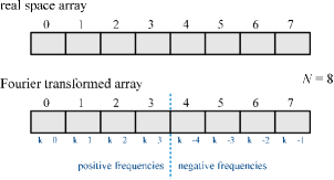

Figure 8: Commonly employed storage convention for DFTs. The positive frequencies are stored in the lower half of the array, the negative ones in the upper half.

Correspondingly, in 2D, the grid of real-space values is mapped to a grid of $k$-space values of the same dimensions. Again, negative frequencies seem to be stored ‘backwards’, with the smallest negative frequency having the largest linear index, and the most negative frequency appearing as first value past the middle of the mesh. But note that this is consistent with the translational invariance in $k$-space with respect to shifts of the indices by multiples of $N$.

7.5cm!

Figure 9: Sketch illustrating the implications of the reality constraint for the FFT of a field of reals in 2D. Different pairs of cells are related to each other as complex conjugate numbers (labeled as colored blocks), and some are aliased to themselves (orange) so that they end up being real.

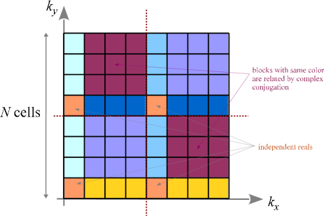
Finally, when we have a real real-space field (such as the physical density), the discrete Fourier transform fulfills a reality constraint of the form $\hat{\rho}_{\vec{k}}=\hat{\rho}_{-\vec{k}}^{\star}$. This implies a set of relations between the complex values that make up the Fourier transform of $\rho$, reducing the number of values that can be chosen arbitrarily. What does this imply in the discrete case? Consider the sketch shown in Fig. 9, in which regions of like color are related to each other by the reality constraint. Note that $k_{x}=N/2$ indices are aliased to themselves under complex conjugation, i.e. negating this gives $k_{x}={-N/2}$, but since $N$ can be added, this mode really maps again to $k_{x}=N/2$. Nevertheless, for the yellow regions there are always different partner cells when one considers the corresponding $-\vec{k}$ cell. Only for the orange cells this is not the case; those are mapped to themselves and are hence real due to the reality contraint.

If we now count how many independent numbers we have in the Fourier transformed grid of a 2D real field, we find

$$2\left(\frac{N}{2}-1\right)^{2}\times 2\;+\;4\left(\frac{N}{2}-1\right)\times 2\;+\;4\times 1.$$ (128)

The first term accounts for the two square-shaped regions that have different mirrored regions. Those contain $(\frac{N}{2}-1)^{2}$ complex numbers, each with two independent real and imaginary values. Then there are 4 different sections of rows and columns that are related to each other by mirroring in $k$-space. Those contain $(\frac{N}{2}-1)$ complex numbers each. Finally, there are 4 independent cells that are real and hence account for one independent value each. Reassuringly, the sum of equation (128) works out to $N^{2}$, which is the result we expect: the number of independent values in Fourier space must be exactly equal to the $N^{2}$ real values we started out with, otherwise we would not expect a strictly reversible transformation.

Non-periodic problems with ‘zero padding’

Can we use the FFT/DFT techniques discussed above also to calculate non-periodic force fields? At first, this may seem impossible since the DFT is intrinsically periodic. However, through the so-called zero-padding trick one can circumvent this limitation.

7.5cm!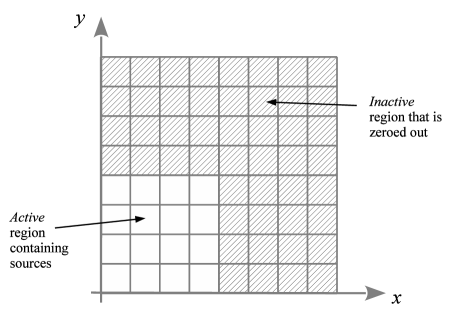

Figure 10: Sketch of zero padding used to treat non-periodic problems with the discrete Fourier transform.

Let’s discuss the procedure based on a 2D example (it works also in 1D or 3D, of course):

1. We need to arrange our mesh such that the source distribution lives only in one quarter of the mesh, the rest of the density field needs to be zeroed out. Schematically we hence have the situation depicted in Figure 10.

2. We now set up our desired real-space Green’s function, i.e. this is the response of a mass at the origin. The Green’s function for the whole mesh is set-up as $g_{N-i,j}=g_{i,N-j}=g_{N-i,N-j}=g_{i,j}$ where $0\leq i,j\leq N/2$. This is equivalent to defining $g$ everywhere on the mesh, and using as relevant distance the distance to the nearest periodic image of the origin. Note that by replicating $g$ with the condition of periodicity, the tessellated mesh then effectively yields a Green’s function that is nicely symmetric around the origin.

3. We now want to carry out the real-space convolution

   $$\phi=g\star\rho$$ (129)

   by using the definition of the discrete, periodic convolution

   $$\Phi_{\vec{p}}=\sum_{\vec{n}}g_{\vec{p}-\vec{n}}\,\rho_{\vec{n}},$$ (130)

   where both $g$ and $\rho$ are treated as periodic fields for which adding multiples of $N$ to the indices does not change anything. We see that this sum indeed yields the correct result for the non-periodic potential in the quarter of the mesh that contains our source distribution. This is because the Green’s function ‘sees’ only one copy of the source distribution in this sector; the zero-padded region is big enough to prevent any cross-talk from the (existing) periodic images of the source distribution. This is different in the other three quadrants of the mesh. Here we obtain incorrect potential values that are basically useless and need to be discarded.

4. Given that equation (130) yields the correct result in the region of the mesh covered by the sources, we may now just as well use periodic FFTs in the usual way to carry out this convolution quickly! A downside of this procedure is that it features an enlarged cost in terms of CPU and memory usage. Because we have to effectively double the mesh-size compared to the corresponding periodic problem, the cost goes up by a factor of 4 in 2D, and by a factor of 8 in 3D.

5. We note that James (1977) proposed an ingenious trick based that allows a more efficient treatment of isolated source distributions. Through suitably determined correction masses on the boundaries, the memory and cpu cost can be reduced compared to the zero-padding approach described above.

4.3 Multigrid techniques

Let’s return once more to the problem of solving Poisson’s equation,

$$\nabla^{2}\Phi=4\pi G\rho,$$ (131)

and consider first the one-dimensional problem, i.e.

$$\frac{\partial^{2}\Phi}{\partial x^{2}}=4\pi G\rho(x).$$ (132)

The spatial derivative on the left hand-side can be approximated as

$$\left(\frac{\partial^{2}\Phi}{\partial x^{2}}\right)_{i}\simeq\frac{\Phi_{i+1}-2\Phi_{i}+\Phi_{i-1}}{h^{2}},$$ (133)

where we have assumed that $\Phi$ is discretized with $N$ points on a regular mesh with spacing $h$, and $i$ is the cell index. This means that we have the equations

$$\frac{\Phi_{i+1}-2\Phi_{i}+\Phi_{i-1}}{h^{2}}=4\pi G\rho_{i}.$$ (134)

There are $N$ of these equations, for the $N$ unknowns $\Phi_{i}$, with $i\in\{0,1,\ldots,N-1\}$. This means we should in principle be able to solve this algebraically! In other words, the system of equations can be rewritten as a standard linear set of equations, in the form

$$\vec{A}\vec{x}=\vec{b},$$ (135)

with a vector of unknowns, $\vec{x}=(\Phi_{i})$, and a right hand side $\vec{b}=\frac{4\pi G}{h^{2}}\vec{\rho}$. In the 1D case, the matrix $\vec{A}$ (assuming periodic boundary conditions) is explicitly given as

$$\vec{A}=\left(\begin{array}[]{rrrrrr}-2&1&&&&1\\ 1&-2&1&&&\\ &1&-2&1&&\\ &&\ldots&&&\\ &&&1&-2&1\\ 1&&&&1&-2\\ \end{array}\right).$$ (136)

Solving equation (135) directly constitutes a matrix inversion that can in principle be carried out by LU-decomposition or Gauss elimination with pivoting (e.g. Press et al., 1992). However, the computational cost of these procedures is of order ${\cal O}(N^{3})$, meaning that it becomes extremely costly with growing $N$, and rather sooner than later infeasible, already for problems of small to moderate size.

Jacobi iteration

However, if we are satisfied with an approximate solution, then we can turn to iterative solvers that are much faster. Suppose we decompose the matrix $\vec{A}$ as

$$\vec{A}=\vec{D}-(\vec{L}+\vec{U}),$$ (137)

where $\vec{D}$ is the diagonal part, $\vec{L}$ is the (negative) lower diagonal part and $\vec{U}$ is the upper diagonal part. Then we have

$$\left[\vec{D}-(\vec{L}+\vec{U})\right]\vec{x}=\vec{b},$$ (138)

and from this

$$\vec{x}=\vec{D}^{-1}\vec{b}+\vec{D}^{-1}(\vec{L}+\vec{U})\vec{x}.$$ (139)

We can use this to define an iterative sequence of vectors $\vec{x}^{n}$:

$$\vec{x}^{(n+1)}=\vec{D}^{-1}\vec{b}+\vec{D}^{-1}(\vec{L}+\vec{U})\vec{x}^{(n)}.$$ (140)

This is called Jacobi iteration (e.g. Saad, 2003). Note that $\vec{D}^{-1}$ is trivially obtained because $\vec{D}$ is diagonal. i.e. here $(\vec{D}^{-1})_{ii}=1/\vec{A}_{ii}$.

The scheme converges if and only if the so-called convergence matrix

$$\vec{M}=\vec{D}^{-1}(\vec{L}+\vec{U})$$ (141)

has only eigenvalues that are less than 1, or in other words, that the spectral radius $\rho_{s}(\vec{M})$ fullfils

$$\rho_{s}(\vec{M})\equiv\max_{i}|\lambda_{i}|<1.$$ (142)

We can easily derive this condition by considering the error vector of the iteration. At step $n$ it is defined as

$$\vec{e}^{(n)}\equiv\vec{x}_{\rm exact}-\vec{x}^{(n)},$$ (143)

where $\vec{x}_{\rm exact}$ is the exact solution. We can use this to write the error at step $n+1$ of the iteration as

$$\vec{e}^{(n+1)}=\vec{x}_{\rm exact}-\vec{x}^{(n+1)}=\vec{x}_{\rm exact}-\vec{D}^{-1}\vec{b}-\vec{D}^{-1}(\vec{L}+\vec{U})\vec{x}^{(n)}=\vec{M}\vec{x}_{\rm exact}-\vec{M}\vec{x}^{(n)}=\vec{M}\vec{e}^{(n)}$$ (144)

Hence we find

$$\vec{e}^{(n)}=\vec{M}^{n}\vec{e}^{(0)}.$$ (145)

This implies $|\vec{e}^{(n)}|\leq[\rho_{s}(\vec{M})]^{n}|\vec{e}^{(0)}|$, and hence convergence if the spectral radius is smaller than 1.

For completeness, we state the Jacobi iteration rule for the Poisson equation in 3D when a simple 2-point stencil is used in each dimension for estimating the corresponding derivatives:

$$\Phi_{i,j,k}^{(n+1)} = \frac{1}{6}\left(\Phi_{i+1,j,k}+\Phi_{i-1,j,k}+\Phi_{i,j+1,k}+\Phi_{i,j-1,k}+\Phi_{i,j,k+1}+\Phi_{i,j,k-1}\right.$$ (146)

$$\left.-4\pi Gh^{2}\rho_{i,j,k}\right).$$

Gauss-Seidel iteration

The central idea of Gauss-Seidel iteration is to use the updated values as soon as they become available for computing further updated values. We can formalize this as follows. Adopting the same decomposition of $\vec{A}$ as before, we can write

$$(\vec{D}-\vec{L})\vec{x}=\vec{U}\vec{x}+\vec{b},$$ (147)

from which we obtain

$$\vec{x}=(\vec{D}-\vec{L})^{-1}\vec{U}\vec{x}+(\vec{D}-\vec{L})^{-1}\vec{b},$$ (148)

suggesting the iteration rule

$$\vec{x}^{(n+1)}=(\vec{D}-\vec{L})^{-1}\vec{U}\vec{x}^{(n)}+(\vec{D}-\vec{L})^{-1}\vec{b}.$$ (149)

This seems at first problematic, because we can’t easily compute $(\vec{D}-\vec{L})^{-1}$. But we can modify the last equation as follows:

$$\vec{D}\vec{x}^{(n+1)}=\vec{U}\vec{x}^{(n)}+\vec{L}\vec{x}^{(n+1)}+\vec{b}.$$ (150)

From which we get the alternative form:

$$\vec{x}^{(n+1)}=\vec{D}^{-1}\vec{U}\vec{x}^{(n)}+\vec{D}^{-1}\vec{L}\vec{x}^{(n+1)}+\vec{D}^{-1}\vec{b}.$$ (151)

Again, this may seem of little help because it looks like $\vec{x}^{(n+1)}$ would only be implicitly given. However, if we start computing the new elements in the first row $i=1$ of this matrix equation, we see that no values of $\vec{x}^{(n+1)}$ are actually needed, because $\vec{L}$ has only elements below the diagonal. For the same reason, if we then proceed with the second row $i=2$, then with $i=3$, etc., only elements of $\vec{x}^{(n+1)}$ from rows above the current one are needed. So we can calculate things in this order without problem and make use of the already updated values. It turns out that this speeds up the convergence quite a bit, with one Gauss-Seidel step often being close to two Jacobi steps.

Red black ordering

A problematic point about Gauss-Seidel is that the equations have to be solved in a specific sequential order, meaning that this part cannot be parallelized. Also, the result will in general depend on which element is selected to be the first. To overcome this problem, one can sometimes use so-called red-black ordering, which effectively is a compromise between Jacobi and Gauss-Seidel.

Certain update rules, such as that for the Poisson equation, allow a decomposition of the cells into disjoint sets whose update rules depend only on cells from other sets, as shown in Fig. 11. For example, for the Poisson equation, this is the case for a chess-board like pattern of ‘red’ and ‘black’ cells.

7.4cm!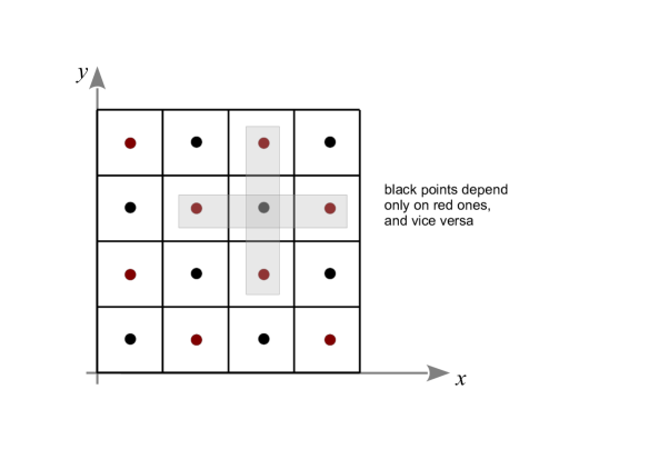

Figure 11: Red-black ordering in which two interleaved chessboard-like patterns are formed that can be independently processed with immediate updating.

One can then first update all the black points (which rely only on the red points), followed by an update of all the red points (which rely only on the black ones). In the second of these two half-steps, one can then use the updated values from the first half-step, making it intuitively clear why such a scheme can almost double the convergence rate relative to Jacobi.

The multigrid technique

Iterative solvers like Jacobi or Gauss-Seidel often converge quite slowly, in fact, the convergence seems to “stall” after a few steps and proceeds only anemically. One also observes that high-frequency errors in the solution are damped out quickly by the iterations, but long-wavelength errors die out much more slowly. Intuitively this is not unexpected: In every iteration, only neighboring points communicate, so the information “travels” only by one cell (or more generally, one stencil length) per iteration. And for convergence, it has to propagate back and forth over the whole domain a few times.

Idea By going to a coarser mesh, we may be able to compute an improved initial guess which may help to speed up the convergence on the fine grid (Brandt, 1977). Note that on the coarser mesh, the relaxation will be computationally cheaper (since there are only $1/8$ as many points in 3D, or $1/4$ in 2D), and the convergence rate should be faster, too, because the perturbation is there less smooth and effectively on a smaller scale relative to the coarser grid.

So schematically, we, for example, might imagine an iteration scheme where we first iterate the problem $\vec{A}\vec{x}=\vec{b}$ on a mesh with cells $4h$, i.e. for times coarser than the fine mesh. Once we have a solution there, we continue to iterate it on a mesh coarsened with cell size $2h$, and only finally we iterate to solution on the fine mesh with cell size $h$.

A couple of questions immediately come up when we want to work out the details of this basic idea:

1. How do we get from a coarse solution to a guess on a finer grid?

2. How should we solve $\vec{A}\vec{x}=\vec{b}$ on the coarsened mesh?

3. What if there is still an error left with long wavelength on the fine grid?

In order to make things work, we clearly need mappings from a finer grid to a coarser one, and vice versa. This is the most important issue to solve.

Prolongation and restriction operations

Coarse-to-fine This transition is an interpolation step, or in the language of multigrid methods (Briggs et al., 2000), it is called prolongation. Let $\vec{x}^{(h)}$ be a vector defined on a mesh $\Omega^{(h)}$ with $N$ cells and spacing $h$, covering our computational domain. Similarly, let $\vec{x}^{(2h)}$ be a vector living on a coarser mesh $\Omega^{(2h)}$ with twice the spacing and half as many points per dimension. We now define a linear interpolation operator $\vec{I}_{2h}^{h}$ that maps points from the coarser to the fine mesh, as follows:

$$\vec{I}_{2h}^{h}\,\vec{x}^{(2h)}=\vec{x}^{(h)}.$$ (152)

A simple realization of this operator in 2D would be the following:

$$\vec{I}_{2h}^{h}:\;\;\left.\begin{array}[]{ll}x^{(h)}_{2i}=x^{(2h)}_{i}&\\ &\mbox{for $0\leq i<\frac{N}{2}$}.\\ x^{(h)}_{2i+1}=\frac{1}{2}(x^{(2h)}_{i}+x^{(2h)}_{i+1})&\\ \end{array}\right.$$ (153)

Here, every second point is simply injected from the coarse to the fine mesh, and the intermediate points are linearly interpolated from the neighboring points, which here boils down to a simple arithmetic average.

Fine-to-coarse The converse mapping represents a smoothing operation, or a restriction in multigrid-language. We can define the restriction operator as

$$\vec{I}_{h}^{2h}\,\vec{x}^{(h)}=\vec{x}^{(2h)},$$ (154)

which hence takes a vector defined on the fine grid $\Omega^{(h)}$ to one that lives on the coarse grid $\Omega^{(2h)}$. Again, lets give a simple realization example in 2D:

$$\vec{I}_{h}^{2h}:\;\;x^{(2h)}_{i}=\frac{x^{(h)}_{2i-1}+2x^{(h)}_{2i}+x^{(h)}_{2i+1}}{4}\;\;\mbox{for $0\leq i<\frac{N}{2}$}.$$ (155)

Evidently, this is a smoothing operation with a simple 3-point stencil.

One usually chooses these two operators such that the transpose of one is proportional to the other, i.e. they are related as follows:

$$\vec{I}_{h}^{2h}=c\,[\vec{I}_{2h}^{h}]^{\rm T},$$ (156)

where $c$ is a real number.

In a shorter notation, the above prolongation operator can be written as

$$\mbox{1D-prolongation,}\;\;\vec{I}_{2h}^{h}:\;\;\left]\;\frac{1}{2}\;\;1\;\;\frac{1}{2}\;\right[,$$ (157)

which means that every coarse point is added with these weights to three points of the fine grid. The fine-grid points accessed with weight $1/2$ will get contributions from two coarse grid points. Similarly, the restriction operator can be written with the short-hand notation

$$\mbox{1D-restriction,}\;\;\vec{I}_{h}^{2h}:\;\;\left[\;\frac{1}{4}\;\;\frac{1}{2}\;\;\frac{1}{4}\;\right].$$ (158)

This expresses that every coarse grid point is a weighted sum of three fine grid points.

For reference, we also state the corresponding low-order prolongation and restriction operators in 2D:

$$\mbox{2D-prolongation,}\;\;\vec{I}_{2h}^{h}: \;\;\left]\begin{array}[]{ccc}\frac{1}{4}&\frac{1}{2}&\frac{1}{4}\\ \\ \frac{1}{2}&1&\frac{1}{2}\\ \\ \frac{1}{4}&\frac{1}{2}&\frac{1}{4}\\ \end{array}\right[$$ (164)

$$\mbox{2D-restriction,}\;\;\vec{I}_{h}^{2h}: \;\;\left[\begin{array}[]{ccc}\frac{1}{16}&\frac{1}{8}&\frac{1}{16}\\ \\ \frac{1}{8}&\frac{1}{4}&\frac{1}{8}\\ \\ \frac{1}{16}&\frac{1}{8}&\frac{1}{16}\\ \end{array}\right]$$ (170)

Corresponding extensions to 3D can be readily derived.

The multigrid V-cycle

An important role in the multigrid approach plays the error vector, defined as

$$\vec{e}\equiv\vec{x}_{\rm exact}-\tilde{\vec{x}},$$ (171)

where $\vec{x}_{\rm exact}$ is the exact solution, and $\tilde{\vec{x}}$ the (current) approximate solution. Another important concept is the residual, defined as

$$\vec{r}\equiv\vec{b}-\vec{A}\tilde{\vec{x}}.$$ (172)

Note that the pair of error and residual are solutions of the original linear system, i.e. we have

$$\vec{A}\vec{e}=\vec{r}.$$ (173)

Coarse-grid correction scheme We now define a function that is supposed to return an improved solution $\tilde{\vec{x}}^{\prime(h)}$ for the problem $\vec{A}^{(h)}\vec{x}^{(h)}=\vec{b}^{(h)}$ on grid level $h$, based on some starting guess $\tilde{\vec{x}}^{(h)}$ and a right hand side $\vec{b}^{(h)}$. This so-called coarse grid correction,

$$\tilde{\vec{x}}^{\prime(h)}={\rm CG}(\tilde{\vec{x}}^{(h)},\vec{b}^{(h)}),$$ (174)

proceeds along the following steps:

1. Carry out a relaxation step on $h$ (for example by using one Gauss-Seidel or one Jacobi iteration).

2. Compute the residual: $\vec{r}^{(h)}=\vec{b}^{(h)}-\vec{A}^{(h)}\tilde{\vec{x}}^{(h)}$.

3. Restrict the residual to a coarser mesh: $\vec{r}^{(2h)}=\vec{I}_{h}^{2h}\,\vec{r}^{(h)}$.

4. Solve $\vec{A}^{(2h)}\vec{e}^{(2h)}=\vec{r}^{(2h)}$ on the coarsened mesh, with $\tilde{\vec{e}}^{(2h)}=0$ as initial guess.

5. Prolong the obtained error $\vec{e}^{(2h)}$ to the finer mesh, $\vec{e}^{(h)}=\vec{I}_{2h}^{h}\,\vec{e}^{(2h)}$, and use it to correct the current solution on the fine grid: $\tilde{\vec{x}}^{\prime(h)}=\tilde{\vec{x}}^{(h)}+\vec{e}^{(h)}$.

6. Carry out a further relaxation step on the fine mesh $h$.

How do we carry out step 4 in this scheme? We can use recursion! Because what we have to do in step 4 is exactly the job description of the function ${\rm CG}(.,.)$. However, we also need a stopping condition for the recursion, which is simply a prescription that tells us under which conditions we should skip steps 2 to 5 in the above scheme. We can do this by simply saying that further coarsening of the problem should stop once we have reached a minimum number of cells $N$. At this point we either just do the relaxation steps, or we solve the remaining problem exactly.

7.5cm!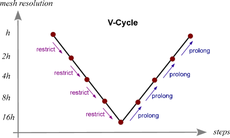

Figure 12: The typical V-cycle of a multigrid iteration scheme. The current solution on a fine mesh is recursively restricted to coarser meshes. Coarse-grid corrections are then prolonged back up to the finer meshes, interleaved with one Gauss-Seidl or Jacobi iteration at the corresponding mesh level.

V-Cycle When the coarse grid correction scheme is recursively called, we arrive at the schematic diagram shown in Fig. 12 for how the iteration progresses, which is called a V-cycle. It turns out that the V-cycle rather dramatically speeds up the convergence rate of simple iterative solvers for linear systems of equations. It is easy to show that the computational cost of one V-cycle is of order ${\cal O}(N_{\rm grid})$, where $N_{\rm grid}$ is the number of grid cells on the fine mesh. A convergence to truncation error (i.e. machine precision) requires several V-cycles and involves a computational cost of order ${\cal O}(N_{\rm grid}\log N_{\rm grid})$. For the Poisson equation, this is the same cost scaling as one gets with FFT-based methods. In practice, good implementations of the two schemes should roughly be equally fast. In cosmology, a multigrid solver is for example used by the MLAPM (Knebe et al., 2001) and RAMSES codes (Teyssier, 2002). An interesting advantage of multigrid is that it requires less data communication when parallelized on distributed memory machines.

One problem we haven’t addressed yet is how one finds the operator $\vec{A}^{(2h)}$ required on the coarse mesh. The two most commonly used options for this are:

• Direct coarse grid approximation: Here one simply uses the same discrete equations on the coarse grid as on the fine grid, just scaled by the grid resolution $h$ as needed. In this case, the stencil of the matrix does not change.

• Galerkin coarse grid approximation: Here one defines the coarse operator as

  $$\vec{A}^{(2h)}=\vec{I}_{h}^{2h}\,\vec{A}^{(h)}\,\vec{I}_{2h}^{h},$$ (175)

  which is formally the most consistent way of defining $\vec{A}^{(2h)}$, and in this sense optimal. However, computing the matrix in this way can be a bit cumbersome, and it may involve a growing size of the stencil, which then leads to an enlarged computational cost.

The full multigrid method

The V-cycle scheme discussed thus far still relies on an initial guess for the solution, and if this guess is bad, one has to do more V-cycles to reach satisfactory convergence. This raises the question on how one may get a good guess. If one is dealing with the task of repeatedly having to solve the same problem over and over again with only small changes from solution to solution (as will often be the case in dynamical simulation problems) one may be able to simply use the solution from the previous timestep as a guess. In all other cases, one can allude to the following idea: Let’s get a good guess by solving the problem on a coarser grid first, and then interpolate the coarse solution to the fine grid as a starting guess.

7.5cm!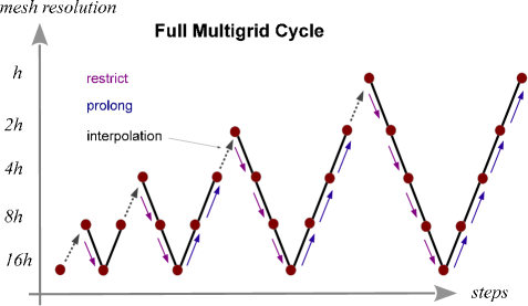

Figure 13: The full multigrid cycle in which also the problem of finding an adequate starting guess is addressed.

But at the coarser grid, one is then again confronted with the task to solve the problem without a starting guess. Well, we can simply recursively apply the idea again, and delegate the finding of a good guess to a yet coarser grid, etc. This then yields the full multigrid cycle, as depicted in Fig. 13. It involves the following steps:

1. Initialize the right hand side on all grid levels, $\vec{b}^{(h)}$, $\vec{b}^{(2h)}$, $\vec{b}^{(4h)}$, $\ldots$, $\vec{b}^{(H)}$, down to some coarsest level $H$.

2. Solve the problem (exactly) on the coarsest level $H$.

3. Given a solution on level $i$ with spacing $2h$, map it to the next level $i+1$ with spacing $h$ and obtain the initial guess $\tilde{\vec{x}}^{(h)}=I_{2h}^{h}\,\vec{x}^{(2h)}$.

4. Use this starting guess to solve the problem on the level $i+1$ with one V-cycle.

5. Repeat Step 3 until the finest level is reached.

The computational cost of such a full multigrid cycle is still of order the number of mesh cells, as before.

4.4 Hierarchical multipole methods (“tree codes”)

Another approach for a real-space evaluation of the gravitational field are so-called tree codes (Barnes & Hut, 1986). In cosmology, they are for example used in the PKDGRAV/GASOLINE (Wadsley et al., 2004) and GADGET (Springel et al., 2001; Springel, 2005) codes.

Multipole expansion

The central idea is here to use the multipole expansion of a distant group of particle to describe its gravity, instead of summing up the forces from all individual particles.

5.5cm!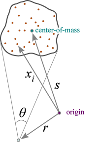

Figure 14: Multipole expansion for a group of distant particles. Provided the reference point $\vec{r}$ is sufficiently far away, the particles are seen under a small opening angle $\theta$, and the field created by the particle group can be approximated by the monopole term at its center of mass, augmented with higher order multipole corrections if desired.

The potential of the group is given by

$$\Phi(\vec{r})=-G\sum_{i}\frac{m_{i}}{|\vec{r}-\vec{x}_{i}|},$$ (176)

which we can re-write as

$$\Phi(\vec{r})=-G\sum_{i}\frac{m_{i}}{|\vec{r}-\vec{s}+\vec{s}-\vec{x}_{i}|}.$$ (177)

Now we expand the denominator assuming $|\vec{x}_{i}-\vec{s}|\ll|\vec{r}-\vec{s}|$, which will be the case provided the opening angle $\theta$ under which the group is seen is sufficiently small, as sketched in Figure 14. We can then use the Taylor expansion

$$\frac{1}{|\vec{y}+\vec{s}-\vec{x}_{i}|}=\frac{1}{|\vec{y}|}-\frac{\vec{y}\cdot(\vec{s}-\vec{x}_{i})}{|\vec{y}|^{3}}+\frac{1}{2}\frac{\vec{y}^{T}\left[3(\vec{s}-\vec{x}_{i})(\vec{s}-\vec{x}_{i})^{T}-(\vec{s}-\vec{x}_{i})^{2}\right]\vec{y}}{|\vec{y}|^{5}}+\ldots,$$ (178)

where we introduced $\vec{y}\equiv\vec{r}-\vec{s}$ as a short-cut. The first term on the right hand side gives rise to the monopole moment, the second to the dipole moment, and the third to the quadrupole moment. If desired, one can continue the expansion to ever higher order terms.

These multipole moments then become properties of the group of particles:

$$\mbox{monopole:}\;\;\;M=\sum_{i}m_{i},$$ (179)

$$\mbox{quadrupole:}\;\;\;Q_{ij}=\sum_{k}m_{k}\left[3(\vec{s}-\vec{x}_{k})_{i}(\vec{s}-\vec{x}_{k})_{j}-\delta_{ij}(\vec{s}-\vec{x}_{k})^{2}\right].$$ (180)

The dipole vanishes, because we carried out the expansion relative to the center-of-mass, defined as

$$\vec{s}=\frac{1}{M}\sum_{i}m_{i}\vec{x}_{i}.$$ (181)

If we restrict ourselves to terms of up to quadrupole order, we hence arrive at the expansion

$$\Phi(\vec{r})=-G\left(\frac{M}{|\vec{y}|}+\frac{1}{2}\frac{\vec{y}^{T}\vec{Q}\vec{y}}{|\vec{y}|^{5}}\right),\;\;\;\;\;\;\vec{y}=\vec{r}-\vec{s},$$ (182)

from which also the force can be readily obtained through differentiation. Recall that we expect the expansion to be accurate if

$$\theta\simeq\frac{\left<|\vec{x}_{i}-\vec{s}|\right>}{|\vec{y}|}\simeq\frac{l}{y}\ll 1,$$ (183)

where $l$ is the radius of the group.

Hierarchical grouping

Tree algorithms are based on a hierarchical grouping of the particles, and for each group, one then pre-computes the multipole moments for later use in approximations of the force due to distant groups. Usually, the hierarchy of groups is organized with the help of a tree-like data structure, hence the name “tree algorithms”.

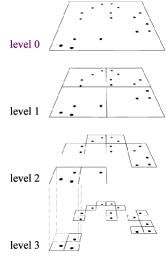
There are different strategies for defining the groups. In the popular Barnes & Hut (1986) oct-tree, one starts out with a cube that contains all the particles. This cube is then subdivided into 8 sub-cubes of half the size in each spatial dimension. One continues with this refinement recursively until each subnode contains only a single particle. Empty nodes (sub-cubes) need not be stored. Figure 15 shows a schematic sketch how this can look like in two dimensions.

b]

Figure 15: Organization of the Barnes & Hut (1986) tree in two dimensions (quad tree). All particles are enclosed in a square-shaped box. This is then hierarchically subdivided until each particle finds itself in a node on its own. Empty cells do not need to be stored.

• We note that the oct-tree is not the only possible grouping strategy. Sometimes kd-trees (Stadel, 2001), or binary trees where subdivisions are done along alternating spatial axes are used.

• An important property of such hierarchical, tree-based groupings is that they are geometrically highly flexible and adjust to any clustering state the particles may have. They are hence automatically adaptive.

• Also, there is no significant slow-down when severe clustering starts.

• The simplest way to construct the hierarchical grouping is to sequentially insert particles into the tree, and then to compute the multipole moments recursively.

Tree walk

The force calculation with the tree then proceeds by walking the tree. Starting at the root node, one checks for every node whether the opening angle under which it is seen is smaller than a prescribed tolerance angle $\theta_{c}$. If this is the case, the multipole expansion of the node can be accepted, and the corresponding partial force is evaluated and added to an accumulation of the total force. The tree walk along this branch of the tree can then be stopped. Otherwise, one must open the tree node and consider all its sub-nodes in turn.

The resulting force is approximate by construction, but the overall size of the error can be conveniently controlled by the tolerance opening angle $\theta_{c}$ (see also Salmon & Warren, 1994). If one makes this smaller, more nodes will have to be opened. This will make the residual force errors smaller, but at the price of a higher computational cost. In the limit of $\theta_{c}\to 0$ one gets back to the expensive direct summation force.

An interesting variant of this approach to walk the tree is obtained by not only expanding the potential on the source side into a multipole expansion, but also around the target coordinate. This can yield a substantial additional acceleration and results in so-called fast multipole methods (FFM). The FALCON code of Dehnen (2000, 2002) employs this approach. A further advantage of the FFM formulation is that force anti-symmetry is manifest, so that momentum conservation to machine precision can be achieved. Unfortunately, the speed advantages of FFM compared to ordinary tree codes are significantly alleviated once individual time-step schemes are considered. Also, FFM is more difficult to parallelize efficiently on distributed memory machines.

Cost of the tree-based force computations

How do we expect the total cost of the tree algorithm to scale with particle number $N$? For simplicity, let’s consider a sphere of size $R$ containing $N$ particles that are approximately homogeneously distributed. The mean particle spacing of these particles will then be

$$d=\left[\frac{(4\pi/3)R^{3}}{N}\right]^{1/3}.$$ (184)

We now want to estimate the number of nodes that we need for calculating the force on a central particle in the middle of the sphere. We can identify the computational cost with the number of interaction terms that are needed. Since the used nodes must tessellate the sphere, their number can be estimated as

$$N_{\rm nodes}=\int_{d}^{R}\frac{4\pi r^{2}\,{\rm d}r}{l^{3}(r)},$$ (185)

where $l(r)$ is the expected node size at distance $r$, and $d$ is the characteristic distance of the nearest particle. Since we expect the nodes to be close to their maximum allowed size, we can set $l\simeq\theta_{c}r$. We then obtain

$$N_{\rm nodes}=\frac{4\pi}{\theta_{c}^{3}}\ln\frac{R}{d}\propto\frac{\ln N}{\theta_{c}^{3}}.$$ (186)

The total computational cost for a calculation of the forces for all particles is therefore expected to scale as ${\cal O}(N\ln N)$. This is a very significant improvement compared with the $N^{2}$-scaling of direct summation.

We may also try to estimate the expected typical force errors. If we keep only monopoles, the error in the force per unit mass from one node should roughly be of order the truncation error, i.e. about

$$\Delta F_{\rm node}\sim\frac{GM_{\rm node}}{r^{2}}\theta^{2}.$$ (187)

The errors from multipole nodes will add up in quadrature, hence

$$(\Delta F_{\rm tot})^{2}\sim N_{\rm node}(\Delta F_{\rm node})^{2}=N_{\rm node}\left(\frac{GM_{\rm node}}{r^{2}}\theta^{2}\right)^{2}\propto\frac{\theta^{4}}{N_{\rm node}}\propto\theta^{7}.$$ (188)

The force error for a monopoles-only scheme therefore scales as $(\Delta F_{\rm tot})\propto\theta^{3.5}$, roughly inversely as the invested computational cost. A much more detailed analysis of the performance characteristics of tree codes can be found, for example, in Hernquist (1987).

4.5 TreePM schemes

While the high adaptivity of tree algorithms is particularly ideal for strongly clustered particle distributions and when a high spatial force accuracy is desired, the mesh-based approaches are usually faster when only a coarsely resolved gravitational field on large scales is required. In particular, the particle-mesh (PM) approach based on Fourier techniques is probably the fastest method to calculate the gravitational field on a homogenous mesh. The obvious limitation of this method is however that the force resolution cannot be better than the size of one mesh cell, and the latter cannot be easily made small enough to resolve all the scales of interest in cosmological simulations.

One interesting idea is to try to combine both approaches into a unified scheme, where the gravitational field on large scales is calculated with a PM algorithm, while the short-range forces are delivered by a hierarchical tree method. Such TreePM schemes have first been proposed by Xu (1995) and Bagla (2002), and a version similar to that of Bagla (2002) is implemented in the GADGET2 code (Springel, 2005).

In order to achieve a clean separation of scales, one can consider the potential in Fourier space. The individual modes $\Phi_{\vec{k}}$ can be decomposed into a long-range and a short-range part, as follows:

$$\Phi_{\vec{k}}=\Phi^{{\rm long}}_{\vec{k}}+\Phi^{{\rm short}}_{\vec{k}},$$ (189)

where

$$\Phi^{{\rm long}}_{\vec{k}}=\Phi_{\vec{k}}\exp(-\vec{k}^{2}r_{s}^{2}),$$ (190)

and

$$\Phi^{{\rm short}}_{\vec{k}}=\Phi_{\vec{k}}[1-\exp(-\vec{k}^{2}r_{s}^{2})],$$ (191)

with $r_{s}$ describing the spatial scale of the force-split. Due to the exponential cut-off of the Fourier-spectrum of the long-range force, a PM grid of finite size can be used to fully resolve this force component (this is achieved once the cell size is a few times smaller than $r_{s}$). Compared to the ordinary PM-scheme, the only change is that the Greens function in Fourier-space gets an additional exponential smoothing factor. Thanks to this force-shaping factor, inaccuracies such as force anisotropies from the mesh geometry can be made arbitrarily small, so that the long-range force in the transition region between the force components is accurately computed by the PM scheme.

To calculate the short-range force, one transforms equation (191) back to real space. Assuming a single point mass $m$ somewhere in a periodic box of size $L$, this becomes for $r_{s}\ll L$:

$$\Phi^{{\rm short}}(\vec{x})=-G\frac{m}{r}{\rm erfc}\left(\frac{r}{2r_{s}}\right),$$ (192)

where $r=\min(|\vec{x}-\vec{r}-\vec{n}L|)$ is defined as the smallest distance of any of the periodic images ($\vec{n}$ is an arbitrary integer triplet) of the point mass at $\vec{r}$ relative to the point $\vec{x}$. Now, this is recognized as the ordinary Newtonian potential, modified with a truncation factor that rapidly turns off the force at a finite distance of order $r_{s}$. In fact, the force drops to about 1% of its Newtonian value for $r\simeq 4.5r_{s}$, and quickly becomes completely negligible at still larger separations.

The potential (192) can still be treated with a hierarchical tree algorithm, except for the simplification that any tree node more distant than a finite cut-off range (of order $\sim 5r_{s}$) can be immediately discarded in the tree walk. This can yield a significant speed-up relative to a plain tree code, because the tree-walk can now be restricted to a small region around the target particle as opposed to having to be carried out for the full volume. Also, periodic boundary conditions do not have to be included explicitly through Ewald summation (Hernquist et al., 1991) any more, rather they are absorbed in the periodic PM force. Another advantage is that for close to homogeneous particle distributions, the PM method used for long-range forces delivers a precise force quickly, whereas a pure tree code struggles in this regime to reach the required force accuracy, simply because here large forces in all directions, which almost completely compensate in the end, need to be evaluated with high relative accuracy, otherwise they do not cancel out properly. Finally, the hybrid TreePM scheme also offers the possibility to split the time integration into a less frequent evaluation of the long-range force, and a more frequent evaluation of the short-range tree force, because the former is associated with longer dynamical time scales than the latter. This can be exploited to realize additional efficiency gains, and can in principle even be done in a symplectic fashion (Saha & Tremaine, 1992; Springel, 2005).

5 Basic gas dynamics

Gravity is the dominant driver behind cosmic structure formation (e.g. Mo et al., 2010), but at small scales hydrodynamics in the baryonic components becomes very important, too. In this section we very briefly review the basic equations and some prominent phenomena related to gas dynamics in order to make the discussion of the numerical fluid solvers used in galaxy evolution more accessible. For a detailed introduction to hydrodynamics, the reader is referred to the standard textbooks on this subject (e.g. Landau & Lifshitz, 1959; Shu, 1992).

5.1 Euler and Navier-Stokes equations

The gas flows in astrophysics are often of extremely low density, making internal friction in the gas extremely small. In the limit of assuming internal friction to be completely absent, we arrive at the so-called ideal gas dynamics as described by the Euler equations. Most calculations in cosmology and galaxy formation are carried out under this assumption. However, in certain regimes, viscosity may still become important (for example in the very hot plasma of rich galaxy clusters), hence we shall also briefly discuss the hydrodynamical equations in the presence of physical viscosity, the Navier-Stokes equations, which in a sense describe real fluids as opposed to ideal ones. Phenomena such as fluid instabilities or turbulence are also best understood if one does not neglect viscosity completely.

Euler equations

If internal friction in a gas flow can be neglected, the dynamics of the fluid is governed by the Euler equations:

$$\frac{\partial\rho}{\partial t}+\nabla(\rho\vec{v})=0,$$ (193)

$$\frac{\partial}{\partial t}(\rho\vec{v})+\nabla(\rho\vec{v}\vec{v}^{T}+P)=0,$$ (194)

$$\frac{\partial}{\partial t}(\rho e)+\nabla[(\rho e+P)\vec{v}]=0,$$ (195)

where $e=u+\vec{v}^{2}/2$ is the total energy per unit mass, and $u$ is the thermal energy per unit mass. Each of these equations is a continuity law, one for the mass, one for the momentum, and one for the total energy. The equations hence form a set of hyperbolic conservation laws. In the form given above, they are not yet complete, however. One still needs a further expression that gives the pressure in terms of the other thermodynamic variables. For an ideal gas, the pressure law is

$$P=(\gamma-1)\rho u,$$ (196)

where $\gamma=c_{p}/c_{v}$ is the ratio of specific heats. For a monoatomic gas, we have $\gamma=5/3$.

Navier-Stokes equations

Real fluids have internal stresses, due to viscosity. The effect of viscosity is to dissipate relative motions of the fluid into heat. The Navier-Stokes equations are then given by

$$\frac{\partial\rho}{\partial t}+\nabla(\rho\vec{v})=0,$$ (197)

$$\frac{\partial}{\partial t}(\rho\vec{v})+\nabla(\rho\vec{v}\vec{v}^{T}+P)=\nabla\,\vec{\rm\Pi},$$ (198)

$$\frac{\partial}{\partial t}(\rho e)+\nabla[(\rho e+P)\vec{v}]=\nabla(\vec{\rm\Pi}\vec{v}).$$ (199)

Here $\vec{\rm\Pi}$ is the so-called viscous stress tensor, which is a material property. For $\vec{\rm\Pi}=0$, the Euler equations are recovered. To first order, the viscous stress tensor must be a linear function of the velocity derivatives (Landau & Lifshitz, 1959). The most general tensor of rank-2 of this type can be written as

$$\vec{\rm\Pi}=\eta\left[\nabla\vec{v}+(\nabla\vec{v})^{T}-\frac{2}{3}(\nabla\cdot\vec{v})\vec{1}\right]+\xi(\nabla\cdot\vec{v})\vec{1},$$ (200)

where $\vec{1}$ is the unit matrix. Here $\eta$ scales the traceless part of the tensor and describes the shear viscosity. $\xi$ gives the strength of the diagonal part, and is the so-called bulk viscosity. Note that $\eta$ and $\xi$ can in principle be functions of local fluid properties, such as $\rho$, $T$, etc.

Incompressible fluids In the following we shall assume constant viscosity coefficients. Also, we specialize to incompressible fluids with $\nabla\cdot\vec{v}=0$, which is a particularly important case in practice. Let’s see how the Navier-Stokes equations simplify in this case. Obviously, $\xi$ is then unimportant and we only need to deal with shear viscosity. Now, let us consider one of the components of the viscous shear force described by equation (198):

$$\frac{1}{\eta}(\nabla\,\vec{\rm\Pi})_{x} = \frac{\partial}{\partial x}\left(2\frac{\partial v_{x}}{\partial x}\right)+\frac{\partial}{\partial y}\left(\frac{\partial v_{x}}{\partial y}+\frac{\partial v_{y}}{\partial x}\right)+\frac{\partial}{\partial z}\left(\frac{\partial v_{x}}{\partial z}+\frac{\partial v_{z}}{\partial x}\right)$$ (201)

$$= \left(\frac{\partial^{2}}{\partial x^{2}}+\frac{\partial^{2}}{\partial y^{2}}+\frac{\partial^{2}}{\partial z^{2}}\right)v_{x}=\nabla^{2}v_{x},$$

where we made use of the $\nabla\cdot\vec{v}=0$ constraint. If we furthermore introduce the kinematic viscosity $\nu$ as

$$\nu\equiv\frac{\eta}{\rho},$$ (202)

we can write the equivalent of equation (198) in the compact form

$$\frac{{\rm D}\,\vec{v}}{{\rm D}\,t}=-\frac{\nabla P}{\rho}+\nu\nabla^{2}\vec{v},$$ (203)

where the derivative on the left-hand side is the Lagrangian derivative,

$$\frac{{\rm D}}{{\rm D}\,t}=\frac{\partial}{\partial t}+\vec{v}\cdot\nabla.$$ (204)

We hence see that the motion of individual fluid elements responds to pressure gradients and to viscous forces. The form (203) of the equation is also often simply referred to as the Navier-Stokes equation.

Scaling properties of viscous flows

Consider the Navier-Stokes equations for some flow problem that is characterized by some characteristic length $L_{0}$, velocity $V_{0}$, and density scale $\rho_{0}$. We can then define dimensionless fluid variables of the form

$$\hat{\vec{v}}=\frac{\vec{v}}{V_{0}},\;\;\;\;\;\;\;\;\;\;\;\;\hat{\vec{x}}=\frac{\vec{x}}{L_{0}},\;\;\;\;\;\;\;\;\;\;\;\;\hat{P}=\frac{P}{\rho_{0}V_{0}^{2}}.$$ (205)

Similarly, we define a dimensionless time, a dimensionless density, and a dimensionless Nabla operator:

$$\hat{t}=\frac{t}{L_{0}/V_{0}},\;\;\;\;\;\;\;\;\;\;\;\;\hat{\rho}=\frac{\rho}{\rho_{0}},\;\;\;\;\;\;\;\;\;\;\;\;\hat{\nabla}=L_{0}\nabla.\;\;\;\;\;\;\;\;\;\;\;\;$$ (206)

Inserting these definitions into the Navier-Stokes equation (203), we obtain the dimensionless equation

$$\frac{D\hat{\vec{v}}}{D\hat{t}}=-\frac{\hat{\nabla}\hat{P}}{\hat{\rho}}+\frac{\nu}{L_{0}V_{0}}\,\hat{\nabla}^{2}\hat{\vec{v}}.$$ (207)

Interestingly, this equation involves one number,

$${\rm Re}\equiv\frac{L_{0}V_{0}}{\nu},$$ (208)

which characterizes the flow and determines the structure of the possible solutions of the equation. This is the so-called Reynolds number. Problems which have similar Reynolds number are expected to exhibit very similar fluid behavior. One then has Reynolds-number similarity. In contrast, the Euler equations (${\rm Re}\to\infty$) exhibit always scale similarity because they are invariant under scale transformations.

One intuitive interpretation one can give the Reynolds number is that it measures the importance of inertia relative to viscous forces. Hence:

$${\rm Re}\approx\frac{\mbox{inertial forces}}{\mbox{viscous forces}}\approx\frac{D\vec{v}/Dt}{\nu\nabla^{2}\vec{v}}\approx\frac{V_{0}/(L_{0}/V_{0})}{\nu V_{0}/L_{0}^{2}}=\frac{L_{0}V_{0}}{\nu}.$$ (209)

If we have ${\rm Re}\sim 1$, we are completely dominated by viscosity. On the other hand, for ${\rm Re}\to\infty$ viscosity becomes unimportant and we approach an ideal gas.

5.2 Shocks

An important feature of hydrodynamical flows is that they can develop shock waves in which the density, velocity, temperature and specific entropy jump by finite amounts (e.g. Toro, 1997). In the case of the Euler equations, such shocks are true mathematical discontinuities. Interestingly, shocks can occur even from perfectly smooth initial conditions, which is a typical feature of hyperbolic partial differential equations. In fact, acoustic waves with sufficiently large amplitude will suffer from wave-steeping (because the slightly hotter wave crests travel faster than the colder troughs), leading eventually to shocks. Of larger practical importance in astrophysics are however the shocks that occur when flows collide supersonically; here kinetic energy is irreversibly transferred into thermal energy, a process that also manifests itself with an increase in entropy.

In the limit of vanishing viscosity (i.e. for the Euler equations), the differential form of the fluid equations breaks down at the discontinuity of a shock, but the integral form (the weak formulation) remains valid. In other words this means that the flux of mass, momentum and energy must remain continuous at a shock front. Assuming that the shock connects two piecewise constant states, this leads to the Rankine-Hugoniot jump conditions (Rankine, 1870). If we select a frame of reference where the shock is stationary ($v_{s}=0$) and denote the pre-shock state with $(v_{1},P_{1},\rho_{1})$, and the post-shock state as $(v_{2},P_{2},\rho_{2})$ (hence $v_{1},v_{2}>0$), we have

$$\rho_{1}v_{2}=\rho_{2}v_{2},$$ (210)

$$\rho_{1}v_{1}^{2}+P_{1}=\rho_{2}v_{2}^{2}+P_{2},$$ (211)

$$(\rho_{1}e_{1}+P_{1})v_{1}=(\rho_{2}e_{2}+P_{2})v_{2}.$$ (212)

For an ideal gas, the presence of a shock requires that the pre-shock gas streams supersonically into the discontinuity, i.e. $v_{1}>c_{1}$, where $c_{1}^{2}=\gamma\,P_{1}/\rho_{1}$ is the sound speed in the pre-shock phase. The Mach number

$${\cal M}=\frac{v_{1}}{c_{1}}$$ (213)

measures the strength of the shock (${\cal M}>1$). The shock itself decelerates the fluid and compresses it, so that we have $v_{2}<v_{1}$ and $\rho_{2}>\rho_{1}$. It also heats it up, so that $T_{2}>T_{1}$, and makes the postshock flow subsonic, with $v_{2}/c_{2}<1$. Manipulating equations (210) to (212), we can express the relative jumps in the thermodynamic quantities (density, temperature, entropy, etc.) through the Mach number alone, for example:

$$\frac{\rho_{2}}{\rho_{1}}=\frac{(\gamma+1){\cal M}^{2}}{(\gamma-1){\cal M}^{2}+2}.$$ (214)

5.3 Fluid instabilities

In many situations, gaseous flows can be subject to fluid instabilities in which small perturbations can rapidly grow, thereby tapping a source of free energy. An important example of this are Kelvin-Helmholtz and Rayleigh-Taylor instabilities, which we briefly discuss in this subsection.

6.5cm!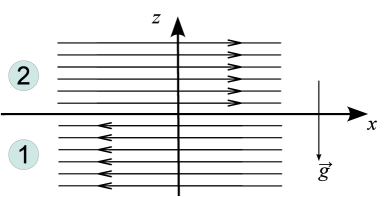

Figure 16: Geometry of a generic shear flow.

Stability of a shear flow We consider a flow in the $x$-direction, which in the lower half-space $z<0$ has velocity $U_{1}$ and density $\rho_{1}$, whereas in the upper half-space the gas streams with $U_{2}$ and has density $\rho_{2}$. In addition there can be a homogeneous gravitational field $\vec{g}$ pointing into the negative $z$-direction, as sketched in Figure 16.

The stability of the flow can be analysed through perturbation theory. To this end, one can for example treat the flow as an incompressible potential flow, and carry out an Eigenmode analysis in Fourier space. With the help of Bernoulli’s theorem one can then derive an equation for a function $\xi(x,t)=z$ that describes the $z$-location of the interface between the two phases of the fluid. Details of this calculation can for example be found in Pringle & King (2007). For a single perturbative Fourier mode

$$\xi = \hat{\xi}\exp[i(kx-\omega t)],$$ (215)

one then finds that non-trivial solutions with $\hat{\xi}\neq 0$ are possible for

$$\omega^{2}(\rho_{1}+\rho 2)-2\omega k(\rho_{1}U_{1}+\rho_{2}U_{2})+k^{2}(\rho_{1}U_{1}^{2}+\rho_{2}U_{2}^{2})+(\rho_{2}-\rho 1)kg=0,$$ (216)

which is the dispersion relation. Unstable, exponentially growing mode solutions appear if there are solutions for $\omega$ with positive imaginary part. Below, we examine the dispersion relation for a few special cases.

Rayleigh-Taylor instability Let us consider the case of a fluid at rest, $U_{1}=U_{2}=0$. The dispersion relation simplifies to

$$\omega^{2}=\frac{(\rho_{1}-\rho_{2})kg}{\rho_{1}+\rho_{2}}.$$ (217)

We see that for $\rho_{2}>\rho_{1}$, i.e. the denser fluid lies on top, unstable solutions with $\omega^{2}<0$ exist. This is the so-called Rayleigh-Taylor instability. It is in essence buoyancy driven and leads to the rise of lighter material underneath heavier fluid in a stratified atmosphere, as illustrated in the simulation shown in Figure 17. The free energy that is tapped here is the potential energy in the gravitational field. Also notice that for an ideal gas, arbitrary small wavelengths are unstable, and those modes will grow fastest. If on the other hand we have $\rho_{1}>\rho_{2}$, then the interface is stable and will only oscillate when perturbed.

Figure 17: A growing Rayleigh-Taylor instability in which a lighter fluid (blue) is covered by a heaver fluid (yellow).

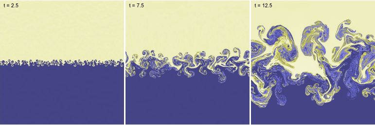
Kelvin-Helmholtz instability If we set the gravitational field to zero, $g=0$, we have the situation of a pure shear flow. In this case, the solutions of the dispersion relation are given by

$$\omega_{1/2}=\frac{k(\rho_{1}U_{1}+\rho_{2}U_{2})}{\rho_{1}+\rho_{2}}\pm ik\frac{\sqrt{\rho_{1}\rho_{2}}}{\rho_{1}+\rho_{2}}|U_{1}-U_{2}|.$$ (218)

Interestingly, in an ideal gas there is an imaginary growing mode component for every $|U_{1}-U_{2}|>0$! This means that a small wave-like perturbation at an interface will grow rapidly into large waves that take the form of characteristic Kelvin-Helmholtz “billows”. In the non-linear regime reached during the subsequent evolution of this instability the waves are rolled up, leading to the creation of vortex like structures, as seen in Figure 18. As the instability grows fastest for small scales (high $k$), the billows tend to get larger and larger with time.

7.2cm!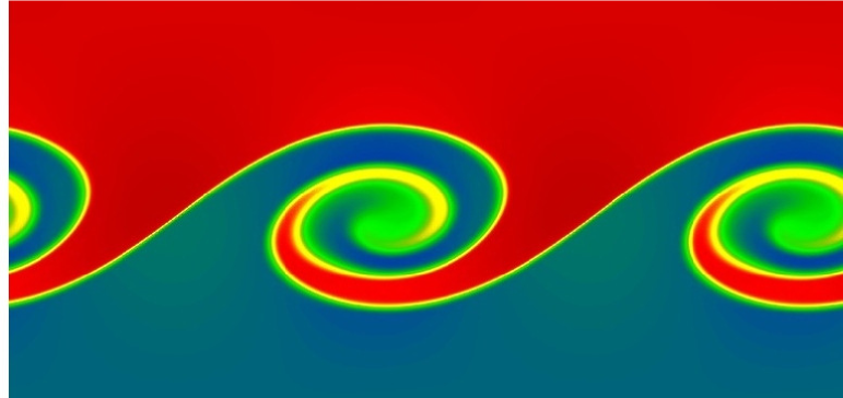

Figure 18: Characteristic Kelvin-Helmholtz billows arising in a shear flow.

Because the Kelvin-Helmholtz instability basically means that any sharp velocity gradient in a shear flow is unstable in a freely streaming fluid, this instability is particularly important for the creation of fluid turbulence. Under certain conditions, some modes can however be stabilized against the instability. This happens for example if we consider shearing with $U_{1}\neq U_{2}$ in a gravitational field $g>0$. Then the dispersion relation has the solutions

$$\omega=\frac{k(\rho_{1}U_{1}+\rho_{2}U_{2})}{\rho_{1}+\rho_{2}}\pm\frac{\sqrt{-k^{2}\rho_{1}\rho_{2}(U_{1}-U_{2})^{2}-(\rho_{1}+\rho_{2})(\rho_{2}-\rho_{1})kg}}{\rho_{1}+\rho_{2}}.$$ (219)

Stability is possible if two conditions are met. First, we need $\rho_{1}>\rho_{2}$, i.e. the lighter fluid needs to be on top (otherwise we would have in any case a Rayleigh-Taylor instability). Second, the condition

$$(U_{1}-U_{2})^{2}<\frac{(\rho_{1}+\rho_{2})(\rho_{1}-\rho_{2})g}{k\rho_{1}\rho_{2}}$$ (220)

must be fulfilled. Compared to the ordinary Kelvin-Holmholtz instability without a gravitational field, we hence see that sufficiently small wavelengths are stabilized below a threshold wavelength. The larger the shear becomes, the further this threshold moves to small scales.

The Rayleigh-Taylor and Kelvin-Helmholtz instabilities are by no means the only fluid instabilities that can occur in an ideal gas (Pringle & King, 2007). For example, there is also the Richtmyer-Meshov instability, which can occur when an interface is suddenly accelerated, for example due to the passage of a shock wave. In self-gravitating gases, there is the Jeans instability, which occurs when the internal gas pressure is not strong enough to prevent a positive density perturbation from growing and collapsing under its own gravitational attraction. This type of instability is particularly important in cosmic structure growth and star formation. If the gas dynamics is coupled to external sources of heat (e.g. through a radiation field), a number of further instabilities are possible. For example, a thermal instability (Field, 1965) can occur when a radiative cooling function has a negative dependence on temperature. If the temperature drops somewhere a bit more through cooling than elsewhere, the cooling rate of this cooler patch will increase such that it is cooling even faster. In this way, cool clouds can drop out of the background gas.

5.4 Turbulence

Fluid flow which is unsteady, irregular, seemingly random, and chaotic is called turbulent (Pope, 2000). Familiar examples of such situations include the smoke from a chimney, a waterfall, or the wind field behind a fast car or airplane. The characteristic feature of turbulence is that the fluid velocity varies significantly and irregularly both in position and time. As a result, turbulence is a statistical phenomenon and is best described with statistical techniques.

If the turbulent motions are subsonic, the flow can often be approximately treated as being incompressible, even for an equation of state that is not particularly stiff. Then only solenoidal motions that are divergence free can occur, or in other words, only shear flows are present. We have already seen that such flows are subject to fluid instabilities such as the Kelvin-Helmholtz instability, which can easily produce swirling motions on many different scales. Such vortex-like motions, also called eddies, are the conceptual building blocks of Kolmogorov’s theory of incompressible turbulence (Kolmogorov, 1941), which yields a surprisingly accurate description of the basic phenomenology of turbulence, even though many aspects of turbulence are still not fully understood.

Kolmogorov’s theory of incompressible turbulence

We consider a fully turbulent flow with characteristic velocity $U_{0}$ and length scale $L_{0}$. We assume that a quasi-stationary state for the turbulence is achieved by some kind of driving process on large scales, which in a time-averaged way injects an energy $\epsilon$ per unit mass. We shall also assume that the Reynolds number ${\rm Re}$ is large. We further imagine that the turbulent flow can be considered to be composed of eddies of different size $l$, with characteristic velocity $u(l)$, and associated timescale $\tau(l)=l/u(l)$.

For the largest eddies, $l\sim L_{0}$ and $u(l)\sim U_{0}$, hence viscosity is unimportant for them. But large eddies are unstable und break up, transferring their energy to somewhat smaller eddies. This continues to yet smaller scales, until

$${\rm Re}(l)=\frac{lu(l)}{\nu}$$ (221)

reaches of order unity, where $\nu$ is the kineamtic viscosity. For these eddies, viscosity will be very important so that their kinetic energy is dissipated away. We will see that this transfer of energy to smaller scales gives rise to the energy cascade of turbulence. But several important questions are still unanswered:

1. What is the actual size of the smallest eddies that dissipate the energy?

2. How do the velocities $u(l)$ of the eddies vary with $l$ when the eddies become smaller?

Kolmogorov’s hypotheses Kolmogorov conjectured a number of hypotheses that can answer these questions. In particular, he proposed:

• For high Reynolds number, the small-scale turbulent motions ($l\ll L_{0}$) become statistically isotropic. Any memory of large-scale boundary conditions and the original creation of the turbulence on large scales is lost.

• For high Reynolds number, the statistics of small-scale turbulent motions has a universal form and is only determined by $\nu$ and the energy injection rate per unit mass, $\epsilon$.

From $\nu$ and $\epsilon$, one can construct characteristic Kolmogorov length, velocity and timescales. Of particular importance is the Kolmogorov length:

$$\eta\equiv\left(\frac{\nu^{3}}{\epsilon}\right)^{1/4}.$$ (222)

Velocity and timescales are given by

$$u_{\eta}=(\epsilon\nu)^{1/4},\;\;\;\;\;\;\;\tau_{\eta}=\left(\frac{\nu}{\epsilon}\right)^{1/2}.$$ (223)

We then see that the Reynolds number at the Kolmogorov scales is

$${\rm Re}(\eta)=\frac{\eta u_{\eta}}{\nu}=1,$$ (224)

showing that they describe the dissipation range. Kolmogorov has furthermore made a second similarity hypothesis, as follows:

• For high Reynolds number, there is a range of scales $L_{0}\gg l\gg\eta$ over which the statistics of the motions on scale $l$ take a universal form, and this form is only determined by $\epsilon$, independent of $\nu$.

In other words, this also means that viscous effects are unimportant over this range of scales, which is called the inertial range. Given an eddy size $l$ in the inertial range, one can construct its characteristic velocity and timescale just from $l$ and $\epsilon$:

$$u(l)=(\epsilon l)^{1/3},\hskip 28.45274pt\tau(l)=\left(\frac{l^{2}}{\epsilon}\right)^{1/3}.$$ (225)

One further consequence of the existence of the inertial range is that here the energy transfer rate

$$T(l)\sim\frac{u^{2}(l)}{\tau(l)}$$ (226)

of eddies to smaller scales is expected to be scale-invariant. Indeed, putting in the expected characteristic scale dependence we get $T(l)\sim\epsilon$, i.e. $T(l)$ is equal to the energy injection rate. This also implies that we have

$$\epsilon\sim\frac{U_{0}^{3}}{L_{0}}.$$ (227)

With this result we can also work out what we expect for the ratio between the characteristic quantities of the largest and smallest scales:

$$\frac{\eta}{L_{0}}\sim\left(\frac{\nu^{3}}{\epsilon L_{0}^{4}}\right)^{1/4}=\left(\frac{\nu^{3}}{U_{0}^{3}L_{0}^{3}}\right)^{1/4}={\rm Re}^{-\frac{3}{4}},$$ (228)

$$\frac{u_{\eta}}{U_{0}}\sim\left(\frac{\epsilon\nu}{U_{0}^{4}}\right)^{1/4}=\left(\frac{U_{0}^{3}\nu}{L_{0}U_{0}^{4}}\right)^{1/4}={\rm Re}^{-\frac{1}{4}},$$ (229)

$$\frac{\tau_{\eta}}{\tau}\sim\left(\frac{\nu U_{0}^{2}}{\epsilon L_{0}^{2}}\right)^{1/2}=\left(\frac{\nu U_{0}^{2}L_{0}}{U_{0}^{3}L_{0}^{2}}\right)^{1/2}={\rm Re}^{-\frac{1}{2}}.$$ (230)

This shows that the Reynolds number directly sets the dynamic range of the inertial range.

Energy spectrum of Kolmogorov turbulence

Eddy motions on a length-scale $l$ correspond to wavenumber $k=2\pi/l$. The kinetic energy $\Delta E$ contained between two wave numbers $k_{1}$ and $k_{2}$ can be described by

$$\Delta E=\int_{k_{1}}^{k_{2}}E(k)\,{\rm d}k,$$ (231)

where $E(k)$ is the so-called energy spectrum. For the inertial range in Kolmogorov’s theory, we know that $E(k)$ is a universal function that only depends on $\epsilon$ and $k$. Hence $E(k)$ must be of the form

$$E(k)=C\,\epsilon^{a}\,k^{b},$$ (232)

where $C$ is a dimensionless constant. Through dimensional analysis it is easy to see that one must have $a=2/3$ and $b=-5/3$. We hence obtain the famous $-5/3$ slope of the Kolmogorov energy power spectrum:

$$E(k)=C\,\epsilon^{2/3}\,k^{-5/3}.$$ (233)

The constant $C$ is universal in Kolmogorov’s theory, but cannot be computed from first principles. Experiment and numerical simulations give $C\simeq 1.5$ (Pope, 2000).

7.3cm!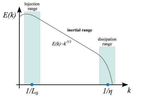

Figure 19: Schematic energy spectrum of Kolmogorov turbulence.

Actually, if we recall Kolmogorov’s first similarity hypothesis, it makes the stronger claim that the statistics for all small scale motion is universal. This means that also the dissipation part of the turbulence must have a universal form. To include this in the description of the spectrum, we can for example write

$$E(k)=C\,\epsilon^{2/3}\,k^{-5/3}f_{\eta}(k\eta),$$ (234)

where $f_{\eta}(k\eta)$ us a universal function with $f_{\eta}(x)=1$ for $x\ll 1$, and with $f_{\eta}(x)\to 0$ for $x\to\infty$. This function has to be determined experimentally or numerically. A good fit to different results is given by

$$f_{\eta}(x)=\exp\left(-\beta[(x^{4}+c^{4})^{1/4}-c]\right),$$ (235)

with $\beta_{0}\sim 5.2$ and $c\sim 0.4$ (Pope, 2000).

6 Eulerian hydrodynamics

Many physical theories are expressed as partial differential equations (PDEs), including some of the most fundamental laws of nature, such as fluid dynamics (Euler and Navier Stokes equations), electromagnetism (Maxwell’s equations) or general relativity/gravity (Einstein’s field equations). Broadly speaking, partial differential equations (PDE) are equations describing relations between partial derivatives of a dependent variable with respect to several independent variables. Unlike for ordinary differential equations (ODEs), there is no simple unified theory for PDEs. Rather, there are different types of PDEs which exhibit special features (Renardy & Rogers, 2004).

The Euler equations, which will be the focus of this section, are so-called hyperbolic conservation laws. They are non-linear, because they contain non-linear terms in the unknown functions and/or its partial derivatives. We note that a full characterization of the different types of PDEs goes beyond the scope of these lecture notes.

6.1 Solution schemes for PDEs

Unfortunately, for partial differential equations one cannot give a general solution method that works equally well for all types of problems. Rather, each type requires different approaches, and certain PDEs encountered in practice may even be best addressed with special custom techniques built by combining different elements from standard techniques. Important classes of solution schemes include the following:

• Finite difference methods: Here the differential operators are approximated through finite difference approximations, usually on a regular (cartesian) mesh, or some other kind of structured mesh (for example a polar grid). An example we already previously discussed is Poisson’s equation treated with iterative (multigrid) methods.

• Finite volume methods: These may be seen as a subclass of finite difference methods. They are particularly useful for hyperbolic conservation laws. We shall discuss examples for this approach in applications to fluid dynamics later in this section.

• Spectral methods: Here the solution is represented by a linear combination of functions, allowing the PDE to be transformed to algebraic equations or ordinary differential equations. Often this is done by applying Fourier techniques. For example, solving the Poisson equation with FFTs, as we discussed earlier, is a spectral method.

• Method of lines: This is a semi-discrete approach where all derivatives except for one are approximated with finite differences. The remaining derivative is then the only one left, so that the remaining problem forms a set of ordinary differential equations (ODEs). Very often, this approach is used in time-dependent problems. One here discretizes space in terms of a set of $N$ points ${x_{i}}$, and for each of these points one obtains an ODE that describes the time evolution of the function at this point. The PDE is transformed in this way into a set of $N$ coupled ODEs. For example, consider the heat diffusion equation in one dimension,

  $$\frac{\partial u}{\partial t}+\lambda\frac{\partial^{2}u}{\partial x^{2}}=0.$$ (236)

  If we discretize this into a set of points that are spaced $h$ apart, we obtain $N$ equations

  $$\frac{{\rm d}u_{i}}{{\rm d}t}+\lambda\frac{u_{i+1}+u_{i-1}-2u_{i}}{h^{2}}=0.$$ (237)

  These differential equations can now be integrated in time as an ODE system. Note however that this is not necessarily stable. Some problems may require upwinding, i.e. asymmetric forms for the finite difference estimates to recover stability.

• Finite element methods: Here the domain is subdivided into “cells” (elements) of fairly arbitrary shape. The solution is then represented in terms of simple, usually polynomial functions on the element, and then the PDE is transformed to an algebraic problem for the coefficients in front of these simple functions. This is hence similar in spirit to spectral methods, except that the expansion is done in terms of highly localized functions on an element by element basis, and is truncated already at low order.

In practice, many different variants of these basic methods exist, and sometimes also combinations of them are used.

6.2 Simple advection

First-order equations of hyperbolic type are particularly useful for introducing the numerical difficulties that then also need to be addressed for more complicated non-linear conservation laws (e.g. Toro, 1997; LeVeque, 2002; Stone et al., 2008). The simplest equation of this type is the advection equation in one dimension. This is given by

$$\frac{\partial u}{\partial t}+v\cdot\frac{\partial u}{\partial x}=0,$$ (238)

where $u=u(x,t)$ is a function of $x$ and $t$, and $v$ is a constant parameter. This equation is hyperbolic because the so-called coefficient matrix is real and trivially diagonalizable.

If we are given any function $q(x)$, then

$$u(x,t)=q(x-vt)$$ (240)

is a solution of the PDE, as one can easily check. We can interpret $u(x,t=0)=q(x)$ as initial condition, and the solution at a later time is then an exact copy of $q$, simply translated by $v\,t$ along the $x$-direction, as shown in Fig. 20.

Figure 20: Simple advection with constant velocity to the right.

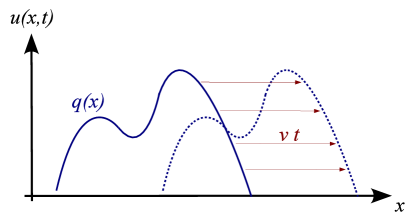
Points that start at a certain coordinate $x_{0}$ are advected to a new location $x_{\rm ch}(t)=vt+x_{0}$. These so-called characteristics (see Fig. 21), which can be viewed as mediating the propagation of information in the system, are straight lines, all oriented in the downstream direction. Note that “downstream” refers to the direction in which the flow goes, whereas “upstream” is from where the flow comes.

7.3cm!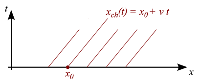

Figure 21: A set of flow characteristics for advection to the right with constant velocity $v$.

Let’s now assume we want to solve the advection problem numerically. (Strictly speaking this is of course superfluous as we have an analytic solution in this case, but we want to see how well a numerical technique would perform here.) We can approach this with a straightforward discretization of $u$ on a special mesh, using for example the method of lines. This gives us:

$$\frac{{\rm d}u_{i}}{{\rm d}t}+v\frac{u_{i+1}-u_{i-1}}{2h}=0.$$ (241)

If we go one step further and also discretize the time derivative with a simple Euler scheme, we get

$$u_{i}^{(n+1)}=u_{i}^{(n)}-v\frac{u_{i+1}^{(n)}-u_{i-1}^{(n)}}{2h}\Delta t.$$ (242)

This is a complete update formula which can be readily applied to a given initial state on the grid. The big surprise is that this turns out to be quite violently unstable! For example, if one applies this to the advection of a step function, one invariably obtains strong oscillatory errors in the downstream region of the step, quickly rendering the numerical solution into complete garbage. What is the reason for this fundamental failure?

• First note that all characteristics (signals) propagate downstream in this problem, or in other words, information strictly travels in the flow direction in this problem.

• But, the information to update $u_{i}$ is derived both from the upstream ($u_{i-1}$) and the downstream ($u_{i+1}$) side.

• According to how the information flows, $u_{i}$ should not really depend on the downstream side at all, which in some sense is causally disconnected. So let’s try to get rid off this dependence by going to a one-sided approximation for the spatial derivative, of the form:

  $$\frac{{\rm d}u_{i}}{{\rm d}t}+v\frac{u_{i}-u_{i-1}}{h}=0.$$ (243)

  This is called upwind differencing. Interestingly, now the stability problems are completely gone!

• But there are still some caveats to observe: First of all, the discretization now depends on the sign of $v$. For negative $v$, one instead has to use

  $$\frac{{\rm d}u_{i}}{{\rm d}t}+v\frac{u_{i+1}-u_{i}}{h}=0.$$ (244)

  The other is that the solution is not advected in a perfectly faithful way, instead it is quite significantly smoothed out, through a process one calls numerical diffusion.

We can actually understand where this strong diffusion in the 1st-order upwind scheme comes from. To this end, let’s rewrite the upwind finite difference approximation of the spatial derivative as

$$\frac{u_{i}-u_{i-1}}{h}=\frac{u_{i+1}-u_{i-1}}{2h}-\frac{u_{i+1}-2u_{i}+u_{i-1}}{2h}.$$ (245)

Hence our stable upwind scheme can also be written as

$$\frac{{\rm d}u_{i}}{{\rm d}t}+v\frac{u_{i+1}-u_{i-1}}{2h}=\frac{vh}{2}\,\frac{u_{i+1}-2u_{i}+u_{i-1}}{h^{2}}.$$ (246)

But recall from equation (133) that

$$\left(\frac{\partial^{2}u}{\partial x^{2}}\right)_{i}\simeq\frac{u_{i+1}-2u_{i}+u_{i-1}}{h^{2}},$$ (247)

so if we define a diffusion constant $D=(vh)/2$, we are effectively solving the following problem,

$$\frac{\partial u}{\partial t}+v\cdot\frac{\partial u}{\partial x}=D\frac{\partial^{2}u}{\partial x^{2}},$$ (248)

and not the original advection problem. The diffusion term on the right hand side is here a byproduct of the numerical algorithm that we have used. We needed to add this numerical diffusion in order to obtain stability of the integration.

Note however that for better grid resolution, $h\to 0$, the diffusion becomes smaller, so in this limit one obtains an ever better solution. Also note that the diffusivity becomes larger for larger velocity $v$, so the faster one needs to advect, the stronger the numerical diffusion effects become.

Besides the upwinding requirement, integrating a hyperbolic conservation law with an explicit method in time also requires the use of a sufficiently small integration timestep, not only to get sufficiently good accuracy, but also for reasons of stability. In essence, there is a maximum timestep that may be used before the integration brakes down. How large can we make this timestep? Again, we can think about this in terms of information travel. If the timestep exceeds $\Delta t_{\rm max}=h/v$, then the updating of $u_{i}$ would have to include information from $u_{i-2}$, but if we don’t do this, the updating will likely become unstable.

This leads to the so-called Courant-Friedrichs-Levy (CFL) timestep condition (Courant et al., 1928), which for this problem takes the form

$$\Delta t\leq\frac{h}{v}.$$ (249)

This is a necessary but not sufficient condition for any explicit finite different approach of the hyperbolic advection equation. For other hyperbolic conservation laws, similar CFL-conditions apply.

Hyperbolic conservation laws We now consider a hyperbolic conservation law, such as the continuity equation for the mass density of a fluid:

$$\frac{\partial\rho}{\partial t}+\nabla\cdot(\rho\vec{v})=0.$$ (250)

We see that this is effectively the advection equation, but with a spatially variable velocity $\vec{v}=\vec{v}(\vec{x})$. Here $\vec{F}=\rho\vec{v}$ is the mass flux.

6.8cm!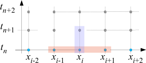

Figure 22: A discretization scheme for the continuity equation in one spatial dimension. The red and blue boxes mark the stencils that are applied for calculating the spatial and time derivatives.

Let’s study the problem in one spatial dimension, and consider a discretization both of the $x$- and $t$-axis. This corresponds to

$$\frac{\rho_{i}^{(n+1)}-\rho_{i}^{(n)}}{\Delta t}+\frac{F_{i+1}^{(n)}-F_{i-1}^{(n)}}{2\Delta x}=0,$$ (251)

leading to the update rule

$$\rho_{i}^{(n+1)}=\rho_{i}^{(n)}+\frac{\Delta t}{2\Delta x}\left(F_{i-1}^{(n)}-F_{i+1}^{(n)}\right).$$ (252)

This is again found to be highly unstable, for the same reasons as in the plain advection problem: we have not observed in ‘which direction the wind blows’, or in other words, we have ignored in which direction the local characteristics point. For example, if the mass flux is to the right, we know that the characteristics point also to the right. The upwind direction is therefore towards negative $x$, and by using only this information in making our spatial derivative one-sided, we should be able to resurrect stability.

Now, for the mass continuity equation identifying the local characteristics is quite easy, and in fact, their direction can simply be inferred from the sign of the mass flux. However, in more general situations for systems of non-linear PDEs, this is far less obvious. Here we need to use a so-called Riemann solvers to give us information about the local solution and the local characteristics (Toro, 1997). This then also implicitly identifies the proper upwinding that is needed for stability.

6.3 Riemann problem

The Riemann problem is an initial value problem for a hyperbolic system, consisting of two piece-wise constant states (two half-spaces) that meet at a plane at $t=0$. The task is then to solve for the subsequent evolution at $t>0$.

An important special case is the Riemann problem for the Euler equations (i.e. for ideal gas dynamics). Here the left and right states of the interface, can, for example, be uniquely specified by giving the three “primitive” variables density, pressure and velocity, viz.

$$U_{L}=\left(\begin{array}[]{c}\rho_{L}\\ P_{L}\\ \vec{v}_{L}\end{array}\right),\;\;\;\;U_{R}=\left(\begin{array}[]{c}\rho_{R}\\ P_{R}\\ \vec{v}_{R}\end{array}\right).$$ (253)

Alternatively one can also specify density, momentum density, and energy density. For an ideal gas, this initial value problem can be solved analytically (Toro, 1997), modulo an implicit equation which requires numerical root-finding, i.e. the solution cannot be written down explicitly. The solution always contains characteristics for three self-similar waves, as shown schematically in Fig. 23. Some notes on this:

7.5cm!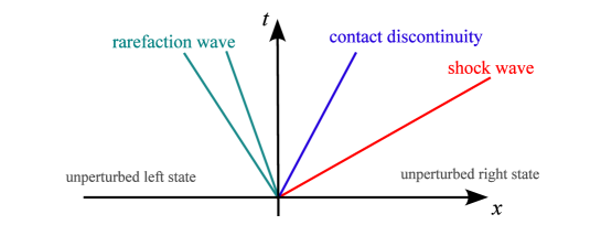

Figure 23: Wave structure of the solution of the Riemann problem. The central contact wave separates the original fluid phases. On the left and the right, there is either a shock or a rarefaction wave.

• The middle wave is always present and is a contact wave that marks the boundary between the original fluid phases from the left and right sides.

• The contact wave is sandwiched between a shock or a rarefaction wave on either side (it is possible to have shocks on both sides, or rarefactions on both sides, or one of each). The rarefaction wave is not a single characteristic but rather a rarefaction fan with a beginning and an end.

• These waves propagate with constant speed. If the solution is known at some time $t>0$, it can also be obtained at any other time through a suitable scaling transformation. An important corollary is that at $x=0$, the fluid quantities $(\rho^{\star},P^{\star},\vec{v}^{\star})$ are constant in time for $t>0$.

• For $\vec{v}_{L}=\vec{v}_{R}=0$, the Riemann problem simplifies and becomes the ‘Sod shock tube’ problem.

Figure 24: Initial state of an example Riemann problem, composed of two phases in different states that are brought into contact at $x=0$ at time $t=0$. (Since $v_{x}=0$, the initial conditions are actually an example of the special case of a Sod shock-tube problem.)

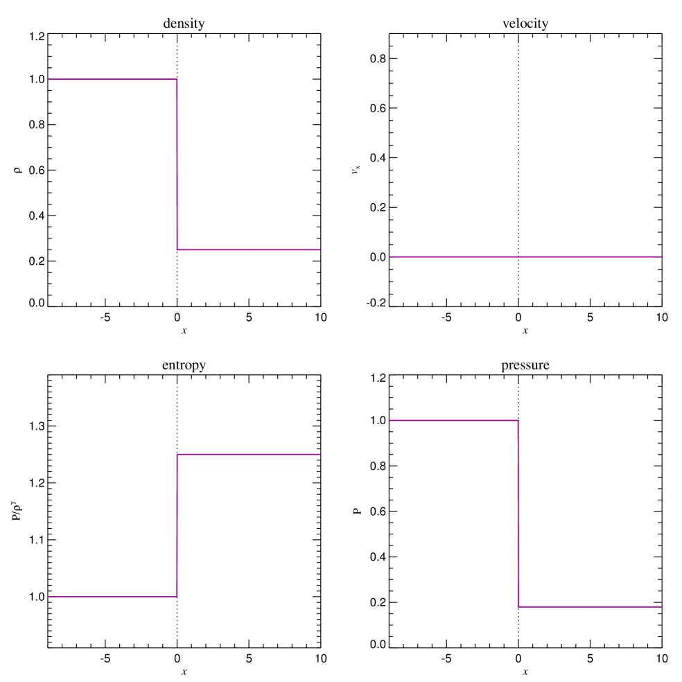
Let’s consider an example how this wave structure looks in a real Riemann problem. We consider, for definiteness, a Riemann problem with $\rho_{L}=1.0$, $P_{L}=1.0$, $v_{L}=0$, and $\rho_{R}=0.25$, $P_{R}=0.1795$, $v_{R}=0$ (which is of Sod-shock type). The adiabatic exponent is taken to be $\gamma=1.4$. We hence deal at $t=0.0$ with the initial state displayed in Figure 24. After time $t=5.0$, the wave structure formed by a rarefaction to the left (location marked in green), a contact in the middle (blue) and a shock to the right (red) can be nicely seen in Figure 25.

Figure 25: Evolved state at $t=5.0$ of the initial fluid state displayed in Fig. 24. The blue dashed line marks the position of the contact wave, the green dashed lines give the location of the rarefaction fan, and the red dashed line marks the shock.

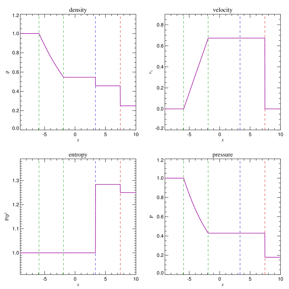
Some general properties of the waves appearing in the Riemann problem can be summarized as follows:

• Shock: This is a sudden compression of the fluid, associated with an irreversible conversion of kinetic energy to heat, i.e. here entropy is produced. The density, normal velocity component, pressure, and entropy all change discontinuously at a shock.

• Contact discontinuity: This traces the original separating plane between the two fluid phases that have been brought into contact. Pressure as well as the normal velocity are constant across a contact, but density, entropy and temperature can jump.

• Rarefaction wave: This occurs when the gas (suddenly) expands. The rarefaction wave smoothly connects two states over a finite spatial region; there are no discontinuities in any of the fluid variables.

6.4 Finite volume discretization

Let’s now take a look how Riemann solvers can be used in the finite volume discretization approach to the PDEs of fluid dynamics. Recall that we can write our hyperbolic conservation laws as

$$\frac{\partial\vec{U}}{\partial t}+\nabla\cdot\vec{F}=0.$$ (254)

Here $\vec{U}$ is a state vector and $\vec{F}$ is the flux vector. For example, the Euler equations of section 5.1 can be written in the form

$$\vec{U}=\left(\begin{array}[]{c}\rho\\ \rho\vec{v}\\ \rho e\end{array}\right),\;\;\;\;\;\;\;\vec{F}=\left(\begin{array}[]{c}\rho\vec{v}\\ \rho\vec{v}\vec{v}^{T}+P\\ (\rho e+P)\vec{v}\end{array}\right),$$ (255)

with the specific energy $e=u+\vec{v}^{2}/2$ and $u$ being the thermal energy per unit mass. The ideal gas equation gives the pressure as $P=(\gamma-1)\rho u$ and provides a closure for the system.

In a finite volume scheme, we describe the system through the averaged state over a set of finite cells. These cell averages are defined as

$$\vec{U}_{i}=\frac{1}{V_{i}}\int_{{\rm cell}\;i}\vec{U}(\vec{x})\,{\rm d}V.$$ (256)

Let’s now see how we could divise an update scheme for these cell-averaged quantities.

1. We start by integrating the conservation law over a cell, and over a finite interval in time:

   $$\int_{x_{i-\frac{1}{2}}}^{x_{i+\frac{1}{2}}}{\rm d}x\int_{t_{n}}^{t_{n+1}}{\rm d}t\left(\frac{\partial\vec{U}}{\partial t}+\frac{\partial\vec{F}}{\partial x}\right)=0.$$ (257)

2. This gives

   $$\int_{x_{i-\frac{1}{2}}}^{x_{i+\frac{1}{2}}}{\rm d}x\left[\vec{U}(x,t_{n+1})-\vec{U}(x,t_{n})\right]+\int_{t_{n}}^{t_{n+1}}{\rm d}t\left[\vec{F}(x_{i+\frac{1}{2}},t)-\vec{F}(x_{i-\frac{1}{2}},t)\right]=0.$$ (258)

   In the first term, we recognize the definition of the cell average:

   $$\vec{U}_{i}^{(n)}\equiv\frac{1}{\Delta x}\int_{x_{i-\frac{1}{2}}}^{x_{i+\frac{1}{2}}}\vec{U}(x,t_{n}){\rm d}x.$$ (259)

   Hence we have

   $$\Delta x\left[\vec{U}_{i}^{(n+1)}-\vec{U}_{i}^{(n)}\right]+\int_{t_{n}}^{t_{n+1}}{\rm d}t\left[\vec{F}(x_{i+\frac{1}{2}},t)-\vec{F}(x_{i-\frac{1}{2}},t)\right]=0.$$ (260)

3. Now, $\vec{F}(x_{i+\frac{1}{2}},t)$ for $t>t_{n}$ is given by the solution of the Riemann problem with left state $\vec{U}_{i}^{(n)}$ and right state $\vec{U}_{i+1}^{(n)}$. At the interface, this solution is independent of time. We can hence write

   $$\vec{F}(x_{i+\frac{1}{2}},t)=\vec{F}^{\star}_{i+\frac{1}{2}},$$ (261)

   where $\vec{F}^{\star}_{i+\frac{1}{2}}=\vec{F}_{\rm Riemann}(\vec{U}_{i}^{(n)},\vec{U}_{i+1}^{(n)})$ is a short-hand notation for the corresponding Riemann solution sampled at the interface. Hence we now get

   $$\Delta x\left[\vec{U}_{i}^{(n+1)}-\vec{U}_{i}^{(n)}\right]+\Delta t\left[\vec{F}^{\star}_{i+\frac{1}{2}}-\vec{F}^{\star}_{i-\frac{1}{2}}\right]=0.$$ (262)

   Or alternative, as an explicit update formula:

   $$\vec{U}_{i}^{(n+1)}=\vec{U}_{i}^{(n)}+\frac{\Delta t}{\Delta x}\left[\vec{F}^{\star}_{i-\frac{1}{2}}-\vec{F}^{\star}_{i+\frac{1}{2}}\right].$$ (263)

   The first term in the square bracket gives the flux that flows from left into the cell, the second term is the flux out of the cell on its right side. The idea to use the Riemann solution in the updating step is due to Godunov, that’s why such schemes are often called Godunov schemes.

It is worthwhile to note that we haven’t really made any approximation in the above (yet). In particular, if we calculate $\vec{F}_{\rm Riemann}$ analytically (and hence exactly), then the above seems to account for the correct fluxes for arbitrarily long times. So does this mean that we get a perfectly accurate result even for very large timesteps? This certainly sounds too good to be true, so there must be a catch somewhere.

Indeed, there is. First of all, we have assumed that the Riemann problems are independent of each other and each describe infinite half-spaces. This is not true once we consider finite volume cells, but it is still ok for a while as long $t_{n+1}$ is close enough to $t_{n}$ such that the waves emanating in one interface have not yet arrived at the next interface left or right. This then leads to a CFL-timestep criterion, were $\Delta t\leq\Delta x/c_{\rm max}$ and $c_{\rm max}$ is the maximum wavespeed.

Another point is more subtle and comes into play when we consider more than one timestep. We assumed that the $\vec{U}_{i}^{(n)}$ describe piece-wise constant states which can then be fed to the Riemann solver to give us the flux. However, even when this is true initially, we have just seen that after one timestep it will not be true anymore. By ignoring this in the subsequent timestep (which is done by performing an averaging step that washes out the cell substructure that developed as part of the evolution during the previous timestep) we make some error.

6.5 Godunov’s method and Riemann solvers

It is useful to introduce another interpretation of common finite-volume discretizations of fluid dynamics, so-called Reconstruct-Evolve-Average (REA) schemes. We also use this here for a short summary of Godunov’s important method, and the way Riemann solvers come into play in it.

7.4cm!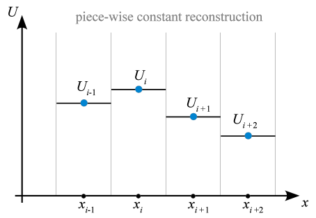

Figure 26: Piece-wise constant states of a fluid forming the simplest possible reconstruction of its state based on a set of discrete values $U_{i}$ known at spatial positions $x_{i}$.

An REA update scheme of a hydrodynamical system discretized on a mesh can be viewed as a sequence of three steps:

1. Reconstruct: Using the cell-averaged quantities (as shown in Fig. 26), this defines the run of these quantities everywhere in the cell. In the sketch, a piece-wise constant reconstruction is assumed, which is the simplest procedure one can use and leads to 1st order accuracy.

2. Evolve: The reconstructed state is then evolved forward in time by $\Delta t$. In Godunov’s approach, this is done by treating each cell interface as a piece-wise constant initial value problem which is solved with the Riemann solver exactly or approximately. This solution is formally valid as long as the waves emanating from opposite sides of a cell do not yet start to interact. In practice, one therefore needs to limit the timestep $\Delta t$ such that this does not happen.

3. Average: The wave structure resulting from the evolution over timestep $\Delta t$ is spatially averaged in a conservative fashion to compute new states $\vec{U}^{n+1}$ for each cell. Fortunately, the averaging step does not need to be done explicitly; instead it can simply be carried out by accounting for the fluxes that enter or leave the control volume of the cell. Then the whole cycle repeats again.

What is needed for the evolve step is a prescription to either exactly or approximately solve the Riemann problem for a piece-wise linear left and right state that are brought into contact at time $t=t_{n}$. Formally, this can be written as

$$\vec{F}^{\star}=\vec{F}_{\rm Riemann}(\vec{U}_{L},\vec{U}_{R}).$$ (264)

In practice, a variety of approximate Riemann solvers $\vec{F}_{\rm Riemann}$ are commonly used in the literature (Rusanov, 1961; Harten et al., 1983; Toro, 1997; Miyoshi & Kusano, 2005). For the ideal gas and for isothermal gas, it is also possible to solve the Riemann problem exactly, but not in closed form (i.e. the solution involves an iterative root finding of a non-linear equation).

There are now two main issues left:

• How can this be extended to multiple spatial dimensions?

• How can it be extended such that a higher order integration accuracy both in space and time is reached?

We’ll discuss these issues next.

6.6 Extensions to multiple dimensions

So far, we have considered one-dimensional hyperbolic conservation laws of the form

$$\partial_{t}\vec{U}+\partial_{x}\vec{F(U)}=0,$$ (265)

where $\partial_{t}$ is a short-hand notation for $\partial_{t}=\frac{\partial}{\partial t}$, and similarly $\partial_{x}=\frac{\partial}{\partial x}$. For example, for isothermal gas with soundspeed $c_{s}$, the state vector $\vec{U}$ and flux vector $\vec{F}(\vec{U})$ are given as

$$\vec{U}=\left(\begin{array}[]{c}\rho\\ \rho u\\ \end{array}\right),\;\;\;\vec{F}=\left(\begin{array}[]{c}\rho u\\ \rho u^{2}+\rho c_{s}^{2}\\ \end{array}\right),$$ (266)

where $u$ is the velocity in the $x$-direction.

In three dimensions, the PDEs describing a fluid become considerably more involved. For example, the Euler equations for an ideal gas are given in explicit form as

$$\partial_{t}\left(\begin{array}[]{c}\rho\\ \rho u\\ \rho v\\ \rho w\\ \rho e\\ \end{array}\right)+\partial_{x}\left(\begin{array}[]{c}\rho u\\ \rho u^{2}+P\\ \rho uv\\ \rho uw\\ \rho u(\rho e+P)\\ \end{array}\right)+\partial_{y}\left(\begin{array}[]{c}\rho v\\ \rho uv\\ \rho v^{2}+P\\ \rho vw\\ \rho v(\rho e+P)\\ \end{array}\right)+\partial_{z}\left(\begin{array}[]{c}\rho w\\ \rho uw\\ \rho vw\\ \rho w^{2}+P\\ \rho w(\rho e+P)\\ \end{array}\right)=0,$$ (267)

where $e=e_{\rm therm}+(u^{2}+v^{2}+w^{2})/2$ is the total specific energy per unit mass, $e_{\rm therm}$ is the thermal energy per unit mass, and $P=(\gamma-1)\rho\,e_{\rm therm}$ is the pressure. These equations are often written in the following notation:

$$\partial_{t}\vec{U}+\partial_{x}\vec{F}+\partial_{y}\vec{G}+\partial_{z}\vec{H}=0.$$ (268)

Here the functions $\vec{F(U)}$, $\vec{G(U)}$ and $\vec{H(U)}$ give the flux vectors in the $x$-, $y$- and $z$-direction, respectively.

Dimensional splitting

Let us now consider the three dimensionally split problems derived from equation (268):

$$\partial_{t}\vec{U}+\partial_{x}\vec{F}=0,$$ (269)

$$\partial_{t}\vec{U}+\partial_{y}\vec{G}=0,$$ (270)

$$\partial_{t}\vec{U}+\partial_{z}\vec{H}=0.$$ (271)

Note that the vectors appearing here have still the same dimensionality as in the full equations. They are augmented one-dimensional problems, i.e. the transverse variables still appear but spatial differentiation happens only in one direction. Because of this, these additional transverse variables do not make the 1D problem more difficult compared to the ‘pure’ 1D problem considered earlier, but the fluxes appearing in them still need to be included.

Now let us assume that he have a method to solve/advance each of these one-dimensional problems. We can for example express this formally through time-evolution operators ${\cal X}(\Delta t$), ${\cal Y}(\Delta t)$, and ${\cal Z}(\Delta t)$, which advance the solution by a timestep $\Delta t$. Then the full time advance of the system can for example be approximated by

$$\vec{U}^{n+1}\simeq{\cal Z}(\Delta t){\cal Y}(\Delta t){\cal X}(\Delta t)\vec{U}^{n}.$$ (272)

This is one possible dimensionally split update scheme. In fact, this is the exact solution if equations (269)-(270) represent the linear advection problem, but for more general non-linear equations it only provides a first order approximation. However, higher-order dimensionally split update schemes can also be easily constructed. For example, in two-dimensions,

$$\vec{U}^{n+1}=\frac{1}{2}[{\cal X}(\Delta t){\cal Y}(\Delta t)+{\cal Y}(\Delta t){\cal X}(\Delta t)]\vec{U}^{n}$$ (273)

and

$$\vec{U}^{n+1}={\cal X}(\Delta t/2){\cal Y}(\Delta t){\cal X}(\Delta t/2)\vec{U}^{n}$$ (274)

are second-order accurate. Similarly, for three dimensions the scheme

$$\vec{U}^{n+1}={\cal X}(\Delta t/2){\cal Y}(\Delta t/2){\cal Z}(\Delta t){\cal Y}(\Delta t/2){\cal X}(\Delta t/2)\vec{U}^{n}$$ (275)

is second-order accurate. As a general rule of thumb, the time evolution operators have to be applied alternatingly in reverse order to reach second-order accuracy. We see that the dimensionless splitting reduces the problem effectively to a sequence of one-dimensional solution operations which are applied to multi-dimensional domains. Note that each one-dimensional operator leads to an update of $\vec{U}$, and is a complete step for the corresponding augmented one-dimensional problem. Gradients, etc., that are needed for the next step then have to be recomputed before the next time-evolution operator is applied. In practical applications of mesh codes, these one-dimensional solves are often called sweeps.

Unsplit schemes

Figure 27: Sketch of unsplit finite-volume update schemes. On the left, the case of a structured Cartesian grid is shown, the case on the right is for an unstructured grid.

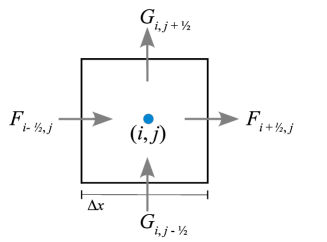
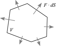
In an unsplit approach, all flux updates of a cell are applied simultaneously to a cell, not sequentially. This is for example illustrated in 2D in the situations depicted in Figure 27. The unsplit update of cell $i,j$ in the Cartesian case is then given by

$$U_{i,j}^{n+1}=U_{i,j}^{n}+\frac{\Delta t}{\Delta x}\left(\vec{F}_{i-\frac{1}{2},j}-\vec{F}_{i+\frac{1}{2},j}\right)+\frac{\Delta t}{\Delta y}\left(\vec{G}_{i,j-\frac{1}{2}}-\vec{G}_{i,j+\frac{1}{2}}\right).$$ (276)

Unsplit approaches can also be used for irregular shaped cells like those appearing in unstructured meshes (see Fig. 27). For example, integrating over a cell of volume $V$ and denoting with $\vec{U}$ the cell average, we can write the cell update with the divergence theorem as

$$\vec{U}^{n+1}=\vec{U}^{n}-\frac{\Delta t}{V}\int\vec{F}\,\cdot\vec{dS},$$ (277)

where the integration is over the whole cell surface, with outwards pointing face area vectors $\vec{dS}$.

6.7 Extensions for high-order accuracy

We should first clarify what we mean with higher order schemes. Loosely speaking, this refers to the convergence rate of a scheme in smooth regions of a flow. For example, if we know the analytic solution $\rho(x)$ for some problem, and then obtain a numerical result $\rho_{i}$ at a set of $N$ points at locations $x_{i}$, we can ask what the typical error of the solution is. One possibility to quantify this would be through a L1 error norm, for example in the form

$$L1=\frac{1}{N}\sum_{i}|\rho_{i}-\rho(x_{i})|,$$ (278)

which can be interpreted as the average error per cell. If we now measure this error quantitatively for different resolutions of the applied discretization, we would like to find that L1 decreases with increasing $N$. In such a case our numerical scheme is converging, and provided we use sufficient numerical resources, we have a chance to get below any desired absolute error level. But the rate of convergence can be very different between different numerical schemes when applied to the same problem. If a method shows a $L1\propto N^{-1}$ scaling, it is said to be first-order accurate; a doubling of the number of cells will then cut the error in half. A second-order method has $L1\propto N^{-2}$, meaning that a doubling of the number of cells can actually reduce the error by a factor of 4. This much better convergence rate is of course highly desirable. It is also possible to construct schemes with still higher convergence rates, but they tend to quickly become much more complex and computationally involved, so that one eventually reaches a point of diminishing return, depending on the specific type of problem. But the extra effort one needs to make to go from first to second-order is often very small, sometimes trivially small, so that one basically should always strive to try at least this.

6.5cm!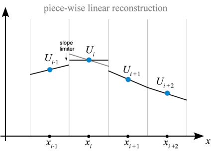

Figure 28: Piece-wise linear reconstruction scheme applied to a fluid state represented through a regular mesh.

A first step in constructing a 2nd order extension of Godunov’s method is to replace the piece-wise constant with a piece-wise linear reconstruction. This requires that one first estimates gradients for each cell (usually by a simple finite difference formula). These are then slope-limited if needed such that the linear extrapolations of the cell states to the cell interfaces do not introduce new extrema. This slope-limiting procedure is quite important; it needs to be done to avoid that real fluid discontinuities introduce large spurious oscillations into the fluid.

Given slope limited gradients, for example $\nabla\rho$ for the density, one can then estimate the left and right states adjacent to an interface $x_{i+\frac{1}{2}}$ by spatial extrapolation from the centers of the cells left and right from the interface:

$$\rho_{i+\frac{1}{2}}^{L} = \rho_{i}+(\nabla\rho)_{i}\,\frac{\Delta x}{2},$$ (279)

$$\rho_{i+\frac{1}{2}}^{R} = \rho_{i+1}-(\nabla\rho)_{i+1}\,\frac{\Delta x}{2}.$$ (280)

The next step would in principle be to use these states in the Riemann solver. In doing this we will ignore the fact that our reconstruction has now a gradient over the cell; instead we still pretend that the fluid state can be taken as piece-wise constant left and right of the interface as far as the Riemann solver is concerned. However, it turns out that the spatial extrapolation needs to be augmented with a temporal extrapolation one half timestep into the future, such that the flux estimate is now effectively done in the middle of the timestep. This is necessary both to reach second-order accuracy in time and also for stability reasons. Hence we really need to use

$$\rho_{i+\frac{1}{2}}^{L} = \rho_{i}+(\nabla\rho)_{i}\,\frac{\Delta x}{2}+\left(\frac{\partial\rho}{\partial t}\right)_{i}\,\frac{\Delta t}{2},$$ (281)

$$\rho_{i+\frac{1}{2}}^{R} = \rho_{i+1}-(\nabla\rho)_{i+1}\,\frac{\Delta x}{2}+\left(\frac{\partial\rho}{\partial t}\right)_{i+1}\,\frac{\Delta t}{2},$$ (282)

for extrapolating to the interfaces. More generally, this has to be done for the whole state vector of the system, i.e.

$$\vec{U}_{i+\frac{1}{2}}^{L} = \vec{U}_{i}+(\partial_{x}\vec{U})_{i}\,\frac{\Delta x}{2}+(\partial_{t}\vec{U})_{i}\,\frac{\Delta t}{2},$$ (283)

$$\vec{U}_{i+\frac{1}{2}}^{R} = \vec{U}_{i+1}-(\partial_{x}\vec{U})_{i+1}\,\frac{\Delta x}{2}+(\partial_{t}\vec{U})_{i+1}\,\frac{\Delta t}{2}.$$ (284)

Note that here the quantity $(\partial_{x}\vec{U})_{i}$ is a (slope-limited) estimate of the gradient in cell $i$, based on finite-differences plus a slope limiting procedure. Similarly, we somehow need to estimate the time derivative encoded in $(\partial_{x}\vec{U})_{i}$. How can this be done? One way to do this is to exploit the Jacobian matrix of the Euler equations. We can write the Euler equations as

$$\partial_{t}\vec{U}=-\partial_{x}\vec{F}(\vec{U})=-\frac{\partial\vec{F}}{\partial\vec{U}}\,\partial_{x}\vec{U}=-\vec{A}(\vec{U})\,\partial_{x}\vec{U},$$ (285)

where $\vec{A(U)}$ is the Jacobian matrix. Using this, we can simply estimate the required time-derivative based on the spatial derivatives:

$$(\partial_{t}\vec{U})_{i}=-\vec{A}(\vec{U}_{i})\,(\partial_{x}\vec{U})_{i}.$$ (286)

Hence the extrapolation can be done as

$$\vec{U}_{i+\frac{1}{2}}^{L} = \vec{U}_{i}+\left[\frac{\Delta x}{2}-\frac{\Delta t}{2}\vec{A}(\vec{U}_{i})\right](\partial_{x}\vec{U})_{i},$$ (287)

$$\vec{U}_{i+\frac{1}{2}}^{R} = \vec{U}_{i+1}+\left[-\frac{\Delta x}{2}-\frac{\Delta t}{2}\vec{A}(\vec{U}_{i+1})\right](\partial_{x}\vec{U})_{i+1}.$$ (288)

This procedure defines the so-called MUSCL-Hancock scheme (van Leer, 1984; Toro, 1997; van Leer, 2006), which is a 2nd-order accurate extension of Godunov’s method.

Higher-order extensions such as the piece-wise parabolic method (PPM) start out with a higher order polynomial reconstruction. In the case of PPM, parabolic shapes are assumed in each cell instead of piece-wise linear states. The reconstruction is still guaranteed to be conservative, i.e. the integral underneath the reconstruction recovers the total values of the conserved variables individually in each cell. So-called ENO and WENO schemes (e.g. Balsara et al., 2009) use yet higher-order polynomials to reconstruct the state in a conservative fashion. Here many more cells in the environment need to be considered (i.e. the so-called stencil of these methods is much larger) to robustly determine the coefficients of the reconstruction. This can for example involve a least-square fitting procedure (Ollivier-Gooch, 1997).

7 Smoothed particle hydrodynamics

Smoothed Particle Hydrodynamics (SPH) is a technique for approximating the continuum dynamics of fluids through the use of particles, which may also be viewed as interpolation points (SPH; Lucy, 1977; Gingold & Monaghan, 1977; Monaghan, 1992; Springel, 2010b). The principal idea of SPH is to treat hydrodynamics in a completely mesh-free fashion, in terms of a set of sampling particles. Hydrodynamical equations of motion are then derived for these particles, yielding a quite simple and intuitive formulation of gas dynamics. Moreover, it turns out that the particle representation of SPH has excellent conservation properties. Energy, linear momentum, angular momentum, mass, and entropy (if no artificial viscosity operates) are all simultaneously conserved. In addition, there are no advection errors in SPH, and the scheme is fully Galilean invariant, unlike alternative mesh-based Eulerian techniques. Due to its Lagrangian character, the local resolution of SPH follows the mass flow automatically, a property that is convenient in representing the large density contrasts often encountered in astrophysical problems.

7.1 Kernel interpolation

At the heart of smoothed particle hydrodynamics lie so-called kernel interpolants. In particular, we use a kernel summation interpolant for estimating the density, which then determines the rest of the basic SPH equations through the variational formalism.

For any field $F(\vec{r})$, we may define a smoothed interpolated version, $F_{s}(\vec{r})$, through a convolution with a kernel $W(\vec{r},h)$:

$$F_{s}(\vec{r})=\int F(\vec{r}^{\prime})\,W(\vec{r}-\vec{r}^{\prime},h)\,{\rm d}\vec{r}^{\prime}.$$ (289)

Here $h$ describes the characteristic width of the kernel, which is normalized to unity and approximates a Dirac $\delta$-function in the limit $h\to 0$. We further require that the kernel is symmetric and sufficiently smooth to make it at least differentiable twice. One possibility for $W$ is a Gaussian. However, most current SPH implementations are based on kernels with a finite support. Usually a cubic spline is adopted with $W(r,h)=w(\frac{r}{2h})$, and

$$w_{\rm 3D}(q)=\frac{8}{\pi}\left\{\begin{array}[]{ll}1-6q^{2}+6q^{3},&0\leq q\leq\frac{1}{2},\\ 2\left(1-q\right)^{3},&\frac{1}{2}<q\leq 1,\\ 0,&q>1,\end{array}\right.$$ (290)

in three-dimensional normalization, but recent work also considered various alternative kernels (Read et al., 2010; Dehnen & Aly, 2012). Through Taylor expansion, it is easy to see that the above kernel interpolant is second-order accurate for regularly distributed points due to the symmetry of the kernel.

Figure 29: Kernel interpolation with a B-spline kernel.

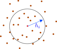
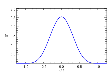
Suppose now we know the field at a set of points $\vec{r}_{i}$, i.e. $F_{i}=F(\vec{r}_{i})$. The points have an associated mass $m_{i}$ and density $\rho_{i}$, such that $V_{i}\sim m_{i}/\rho_{i}$ is their associated finite volume element. Provided the points sufficiently densely sample the kernel volume, we can approximate the integral in Eqn. (289) with the sum

$$F_{s}(\vec{r})\simeq\sum_{j}\frac{m_{j}}{\rho_{j}}\,F_{j}\,W(\vec{r}-\vec{r}_{j},h).$$ (291)

This is effectively a Monte-Carlo integration, except that thanks to the comparatively regular distribution of points encountered in practice, the accuracy is better than for a random distribution of the sampling points. In particular, for points in one dimension with equal spacing $d$, one can show that for $h=d$ the sum of Eqn. (291) provides a second order accurate approximation to the real underlying function. Unfortunately, for the irregular yet somewhat ordered particle configurations encountered in real applications, a formal error analysis is not straightforward. It is clear however, that at the very least one should have $h\geq d$, which translates to a minimum of $\sim 33$ neighbors in 3D if a Cartesian point distribution is assumed.

Importantly, we see that the estimate for $F_{s}(\vec{r})$ is defined everywhere (not only at the underlying points), and is differentiable thanks to the differentiability of the kernel, albeit with a considerably higher interpolation error for the derivative. Moreover, if we set $F(\vec{r})=\rho(\vec{r})$, we obtain

$$\rho_{s}(\vec{r})\simeq\sum_{j}m_{j}W(\vec{r}-\vec{r}_{j},h),$$ (292)

yielding a density estimate just based on the particle coordinates and their masses. In general, the smoothing length can be made variable in space, $h=h(\vec{r},t)$, to account for variations in the sampling density. This adaptivity is one of the key advantages of SPH and is essentially always used in practice. There are two options to introduce the variability of $h$ into Eqn. (292). One is by adopting $W(\vec{r}-\vec{r}_{j},h(\vec{r}))$ as kernel, which corresponds to the so-called ‘scatter’ approach (Hernquist & Katz, 1989). It has the advantage that the volume integral of the smoothed field recovers the total mass, $\int\rho_{s}(\vec{r})\,{\rm d}\vec{r}=\sum_{i}m_{i}$. On the other hand, the so-called ‘gather’ approach, where we use $W(\vec{r}-\vec{r}_{j},h(\vec{r}_{i}))$ as kernel in Eqn. (292), requires only knowledge of the smoothing length $h_{i}=h(\vec{r}_{i})$ for estimating the density of particle $i$, which leads to computationally convenient expressions when the variation of the smoothing length is consistently included in the SPH equations of motion. Since the density is only needed at the coordinates of the particles and the total mass is conserved anyway (since it is tied to the particles), it is not important that the volume integral of the gather form of $\rho_{s}(\vec{r})$ exactly equals the total mass.

In the following we drop the subscript $s$ for indicating the smoothed field, and adopt as SPH estimate of the density of particle $i$ the expression

$$\rho_{i}=\sum_{j=1}^{N}m_{j}\,W(\vec{r}_{i}-\vec{r}_{j},h_{i}).$$ (293)

It is clear now why kernels with a finite support are preferred. They allow the summation to be restricted to the $N_{\rm ngb}$ neighbors that lie within the spherical region of radius $2h$ around the target point $\vec{r}_{i}$, corresponding to a computational cost of order ${\cal O}(N_{\rm ngb}\,N)$ for the full density estimate. Normally this number $N_{\rm ngb}$ of neighbors within the support of the kernel is approximately (or exactly) kept constant by choosing the $h_{i}$ appropriately. $N_{\rm ngb}$ hence represents an important parameter of the SPH method and needs to be made large enough to provide sufficient sampling of the kernel volumes. Kernels like the Gaussian on the other hand would require a summation over all particles $N$ for every target particle, resulting in a ${\cal O}(N^{2})$ scaling of the computational cost.

If SPH was really a Monte-Carlo method, the accuracy expected from the interpolation errors of the density estimate would be rather problematic. But the errors are much smaller because the particles do not sample the fluid in a Poissonian fashion. Instead, their distances tend to equilibrate due to the pressure forces, which makes the interpolation errors much smaller (Price, 2012). Yet, they remain a significant source of error in SPH and are ultimately the primary origin of the noise inherent in SPH results (Bauer & Springel, 2012).

Even though we have based most of the above discussion on the density, the general kernel interpolation technique can also be applied to other fields, and to the construction of differential operators. For example, we may write down a smoothed velocity field and take its derivative to estimate the local velocity divergence, yielding:

$$(\nabla\cdot\vec{v})_{i}=\sum_{j}\frac{m_{j}}{\rho_{j}}\vec{v}_{j}\cdot\nabla_{i}W(\vec{r}_{i}-\vec{r}_{j},h).$$ (294)

However, an alternative estimate can be obtained by considering the identity $\rho\nabla\cdot\vec{v}=\nabla(\rho\vec{v})-\vec{v}\cdot\nabla\rho$, and computing kernel estimates for the two terms on the right hand side independently. Their difference then yields

$$(\nabla\cdot\vec{v})_{i}=\frac{1}{\rho_{i}}\sum_{j}m_{j}(\vec{v}_{j}-\vec{v}_{i})\cdot\nabla_{i}W(\vec{r}_{i}-\vec{r}_{j},h).$$ (295)

This pair-wise formulation turns out to be more accurate in practice. In particular, it has the advantage of always providing a vanishing velocity divergence if all particle velocities are equal.

7.2 SPH equations of motion

The Euler equations for inviscid gas dynamics in Lagrangian form are given by

$$\frac{{\rm d}\rho}{{\rm d}t}+\rho\,\nabla\cdot\vec{v}=0,$$ (296)

$$\frac{{\rm d}\vec{v}}{{\rm d}t}+\frac{\nabla P}{\rho}=0,$$ (297)

$$\frac{{\rm d}u}{{\rm d}t}+\frac{P}{\rho}\nabla\cdot\vec{v}=0,$$ (298)

where ${\rm d}/{\rm d}t=\partial/\partial t+\vec{v}\cdot\nabla$ is the convective derivative. This system of partial differential equations expresses conservation of mass, momentum and energy. Eckart (1960) has shown that the Euler equations for an inviscid ideal gas follow from the Lagrangian

$$L=\int\rho\left(\frac{\vec{v}^{2}}{2}-u\right)\,{\rm d}V.$$ (299)

This opens up an interesting route for obtaining discretized equations of motion for gas dynamics. Instead of working with the continuum equations directly and trying to heuristically work out a set of accurate difference formulas, one can discretize the Lagrangian and then derive SPH equations of motion by applying the variational principals of classical mechanics (Springel & Hernquist, 2002). Using a Lagrangian also immediately guarantees certain conservation laws and retains the geometric structure imposed by Hamiltonian dynamics on phase space.

We start by discretizing the Lagrangian in terms of fluid particles of mass $m_{i}$, yielding

$$L_{\rm SPH}=\sum_{i}\left(\frac{1}{2}m_{i}{\vec{v}_{i}^{2}}-m_{i}u_{i}\right),$$ (300)

where it has been assumed that the thermal energy per unit mass of a particle can be expressed through an entropic function $A_{i}$ of the particle, which simply labels its specific thermodynamic entropy. The pressure of the particles is

$$P_{i}=A_{i}\rho_{i}^{\gamma}=(\gamma-1)\rho_{i}u_{i},$$ (301)

where $\gamma$ is the adiabatic index. Note that for isentropic flow (i.e. in the absence of shocks, and without mixing or thermal conduction) we expect the $A_{i}$ to be constant. We hence define $u_{i}$, the thermal energy per unit mass, in terms of the density estimate as

$$u_{i}(\rho_{i})=A_{i}\frac{\rho_{i}^{\gamma-1}}{\gamma-1}.$$ (302)

This raises the question of how the smoothing lengths $h_{i}$ needed for estimating $\rho_{i}$ should be determined. As we discussed above, we would like to ensure adaptive kernel sizes, meaning that the number of points in the kernel should be approximately constant. In much of the older SPH literature, the number of neighbors was allowed to vary within some (small) range around a target number. Sometimes the smoothing length itself was evolved with a differential equation in time, exploiting the continuity relation and the expectation that $\rho h^{3}$ should be approximately constant. In case the number of neighbors outside the kernel happened to fall outside the allowed range, $h$ was suitably readjusted, at the price of some errors in energy conservation.

A better method is to require that the mass in the kernel volume should be constant, viz.

$$\rho_{i}h_{i}^{3}=const$$ (303)

for three dimensions. Since $\rho_{i}=\rho_{i}(\vec{r}_{1},\vec{r}_{2},\ldots\vec{r}_{N},h_{i})$ is only a function of the particle coordinates and of $h_{i}$, this equation implicitly defines the function $h_{i}=h_{i}(\vec{r}_{1},\vec{r}_{2},\ldots\vec{r}_{N})$ in terms of the particle coordinates.

We can then proceed to derive the equations of motion from

$$\frac{{\rm d}}{{\rm d}t}\frac{\partial L}{\partial\dot{\vec{r}}_{i}}-\frac{\partial L}{\partial\vec{r}_{i}}=0.$$ (304)

This first gives

$$m_{i}\frac{{\rm d}\vec{v}_{i}}{{\rm d}t}=-\sum_{j=1}^{N}m_{j}\frac{P_{j}}{\rho_{j}^{2}}\,\frac{\partial\rho_{j}}{\partial\vec{r}_{i}},$$ (305)

where the derivative $\partial\rho_{j}/\partial\vec{r}_{i}$ stands for the total variation of the density with respect to the coordinate $\vec{r}_{i}$, including any variation of $h_{j}$ this may entail. We can hence write

$$\frac{\partial\rho_{j}}{\partial\vec{r}_{i}}=\vec{\nabla}_{i}\rho_{j}+\frac{\partial\rho_{j}}{\partial h_{j}}\frac{\partial h_{j}}{\partial\vec{r}_{i}},$$ (306)

where the smoothing length is kept constant in the first derivative on the right hand side (in our notation, the Nabla operator $\nabla_{i}=\partial/\partial\vec{r}_{i}$ means differentiation with respect to $\vec{r}_{i}$ holding the smoothing lengths constant). On the other hand, differentiation of $\rho_{j}h_{j}^{3}=const$ with respect to $\vec{r}_{i}$ yields

$$\frac{\partial\rho_{j}}{\partial h_{j}}\frac{\partial h_{j}}{\partial\vec{r}_{i}}\left[1+\frac{3\,\rho_{j}}{h_{j}}\left(\frac{\partial\rho_{j}}{\partial h_{j}}\right)^{-1}\right]=-\vec{\nabla}_{i}\rho_{j}.$$ (307)

Combining equations (306) and (307) we then find

$$\frac{\partial\rho_{j}}{\partial\vec{r}_{i}}=\left(1+\frac{h_{j}}{3\rho_{j}}\frac{\partial\rho_{j}}{\partial h_{j}}\right)^{-1}\vec{\nabla}_{i}\rho_{j}.$$ (308)

Using

$$\nabla_{i}{\rho_{j}}=m_{i}\nabla_{i}W_{ij}(h_{j})+\delta_{ij}\sum_{k=1}^{N}m_{k}\nabla_{i}W_{ki}(h_{i})\,,$$ (309)

we finally obtain the equations of motion

$$\frac{{\rm d}\vec{v}_{i}}{{\rm d}t}=-\sum_{j=1}^{N}m_{j}\left[f_{i}\frac{P_{i}}{\rho_{i}^{2}}\nabla_{i}W_{ij}(h_{i})+f_{j}\frac{P_{j}}{\rho_{j}^{2}}\nabla_{i}W_{ij}(h_{j})\right],$$ (310)

where the $f_{i}$ are defined by

$$f_{i}=\left[1+\frac{h_{i}}{3\rho_{i}}\frac{\partial\rho_{i}}{\partial h_{i}}\right]^{-1},$$ (311)

and the abbreviation $W_{ij}(h)=W(|\vec{r}_{i}-\vec{r}_{j}|,h)$ has been used. Note that the correction factors $f_{i}$ can be easily calculated alongside the density estimate, all that is required is an additional summation to get $\partial\rho_{i}/\partial\vec{r}_{i}$ for each particle. This quantity is in fact also useful to get the correct smoothing radii by iteratively solving $\rho_{i}h_{i}^{3}=const$ with a Newton-Raphson iteration (Springel & Hernquist, 2002).

The equations of motion (310) for inviscid hydrodynamics are remarkably simple. In essence, we have transformed a complicated system of partial differential equations into a much simpler set of ordinary differential equations. Furthermore, we only have to solve the momentum equation explicitly. The mass conservation equation as well as the total energy equation (and hence the thermal energy equation) are already taken care of, because the particle masses and their specific entropies stay constant for reversible gas dynamics. However, later we will introduce an artificial viscosity that is needed to allow a treatment of shocks. This will introduce additional terms in the equation of motion and requires the time integration of one thermodynamic quantity per particle, which can either be chosen as entropy or thermal energy. Indeed, the above formulation can also be equivalently expressed in terms of thermal energy instead of entropy. This follows by taking the time derivative of Eqn. (302), which first yields

$$\frac{{\rm d}u_{i}}{{\rm d}t}=\frac{P_{i}}{\rho_{i}^{2}}\sum_{j}\vec{v}_{j}\cdot\frac{\partial\rho_{i}}{\partial\vec{r}_{j}}.$$ (312)

Using equations (308) and (309) then gives the evolution of the thermal energy as

$$\frac{{\rm d}u_{i}}{{\rm d}t}=f_{i}\frac{P_{i}}{\rho_{i}^{2}}\sum_{j}m_{j}(\vec{v}_{i}-\vec{v}_{j})\cdot\vec{\nabla}W_{ij}(h_{i}),$$ (313)

which needs to be integrated along the equation of motion if one wants to use the thermal energy as independent thermodynamic variable. There is no difference however to using the entropy; the two are completely equivalent in the variational formulation.

Note that the above formulation readily fulfills the conservation laws of energy, momentum and angular momentum. This can be shown based on the discretized form of the equations, but it is also manifest due to the symmetries of the Lagrangian that was used as a starting point. The absence of an explicit time dependence gives the energy conservation, the translational invariance implies momentum conservation, and the rotational invariance gives angular momentum conservation.

7.3 Artificial Viscosity

Even when starting from perfectly smooth initial conditions, the gas dynamics described by the Euler equations may readily produce true discontinuities in the form of shock waves and contact discontinuities. At such fronts the differential form of the Euler equations breaks down, and their integral form (equivalent to the conservation laws) needs to be used. At a shock front, this yields the Rankine-Hugoniot jump conditions that relate the upstream and downstream states of the fluid. These relations show that the specific entropy of the gas always increases at a shock front, implying that in the shock layer itself the gas dynamics can no longer be described as inviscid. In turn, this also implies that the discretized SPH equations we derived above can not correctly describe a shock, simply because they keep the entropy strictly constant.

One thus must allow for a modification of the dynamics at shocks and somehow introduce the necessary dissipation. This is usually accomplished in SPH by an artificial viscosity. Its purpose is to dissipate kinetic energy into heat and to produce entropy in the process. The usual approach is to parameterize the artificial viscosity in terms of a friction force that damps the relative motion of particles. Through the viscosity, the shock is broadened into a resolvable layer, something that makes a description of the dynamics everywhere in terms of the differential form possible. It may seem a daunting task though to somehow tune the strength of the artificial viscosity such that just the right amount of entropy is generated in a shock. Fortunately, this is however relatively unproblematic. Provided the viscosity is introduced into the dynamics in a conservative fashion, the conservation laws themselves ensure that the right amount of dissipation occurs at a shock front.

What is more problematic is to devise the viscosity such that it is only active when there is really a shock present. If it also operates outside of shocks, even if only at a weak level, the dynamics may begin to deviate from that of an ideal gas.

The viscous force is most often added to the equation of motion as

$$\left.\frac{{\rm d}\vec{v}_{i}}{{\rm d}t}\right|_{\rm visc}=-\sum_{j=1}^{N}m_{j}\Pi_{ij}\nabla_{i}\overline{W}_{ij}\,,$$ (314)

where

$$\overline{W}_{ij}=\frac{1}{2}\left[W_{ij}(h_{i})+W_{ij}(h_{j})\right]$$ (315)

denotes a symmetrized kernel, which some researchers prefer to define as $\overline{W}_{ij}=W_{ij}([h_{i}+h_{j}]/2)$. Provided the viscosity factor $\Pi_{ij}$ is symmetric in $i$ and $j$, the viscous force between any pair of interacting particles will be antisymmetric and along the line joining the particles. Hence linear momentum and angular momentum are still preserved. In order to conserve total energy, we need to compensate the work done against the viscous force in the thermal reservoir, described either in terms of entropy,

$$\left.\frac{{\rm d}A_{i}}{{\rm d}t}\right|_{\rm visc}=\frac{1}{2}\frac{\gamma-1}{\rho_{i}^{\gamma-1}}\sum_{j=1}^{N}m_{j}\Pi_{ij}\vec{v}_{ij}\cdot\nabla_{i}\overline{W}_{ij}\,,$$ (316)

or in terms of thermal energy per unit mass,

$$\left.\frac{{\rm d}u_{i}}{{\rm d}t}\right|_{\rm visc}=\frac{1}{2}\sum_{j=1}^{N}m_{j}\Pi_{ij}\vec{v}_{ij}\cdot\nabla_{i}\overline{W}_{ij}\,,$$ (317)

where $\vec{v}_{ij}=\vec{v}_{i}-\vec{v}_{j}$. There is substantial freedom in the detailed parametrization of the viscosity $\Pi_{ij}$. The most commonly used formulation of the viscosity is

$$\Pi_{ij}=\left\{\begin{tabular}[]{cl}${\left[-\alpha c_{ij}\mu_{ij}+\beta\mu_{ij}^{2}\right]}/{\rho_{ij}}$&\mbox{if $\vec{v}_{ij}\cdot\vec{r}_{ij}<0$}\\ 0&\mbox{otherwise},\\ \end{tabular}\right.$$ (318)

with

$$\mu_{ij}=\frac{h_{ij}\,\vec{v}_{ij}\cdot\vec{r}_{ij}}{\left|\vec{r}_{ij}\right|^{2}+\epsilon h_{ij}^{2}}.$$ (319)

Here $h_{ij}$ and $\rho_{ij}$ denote arithmetic means of the corresponding quantities for the two particles $i$ and $j$, with $c_{ij}$ giving the mean sound speed, and $\vec{r}_{ij}\equiv\vec{r}_{i}-\vec{r}_{j}$. The strength of the viscosity is regulated by the parameters $\alpha$ and $\beta$, with typical values in the range $\alpha\simeq 0.5-1.0$ and the frequent choice of $\beta=2\,\alpha$. The parameter $\epsilon\simeq 0.01$ is introduced to protect against singularities if two particles happen to get very close.

In this form, the artificial viscosity is basically a combination of a bulk and a von Neumann-Richtmyer viscosity. Historically, the quadratic term in $\mu_{ij}$ has been added to the original Monaghan-Gingold form to prevent particle penetration in high Mach number shocks. Note that the viscosity only acts for particles that rapidly approach each other, hence the entropy production is always positive definite.

7.4 New trends in SPH

Smoothed particle hydrodynamics is a remarkably versatile and simple approach for numerical fluid dynamics. The ease with which it can provide a large dynamic range in spatial resolution and density, as well as an automatically adaptive resolution, are unmatched in Eulerian methods. At the same time, SPH has excellent conservation properties, not only for energy and linear momentum, but also for angular momentum. The latter is not automatically guaranteed in Eulerian codes, even though it is usually fulfilled at an acceptable level for well-resolved flows. When coupled to self-gravity, SPH conserves the total energy exactly, which is again not manifestly true in most mesh-based approaches to hydrodynamics. Finally, SPH is Galilean-invariant and free of any errors from advection alone, which is another advantage compared to Eulerian mesh-based approaches.

Thanks to its completely mesh-free nature, SPH can easily deal with complicated geometric settings and large regions of space that are completely devoid of particles. Implementations of SPH in a numerical code tend to be comparatively simple and transparent. At the same time, the scheme is characterized by remarkable robustness. For example, negative densities or negative temperatures, sometimes a problem in mesh-based codes, can not occur in SPH by construction. Although shock waves are broadened in SPH, the properties of the post-shock flow are correct.

The main disadvantage of SPH is its limited accuracy in multi-dimensional flows (e.g. Agertz et al., 2007; Bauer & Springel, 2012). One source of noise originates in the approximation of local kernel interpolants through discrete sums over a small set of nearest neighbors. While in 1D the consequences of this noise tend to be reasonably benign, particle motion in multiple dimensions has a much higher degree of freedom. Here the mutually repulsive forces of pressurized neighboring particle pairs do not easily cancel in all dimensions simultaneously, especially not given the errors of the discretized kernel interpolants. As a result, some ‘jitter’ in the particle motions readily develops, giving rise to velocity noise up to a few percent of the local sound speed. This noise seriously messes up the accuracy that can be reached with the technique, especially for subsonic flow, and also leads to a slow convergence rate.

Another problem is the relatively high numerical viscosity of SPH. To reduce the numerical viscosity of SPH in regions away from shocks, several studies have recently advanced the idea of keeping the functional form of the artificial viscosity, but making the viscosity strength parameter $\alpha$ variable in time (Morris, 1997; Dolag et al., 2005; Rosswog, 2005). Adopting $\beta=2\alpha$, one may for example evolve the parameter $\alpha$ individually for each particle with an equation such as

$$\frac{{\rm d}\alpha_{i}}{{\rm d}t}=-\frac{\alpha_{i}-\alpha_{\rm max}}{\tau_{i}}+S_{i},$$ (320)

where $S_{i}$ is some source function meant to ramp up the viscosity rapidly if a shock is detected, while the first term lets the viscosity exponentially decay again to a prescribed minimum value $\alpha_{\rm min}$ on a timescale $\tau_{i}$. So far, mostly simple source functions like $S_{i}=\max[-(\nabla\cdot\vec{v})_{i},0]$ and timescales $\tau_{i}\simeq h_{i}/c_{i}$ have been explored and the viscosity $\alpha_{i}$ has often also been prevented from becoming higher than some prescribed maximum value $\alpha_{\rm max}$. It is clear that the success of such a variable $\alpha$ scheme depends critically on an appropriate source function. The form above can still not distinguish purely adiabatic compression from that in a shock, so is not completely free of creating unwanted viscosity. More advanced parameterizations that try to address this problem have therefore also been developed (Cullen & Dehnen, 2010).

Particularly problematic in SPH are also fluid instabilities across contact discontinuities, such as Kelvin-Helmholtz instabilities. These are usually found to be suppressed in their growth. Recent new formulations of SPH try to improve on this either through different kernel shapes combined with a much larger number of smoothing neighbors (e.g. Read & Hayfield, 2012), through artificial thermal conduction at contact discontinuities to reduce pressure force errors and spurious surface tension there (e.g. Price, 2008), or by alluding to a pressure-based formulation where the density is estimated only indirectly from a kernel-interpolated pressure field (Hopkins, 2013). These developments appear certainly promising. At the moment many new ideas for improved SPH formulations are still advanced, and new implementations are published regularly. While many problems of SPH have been addresses by these new schemes, so far they have not yet been able to cure the relatively large gradient errors in SPH, suggesting that the convergence rate of them is still lower than that of comparable mesh-based approaches (e.g. Hu et al., 2014).

8 Moving-mesh techniques

8.1 Differences between Eulerian and Lagrangian techniques

It has become clear over recent years that both Lagrangian SPH and Eulerian AMR techniques suffer from fundamental limitations that make them inaccurate in certain regimes. Indeed, these methods sometimes yield conflicting results even for basic calculations that only consider non-radiative hydrodynamics (e.g. Frenk et al., 1999; Agertz et al., 2007; Tasker et al., 2008; Mitchell et al., 2009). SPH codes have comparatively poor shock resolution, offer only low-order accuracy for the treatment of contact discontinuities, and suffer from subsonic velocity noise. Worse, they appear to suppress fluid instabilities under certain conditions, as a result of a spurious surface tension and inaccurate gradient estimates across density jumps. On the other hand, Eulerian codes are not free of fundamental problems either. They do not produce Galilean-invariant results, which can make their accuracy sensitive to the presence of bulk velocities (e.g. Wadsley et al., 2008; Tasker et al., 2008). Another concern lies in the preference of certain spatial directions in Eulerian hydrodynamics, which can make poorly resolved disk galaxies align with the coordinate planes (Dubois et al., 2014).

There is hence substantial motivation to search for new hydrodynamical methods that improve on these weaknesses of the SPH and AMR techniques. In particular, we would like to retain the accuracy of mesh-based hydrodynamical methods (for which decades of experience have been accumulated in computational fluid dynamics), while at the same time we would like to outfit them with the Galilean-invariance and geometric flexibility that is characteristic of SPH. The principal idea for achieving such a synthesis is to allow the mesh to move with the flow itself. This is in principle an obvious and old idea (Braun & Sambridge, 1995; Gnedin, 1995; Whitehurst, 1995; Mavriplis, 1997; Xu, 1997; Hassan et al., 1998; Pen, 1998; Trac & Pen, 2004), but one fraught with many practical difficulties. In particular, mesh tangling (manifested in ‘bow-tie’ cells and hourglass like mesh motions) is the traditional problem of such attempts to simulate multi-dimensional hydrodynamics in a Lagrangian fashion.

8.2 Voronoi tessellations

We here briefly describe a new formulation of continuum hydrodynamics based on an unstructured mesh that overcomes many of these problems (Springel, 2010a). The mesh is defined as the Voronoi tessellation of a set of discrete mesh-generating points, which are in principle allowed to move freely. For the given set of points, the Voronoi tessellation of space consists of non-overlapping cells around each of the sites such that each cell contains the region of space closer to it than to any of the other sites. Closely related to the Voronoi tessellation is the Delaunay tessellation, the topological dual of the Voronoi diagram. Both constructions can also be used for natural neighbor interpolation and geometric analysis of cosmic structures (e.g. van de Weygaert, 1994; Pelupessy et al., 2003; van de Weygaert & Schaap, 2009). In 2D, the Delaunay tessellation for a given set of points is a triangulation of the plane, where the points serve as vertices of the triangles. The defining property of the Delaunay triangulation is that each circumcircle around one of the triangles of the tessellation is not allowed to contain any of the other mesh-generating points in its interior. This empty circumcircle property distinguishes the Delaunay triangulation from the many other triangulations of the plane that are possible for the point set, and in fact uniquely determines the triangulation for points in general position. Similarly, in three dimensions, the Delaunay tessellation is formed by tetrahedra that are not allowed to contain any of the points inside their circumspheres.

7.5cm!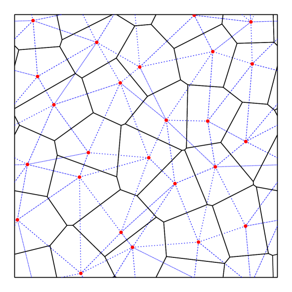

Figure 30: Example of a Voronoi and Delaunay tessellation in 2D, with periodic boundary conditions. The red circles show the generating points of the Voronoi tessellation, which is drawn with solid lines. Its topological dual, the Delaunay triangulation, is overlaid with thin dashed lines.

As an example, Figure 30 shows the Delaunay and Voronoi tessellations for a small set of points in 2D, enclosed in a box with imposed periodic boundary conditions. The midpoints of the circumcircles around each Delaunay triangle form the vertices of the Voronoi cells, and for each line in the Delaunay diagram, there is an orthogonal face in the Voronoi tessellation.

The Voronoi cells can be used as control volumes for a finite-volume formulation of hydrodynamics, using the same principal ideas for reconstruction, evolution and averaging (REA) steps that we have discussed earlier in the context of Eulerian techniques. However, as we will discuss below it is possible to consistently include the mesh motion in the formulation of the numerical steps, allowing the REA-scheme to become Galilean-invariant. Even more importantly, due to the mathematical properties of the Voronoi tessellation, the mesh continuously deforms and changes its topology as a result of the point motion, without ever leading to the dreaded mesh-tangling effects that are the curse of traditional moving mesh methods.

8.3 Finite volume hydrodynamics on a moving mesh

As already discussed earlier in section 6.4, the Euler equations are conservation laws for mass, momentum and energy that take the form of a system of hyperbolic partial differential equation. They can be written in the compact form

$$\frac{\partial\vec{U}}{\partial t}+\vec{\nabla}\cdot\vec{F}=0,$$ (321)

which emphasizes their character as conservation laws.

Following the finite-volume strategy, we describe the fluid’s state by the cell-averages of the conserved quantities for these cells. In particular, integrating the fluid over the volume $V_{i}$ of cell $i$, we can define the total mass $m_{i}$, momentum $p_{i}$ and energy $E_{i}$ contained in the cell as follows,

$$\vec{Q}_{i}=\left(\begin{array}[]{c}m_{i}\\ \vec{p}_{i}\\ E_{i}\end{array}\right)=\int_{V_{i}}\vec{U}\,{\rm d}V.$$ (322)

With the help of the Euler equations, we can calculate the rate of change of $\vec{Q}_{i}$ in time. Converting the volume integral over the flux divergence into a surface integral over the cell results in

$$\frac{{\rm d}\vec{Q}_{i}}{{\rm d}t}=-\int_{\partial V_{i}}\left[\vec{F}(\vec{U})-\vec{U}\vec{w}^{T}\right]{\rm d}\vec{n}.$$ (323)

Here $\vec{n}$ is an outward normal vector of the cell surface, and $\vec{w}$ is the velocity with which each point of the boundary of the cell moves. In Eulerian codes, the mesh is taken to be static, so that $\vec{w}=0$, while in a fully Lagrangian approach, the surface would move at every point with the local flow velocity, i.e. $\vec{w}=\vec{v}$. In this case, the right hand side of equation (323) formally simplifies, because then the first component of $\vec{Q}_{i}$, the mass, stays fixed for each cell. Unfortunately, it is normally not possible to follow the distortions of the shapes of fluid volumes exactly in multi-dimensional flows for a reasonably long time, or in other words, one cannot guarantee the condition $\vec{w}=\vec{v}$ over the entire surface. In this case, one needs to use the general formula of equation (323). As an aside, we note that one conceptual problem of SPH is that these surface fluxes due to the $\vec{w}$-term are always ignored.

The cells of our finite volume discretization are polyhedra with flat polygonal faces (or lines in 2D). Let $\vec{A}_{ij}$ describe the oriented area of the face between cells $i$ and $j$ (pointing from $i$ to $j$). Then we can define the averaged flux across the face $i$-$j$ as

$$\vec{{F}}_{ij}=\frac{1}{A_{ij}}\int_{A_{ij}}\left[\vec{F}(\vec{U})-\vec{U}\vec{w}^{T}\right]{\rm d}\vec{A}_{ij},$$ (324)

and the Euler equations in finite-volume form become

$$\frac{{\rm d}\vec{Q}_{i}}{{\rm d}t}=-\sum_{j}A_{ij}\vec{F}_{ij}.$$ (325)

We obtain a manifestly conservative time discretization of this equation by writing it as

$$\vec{Q}_{i}^{(n+1)}=\vec{Q}_{i}^{(n)}-\Delta t\sum_{j}A_{ij}\vec{{\hat{F}}}_{ij}^{(n+1/2)},$$ (326)

where the $\vec{{\hat{F}}}_{ij}$ are now an appropriately time-averaged approximation to the true flux $\vec{F}_{ij}$ across the cell face. The notation $\vec{Q}_{i}^{(n)}$ is meant to describe the state of the system at step $n$. Note that $\vec{{\hat{F}}}_{ij}$ = $-\vec{{\hat{F}}}_{ji}$, i.e. the discretization is manifestly conservative.

Figure 31: Sketch of a Voronoi mesh and the relevant geometric quantities that enter the flux calculation across a face. In (a), we show the the mesh-generating points $\vec{r}_{i}$ and $\vec{r}_{j}$ of two cells $i$ and $j$. The face between these two cells has a center-of-mass vector $\vec{f}_{ij}$, which in general will be offset from the mid-point $m_{ij}$ of the two points. In (b), we illustrate the two velocity vectors $\vec{w}_{i}$ and $\vec{w}_{j}$ associated with the mesh-generating points. These are normally chosen equal to the gas velocity in the cells, but other choices are allowed too. The motion of the mesh-generating points uniquely determines the motion of the face between the cells. Only the normal velocity $\vec{w}$ is however needed for the flux computation in the rotated frame $x^{\prime}$, $y^{\prime}$.

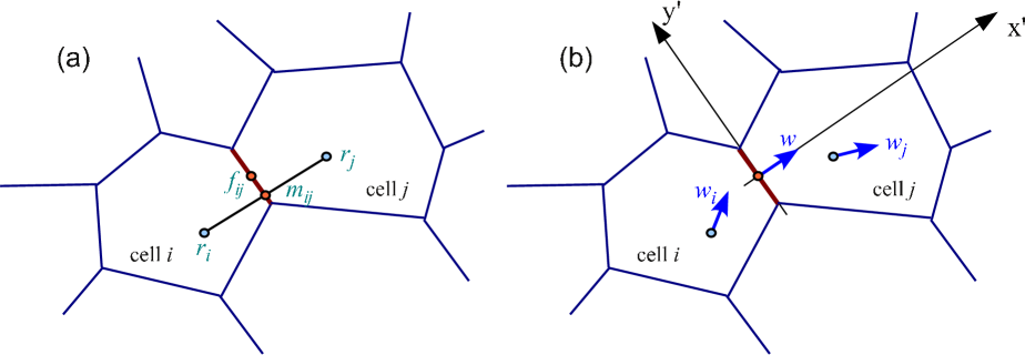
Evidently, a crucial step lies in obtaining a numerical estimate of the fluxes $\vec{{\hat{F}}}_{ij}$. We employ the MUSCL-Hancock scheme (van Leer, 1984; Toro, 1997; van Leer, 2006) already discussed in section 6.7, which is a well-known and relatively simple approach for obtaining second-order accuracy in space and time. This scheme is used in several state-of-the art Eulerian codes (e.g. Fromang et al., 2006; Mignone et al., 2007; Cunningham et al., 2009). In its basic form, the MUSCL-Hancock scheme involves a slope-limited piece-wise linear reconstruction step within each cell, a first order prediction step for the evolution over half a timestep, and finally a Riemann solver to estimate the time-averaged inter-cell fluxes for the timestep. After the fluxes have been applied to each cell, a new averaged state of the cells is constructed. This sequence of steps in a timestep hence follows the general REA approach.

Figure 31 gives a sketch of the geometry involved in estimating the flux across the face between two Voronoi cells. Truly multidimensional Riemann solvers have been developed recently (Wendroff, 1999; Brio et al., 2001; Balsara, 2010), but it is unclear whether they can be readily adapted to our complicated face geometry. We therefore follow the common approach and calculate the flux for each face separately, treating it as an effectively one-dimensional problem. Since we do not work with Cartesian meshes, we cannot use operating splitting to deal with the individual spatial dimensions, hence we apply an unsplit approach. For defining the Riemann problem normal to a cell face, we rotate the fluid state into a suitable coordinate system with the $x^{\prime}$-axis normal to the cell face (see sketch). This defines the left and right states across the face, which we pass to an (exact) Riemann solver, following Toro (1997). Once the flux has been calculated with the Riemann solver, we transform it back to the lab frame. In order to obtain Galilean-invariance and stable upwind behavior, the Riemann problem needs to be solved in the frame of the moving face.

In the moving-mesh hydrodynamical scheme implemented in the AREPO code (Springel, 2010a), each timestep hence involves the following basic steps:

1. Calculate a new Voronoi tessellation based on the current coordinates $\vec{r}_{i}$ of the mesh generating points. This also gives the centers-of-mass $\vec{s}_{i}$ of each cell, their volumes $V_{i}$, as well as the areas $A_{ij}$ and centers $\vec{f}_{ij}$ of all faces between cells.

2. Based on the vector of conserved fluid variables $\vec{Q}_{i}$ associated with each cell, calculate the ‘primitive’ fluid variables $\vec{W}_{i}=(\rho_{i},\vec{v}_{i},P_{i})$ for each cell.

3. Estimate the gradients of the density, of each of the velocity components, and of the pressure in each cell, and apply a slope-limiting procedure to avoid overshoots and the introduction of new extrema.

4. Assign velocities $\vec{w}_{i}$ to the mesh generating points.

5. Evaluate the Courant criterion and determine a suitable timestep size $\Delta t$.

6. For each Voronoi face, compute the flux $\vec{{\hat{F}}}_{ij}$ across it by first determining the left and right states at the midpoint of the face by linear extrapolation from the cell midpoints, and by predicting these states forward in time by half a timestep. Solve the Riemann problem in a rotated frame that is moving with the speed of the face, and transform the result back into the lab-frame.

7. For each cell, update its conserved quantities with the total flux over its surface multiplied by the timestep, using equation (326). This yields the new state vectors $\vec{Q}_{i}^{(n+1)}$ of the conserved variables at the end of the timestep.

8. Move the mesh-generating points with their assigned velocities for this timestep.

Full details for each of these different steps as well as test problems can be found in Springel (2010a). Recently, a number of science applications involving fairly large calculations with AREPO have been carried out that demonstrate the practical advantages of this technique for applications in galaxy formation and evolution (e.g. Greif et al., 2011a, b; Vogelsberger et al., 2012, 2013, 2014; Marinacci et al., 2014; Pakmor et al., 2014).

9 Parallelization techniques and current computing trends

Modern computer architectures offer ever more computational power that we ideally would like to use to their full extent for scientific purposes, in particular for simulations in astrophysics. However, unlike in the past, the speed of individual compute cores, which may be viewed as serial computers, has recently hardly grown any more (in stark contrast to the evolution a few years back). Instead, the number of cores on large supercomputers has started to increase exponentially. Even on laptops and cell-phones, multi-core computers have become the norm rather than the exception.

However, most algorithms and computer languages are constructed around the concepts of a serial computer, in which a stream of operations is executed sequentially. This is also how we typically think when we write computer code. In order to exploit the power available in modern computers, one needs to change this approach and adopt parallel computing techniques. Due to the large variety of computer hardware, and the many different technical concepts for devising parallel programs, we can only scratch the surface here and make a few basic remarks about parallelization, and some basic techniques that are currently in wide use for it. The interested student is encouraged to read more about this in textbooks and/or in online resources.

9.1 Hardware overview

Let’s start first with a schematic overview over some of the main characteristics and types of current computer architectures.

Serial computer

The traditional model of a computer consists of a central processing unit (CPU), capable of executing a sequential stream of load, store, and compute operations, attached to a random access memory (RAM) used for data storage, as sketched in Fig. 32. Branches and jumps in this stream are possible too, but at any given time, only one operation is carried out. The operating system may still provide the illusion that several programs are executed concurrently, but in this case this is reached by time slicing the single compute resource.

4cm!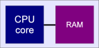

Figure 32: Simple schematic sketch of a serial computer – most traditional computer languages are formulated for this type of machine.

Most computer languages are built around this model; they can be viewed as a means to create the stream of serial operations in a convenient way. One can in principle also by-pass the computer language and write down the machine instructions directly (assembler programming), but fortunately, modern compilers make this unnecessary in scientific applications (except perhaps in very special circumstances where extreme performance tuning is desired).

Multi-core nodes

It is possible to attach multiple CPUs to the same RAM (see Fig. 33), and, especially in recent times, computer vendors have started to add multiple cores to individual CPUs. On each CPU and each core of a CPU, different programs can be executed concurrently, allowing real parallel computations.

4.2cm!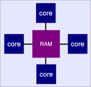

Figure 33: Multi-core computer with shared memory.

In machines with uniform memory access, the individual cores can access the memory with the same speed, at least in principle. In this case the distinction between a CPU and a core can become confusing (and is in fact superfluous at some level), because it is ambiguous whether “CPU” refers to a single core, or all the cores on the same die of silicon (it’s hence best to simple speak about cores to avoid any confusion).

Multi-socket compute nodes

Most powerful compute servers feature these days a so-called NUMA (non-uniform memory access) architecture. Here the full main memory is accessible by all cores, but not all parts of it with the same speed. The compute nodes usually feature individual multi-core CPUs, each with a dedicated memory bank attached (see Fig. 34). Read and write operations to this part of physical memory are fastest, while accessing the other memory banks is typically noticeably slower and often involves going through special, high-bandwidth interprocessor bus systems.

Figure 34: Non-uniform memory access computer. Here multiple sockets contain several processor dies, each with multiple cores. The total memory is split up into banks, which can be accessed with maximum speed by the processor associated with it, and with a reduced speed from different processors.

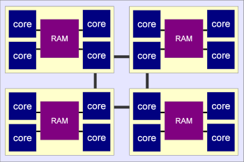
In such machines, maximum compute performance is only reached when the data that is worked on by a core resides on the “right” memory bank. Fortunately, the operating system will normally try to help with this by satisfying memory requests out of the closest part of physical memory, if possible. It is then also advantageous to tell the operating system to “pin” execution of a process or thread to a certain physical core, so that it is not rescheduled to run on another core from which the already allocated data may be accessible only with slower speed.

Compute clusters

Very powerful supercomputers used in the field of high-performance computing (HPC) can be formed by connecting many compute nodes through a fast communication network, as sketched in Figure 35. This can be standard gigabit ethernet in some cases, but usually much faster (and more expensive) communication networks such as infiniband are employed. The leading supercomputers in the world are of this type, and currently typically reach several $10^{5}$ cores in total, with the first machines surpassing even $10^{6}$ cores. Towards the end of the decade, when exaflop machines (capable of carrying out $10^{18}$ floating point operations per second) are expected, this may even grow to $10^{8}$ or beyond. How to use these machines efficiently for interesting science problems, which tend to be tightly coupled and not amenable to unlimited levels of computational concurrency, is however still an unsolved problem.

Figure 35: In large high-performance supercomputers, one typically connects a large number of powerful compute nodes (often of NUMA type) through a very fast dedicated communication network.

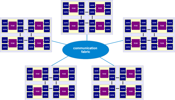
Device computing

A comparatively new trend in scientific computing is to augment classical compute nodes with special accelerator cards that are particularly tuned to floating point calculations. These cards have much simpler, less flexible compute cores, but the transistors saved on implementing chip complexity can be spent on building more powerful compute engines that can execute many floating point operations in parallel. Graphics processing units (GPUs) have been originally developed with such a design just for the vector operations necessary to render graphics, but now their streaming processors can also be used for general purpose calculations. For certain applications, GPUs can be much faster than ordinary CPUs, but programming them is harder.

7.0cm!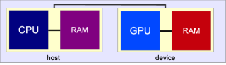

Figure 36: Hybrid compute node. An accelerator device (a GPU, or an Intel Xeon Phi card) is connected to an ordinary compute node through a fast bus system. Usually, host CPU and computing device each have their own RAM.

In so-called hybrid compute nodes (Fig. 36), one has one or several ordinary CPUs coupled to one or several GPUs, or other accelerator cards such as the new Intel Xeon Phi. Of course, these hybrid nodes can be clustered again with a fabric to form powerful supercomputers. In fact, the fastest machines in the world are presently of this type.

Vector cores

Another hardware aspect that should not be overlooked is that single compute cores are actually increasingly capable to carry out so-called vector instructions. Here a single instruction (such as addition, multiplication, etc.) is applied to multiple data elements (a vector). This is also a form of parallelization, allowing the calculation throughput to be raised significantly. Below is an example that calculates $x=a\cdot b$ element by element for 4-vectors $a$ and $b$ using Intel’s Advanced Vector Instructions (AVX). These can be programmed explicitly through intrinsics in C, which are basically individual machine instructions hidden as macros or function calls within C. (Usually, one does not do this manually though, but rather hopes the compiler emits such instructions somehow automatically.)

⬇

1 #include <xmmintrin.h>

2

3 void do_stuff(void)

4 {

5 double a[4], b[4], res[4];

6

7 __m256d x = _mm256_load_pd(a);

8 __m256d y = _mm256_load_pd(b);

9

10 x = _mm256_mul_pd(x, y);

11

12 _mm256_store_pd(res, x);

13 }

The current generation of the x86 processors from Intel/AMD features SSE/AVX instructions that operate on vectors of up to 256 bits. This means that 4 double-precision or 8 single precision operations can be executed with such an instruction, roughly in the same speed that an ordinary double or single-precision operation takes. So if these instructions can be used in an optimum way, one achieves a speed-up by a factor of up to 4 or 8, respectively. On the Intel Xeon Phi chips, the vector length has already doubled again and is now 512 bits, hence allowing another factor of 2 in the performance. Likely, we will see even larger vector lengths in the near future.

Hyperthreading

A general problem in exploiting modern computer hardare to its full capacity is that accessing main memory is very much slower than doing a single floating point operation in a compute core (note that moving data also costs more energy than doing a floating point calculation, which is becoming an important consideration too). As a result, a compute core typically spends a large fraction of its cycles waiting for data to arrive from memory.

The idea of hyperthreading as implemented in CPUs by Intel and in IBM’s Power architecture is to use this wait time by letting the core do some useful work in the meantime. This is achieved by “overloading” the compute core with several execution streams. But instead of letting the operating system toggle between their execution, the hardware itself can switch very rapidly between these different “hyperthreads”. Even though there is still some overhead in changing the execution context from one thread to another, this strategy can still lead to a substantial net increase in the calculational throughput on the core. Effectively, to the operating system and user it appears as if there are more cores (so called virtual cores) than there are real physical cores. For example, the IBM CPU on the Bluegene/Q machine has 16 physical cores with 4-fold hyperthreading, yielding 64 virtual cores. One may then start 64 threads in the user application. Compared with just starting 16 threads, one will then not get four times the performance, but still perhaps 2.1 times the performance or so, depending on the particular application.

9.2 Amdahl’s law

Before we discuss some elementary parallelization techniques, it is worthwhile to point out a fundamental limit to the parallel speed-up that may be reached for a given program. We define the speed up here as the ratio of the total execution time without parallelization (i.e. when the calculation is done in serial) to the total execution time obtained when the parallelization is enabled.

Suppose we have a program that we have successfully parallelized. In practice, this parallelization is never going to be fully perfect. Normally there are parts of the calculation that remain serial, either for algorithmic reasons, due to technical limitations, or we considered them unimportant enough that we have not bothered to parallelize those too. Let us call the residual serial fraction $f_{s}$, i.e. this is the fraction of the execution time spent in the corresponding code parts when the program is executed in ordinary serial mode.

Then Amdahl’s law (Amdahl, 1967) gives the maximum parallel speed up as

$$\mbox{maximum parallel speed up}=\frac{1}{f_{s}}.$$ (327)

This is simply because in the most optimistic case we can at most assume that our parallelization effort has been perfect, so that the time spent in the parallel parts approaches zero for a sufficiently large number of cores. The serial time remains unaffected by this, however, and does not shrink at all. The lesson is a bit sobering: Achieving large parallel speed-ups, say beyond a factor of 100 or so, also requires extremely tiny residual serial fractions. This is sometimes very hard to reach in practice, and for certain problems, it may even be impossible.

9.3 Shared memory parallelization

Shared memory parallelization can be used to distribute a computational work-load on the multiple available compute cores that have access to the same memory, which is where the data resides. UNIX processes are isolated from each other – they usually have their own protected memory, preventing simple joint work on the same memory space (data exchange requires the use of files, sockets, or special devices such as /dev/shm). But, a process may be split up into multiple execution paths, called threads. Such threads share all the resources of the parent process (memory, files, etc.), and they are the ideal vehicle for efficient shared memory parallelization.

Threads can be created and destroyed manually, e.g. with the pthreads-libary of the POSIX standard. Here is a simple example how this could be achieved:

⬇

1 #include <pthread.h>

2

3 void do_stuff(void)

4 {

5 int i, threadid = 1;

6 pthread_attr_r attr;

7 pthread_t mythread;

8 pthread_attr_init(&attr);

9 pthread_create(mythread, &attr, evaluate, &threadid);

10

11 for(i = 0; i < 100; i++)

12 some_expensive_calculation(i);

13 }

14

15 void *evaluate(void *p)

16 {

17 int i;

18

19 for(i = 100; i < 200; i++)

20 some_expensive_calculation(i);

21 }

Here the two loops in lines 11/12 and 19/20 will be carried out simultaneously (i.e. in parallel) by two different threads of the same parent process. While certainly doable in principle this style of parallel programming is a bit cumbersome if one has to do it regularly – fortunately, there is a convenient alternative (see below) where much of the thread logistics is carried out by the compiler.

OpenMP and its fork-join model

A simpler approach for shared memory programming is to use the OpenMP standard, which is a language/compiler extension for C/C++ and Fortran. It allows the programmer to give simple hints to the compiler, instructing it which parts can be executed in parallel sections. OpenMP then automatically deals with the thread creation and destruction, and completely hides this nuisance from the programmer. As a result, it becomes possible to parallelize a code with minimal modifications, and the modified program can still be compiled and executed without OpenMP as a serial code. Here is how the example from above would like like in OpenMP:

⬇

1 #include <omp.h>

2

3 void do_stuff(void)

4 {

5 int i;

6

7 #pragma omp parallel for

8 for(i = 0; i < 200; i++)

9 some_expensive_calculation(i);

10 }

This is obviously a lot simpler. We see here an example of so-called loop-level parallelism with OpenMP. In practice, one simply puts a special directive for the compiler in front of the loop. That’s basically all. The OpenMP compiler will then automatically wake up all available threads at the beginning of the loop (the “fork”), it will then distribute the loop iterations evenly onto the different threads, and they are then executed concurrently. Finally, once all loop iterations have completed, the threads are put to sleep again, and only the master thread continues in serial fashion. Note that this will only work correctly if there are no dependencies between the different loop iterations, or in other words, the order in which they are carried out needs to be unimportant. If everything goes well, the loop is then executed faster by a factor close to the number of threads.

This illustrates the central idea of OpenMP, which is to let the programmer identify sections in a code that can be executed in parallel and annotate these to the compiler. Whenever such a section is encountered, the program execution is split into a number of threads that work in a team in parallel on the work of the section. Often, this work is a simple loop whose iterations are distributed evenly on the team, but also more general parallel sections are possible. At the end of the parallel section, the threads join again onto the master thread, the team is dissolved, and serial execution resumes until the next parallel section starts. Normally, the number of threads used in each parallel section is constant, but this can also be changed through calls of OpenMP runtime library functions. In order for this to work in practice, one has to do a few additional things:

• The code has to be compiled with an OpenMP capable compiler. This feature often needs to be enabled with a special switch, e.g. with gcc,

      gcc -fopenmp ...
  

  needs to be used.

• For some more advanced OpenMP features accessible through calls of OpenMP-library functions, one should include the OpenMP header file

      #include <omp.h>
  

• In order to set the number of threads that are used, one should set the OMP _NUM_THREADS environment variable before the program is started. Depending on the shell that is used (here bash is assumed), this can be done for example through

      export OMP_NUM_THREADS=8
  

  in which case 8 threads would be allocated by OpenMP. Normally one should then also have at least eight (virtual) cores available. The omp_get_num_

threads() function call can be used inside a program to check how many threads are available.

Race conditions

When OpenMP is used, one can easily create hideous bugs if different threads are allowed to modify the same variable at the same time. Which thread wins the “race” and gets to modify a variable first is essentially undetermined in OpenMP (note that the exact timings on a compute core can vary stochastically due to “timing noise” originating in interruptions from the operating system), so that subsequent executions may each time yield a different result and seemingly produce non-deterministic behavior. A simple example for incorrect code with this problem is the following double-loop:

⬇

1 int i, j;

2 #pragma omp parallel for

3 for(i = 0; i < N; i++)

4 {

5 for(j = 0; j < N; j++)

6 {

7 do_stuff(i, j);

8 }

9 }

Here the simple OpenMP directive in the outer loop will instruct the i-loop to be split up between different threads. However, there is only one variable for j, shared by all the threads. They are hence not able to carry out the inner loop independent from each other! What is needed here is that each thread gets its own copy of j, so that the inner loop can be executed independently. This can be achieved by either adding a private(j) clause to the OpenMP directive of the outer loop, like this:

⬇

1 int i;

2 #pragma omp parallel for private(j)

3 for(i = 0; i < N; i++)

4 {

5 for(j = 0; j < N; j++)

6 {

7 do_stuff(i, j);

8 }

9 }

or by exploiting the scoping rules of C for the variable j, declaring it in the loop body:

⬇

1 int i;

2 #pragma omp parallel for

3 for(i = 0; i < N; i++)

4 {

5 int j;

6 for(j = 0; j < N; j++)

7 {

8 do_stuff(i, j);

9 }

10 }

Reductions

Another common construct in code are reductions that build, e.g., large sums or products, such as attempted incorrectly in this example:

⬇

1 int count = 0;

2 #pragma omp parallel for

3 for(i = 0; i < N; i++)

4 {

5 if(complicated_calculation(i) > 0)

6 count++;

7 }

Again, even though here the loop is nicely parallelized by OpenMP, we may nevertheless get an incorrect result for count. This is because the increment of this variable is not necessarily carried out as a single instruction. It basically involves a read from memory, an addition of 1, and a write back. If now two threads happen to arrive at this statement at essentially the same time, they will both read count, increment it, and then write it back. But in this case the variable will end up being incremented only by one unit and not by two, because one of the threads is ignorant of the change of count by the other and overwrites it. We have here another example for a race conditions.

There are different solutions to this problem. One is to serialize the increment of count by putting a so-called lock around it. Since we here have a simple increment of a variable, a particularly fast look – a so-called atomic instruction – is possible. This can be done through:

⬇

1 int count = 0;

2 #pragma omp parallel for

3 for(i = 0; i < N; i++)

4 {

5 if(complicated_calculation(i) > 0)

6 {

7 #pragma omp atomic

8 count++;

9 }

10 }

But this can still cost substantial performance: If one or several threads arrive at the statement protected by the atomic lock at the same time, they have to wait and do the operation one after the other.

A better solution would be to have private variables for count for each thread, and only at the end of the parallel section add up the different copies to get the global sum. OpenMP can generate the required code automatically, all that is needed is to add the clause reduction(+:count) to the directive for parallelizing the loop:

⬇

1 int count = 0;

2 #pragma omp parallel for reduction(+:count)

3 for(i = 0; i < N; i++)

4 {

5 if(complicated_calculation(i) > 0)

6 count++;

7 }

This shall suffice for giving a flavor of the style and the concepts of OpenMP. A more detailed description of the OpenMP standard can for example be found in various textbooks, and good online tutorials.

9.4 Distributed memory parallelization with MPI

To use multiple nodes in compute clusters, OpenMP is not sufficient. Here one either has to use special programming languages that directly support distributed memory models (for example UPC, Co-Array Fortran, or Chapel), or one turns to the “Message Passing Interface” (MPI). MPI has become the de-facto standard for programming large-scale simulation code.

MPI offers library functions for exchanging messages between different processes running on the same or different compute nodes. The compute nodes do not necessarily have to be physically close, in principle they can also be loosely connected over the internet (although for tightly coupled problems the message latency makes this unattractive). Most of the time, the same program is executed on all compute cores (SPMD, “single program multiple data”), but they operate on different data such that the computational task is put onto many shoulders and a parallel speed up is achieved. Since the MPI processes are isolated from each other, all data exchanges necessary for the computations have to be explicitly programmed – this makes this approach much harder than, e.g., OpenMP. Often substantial program modifications and algorithmic changes are needed for MPI.

Once a program has been parallelized with MPI, it may also be augmented with OpenMP. Such hybrid parallel code may then be executed in different ways on a cluster. For example, if one has two compute nodes with 8 cores each, one could run the program with 16 MPI tasks, or with 2 MPI tasks that each using 8 OpenMP threads, or with 4 MPI tasks and 4 OpenMP threads each. It would not make sense to use 1 MPI task and 16 OpenMP threads, however – then only one of the two compute nodes could be used.

General structure of an MPI program

A basic template of a simple MPI program in C looks as follows:

⬇

1 #include <mpi.h>

2

3 int main(int argc, char **argv)

4 {

5 MPI_Init(&argc, &argv);

6 .

7 .

8 /* now we can send/receive message to other MPI ranks */

9 .

10 .

11 MPI_Finalize();

12 }

• To compile this program, one would normally use a compiler wrapper, for example mpicc instead of cc, which sets pathnames correctly such that the MPI header files and MPI library files are found by the compiler.

• For executing the MPI program, one will normally use a start-up program such as mpirun or mpiexec. For example, the command

    mpirun -np 8 ./mycalc
  

  could be used to launch 8 instances of the program mycalc.

If a normal serial program is augmented by MPI_Init in the above fashion, and if it is started multiple times with mpirun -np X, it will simply do multiple times exactly the same thing as the corresponding serial program (unless they somehow synchronize their work through modifying common files). To change this behavior and achieve non-trivial parallelism, the execution paths taken in each copy of the program need to become different. This is normally achieved by making it explicitly depend on the rank of the MPI task. All the $N$ processes of an MPI program form a so-called communicator, and they are labelled with a unique rank-id, with the values $0$, $1$, $2$, $\ldots$, $N-1$. MPI processes can then send and receive message from different ranks using these IDs to identify each other.

The first thing an MPI program normally does is therefore to find out how many MPI processes there are in the “world”, and what the rank of the current instance of the program is. This is done with the function calls

⬇

1 int NTask, ThisTask;

2

3 MPI_Comm_size(MPI_COMM_WORLD, &NTask);

4 MPI_Comm_rank(MPI_COMM_WORLD, &ThisTask);

The returned integers NTask and ThisTask then contain the number of MPI tasks and the rank of the current one, respectively.

A simple point to point message

With this information in hand, we can then exchange simple messages between two different MPI ranks. For example, a send of a message consisting of 50 integers from rank 5 to rank 7 could be programmed like this:

⬇

1 int data[50], result[50]

2

3 if(ThisTask == 5)

4 MPI_Send(data, 50, MPI_INT, // buffer, size, type

5 7, 12345, // destination, message tag

6 MPI_COMM_WORLD); // communicator id

7

8 if(ThisTask == 7)

9 MPI_Recv(result, 50, MPI_INT, // buffer, size, type

10 5, 12345, // destination, message tag

11 MPI_COMM_WORLD, MPI_STATUS_IGNORE); //id, status

Here one sees the general structure of most send/recv calls, which always decompose a message into an “envelope” and the “data”. The envelope describes the rank-id of sender/receiver, the size and type of the message, and a user-specified tag (this is the ‘12345’ here), which can be used to distinguish messages of the same length.

Through the if-statements that depend on the local MPI rank, different execution paths for sender and receiver are achieved in this example. Note that if something goes wrong here, for example an MPI rank posts a receive but the matching send does not occur, the program will deadlock, where one or several of the MPI tasks gets stuck in waiting in vain for messages that are not sent. This is one of the many new types of bugs one has to cope with in distributed parallel programs.

It is also possible to make MPI communications non-blocking and achieve asynchronous communication in this way. The MPI-2 standard even contains some calls for one-sided communication operations that do not always require direct involvement of both the sending and receiving sides.

Collective communications

The MPI standard knowns a large number of functions that can be used to conveniently make use of commonly encountered communication patterns. For example, there are calls for broadcasts which send the same data to all other MPI tasks in the same communicator. There are also gather and scatter operations that collect data elements from all tasks, or distribute them as disjoint sets to the other tasks. Finally, there are reduction function that allow one to conveniently calculate sums, minima, maxima, etc., over variables held by all MPI tasks in a communicator.

A detailed description of all these possibilities is way passed the scope of these brief lecture notes. Please check out a textbook (e.g. Pacheco, 1997) or some of the online resources on MPI if you want to get detailed information about MPI and start to program in it.

References

- Agertz et al. (2007) Agertz, O., Moore, B., Stadel, J., Potter, D., Miniati, F., Read, J., Mayer, L., Gawryszczak, A., Kravtsov, A., et al.Nordlund, Å., Pearce, F., Quilis, V., Rudd, D., Springel, V., Stone, J., Tasker, E., Teyssier, R., Wadsley, J., & Walder, R. 2007, MNRAS, 380, 963
- Amdahl (1967) Amdahl, G. M. 1967, in Proceedings of the April 18-20, 1967, Spring Joint Computer Conference, AFIPS ’67 (Spring) (New York, NY, USA: ACM), 483–485
- Atkinson (1978) Atkinson, K. 1978, An introduction to numerical analysis (Wiley)
- Bagla (2002) Bagla, J. S. 2002, Journal of Astrophysics and Astronomy, 23, 185
- Balsara (2010) Balsara, D. S. 2010, Journal of Computational Physics, 229, 1970
- Balsara et al. (2009) Balsara, D. S., Rumpf, T., Dumbser, M., & Munz, C.-D. 2009, Journal of Computational Physics, 228, 2480
- Barnes & Hut (1986) Barnes, J. & Hut, P. 1986, Nature, 324, 446
- Bauer & Springel (2012) Bauer, A. & Springel, V. 2012, MNRAS, 423, 2558
- Bertone et al. (2005) Bertone, G., Hooper, D., & Silk, J. 2005, Phys. Rep., 405, 279
- Binney & Tremaine (1987) Binney, J. & Tremaine, S. 1987, Galactic dynamics (Princeton University Press)
- Binney & Tremaine (2008) —. 2008, Galactic Dynamics: Second Edition (Princeton University Press)
- Brandt (1977) Brandt, A. 1977, Mathematics of Computation, 31, 333
- Braun & Sambridge (1995) Braun, J. & Sambridge, M. 1995, Nature, 376, 655
- Briggs et al. (2000) Briggs, W. L., Henson, V. E., & McCormick, S. F. 2000, A Multigrid Tutorial, EngineeringPro collection (Society for Industrial and Applied Mathematics (SIAM, Philadelphia))
- Brio et al. (2001) Brio, M., Zakharian, A. R., & Webb, G. M. 2001, Journal of Computational Physics, 167, 177
- Campbell (1897) Campbell, J. E. 1897, Proc Lond Math Soc, 28, 381
- Chandrasekhar (1943) Chandrasekhar, S. 1943, ApJ, 97, 255
- Cooley & Tukey (1965) Cooley, J. W. & Tukey, J. W. 1965, Math. Comp., 19, 297
- Courant et al. (1928) Courant, R., Friedrichs, K., & Lewy, H. 1928, Mathematische Annalen, 100, 32
- Cullen & Dehnen (2010) Cullen, L. & Dehnen, W. 2010, MNRAS, 408, 669
- Cunningham et al. (2009) Cunningham, A. J., Frank, A., Varnière, P., Mitran, S., & Jones, T. W. 2009, ApJS, 182, 519
- Dehnen (2000) Dehnen, W. 2000, ApJ, 536, L39
- Dehnen (2002) —. 2002, Journal of Computational Physics, 179, 27
- Dehnen & Aly (2012) Dehnen, W. & Aly, H. 2012, MNRAS, 425, 1068
- Diniz et al. (2002) Diniz, P., da Silva, E., & Netto, S. 2002, Digital Signal Processing: System Analysis and Design (Cambridge University Press)
- Dolag et al. (2005) Dolag, K., Vazza, F., Brunetti, G., & Tormen, G. 2005, MNRAS, 364, 753
- Dubois et al. (2014) Dubois, Y., Pichon, C., Welker, C., Le Borgne, D., Devriendt, J., Laigle, C., Codis, S., Pogosyan, D., Arnouts, S., Benabed, K., Bertin, E., Blaizot, J., Bouchet, F., Cardoso, J.-F., Colombi, S., de Lapparent, V., Desjacques, V., Gavazzi, R., Kassin, S., Kimm, T., McCracken, H., Milliard, B., Peirani, S., Prunet, S., Rouberol, S., Silk, J., Slyz, A., Sousbie, T., Teyssier, R., Tresse, L., Treyer, M., Vibert, D., & Volonteri, M. 2014, ArXiv e-prints: 1402.1165
- Eckart (1960) Eckart, C. 1960, Physics of Fluids, 3, 421
- Field (1965) Field, G. B. 1965, ApJ, 142, 531
- Frenk et al. (1999) Frenk, C. S., White, S. D. M., Bode, P., Bond, J. R., Bryan, G. L., Cen, R., Couchman, H. M. P., Evrard, A. E., Gnedin, N., Jenkins, A., Khokhlov, A. M., Klypin, A., Navarro, J. F., Norman, M. L., Ostriker, J. P., Owen, J. M., Pearce, F. R., Pen, U.-L., Steinmetz, M., Thomas, P. A., Villumsen, J. V., Wadsley, J. W., Warren, M. S., Xu, G., & Yepes, G. 1999, ApJ, 525, 554
- Fromang et al. (2006) Fromang, S., Hennebelle, P., & Teyssier, R. 2006, A&A, 457, 371
- Gauss (1866) Gauss, C. F. 1866, Nachlass: Theoria interpolationis methodo nova tractata (Earl Friedrich Gauss, Werke, Band 3, Gottingen: Koniglichen Gesellschaft der Wissenschaften), pp. 265–303
- Gingold & Monaghan (1977) Gingold, R. A. & Monaghan, J. J. 1977, MNRAS, 181, 375
- Gnedin (1995) Gnedin, N. Y. 1995, ApJS, 97, 231
- Goldstein (1950) Goldstein, H. 1950, Classical mechanics (Addison-Wesley)
- Greif et al. (2011a) Greif, T. H., Springel, V., White, S. D. M., Glover, S. C. O., Clark, P. C., Smith, R. J., Klessen, R. S., & Bromm, V. 2011a, ApJ, 737, 75
- Greif et al. (2011b) Greif, T. H., White, S. D. M., Klessen, R. S., & Springel, V. 2011b, ApJ, 736, 147
- Hairer et al. (2002) Hairer, E., Lubich, C., & Wanner, G. 2002, Geometric numerical integration, Springer Series in Computational Mathematics (Springer, Berlin)
- Harten et al. (1983) Harten, A., Lax, P. D., & Van Leer, B. 1983, SIAM Review, 25, 35
- Hassan et al. (1998) Hassan, O., Probert, E. J., & Morgan, K. 1998, International Journal for Numerical Methods in Fluids, 27, 41
- Hernquist (1987) Hernquist, L. 1987, ApJS, 64, 715
- Hernquist et al. (1991) Hernquist, L., Bouchet, F. R., & Suto, Y. 1991, ApJS, 75, 231
- Hernquist et al. (1993) Hernquist, L., Hut, P., & Makino, J. 1993, ApJ, 402, L85
- Hernquist & Katz (1989) Hernquist, L. & Katz, N. 1989, ApJS, 70, 419
- Hockney & Eastwood (1988) Hockney, R. W. & Eastwood, J. W. 1988, Computer simulation using particles (Bristol: Hilger)
- Hopkins (2013) Hopkins, P. F. 2013, MNRAS, 428, 2840
- Hu et al. (2014) Hu, C.-Y., Naab, T., Walch, S., Moster, B. P., & Oser, L. 2014, ArXiv e-prints: 1402.1788
- James (1977) James, R. A. 1977, Journal of Computational Physics, 25, 71
- Kirkwood (1946) Kirkwood, J. G. 1946, J. Chem. Phys., 14, 180
- Klypin & Shandarin (1983) Klypin, A. A. & Shandarin, S. F. 1983, MNRAS, 204, 891
- Knebe et al. (2001) Knebe, A., Green, A., & Binney, J. 2001, MNRAS, 325, 845
- Kolmogorov (1941) Kolmogorov, A. N. 1941, Proceedings of the USSR Academy of Sciences, 32, 16
- Landau & Lifshitz (1959) Landau, L. D. & Lifshitz, E. M. 1959, Fluid mechanics (Course of theoretical physics, Oxford: Pergamon Press)
- LeVeque (2002) LeVeque, R. J. 2002, Finite volume methods for hyperbolic systems (Cambridge University Press)
- Lucy (1977) Lucy, L. B. 1977, AJ, 82, 1013
- Makino et al. (2003) Makino, J., Fukushige, T., Koga, M., & Namura, K. 2003, PASJ, 55, 1163
- Marinacci et al. (2014) Marinacci, F., Pakmor, R., & Springel, V. 2014, MNRAS, 437, 1750
- Mavriplis (1997) Mavriplis, D. J. 1997, Annual Review of Fluid Mechanics, 29, 473
- Mignone et al. (2007) Mignone, A., Bodo, G., Massaglia, S., Matsakos, T., Tesileanu, O., Zanni, C., & Ferrari, A. 2007, ApJS, 170, 228
- Mitchell et al. (2009) Mitchell, N. L., McCarthy, I. G., Bower, R. G., Theuns, T., & Crain, R. A. 2009, MNRAS, 395, 180
- Miyoshi & Kusano (2005) Miyoshi, T. & Kusano, K. 2005, Journal of Computational Physics, 208, 315
- Mo et al. (2010) Mo, H., van den Bosch, F. C., & White, S. 2010, Galaxy Formation and Evolution (Cambridge University Press)
- Monaghan (1992) Monaghan, J. J. 1992, ARA&A, 30, 543
- Morris (1997) Morris, J. 1997, Journal of Computational Physics, 136, 41
- Ollivier-Gooch (1997) Ollivier-Gooch, C. F. 1997, Journal of Computational Physics, 133, 6
- Pacheco (1997) Pacheco, P. S. 1997, Parallel Programming with MPI (Morgan Kaufmann Publishers, San Francisco)
- Pakmor et al. (2014) Pakmor, R., Marinacci, F., & Springel, V. 2014, ApJ, 783, L20
- Peacock (1999) Peacock, J. A. 1999, Cosmological Physics (Cambridge University Press)
- Pelupessy et al. (2003) Pelupessy, F. I., Schaap, W. E., & van de Weygaert, R. 2003, A&A, 403, 389
- Pen (1998) Pen, U.-L. 1998, ApJS, 115, 19
- Pope (2000) Pope, S. B. 2000, Turbulent Flows (Cambridge University Press)
- Power et al. (2003) Power, C., Navarro, J. F., Jenkins, A., Frenk, C. S., White, S. D. M., Springel, V., Stadel, J., & Quinn, T. 2003, MNRAS, 338, 14
- Press et al. (1992) Press, W. H., Teukolsky, S. A., Vetterling, W. T., & Flannery, B. P. 1992, Numerical recipes in C. The art of scientific computing (Cambridge: University Press, 1992, 2nd ed.)
- Price (2008) Price, D. J. 2008, Journal of Computational Physics, 227, 10040
- Price (2012) Price, D. J. 2012, in Astronomical Society of the Pacific Conference Series, Vol. 453, Advances in Computational Astrophysics: Methods, Tools, and Outcome, ed. R. Capuzzo-Dolcetta, M. Limongi, & A. Tornambè, 249
- Pringle & King (2007) Pringle, J. E. & King, A. 2007, Astrophysical Flows (Cambridge University Press)
- Rankine (1870) Rankine, W. J. M. 1870, Philosophical Transactions of the Royal Society of London, 160, 277–288
- Read & Hayfield (2012) Read, J. I. & Hayfield, T. 2012, MNRAS, 422, 3037
- Read et al. (2010) Read, J. I., Hayfield, T., & Agertz, O. 2010, MNRAS, 405, 1513
- Renardy & Rogers (2004) Renardy, M. & Rogers, R. 2004, An Introduction to Partial Differential Equations, Texts in Applied Mathematics (Springer)
- Rosswog (2005) Rosswog, S. 2005, ApJ, 634, 1202
- Runge (1895) Runge, C. 1895, Math. Ann., 46, 167
- Rusanov (1961) Rusanov, V. V. 1961, J. Comput. Math. Phys. USSR, 1, 267
- Saad (2003) Saad, Y. 2003, Iterative Methods for Sparse Linear Systems: Second Edition (Society for Industrial and Applied Mathematics)
- Saha & Tremaine (1992) Saha, P. & Tremaine, S. 1992, AJ, 104, 1633
- Salmon & Warren (1994) Salmon, J. K. & Warren, M. S. 1994, J. Comp. Phys., 111, 136
- Shu (1992) Shu, F. H. 1992, The physics of astrophysics. Volume II: Gas dynamics. (University Science Books, Mill Valley, CA)
- Springel (2005) Springel, V. 2005, MNRAS, 364, 1105
- Springel (2010a) —. 2010a, MNRAS, 401, 791
- Springel (2010b) —. 2010b, ARA&A, 48, 391
- Springel & Hernquist (2002) Springel, V. & Hernquist, L. 2002, MNRAS, 333, 649
- Springel et al. (2001) Springel, V., Yoshida, N., & White, S. D. M. 2001, New Astronomy, 6, 79
- Stadel (2001) Stadel, J. G. 2001, PhD thesis, University of Washington
- Stoer & Bulirsch (2002) Stoer, J. & Bulirsch, R. 2002, Introduction to Numerical Analysis, Texts in Applied Mathematics (Springer)
- Stone et al. (2008) Stone, J. M., Gardiner, T. A., Teuben, P., Hawley, J. F., & Simon, J. B. 2008, ApJS, 178, 137
- Strang (1968) Strang, G. 1968, SIAM J. Numer. Anal., 5, 506
- Tasker et al. (2008) Tasker, E. J., Brunino, R., Mitchell, N. L., Michielsen, D., Hopton, S., Pearce, F. R., Bryan, G. L., & Theuns, T. 2008, MNRAS, 390, 1267
- Teyssier (2002) Teyssier, R. 2002, A&A, 385, 337
- Toro (1997) Toro, E. 1997, Riemann solvers and numerical methods for fluid dynamics (Springer)
- Trac & Pen (2004) Trac, H. & Pen, U.-L. 2004, New Astronomy, 9, 443
- van de Weygaert (1994) van de Weygaert, R. 1994, A&A, 283, 361
- van de Weygaert & Schaap (2009) van de Weygaert, R. & Schaap, W. 2009, in Lecture Notes in Physics, Berlin Springer Verlag, Vol. 665, Data Analysis in Cosmology, ed. V. J. Martínez, E. Saar, E. Martínez-González, & M.-J. Pons-Bordería, 291–413
- van Leer (1984) van Leer, B. 1984, SIAM J. Sci. Stat. Comput., 5, 1
- van Leer (2006) —. 2006, Communications in Computational Physics, 1, 192
- Vogelsberger et al. (2013) Vogelsberger, M., Genel, S., Sijacki, D., Torrey, P., Springel, V., & Hernquist, L. 2013, MNRAS, 436, 3031
- Vogelsberger et al. (2014) Vogelsberger, M., Genel, S., Springel, V., Torrey, P., Sijacki, D., Xu, D., Snyder, G., Bird, S., Nelson, D., & Hernquist, L. 2014, Nature, 509, 177
- Vogelsberger et al. (2012) Vogelsberger, M., Sijacki, D., Kereš, D., Springel, V., & Hernquist, L. 2012, MNRAS, 425, 3024
- Wadsley et al. (2004) Wadsley, J. W., Stadel, J., & Quinn, T. 2004, New Astronomy, 9, 137
- Wadsley et al. (2008) Wadsley, J. W., Veeravalli, G., & Couchman, H. M. P. 2008, MNRAS, 387, 427
- Wendroff (1999) Wendroff, B. 1999, Computers & Mathematics with Applications, 38, 175
- White et al. (1983) White, S. D. M., Frenk, C. S., & Davis, M. 1983, ApJ, 274, L1
- Whitehurst (1995) Whitehurst, R. 1995, MNRAS, 277, 655
- Xu (1995) Xu, G. 1995, ApJS, 98, 355
- Xu (1997) —. 1997, MNRAS, 288, 903