Minimum Core Masses for Giant Planet Formation With Realistic Equations of State and Opacities

Abstract

Giant planet formation by core accretion requires a core that is sufficiently massive to trigger runaway gas accretion in less that the typical lifetime of protoplanetary disks. We explore how the minimum required core mass, $M_{\rm crit}$, depends on a non-ideal equation of state and on opacity changes due to grain growth, across a range of stellocentric distances from 5-100 AU. This minimum $M_{\rm crit}$ applies when planetesimal accretion does not substantially heat the atmosphere. Compared to an ideal gas polytrope, the inclusion of molecular hydrogen (H₂) dissociation and variable occupation of H₂ rotational states increases $M_{\rm crit}$. Specifically, $M_{\rm crit}$ increases by a factor of $\sim$$2$ if the H₂ spin isomers, ortho- and parahydrogen, are in thermal equilibrium, and by a factor of $\sim$$2-4$ if the ortho-to-para ratio is fixed at 3:1. Lower opacities due to grain growth reduce $M_{\rm crit}$. For a standard disk model around a Solar mass star, we calculate $M_{\rm crit}\sim 8M_{\oplus}$ at 5 AU, decreasing to $\sim$$5M_{\oplus}$ at 100 AU, for a realistic EOS with an equilibrium ortho-to-para ratio and for grain growth to cm-sizes. If grain coagulation is taken into account, $M_{\rm crit}$ may further reduce by up to one order of magnitude. These results for the minimum critical core mass are useful for the interpretation of surveys that find exoplanets at a range of orbital distances.

1. Introduction

Core accretion — a prominent theory of giant planet formation — stipulates that Jupiter-sized planets form when planetesimal accretion produces a solid core large enough to attract a massive atmosphere (e.g., Mizuno et al. 1978, Stevenson 1982, Bodenheimer & Pollack 1986, Wuchterl 1993, D’Angelo et al. 2011). Because protoplanetary disks dissipate on timescales of a few Myrs (e.g., Jayawardhana et al., 1999), cores must grow quickly to accrete disk gas. Fast growth is particularly challenging far from a core’s host star, where dynamical times are long. Understanding whether core accretion can work in the outer disk may provide valuable insights into the formation of wide-separation planets such as the directly-imaged giants orbiting HR 8799 (Marois et al., 2008).

Production of such planets in situ by core accretion requires faster core growth rates than typically assumed. However, even if fast growth could be achieved, it produces an additional difficulty. Though the minimum, or critical, core mass to form a giant planet is often quoted as $M_{\rm crit}\sim 10M_{\oplus}$, the actual value depends on how quickly the core accretes planetesimals (e.g., Pollack et al. 1996, Ikoma et al. 2000, Rafikov 2006). Fast accretion heats a core’s atmosphere, increasing pressure support and hence $M_{\rm crit}$. Rafikov (2011) finds that beyond 40-50 AU, a core cannot reach $M_{\rm crit}$ while accreting at the rate it requires to grow during its host disk’s lifetime.

This limit on the distance at which core accretion operates may be overcome if core growth does not proceed at a constant rate. Time-dependent models (e.g., Pollack et al., 1996; Ikoma et al., 2000) suggest that a planets’s feeding zone may be depleted of planetesimals before disk dissipation, causing core growth to stall. Planetesimal accretion no longer deposits energy into the atmosphere which, without this balance for radiative losses, cannot maintain a steady state. The envelope accretes gas while undergoing Kelvin-Helmholtz (KH) contraction. In this regime, a core of any mass would evolve into a giant planet if given an infinite amount of time. In practice, a core produces a giant planet if it has enough time to accumulate an atmosphere of approximately its own mass before its host disk dissipates. The minimum core mass satisfying this criterion is $M_{\rm crit}$.

Because extra heating increases an atmosphere’s pressure, opposing runaway envelope growth, $M_{\rm crit}$ is smallest in the absence of planetesimal accretion. While $M_{\rm crit}$ has been systematically computed as a function of disk properties and stellocentric separation for steady-state atmospheres heated by planetesimal accretion (Rafikov, 2006), no equivalent systematic study is available for this minimum value of $M_{\rm crit}$.

In Piso & Youdin (2014, hereafter Paper I) and this paper, we provide such a systematic study. Given a fiducial disk model, we calculate the $M_{\rm crit}$ required to nucleate runaway atmospheric growth for a fully formed—and no longer accreting—core. We model the planet’s evolution using a series of quasi-static two-layer atmospheres embedded in a protoplanetary disk. Here, we build on the results of Paper I by making two important additions: (1) a realistic equation of state (EOS), and (2) realistic dust opacities. Our aim is twofold: (1) to explain how hydrogen and helium’s non-ideal EOS affects atmospheric growth when compared to an ideal gas, and (2) to provide realistic estimates for the minimum critical core mass required to form a giant planet over a range of semimajor axes.

1.1. Equation of State

We use the EOS of hydrogen and helium mixtures calculated by Saumon et al. (1995), which captures non-ideal effects such as dissociation, ionization, and selective occupation of quantum states at low temperatures. We extend these tables to the very low temperatures and pressures required for planets forming in the outer regions of disks (Appendix A). The EOS tables from Saumon et al. (1995) have often been used to model the interiors of giant planets (e.g., Pollack et al. 1996, Ikoma et al. 2000, Alibert et al. 2005, Hubickyj et al. 2005, Papaloizou & Nelson 2005, Mordasini et al. 2012), as well as in complex stellar evolution simulations involving low temperatures (e.g., Paxton et al. 2011, Paxton et al. 2013, which use the code MESA). More recent EOS tables (Nettelmann et al. 2008, Nettelmann et al. 2012, Militzer & Hubbard 2013) are based on ab initio molecular dynamics simulations and thus avoid some of the approximations of the Saumon et al. (1995) semi-analytical approach. However, though these newer tables are sufficient to model the internal structures of Jupiter and of close-in extrasolar planets, they do not extend to the low temperatures and pressures required for wide-separation planets ($T\lesssim 500$ K, $P\lesssim 1$ GPa, e.g. Militzer & Hubbard 2013). Moreover, the Militzer & Hubbard (2013) EOS tables and the Saumon et al. (1995) tables are in good agreement for entropies, $S$, such that $\log_{10}(S)\gtrsim 8.75$ erg g^-1 K^-1. All models presented here satisfy this constraint.

1.2. Opacity

Opacities in protoplanetary disks are unlikely to be interstellar, and are lowered by grain growth and dust settling. Numerous studies have demonstrated that atmospheric evolution depends strongly on opacity—lower opacities accelerate envelope growth and reduce $M_{\rm crit}$. For example, the analytic model of Stevenson (1982) showed that $M_{\rm crit}\propto\kappa^{3/4}$ for a fully radiative envelope with constant opacity $\kappa$. A series of more modern studies conclude that: Jupiter may have formed in 1 Myr with a core of $10M_{\oplus}$ for an opacity arbitrarily reduced to 2% of the interstellar value (Hubickyj et al., 2005); $M_{\rm crit}$ for Jupiter may be as low as $\sim$$1M_{\oplus}$ for a grain free envelope (Hori & Ikoma, 2010); and the use of grain opacities that take into account coagulation and settling reduces the formation time for Jupiter by up to 80% (Movshovitz et al., 2010). A recent study by Mordasini et al. (2014) investigates the effect of opacity on the formation of populations of synthetic planets, and finds from comparisons with observations that opacities are likely to be much smaller than interstellar. Lastly, Paper I shows that reducing the opacity from interstellar to 1% of interstellar reduces $M_{\rm crit}$ by a factor of $\sim$$2$.

Thus, to provide realistic estimates for $M_{\rm crit}$, we must employ realistic opacities. For temperatures below dust sublimation, we employ opacity tables from D’Alessio et al. (2001), which are used to model observations of protoplanetary disks. We present results for both a standard collisional cascade grain size distribution and for a shallower distribution, appropriate for coagulation (see Section 5 for details). At high temperatures, where dust sublimates, we employ the analytic opacity law of Bell & Lin (1994). For our purposes, this expression sufficiently represents the more detailed opacity tables of Semenov et al. (2003) with reduced computational complexity (see Appendix C). We note that most previous works that study the quantitative effects of opacity reductions on $M_{\rm crit}$ are primarily focused on the formation of Jupiter at 5.2 AU. In contrast, our aim is to provide realistic estimates for $M_{\rm crit}$ for a larger parameter space, and to analyze the dependence of $M_{\rm crit}$ on semimajor axis.

1.3. Paper Plan

After reviewing the quasi-static and cooling models derived in Paper I (Section 2), we add a non-ideal EOS. Because the adiabatic gradient, $\nabla_{\rm ad}$, is an important determinant of atmospheric structure, we first explain how dissociation and variable occupation of low-energy rotational states change $\nabla_{\rm ad}$ (Section 3). Section 4 presents the impact of these effects on atmosphere evolution. We introduce realistic opacities in Section 5 and determine $M_{\rm crit}$ in Section 6. Section 7 compares our results to those obtained by studies employing high planetesimal accretion rates. We summarize our findings in Section 8.

2. Atmospheric Model Review

We begin with a brief review of Paper I’s model for the structure and evolution of a planetary atmosphere embedded in a protoplanetary disk. We summarize assumptions of the model and properties of our assumed disk in §2.1 and list expressions for the atmosphere’s structure and time evolution in §2.2.

2.1. Assumptions and Disk Model

We assume that the planet consists of a solid core of fixed mass and a two-layer atmosphere composed of an inner convective region and an outer radiative zone that matches smoothly onto the disk. The two regions are separated by the Schwarzschild criterion for convective instability (see §2.2) at radius $r=R_{\rm RCB}$, known as the radiative-convective boundary (RCB). We assume that the luminosity is constant throughout the radiative region (see Section §6 for additional discussion). Note that a similar method is used by Papaloizou & Nelson (2005) and Mordasini et al. (2012), who find that it agrees with more complex models.

Our model applies when planetesimal accretion is minimal, so that the envelope’s evolution is dominated by KH contraction (see §7 for a discussion of the physical conditions required for a core to be in this regime). The atmosphere is spherically symmetric, self-gravitating and in hydrostatic balance. We apply our model at semimajor axes $a\gtrsim 5$ AU. Here the disk scale height is larger than the radius at which the planet matches onto the disk (see Paper I for further details), and hence spherical symmetry holds. The nebular gas is composed of a hydrogen-helium mixture, with hydrogen and helium mass fractions of 0.7 and 0.3, respectively. Because the envelope grows slowly, we calculate its evolution using a series of linked quasi-static equilibrium models.

The temperature and pressure at the outer boundary of the atmosphere are given by the nebular temperature and pressure. We use the minimum mass, passively irradiated disk model of Chiang & Youdin (2010). The surface density, mid-plane temperature and mid-plane pressure are

$$\Sigma_{\rm d}&=2200\,(a/\text{AU})^{-3/2}\,\,\text{g cm}^{-2}\\ T_{\rm d}=120\,(a/\text{AU})^{-3/7}\,\,K\\ P_{\rm d}=11\,(a/\text{AU})^{-45/14}\,\,\text{dyn cm}^{-2}\,,$$ (1)

for a mean molecular weight $\mu=2.35$.

2.2. Structure Equations and Cooling Model

The structure of a static atmosphere is described by the standard equations of hydrostatic balance and thermal equilibrium:

$$\frac{dP}{dr}&=-\frac{Gm}{r^{2}}\rho\\ \frac{dm}{dr}=4\pi r^{2}\rho\\ \frac{dT}{dr}=\nabla\frac{T}{P}\frac{dP}{dr}\\ \frac{dL}{dr}=4\pi r^{2}\rho(\epsilon+\epsilon_{g}),$$ (2)

where $r$ is the radial coordinate, $P$, $T$ and $\rho$ are the gas pressure, temperature, and density, respectively, $m$ is the mass enclosed by radius $r$, $L$ is the luminosity from the surface of radius $r$, and $G$ is the gravitational constant. The gas is heated at a rate $\epsilon_{g}\equiv-TdS/dt$ per unit mass due to gravitational contraction, where $S$ is the specific gas entropy, while $\epsilon$ represents the rate at which internal heat is generated per unit mass. We do not take into account any internal energy sources and set $\epsilon=0$. The temperature gradient $\nabla\equiv d\ln T/d\ln P$ depends on whether energy is transported throughout the atmosphere by radiation or convection. In the case of radiative diffusion for an optically thick gas, the temperature gradient is

$$\nabla=\nabla_{\rm rad}\equiv\frac{3\kappa P}{64\pi Gm\sigma T^{4}}L,$$ (3)

where $\sigma$ is the Stefan-Boltzmann constant and $\kappa$ is the dust opacity. In our models the atmosphere is optically thick throughout the outer boundary. Where energy is transported by convection, the temperature gradient is

$$\nabla=\nabla_{\rm ad}\equiv\Big{(}\frac{d\ln T}{d\ln P}\Big{)}_{\mathrm{ad}},$$ (4)

with $\nabla_{\rm ad}$ the adiabatic temperature gradient. The convective and radiative layers of the envelope are separated by the Schwarzschild criterion (e.g., Thompson 2006): the atmosphere is stable against convection when $\nabla<\nabla_{\rm ad}$ and convectively unstable when $\nabla>\nabla_{\rm ad}$. Since convective energy transport is highly efficient, $\nabla\approx\nabla_{\rm ad}$ in convecting regions. The temperature gradient is thus given by $\nabla=\mathrm{min}(\nabla_{\rm ad},\nabla_{\rm rad})$.

Equation set (2) is supplemented by an equation of state (EOS) relating pressure, temperature and density, as well as an opacity law. As summarized in Sections 1.1 and 1.2, this paper improves on the ideal gas polytropic EOS and interstellar medium dust opacity employed in Paper I. We discuss the impact of our choices in Sections 3, 4, and 5.

We assume that the atmosphere forms around a solid core of fixed mass $M_{\rm c}$ with a radius $R_{\rm c}=(3M_{\rm c}/4\pi\rho_{\rm c})^{1/3}$, where $\rho_{\rm c}$ is the core density. We choose $\rho_{\rm c}=3.2$ g cm^-3 (e.g., Papaloizou & Terquem 1999). Two radial scales determine the extent of the atmosphere: the Hill radius, $R_{\rm H}\equiv a[M_{\rm p}/(3M_{\odot})]^{1/3}$, where the gravitational attraction of the planet and the tidal gravity due to the host star are equal, and the Bondi radius, $R_{\rm B}\equiv GM_{\rm p}/c_{\rm s}^{2}=GM_{\rm p}/(\mathcal{R}T_{\rm d})$, where the thermal energy of the nebular gas is approximately the gravitational energy of the planet. Here, $M_{\rm p}$ is the total planet mass, $c_{\rm s}$ is the isothermal sound speed, $\mathcal{R}=k_{B}/(\mu m_{p})$ is the reduced gas constant, $k_{B}$ is the Boltzmann constant, and $m_{p}$ the proton mass. We define the planet mass as the mass enclosed inside the smaller of $R_{\rm B}$ or $R_{\rm H}$. For $R_{\rm B}<R_{\rm H}$, several studies assume that the atmosphere matches onto the disk at $R_{\rm B}$ (e.g., Ikoma et al. 2000, Pollack et al. 1996). In all cases, we choose the Hill radius as our outer boundary because the temperature and pressure at $R_{\rm H}$ are those of the disk, $T(R_{\rm H})=T_{\rm d}$ and $P(R_{\rm H})=P_{\rm d}$ (see Paper I for more details). Outside $R_{\rm B}$, gas flows no longer circulate the planet, but rather belong to the disk. However, when $R_{\rm B}<R_{\rm H}$, the density structure between $R_{\rm B}$ and $R_{\rm H}$ remains spherical and is still well described by hydrostatic balance (Ormel, 2013).

Finally, we employ a cooling model developed in Paper I to determine the time evolution of the atmosphere between subsequent static models. A protoplanetary atmosphere embedded in a gas disk emits a total luminosity

$$L=L_{c}+\Gamma-\dot{E}+e_{\mathrm{acc}}\dot{M}-P_{M}\frac{\partial V_{M}}{\partial t}.$$ (5)

Here, $L_{\rm c}$ is the luminosity from the solid core, which may include planetesimal accretion and radioactive decay, and $\Gamma$ is the rate of internal heat generation. We set $L_{\rm c}=\Gamma=0$. The $\dot{E}$ term is the rate at which total energy (internal and gravitational) is lost. Gas accretes at a rate $\dot{M}(r)$ with a specific energy $e(r)=u(r)-GM(r)/r$, where $u(r)$ is the internal energy per unit mass and $M(r)$ is the mass enclosed by radius $r$. To evaluate Equation 5, we choose a boundary radius $r=R$, so that $e_{\mathrm{acc}}=e(R)$. Finally, the last term in Equation 5 represents the work done on a surface mass element.

We obtain an evolutionary series for the atmosphere by connecting sets of subsequent static atmospheres through the cooling Equation (5). Details of our numerical procedure are described in Paper I. In contrast with Paper I, we evaluate Equation (5) at $R_{\rm B}$ rather than $R_{\rm RCB}$. This ensures that our calculations are consistent, because realistic opacities introduce inner radiative windows in the atmospheric structure and thus multiple RCBs (see Section 5).

3. Adiabatic Gradient for the Tabulated Equation of State

For our gas equation of state, we use the interpolated EOS tables of Saumon et al. (1995) for a helium mass fraction $Y=0.3$, and extend them to lower temperatures and pressures corresponding to the conditions in our fiducial disk. Appendix A describes our extension procedure.

For ease of discussion, we choose to represent the EOS through the adiabatic gradient $\nabla_{\rm ad}$ (defined in Equation 4). In contrast with an ideal gas polytrope, the EOS of a realistic gas cannot be fully specified by $\nabla_{\rm ad}$. The Saumon et al. (1995) EOS tables are obtained using free energy minimization (see, e.g., Graboske et al. 1969), which provides additional information about the relationship between the thermodynamic variables. Nevertheless, $\nabla_{\rm ad}$ is a useful parameter for understanding atmospheric structure. For an ideal gas polytropic EOS, the adiabatic gradient is constant. Non-ideal effects such as dissociation or ionization produce temperature-dependent variations in $\nabla_{\rm ad}$. Figure 1 shows a contour plot of $\nabla_{\rm ad}$ as a function of gas temperature and pressure. We distinguish three separate temperature regimes:

1. Intermediate temperature regime (300 K $\lesssim T\lesssim 2000$ K), where the hydrogen-helium mixture behaves like an ideal gas with a polytropic EOS.

2. High temperature regime ($T\gtrsim$ 2000 K), where dissociation of molecular hydrogen occurs, followed by ionization of atomic hydrogen for $T\gtrsim 10,000$ K.

3. Low temperature regime ($T\lesssim 300$ K), where the rotational states of the hydrogen molecule are not fully excited.

We note that helium behaves like an ideal monatomic gas with $\nabla_{\rm ad}=2/5$ in our regime of interest. Its presence in the atmosphere thus only causes a small, constant upward shift in the adiabatic gradient of the mixture.

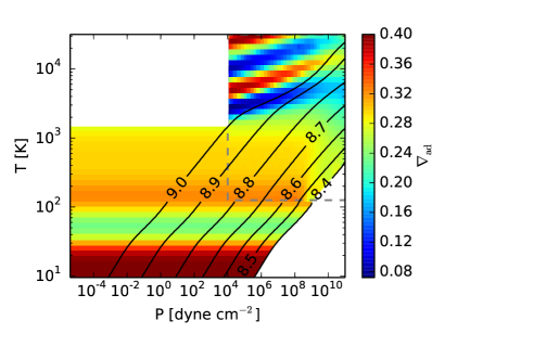
Figure 1.— Contour plot of the adiabatic gradient $\nabla_{\rm ad}$ for a hydrogen-helium mixture in thermodynamic equilibrium as a function of gas temperature and pressure. The upper-right rectangle encloses the region described by the original Saumon et al. (1995) EOS tables, while the rest of the plot is our extension. The black curves represent constant entropy adiabats, with the labels $\log_{10}(S)$ [erg K^-1 g^-1]. The regions in which the EOS is either invalid or not computed are masked in white. Further details about the masked regions can be found in Appendix A.1.

3.1. Intermediate $T$: Ideal Gas

For $300$ K $\lesssim T\lesssim 2000$ K, the hydrogen molecule is not energetic enough to dissociate and hydrogen behaves as an ideal diatomic gas with constant $\nabla_{\rm ad}$ (Figure 1). The monatomic helium component increases the adiabatic index slightly, so that $\nabla_{\rm ad}\approx 0.3$ rather than 2/7 for a pure diatomic gas.

3.2. High $T$: Dissociation and Ionization of Hydrogen

Hydrogen is molecular at low temperatures, dissociates at $T\gtrsim 2000-3000$ K, and ionizes at $T\gtrsim 10,000$ K. In stellar and giant planet interiors there is little overlap between the two processes: hydrogen is almost entirely dissociated into atoms by the time ionization becomes important.

As displayed in Figure 1, the adiabatic gradient decreases significantly in regions of partial dissociation and partial ionization. This reduction occurs because dissociation and ionization act as energy sinks. When internal energy is input into a partially dissociated gas, a portion is used to break down molecules, reducing the amount available to increase the temperature of the system.

An expression for $\nabla_{\rm ad}$ as a function of the dissociation fraction is presented in Appendix B.1. As expected, $\nabla_{\rm ad}$ is $2/7$ for pure molecular hydrogen and $2/5$ when hydrogen is fully dissociated, but decreases significantly during partial dissociation and is smallest when half of the gas is dissociated. Note that this behavior differs from a mixture of molecular and atomic hydrogen, for which $2/7<\nabla_{\rm ad}<2/5$.

3.3. Low $T$: Hydrogen Rotation and Spin Isomers

The (diatomic) hydrogen molecule has five degrees of freedom, three associated with translational motion and two associated with rotation. At $T$ well above the molecule’s excitation temperature for rotation, $\Theta_{r}\approx 85$ K (Kittel et al., 1981), its rotational states are fully excited and its EOS is that of an ideal diatomic gas (Section 3.1). As $T\rightarrow 0$, rotation ceases entirely and $\nabla_{\rm ad}\approx 2/5$, the value for an ideal monatomic gas. At temperatures comparable to $\Theta_{r}$, the rotational states of $H_{2}$ are are partially excited, and its EOS depends on the relative occupation of two isomeric forms, parahydrogen and orthohydrogen, distinguished by the spin symmetry of the molecule’s two protons.

Because protons are fermions, the Pauli exclusion principle implies that the total wave function of $H_{2}$ must be antisymmetric with respect to proton exchange. Two components of the wave function may provide this asymmetry—proton spins and the molecule’s rotational state. Parahydrogen has antiparallel proton spins and thus can only occupy symmetric rotational states with even angular quantum number $j$ (Farkas, 1935). In contrast, orthohydrogen has parallel proton spins, and can only occupy states with odd $j$. In thermal equilibrium at $T\rightarrow 0$ all hydrogen molecules are in the ground state with $j=0$, which corresponds to parahydrogen. As temperature increases, parahydrogen starts converting into orthohydrogen. Because the proton spin state is a triplet for orthohydrogen and a singlet for parahydrogen, this conversion plateaus at an ortho-para equilibrium ratio of 3:1 for $T\gtrsim 150$ K.

Spin conversion requires energy. In thermal equilibrium, a portion of any internal energy input at $20\lesssim T\lesssim 150$K is used to convert para- to orthohydrogen, reducing the amount available to increase $T$. As a result, $\nabla_{\rm ad}$ declines (Figure 1; see Appendix B.2 for further discussion).

3.3.1 Thermodynamic equilibrium of spin isomers

We conduct the majority of our calculations using the thermal equilibrium EOS illustrated in Figure 1. For reference, we also include results for a fixed 3:1 ortho-para ratio (used, e.g., by D’Angelo & Bodenheimer 2013).

Ortho- and parahydrogen remain in thermodynamic equilibrium if the isomers can interconvert on a timescale shorter than the atmosphere’s KH contraction time. In isolation, isomeric conversion requires a forbidden transition and has a timescale longer than the age of the universe (e.g., Pachucki & Komasa, 2008). Fast conversion requires a magnetic catalyst to aid the transition between the triplet and singlet spin states.

In astrophysical contexts, this catalyst is typically provided by collisions with ions such as $H^{+}$ or $H_{3}^{+}$ (e.g., Lique et al., 2012, 2014). At high densities, collisions with $H_{2}$ also contribute to conversion through interactions between the spin state and the magnetic dipole of the $H_{2}$ molecule (Huestis, 2008).

For a core of mass $M_{\rm crit}$, the KH contraction time during the slowest phase of growth is approximately the disk lifetime, $t_{\rm disk}\sim 3\times 10^{6}$ years. The thermodynamic equilibrium EOS is thus appropriate if the ortho-para equilibration time, $t_{\rm equil}$ is smaller than $t_{\rm disk}$. To determine whether this condition is met throughout the outer atmosphere (where $T\lesssim 150$ K), we check $t_{\rm equil}$ at the RCB and in the disk.

For core masses 6–30$M_{\oplus}$, our models produce RCB densities in the range $n=$1.5–5$\times 10^{14}$ during the longest phase of atmospheric evolution. The integrated column through the atmosphere at the RCB is $\sim$$10^{25}$cm^-2, larger than the $\sim$$10^{22}$–$10^{23}$ cm^-2 required to be optically thick to X-rays (Glassgold et al., 1997), so that ionizations in this interior portion of the atmosphere are attenuated. However, densities at the RCB are high enough that $H_{2}$ collisions cause substantial isomeric conversion. Extrapolating from calculations of catalysis by $O_{2}$, Conrath & Gierasch (1984) estimate a rate coefficient for conversion of $k_{H_{2}}=8\times 10^{-29}(T/125{\rm K})^{1/2}$ cm³ s^-1, marginally consistent with the production of non-equilibrium ortho-para ratios in solar system giants by upwellings and flows (e.g. Fouchet et al., 2003). Huestis (2008) estimates a faster rate coefficient given by $\log_{10}k_{H_{2}}[$cm³ s${}^{-1}]=10^{-28}[1.56+12.2\exp(-173{\rm K}/T)]$, consistent with laboratory experiments in liquid and gaseous $H_{2}$ (Farkas, 1935; Milenko et al., 1997). At $T=50$K ($T$ in the radiative region only varies from the disk temperature by an order unity factor; see Section 4.2), the equilibration time is

$$t_{\rm equil}=(k_{H_{2}}n_{H_{2}})^{-1}=\text{1.5--6}\times 10^{6}{\rm yr}\left(\frac{n}{10^{14}{\rm cm}^{-3}}\right)^{-1}\,\;,$$ (6)

which is comparable to or shorter than $t_{\rm disk}$.

Where the outer atmosphere matches conditions in the disk, we turn to calculations for protoplanetary disks for guidance. Boley et al. (2007) estimate a minimum $t_{\rm equil}\sim 300$ yr. Isomeric conversion primarily results from collisions between $H_{2}$ and ionic species, with $t_{\rm equil}\sim(k_{\rm ion}n_{\rm ion})^{-1}\sim 3\times 10^{6}$ yr $(n_{\rm ion}/10^{-4}{\rm cm}^{-3})^{-1}$, where $k_{\rm ion}\sim 10^{-10}$ cm³ s^-1 Walmsley et al. (2004). Typical ion abundances in disks are small, and calculations require involved photochemical networks. Detailed work suggests that ion densities of $10^{-4}$ cm^-3 are achieved beyond 30 AU and, depending on the disk’s dust complement, may be present throughout our region of interest (e.g., Glassgold et al., 1997; Bai & Goodman, 2009; Turner et al., 2010; Perez-Becker & Chiang, 2011). Inside $\sim$10AU, our atmospheric profiles are less sensitive to whether spin isomers reach thermodynamic equilibrium since disk temperatures exceed the peak conversion temperature of $\sim$50K.

We conclude that during the longest phase of atmospheric growth, to which $M_{\rm crit}$ is most sensitive, the equilibrium EOS is appropriate for the majority of and possibly all of our parameter space.

For our calculations, the difference between thermal equilibrium and a fixed ortho-para ratio of 3:1 is more prominent at larger stellocentric distances, where disk temperatures are lower. We find that a fixed ortho-para ratio may increase the atmospheric evolutionary time by up to a factor of $\sim$$3$ (corresponding to 100 AU in our fiducial disk; see Appendix B.2, Figure 15), and hence $M_{\rm crit}$ by up to a factor of 2. This effect is much smaller in the inner parts of the disk — the atmospheric growth time only increases by $\sim$$25$% at 10 AU.

4. Role of the Equation of State

Variations in the EOS, and hence $\nabla_{\rm ad}$, due to partial dissociation and fractional occupation of $\rm{H}_{2}$ rotational states affect atmospheric evolution by yielding: (1) a lower envelope luminosity $L$, and (2) a larger amount of radiated energy per unit of accreted mass $-dE/dM$, when compared to the polytropic EOS considered in Paper I. As a result, the rate of change in atmospheric mass,

$$\dot{M}=-\frac{L}{dE/dM},$$ (7)

(cf. Equation 5 and ignoring surface terms, which only become significant in the late stages of atmospheric evolution) is lower than in the polytropic case. Slower gas accretion increases the growth time of the atmosphere. Since envelope growth is faster for larger cores, we calculate a larger $M_{\rm crit}$.

Modifications in the EOS affect $L$ and $-dE/dM$ because both of these quantities depend on the global structure of the envelope. From Equation (3) applied at the RCB where $\nabla_{\rm ad}=\nabla_{\rm rad}$, and for a fixed atmospheric mass, the luminosity emerging from the convective interior scales as $L\propto T_{\rm RCB}^{4}/P_{\rm RCB}$. We have shown in Paper I that the outer radiative layer of the atmosphere is nearly isothermal, and that $T_{\rm RCB}$ is only a factor unity correction from the disk temperature, while the pressure in the radiative region increases exponentially with depth. It follows that $L$ primarily scales as $1/P_{\rm RCB}$. This pressure depth at the RCB depends on both the interior structure of the atmosphere at high temperatures, and on the matching to the nebula through the radiative region at low temperatures. Similarly, the EOS affects the distribution of total energy $E(r)$ throughout the envelope, and thus $-dE/dM$.

Since both dissociation deep in the convective interior and variable occupation of rotation states in the outer envelope affect atmospheric structure and evolution, it is helpful to separate these effects and study them independently.

Figure 2 shows the time evolution of atmospheres forming at 5 AU around cores of mass $M_{\rm c}=10M_{\oplus}$ and described by various equations of state, as follows:

1. Ideal gas polytrope with $\nabla_{\rm ad}=0.3$.

2. Ideal gas polytrope with $\nabla_{\rm ad}=0.3$ for $T>500$ K and realistic EOS for $T<500$ K, which includes the effects of fractional occupation of $\rm H_{2}$ rotational states.

3. Ideal gas polytrope with $\nabla_{\rm ad}=0.3$ for $T<500$ and realistic EOS for $T>500$ K , which includes the effects of hydrogen dissociation.

4. Realistic EOS at all $T$.

We choose $T=500$ K as the cutoff temperature because the hydrogen-helium mixture behaves like an ideal gas, with $\nabla_{\rm ad}=0.3$, in this temperature regime (see Figure 1). Both EOS 2 and EOS 3 yield slower gas accretion when compared to EOS 1. Noting the logarithmic scale in Figure 2, we see that the combined effect of fractional occupation of rotational states and dissociation is significantly greater than either individually. We explore these contributions in Sections 4.1 and 4.2.

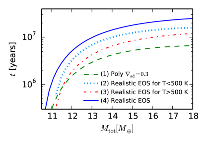
Figure 2.— Elapsed time to grow a planet of total mass (core + atmosphere) for a variety of EOS combinations (see text), for a planet forming at 5 AU and with a fixed core mass $M_{\rm c}=10M_{\oplus}$. Both hydrogen dissociation at high temperatures deep in the atmosphere and fractional occupation of $\rm H_{2}$ rotational states at low temperatures in the outer envelope result in slower gas accretion when compared to an ideal gas polytrope.

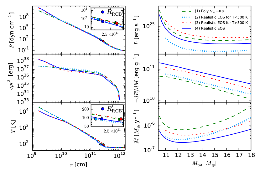
Figure 3.— We explore atmosphere growth around a core of $M_{\rm c}=10M_{\oplus}$ forming at 5 AU in our fiducial disk, for the EOS choices in Figure 2. Left panels show radial profiles of pressure (upper), $-e\rho r^{3}$ (middle) and temperature (lower), for a total mass (core + atmosphere) of $12M_{\oplus}$. Right panels display evolution with total mass of $L$ (upper), $-dE/dM$ (middle) and $\dot{M}$ (lower). Upper-left and upper-right: The variable occupation of $\rm H_{2}$ rotational states in the outer atmosphere results in a deeper RCB and a lower luminosity for the realistic EOS. Middle-left and middle-right: the (negative) total energy of the atmosphere is more concentrated at the bottom of the envelope when compared to an ideal gas polytrope due to $H_{2}$ dissociation. This increases the amount of energy per unit mass, $-dE/dM$, that needs to be radiated away to accrete the next parcel of gas. Lower-left: $H_{2}$ dissociation in the inner atmosphere decreases the temperature near the core. Lower-right: Dissociation and fractional occupation of rotational states reduce $\dot{M}$ and thus slow down atmospheric growth.

Throughout Section 4, we use a power-law opacity given by

$$\kappa=2F_{\kappa}\Big{(}\frac{T}{T_{\rm ref}}\Big{)}^{\beta},$$ (8)

with $\beta=2$, $F_{\kappa}=1$, and $T_{\rm{ref}}=100$K, appropriate for ice grains in the interstellar medium (ISM) (Bell & Lin, 1994). We improve our treatment of opacity in Section 5.

4.1. Role of $-dE/dM$

Variations in $\nabla_{\rm ad}$ due to dissociation increase $-dE/dM$ (Figure 3, middle-right). The atmosphere’s total (negative) energy at scale $r$, $-e\rho r^{3}$ is concentrated in the atmospheric interior for all EOSs (Figure 3, middle-left). However, $-e\rho r^{3}$ for EOS 3 and EOS 4 is much larger in magnitude near the core when compared to the others. This is due to the fact that $\nabla_{\rm ad}$ decreases in dissociation regions (Figure 1). Dissociation adds particles to the gas and hence increases its entropy. In order for entropy to stay constant with radius in the convective interior, the temperature must drop, lowering $\nabla_{\rm ad}$ and $|dT/dr|$ and resulting in lower temperatures near the core (cf. Figure 3, bottom-left). Because the specific internal energy $u\propto T$, dissociation decreases the total energy deep in the interior. Note that this loss of thermal energy due to dissociation can be large enough to trigger dynamical instabilities and eventual collapse in higher mass objects such as protostars (Larson, 1969) or during the runaway growth of giant planets (Bodenheimer et al., 1980).

The reduced total energy of an atmosphere with a realistic EOS can also be explained qualitatively using $\nabla_{\rm ad}$. The density profile in an adiabatic, non-self-gravitating atmosphere composed of an ideal gas scales as $\rho(r)\propto r^{-1/\nabla_{\rm ad}+1}$, and the total specific energy is $e(r)\propto 1/r$ (see Paper I). Thus $-e\rho r^{3}\sim r^{-1/\nabla_{\rm ad}+3}$. The total energy is concentrated near the core if $\nabla_{\rm ad}<1/3$, and at the outer boundary otherwise. Dissociation reduces $\nabla_{\rm ad}$, and for smaller $\nabla_{\rm ad}$, the total energy is more tightly packed in the envelope’s interior.

An atmosphere with more negative total energy (EOS 3 and 4) requires a larger amount of energy to be radiated away to bind the next batch of gas. This implies a larger $-dE/dM$ during atmospheric evolution (Figure 3, middle-right), and thus a lower $\dot{M}$ (Figure 3, lower-right).

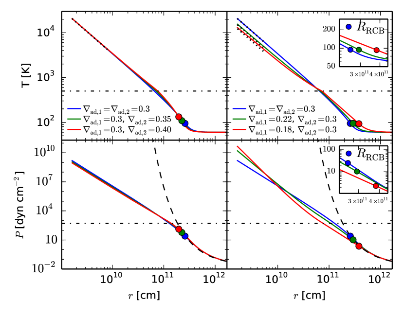
Figure 4.— As an illustrative numerical experiment, we explore atmosphere growth around a core with $M_{\rm c}=10M_{\oplus}$ forming at 5 AU, and with total mass (core + atmosphere) 12 $M_{\oplus}$, for the EOS choice of Equation (9) and various $\nabla_{\rm ad,1}$ and $\nabla_{\rm ad,2}$. In each panel, the circles mark the RCB location. The horizontal dash-dotted lines show the temperature $T_{\rm switch}=500$ K at which the adiabatic gradient changes. We show radial profiles of temperature (upper panels) and pressure (lower panels). Upper-left: fixed $\nabla_{\rm ad,1}$, varying $\nabla_{\rm ad,2}$. A larger $\nabla_{\rm ad,2}$ yields a deeper radiative region. Upper-right: varying $\nabla_{\rm ad,1}$, fixed $\nabla_{\rm ad,2}$. A lower $\nabla_{\rm ad,1}$ yields a more shallow radiative region. In both upper panels, the analytic profile of Equation (10) is over-plotted for comparison (dotted line) in regions of agreement. Lower-left: fixed $\nabla_{\rm ad,1}$, varying $\nabla_{\rm ad,2}$. Lower-right: varying $\nabla_{\rm ad,1}$, fixed $\nabla_{\rm ad,2}$. In both lower panels, the dashed black line is the analytic prediction for the pressure profile in the radiative zone, which agrees with the numerical results.

4.2. Role of $L$

The increase in $\nabla_{\rm ad}$ at low temperatures, where $H_{2}$ rotational states are not fully excited (Figure 3, upper-right) decreases the atmosphere’s luminosity. This result may be understood as consequence of matching between the atmosphere’s interior convective and exterior radiative profiles. The profiles must match at the RCB, constrained by the known total mass. This match determines the pressure at the RCB, $P_{\rm RCB}\propto\exp(R_{\rm B}/R_{\rm RCB})$. Higher $P_{\rm RCB}$ implies lower luminosity (Equation 3).

The adiabatic gradient of EOS 2 is larger, on average, than for EOS 1 in the outer part of the convective region. To understand how a variable, but overall larger $\nabla_{\rm ad}$ in the outer atmosphere affects evolution, we study the simplified problem of atmospheres composed of an ideal gas with adiabatic gradient

$$\nabla_{\rm ad}=\left\{\begin{array}[]{l l}\nabla_{\rm ad,1},&\quad T>500\text{ K}\\ \nabla_{\rm ad,2},&\quad T<500\text{ K}\end{array}\right.$$ (9)

where $\nabla_{\rm ad,1}$ and $\nabla_{\rm ad,2}$ are constant (Figure 4).

The adiabatic gradient $\nabla_{\rm ad,1}$ dictates the temperature profile deep in the convective interior. Deep in the atmosphere, where $r\ll R_{\rm RCB}$, virial equilibrium yields a temperature profile

$$T(r)\approx\frac{\nabla_{\rm ad,1}GM_{\rm c}}{\mathcal{R}r}.$$ (10)

Even though $\nabla_{\rm ad,1}$ is an order unity coefficient, the temperature scaling with $\nabla_{\rm ad,1}$ in Equation (10) is exact (Figure 4, upper-right panel). Because the radial temperature profile in the atmospheric interior is set by $\nabla_{\rm ad,1}$, the radius $R_{\rm switch}$ at which the adiabatic gradient changes shows little variation with $\nabla_{\rm ad,2}$.

The RCB temperature, $T_{\rm RCB}$, is an order unity correction from the disk temperature that depends on the adiabatic gradient in the outer envelope, $\nabla_{\rm ad,2}$. We have shown in Paper I that $T_{\rm RCB}\simeq T_{\rm d}(1-2\nabla_{\rm ad,2})^{-1/2}$ (for $\beta=2$ in Equation 8). This approximation agrees with the numerically calculated $T_{\rm RCB}$ shown in Figure 4 to within 5%. Note that $T_{\rm RCB}$ modestly increases with $\nabla_{\rm ad,2}$ (upper-left panel), and is constant for fixed $\nabla_{\rm ad,2}$ regardless of $\nabla_{\rm ad,1}$ (upper-right panel).

When these temperature conditions are matched for a fixed atmosphere mass, Figure 4 shows that a larger adiabatic gradient in the outer atmosphere results in a deeper radiative region. We can understand this effect by assuming that $R_{\rm switch}$ is fixed. A steeper adiabat (i.e., with a larger adiabatic gradient) that starts at a given depth (here $R_{\rm switch}$) will match the fixed RCB temperature at a smaller radius. A quantitative scaling of $R_{\rm RCB}$ is not possible because Equation (10) is only valid to order of magnitude at $R_{\rm switch}$ and relatively small variations in the physical depth of the RCB can impact the RCB pressure significantly. It follows that $L\propto 1/P_{\rm RCB}$ decreases with increasing outer $\nabla_{\rm ad}$; thus the overall larger adiabatic gradient due to the variable occupation of rotation states at low temperatures decreases $L$ and slows down growth.

5. Impact of Opacity on Atmosphere Evolution

Our calculations so far have assumed that the dust opacity in the radiative region of the atmosphere is given by the standard ISM opacity. However, our scenario of low planetesimal accretion is likely to favor lower dust opacities, due to grain growth and dust settling. Grain growth, in particular, lowers the absolute value of the opacity, and may change the particle size distribution when compared to the standard ISM size distribution (e.g., Pollack et al. 1985). Enhanced metallicity due to planetesimal accretion, by construction not present during our atmosphere’s growth, cannot make up for this reduction.

Although grain growth and evidence for a non-ISM size distribution have been observed in protoplanetary disks (e.g., Beckwith et al. 1990, Beckwith & Sargent 1991, Pérez et al. 2012), the size distribution of dust particles has not been tightly constrained. Typically, the differential grain size distribution is assumed to be a power-law:

$$\frac{dN}{ds}\propto s^{-p},$$ (11)

where $dN$ is the number of particles with sizes between $s$ and $s+ds$ and $p=3.5$ (a standard Dohnanyi 1969 collisional cascade; appropriate for the ISM) or $p=2.5$ (an approximation for coagulation). In this work we use the D’Alessio et al. (2001) frequency-dependent opacity tables to obtain the temperature-dependent Rosseland mean opacity $\kappa$. We take as a fiducial case a maximum particle size $s_{\rm max}=1$ cm and a grain size distribution given by Equation (11) with $p=3.5$. Other choices for the power-law coefficient $p$ are discussed later in this section. Though we choose our opacities to reflect ambient conditions in the disk, we note that grains can also grow within an accreting atmosphere, decreasing its opacity at depth (Movshovitz et al., 2010; Mordasini, 2014; Ormel, 2014).

The D’Alessio et al. (2001) opacities are only relevant at temperatures that are sufficiently low for dust grains to remain solid ($T\lesssim 1000$ K). At higher temperatures, we use the Bell & Lin (1994) analytic opacity laws, ensuring smooth transition from the grain growth opacities, as illustrated in Figure 16.

The sharp drop in opacity ($\kappa\sim T^{-24}$, see Figure 17) due to dust sublimation lowers the radiative temperature gradient significantly (see Equation 3), and may thus generate radiative layers within the inner region of the atmosphere (see Appendix C, Figure 17). Additionally, the weak temperature dependence of grain growth opacities may cause larger outer radiative zones than when ISM opacities are used. This could pose two challenges for our model:

1. The additional luminosity, $\Delta L$, generated in the outer radiative layer of the envelope may not satisfy $\Delta L\ll L$, where $L$ is the assumed fixed atmospheric luminosity. For $p=3.5$ in Equation (11), we have checked that $\Delta L\ll L$ in all the cases presented in this study. For $p=2.5$, however, this approximation breaks down at low core masses, as we show in §6.

2. As little as half of the atmosphere’s luminosity is generated in the innermost convective layer when radiative windows exist. We must therefore check that our assumption of constant $L$ does not substantially change the structure of the atmosphere in the region of the radiative windows. Fortunately, these radiative windows are either very narrow compared to the height of the convective regions (Figure 17, middle panel), or have $\nabla_{\rm ad}\approx\nabla_{\rm rad}$ throughout, which makes the distinction between convective and radiative layers less pronounced (Figure 17, bottom panel). This implies that the entropy drop across the radiative windows is small. We investigate the luminosity structure in greater detail in Appendix C and conclude that our model remains a reasonably good approximation even in the presence of radiative windows.

We thus find that our atmospheric and cooling model is valid in our regions of interest, with some exceptions discussed in §6.

6. Critical Core Mass

In this section we put together the results obtained in Sections §4 and §5, and determine the minimum core mass, $M_{\rm crit}$, to initiate runaway gas accretion during a typical protoplanetary disk lifetime, $t=3$ Myr. As in Paper I, we quantify the runaway accretion time $t_{\rm run}$ as the time at which the atmosphere growth timescale $M_{\rm atm}/\dot{M}$ drops to 10% of its maximum value (see Paper I for details).

Figure 5 displays the time evolution and the runaway growth time for atmospheres forming around cores with masses between 15 $M_{\oplus}$ and 25 $M_{\oplus}$ at $a=10$ AU in our fiducial disk, for a realistic EOS with an equilibrium ortho-to-para ratio and standard ISM opacity. Higher mass cores have shorter $t_{\rm run}$, consistent with the results of Paper I. We also note that $M_{\rm atm}$ at $t_{\rm run}$ is larger for the realistic EOS than for the polytropic EOS considered in Paper I, for the same core mass.

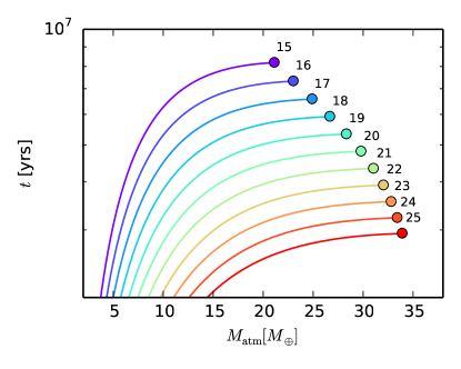
Figure 5.— Elapsed time as a function of atmosphere mass, for cores with fixed masses between $15M_{\oplus}$ and $25M_{\oplus}$ at $a=10$ AU in our fiducial disk, for a realistic EOS with an equilibrium ortho-to-para ratio and standard ISM opacity. The circles mark the runaway growth time. The numbers label the core mass in Earth masses. A larger core mass results in a lower $t_{\rm run}$.

Figure 6, upper panel, displays $M_{\rm crit}$ for a gas described by a realistic EOS and an ISM dust opacity. The results of Paper I for an ideal diatomic gas are plotted for comparison. When compared to an ideal gas polytrope, the inclusion of realistic EOS effects increases $M_{\rm crit}$ by a factor of $\sim$2 if the $H_{2}$ spin isomers are in equilibrium, and by a factor of $\sim$$2-4$ for a fixed 3:1 ortho-to-para ratio. This latter increase is more significant at larger stellocentric distances. In Figure 6, bottom panel, we compare our results with those for a disk with a gas surface density an order of magnitude larger than $\Sigma_{\rm d}$ of our fiducial disk (see Equation 1), and find that $M_{\rm crit}$ reduces by $\sim$15-25$\%$.

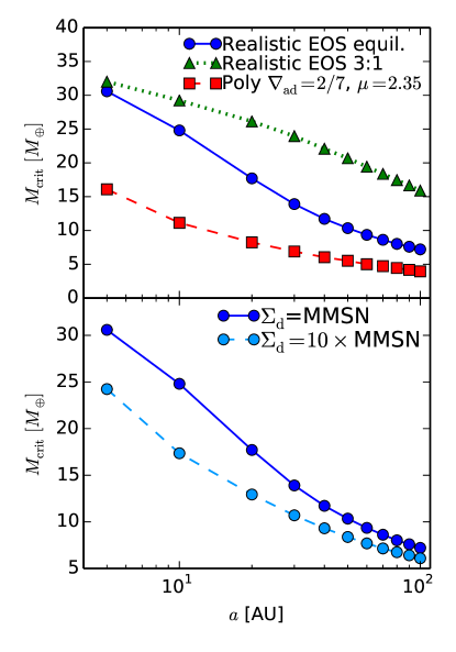
Figure 6.— Top panel: The minimum core mass for an atmosphere to initiate runaway gas accretion within the lifetime of a typical protoplanetary disk $t\sim 3$ Myrs as a function of semimajor axis, for a realistic hydrogen-helium mixture and a standard ISM opacity. The results of Paper I for an ideal diatomic gas are plotted for comparison. The realistic EOS yields core masses larger by a factor of $\sim$2 when compared to the polytrope, for an equilibrium ortho-to-para ratio. The critical core mass is $\sim$$2-4$ times larger than the polytrope case for a fixed 3:1 ratio between the $H_{2}$ spin isomers. The increase is more pronounced at larger stellocentric distances. Bottom panel: Critical core mass as a function of semimajor axis for a disk gas surface density 10 times larger than that of our fiducial disk. A larger $\Sigma_{\rm d}$ reduces $M_{\rm crit}$ by $\sim$$15-25\%$.

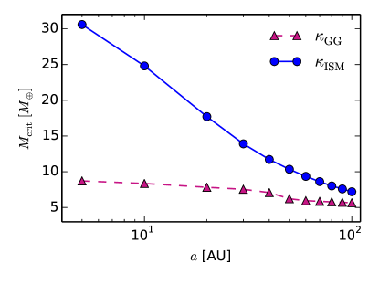
Figure 7.— Critical core mass as a function of semimajor axis for a realistic EOS with an equilibrium ortho-to-para ratio and radiative opacities that account for grain growth (purple triangles, with $p=3.5$ and $a_{\rm max}=1$ cm; see text for details). The critical core mass is lower than it would be if dust grains had an ISM-like size distribution (blue circles).

Figure 7 shows $M_{\rm crit}$ as a function of semimajor axis, for a realistic EOS with an equilibrium ortho-to-para ratio and grain growth opacity with a size distribution given by Equation (11) with $p=3.5$ and maximum particle size $s_{\rm max}=1$ cm. The critical core mass is lower than in the standard interstellar opacity case, and less sensitive to location in the disk. Location primarily affects the atmosphere through the opacity in the outer envelope, which depends on disk temperature. For the simplified analytic model developed in Paper I, we approximated $t_{\rm run}$ by $t_{\rm co}$, the time when $M_{\rm atm}=M_{\rm c}$, and found that $t_{\rm co}\sim T_{\rm d}^{\beta+1/2}$, with $\beta$ the power-law exponent in Equation (8). Opacity is less sensitive to temperature variations for larger grains and has an almost flat profile (see Figure 16), which results in $\beta\ll 1$ and a much weaker temperature (and therefore semimajor axis) dependence of $M_{\rm crit}$, as seen in Figure 7. Moreover, grain growth reduces the absolute value of the opacity, which also lowers $M_{\rm crit}$.

Figure 8.— Runaway accretion times for a realistic EOS with an equilibrium ortho-to-para ratio and different grain size distributions, for an atmosphere forming around a core with $M_{\rm c}=4M_{\oplus}$. The lines marked by purple and orange triangles have grain growth opacities with $a_{\rm max}=1$ cm, and $p=3.5$ and $p=2.5$, respectively (see text for details). The blue circle line has an ISM power-law opacity. The runaway accretion time is more than one order of magnitude lower when coagulation is accounted for, i.e. $p=2.5$.

In Equation (11), the coefficient $p=3.5$ corresponds to a standard collisional cascade. If coagulation is taken into account, the exponent $p$ can be approximated as $p=2.5$ (D’Alessio et al., 2001). This results in a flatter and significantly lower opacity (see Appendix C), which may substantially reduce $M_{\rm crit}$. However, we have found that our model breaks down for low core masses ($M_{\rm c}\lesssim 3M_{\oplus}$) under our assumption of constant luminosity in the outer radiative layer. Figure 8 shows the runaway accretion time $t_{\rm run}$ as a function of semimajor axis for the lowest core mass for which our model is valid, $M_{\rm c}=4M_{\oplus}$. The runaway accretion time is more than one order of magnitude lower for $p=2.5$, which implies that $M_{\rm crit}$ may be, in fact, significantly lower than presented in Figure 7. In other words, grain growth can yield critical core masses up to an order of magnitude lower than in the case where interstellar opacities are used.

In summary, we have found $M_{\rm crit}\sim 30M_{\oplus}$ at 5 AU, steadily decreasing to $\sim$$7M_{\oplus}$ at 100 AU, for a realistic EOS with the $H_{2}$ spin isomers in equilibrium and interstellar opacity. For a fixed 3:1 ortho-to-para ratio and interstellar opacity, $M_{\rm crit}$ is $\sim$$32M_{\oplus}$ at 5 AU and decreases to $\sim$$15M_{\oplus}$ at 100 AU. For a grain growth opacity with a size distribution given by Equation (11) with $p=3.5$ and an equilibrium ortho-to-para ratio, $M_{\rm crit}$ significantly drops to $\sim$$8M_{\oplus}$ at 5 AU and $\sim$$5M_{\oplus}$ at 100 AU. Accounting for coagulation (i.e., $p=2.5$) $M_{\rm crit}$ is less than $4M_{\oplus}$ and may be up to an order of magnitude smaller.

7. Effects of Planetesimal Accretion

This study considers protoplanets with fully formed cores for which planetesimal accretion is negligible and KH contraction dominates the luminosity evolution of the atmosphere. This approach contrasts with that of models which assume high planetesimal accretion rates and find that the atmosphere is in steady state and solely heated due to accretion of solids. In both cases, as the envelope and core become comparable in mass, hydrostatic balance no longer holds and runaway gas accretion commences. For fast accretion, $M_{\rm crit}$ is uniquely defined as the maximum core mass for which the atmosphere is still in hydrostatic equilibrium for a fixed planetesimal accretion rate and a set of disk conditions. In this section we compare our results for $M_{\rm crit}$ to analogous results from steady-state fast planetesimal accretion calculations. We discuss the core accretion rates that are necessary for our regime to be valid in §7.1. In §7.2, we estimate core growth at the maximum rate for which the KH regime is valid, and show it is negligible over the timescale on which the atmosphere evolves. Finally, we compare our results with those assuming fast planetesimal accretion in §7.3.

7.1. Planetesimal Accretion Rates

Kelvin-Helmholtz contraction dominates an atmosphere’s luminosity if $L_{\mathrm{acc}}<L_{\rm{KH}}$, where $L_{\rm{acc}}$ is the accretion luminosity,

$$L_{acc}=G\frac{M_{\rm{c}}\dot{M_{\rm{c}}}}{R_{\rm{c}}},$$ (12)

and $L_{\rm KH}$ is given by Equation (5) with $L_{\rm c}=\Gamma=0$. This condition is satisfied as long as the planetesimal accretion rate

$$\dot{M_{\rm c}}<\dot{M}_{\rm c,KH}\equiv\frac{L_{\rm KH}R_{\rm c}}{GM_{\rm c}}.$$ (13)

To illustrate the magnitude of $\dot{M}_{\rm c,KH}$, we choose as a fiducial case an atmosphere forming at 30 AU and with a core mass of $10M_{\oplus}$. Since analytic studies of critical core masses at high planetesimal accretion rates assume an ideal gas EOS, for ease of comparison we choose an ideal gas polytropic EOS with constant adiabatic gradient $\nabla_{\rm ad}=2/7$ and mean molecular weight $\mu=2.35$ (see also Paper I). For this choice of parameters, the runaway accretion time is $t_{\rm run}\sim$ 1.4 Myrs, which is within the typical lifetime of a protoplanetary disk. We also estimate two reference accretion rates. The first one is the core accretion rate $\dot{M}_{\rm c,acc}$ needed to grow the core to $M_{\rm c}=10M_{\oplus}$ on the same timescale as our model atmosphere, $\tau=1.4$ Myrs:

$$\dot{M}_{\rm{c,acc}}(M_{\rm{c}})\sim\frac{M_{\rm{c}}}{\tau}.$$ (14)

The second reference planetesimal accretion rate is $\dot{M}_{\rm c,Hill}$, a typically assumed planetesimal accretion rate for which the random velocities of the planetesimals are of the order of the Hill velocity around the protoplanetary core (for a review, see Goldreich et al. 2004). Following R06 (equation A1),

$$\dot{M}_{\rm{c,Hill}}=\Omega\Sigma_{\rm p}R_{\rm c}R_{\rm H},$$ (15)

where $\Sigma_{\rm p}$ is the surface density of solids, assumed to satisfy $\Sigma_{\rm d}\approx 100\Sigma_{\rm p}$ for a dust-to-gas ratio of 0.01.

Figure 9 shows that $\dot{M}_{\rm c,KH}$ is $\sim 2-3$ orders of magnitude lower than $\dot{M}_{\rm c,acc}$. Had the core accreted planetesimals at the $\dot{M}_{\rm c,KH}$ rate since it started forming, it could not have grown large enough to attract an atmosphere within a typical disk lifetime. Our model requires that the planetesimal accretion rate is initially large during core growth, then significantly reduces as the gaseous envelope accumulates, as suggested by, e.g., Pollack et al. (1996). This is a plausible scenario: the core’s feeding zone may be depleted of solids if it is not refilled by radial drift of planetesimals through the nebula, or the core may form in the inner part of the disk and later be scattered outwards by other giants in the system (Ida et al., 2013).

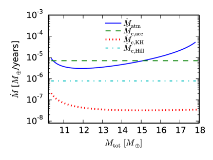
Figure 9.— Various accretion rates for a planet forming at 30 AU and with a core mass $M_{\rm c}=10M_{\oplus}$, using a polyropic EOS and ISM power-law opacity. For this choice of parameters, the runaway accretion time is $t_{\rm run}\sim 1.4$ Myrs. The $\dot{M}_{\rm{atm}}$ (solid blue) curve represents the growth rate of the atmosphere as estimated by our model. The core accretion rate $\dot{M}_{\rm c,acc}$ (dashed green) necessary to grow the core on the timescale $t_{\rm run}$ is larger than $\dot{M}_{\rm c,KH}$ (dotted red), the maximum planetesimal accretion rate during KH contraction for which our regime is valid (see text). The frequently used planetesimal accretion rate $\dot{M}_{\rm c,Hill}$ (dashed-dotted light blue) for which the random velocity of the planetesimals is given by the Hill velocity due to the core (see text), also exceeds $\dot{M}_{\rm c,KH}$.This motivates our requirement that planetesimal accretion must have slowed down after core growth for our model to be valid.

7.2. Core Growth during KH Contraction

Planetesimal accretion during the KH contraction phase of atmosphere growth at a rate $\dot{M}_{\rm c}<\dot{M}_{\rm{c,KH}}$ cannot alter the core mass enough to affect the time evolution of the atmosphere. We can quantitatively estimate the maximum increase in core mass as

$$\Delta M_{\rm{c}}=\int_{0}^{t_{\rm{run}}}\dot{M_{\rm{c}}}dt\approx\sum_{i}\dot{M_{\rm{c}}}_{i}\Delta t_{i},$$ (16)

where the accretion rate $\dot{M_{\rm{c}}}_{i}$ is given by

$$\dot{M_{\rm{c}}}_{i}=\frac{L_{i}R_{\rm c}}{GM_{\rm{c}}}$$ (17)

from Equation (12), with $L_{i}$ the luminosity of the atmosphere at time $t_{i}$ in our model. For $M_{\rm{c}}=10M_{\oplus}$, we find $\Delta M_{\rm{c}}\approx 0.05M_{\oplus}\ll 10M_{\oplus}$. Core growth is negligible in our regime, and the time evolution of the atmosphere is thus insensitive to core mass changes at a rate imposed by the assumption that $L_{\rm{acc}}<L_{\rm{KH}}$.

7.3. Comparison with Steady-State Results

We compare our results for $M_{\rm crit}$ with those of studies that assume large planetesimal accretion rates. In principle, the disk lifetime could be short enough that our calculated $M_{\rm crit}$ could exceed the $M_{\rm crit}$ estimated for a steady-state, accretion-heated core. This prospect is not self-contradictory since at higher luminosity, an atmosphere evolves more quickly and hence reaches steady state on a timescale shorter than our calculated KH contraction time. We show here that disk lifetimes are long enough that this is not the case. Our model yields lower core masses than those found when fast planetesimal accretion is considered.

The critical core mass is larger for higher planetesimal accretion, as additional heating increases the core mass required for collapse. As such, if atmosphere collapse does not occur for the lowest value of $\dot{M}_{\rm c,KH}$ over the course of the atmosphere’s growth, then it can only occur in the KH dominated regime.

In order to estimate the critical core mass $M_{\rm crit,KH}$ corresponding to planetesimal accretion at the rate $\dot{M}_{\rm c,KH}$, we use the results of R06 for low luminosity atmospheres forming in the outer disk ($\gtrsim 2-5$ AU). R06 assumes an ideal gas polytropic EOS and an opacity lower than that of the ISM (see Equation 8). For comparison, we calculate $M_{\rm crit}$ for an ideal gas polytrope and an opacity, $\kappa$, given by Equation 8 with $F_{\kappa}$ reduced by a factor of 100. This choice is comparable to the opacity law used by R06.

Following R06, we find that the critical core mass when accretion luminosity dominates the evolution of the atmosphere can be expressed as

$$M_{\rm{crit,KH}}\sim\Big{[}\frac{\min[\dot{M}_{\rm c,KH}(M_{\rm{c}})]}{64\pi^{2}C}\frac{\kappa}{\sigma G^{3}}\frac{1}{R_{\rm c}M_{\rm c}^{1/3}}\Big{(}\frac{k_{B}}{\mu m_{p}}\Big{)}^{4}\Big{]}^{3/5},$$ (18)

where $C$ is an order unity constant depending on the adiabatic gradient and disk properties (see R06, Equation B3). From Equation (13), the accretion rate $\dot{M}_{\rm c,KH}$ depends on the core mass $M_{\rm c}$. We find $M_{\rm crit,KH}$ numerically by setting $M_{\rm c}=M_{\rm crit,KH}$ on the right-hand side of Equation (18). The result is displayed in Figure 10; the critical core mass corresponding to planetesimal accretion at the rates displayed in Figure 9 is displayed for comparison.

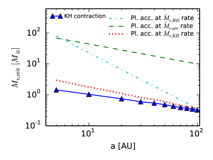
Figure 10.— Comparison between the critical core mass $M_{\rm{crit,KH}}$ given significant planetesimal accretion and the critical core mass when gas contraction dominates, for a polytropic EOS and an ISM opacity reduced by a factor of 100. Our results yield lower core masses than in the fast planetesimal accretion case (e.g., Rafikov 2006). The critical core mass corresponding to $\dot{M}_{\rm c,Hill}$ and $\dot{M}_{\rm c,acc}$ from Figure 9 is plotted for comparison.

The critical core mass in the regime where KH contraction dominates is smaller than in the case in which planetesimal accretion dominates the evolution of the atmosphere. This leads to two conclusions:

1. Planetesimal accretion can be safely ignored in our regime.

2. Giant planets can form from smaller cores if planetesimal accretion significantly reduces during atmosphere growth.

8. Summary

In this paper we study the formation of giant planets embedded in a gas disk. We consider atmospheric evolution around fully grown cores and determine the minimum (critical) core mass, $M_{\rm crit}$, required to form a gas giant during the typical lifetime of a protoplanetary disk. We improve the model developed in Piso & Youdin (2014, hereafter Paper I) by including realistic equation of state (EOS) tables and dust opacities.

For a realistic EOS with the molecular hydrogen ($H_{2}$) spin isomers in thermal equilibrium, and grain growth opacity with maximum particle size $s_{\rm max}=1$ cm and a power-law size distribution (11) with $p=3.5$, $M_{\rm crit}$ is $\sim$$8M_{\oplus}$ at 5 AU in our fiducial disk and drops to $\sim$$5M_{\oplus}$ at 100 AU. The realistic EOS and grain growth opacity have two competing effects on $M_{\rm crit}$:

1. Realistic EOS effects increase $M_{\rm crit}$ by a factor of $\sim$$2$ when compared to the ideal gas polytrope, for an equilibrium ratio of ortho- and parahydrogen. If the $H_{2}$ spin isomers are in a fixed 3:1 ratio, $M_{\rm crit}$ increases by a factor of $\sim$$2-4$ when compared to the polytrope. This increase is most significant at larger stellocentric distances, where disk temperatures are lower than the peak ortho-to-para conversion temperature of $\sim$$50$ K.

2. Grain growth opacities decrease $M_{\rm crit}$ by a factor of $\sim$$3.5$ at 5 AU and by a factor of $\sim$$1.2$ at 100 AU, when compared to ISM opacities, for a particle distribution given by the power-law (11) with $p=3.5$ and a maximum particle size of 1 cm. The critical core mass is less sensitive to the location in the disk when realistic opacities are used. If $p=2.5$, an approximation for coagulation, $M_{\rm crit}$ further reduces by up to an order of magnitude.

In our core accretion models, the dissociation of molecular hydrogen slows the atmospheric cooling and gas accretion rate. This finding is somewhat surprising because $H_{2}$ dissociation can trigger the gravitational collapse of protostellar or planetary mass gas clouds (Bodenheimer et al. 1980, Inutsuka 2012). The presence of a massive solid core is the key factor that prevents dissociation from inducing a global collapse in our models.

Our results yield lower core masses than analogous results that consider high planetesimal accretion rates for which the core and atmosphere grow simultaneously. It is thus possible to form a giant planet from a smaller core if the core grows first, then the accretion rate of solids is reduced and a gaseous envelope is accumulated. Moreover, since additional heat sources such as planetesimal accretion limit the ability of the atmosphere to cool and undergo Kelvin-Helmholtz contraction, our results represent a true minimum on the core mass needed to form a giant planet during the typical lifetime of a protoplanetary disk.

Appendix A Equation of State Table Extension

In this study we consider atmosphere growth in the outer parts of protoplanetary disks ($5<a<100$ AU), where temperature and pressure drop to as little as $T\sim 20$ K and $P\sim 4\times 10^{-6}$ dyn cm^-2 for our fiducial disk model (see equations 1 and 1). We model the nebular gas using the EOS tables of Saumon et al. (1995). However, these tables only cover the relatively high temperature and pressure ranges $2.1<\log_{10}T(\rm{K})<7.06$ and $4.0<\log_{10}P$(dyn cm${}^{-2})<19.0$. We thus need to extend the tables to lower $T$ and $P$. We calculate $\nabla_{\rm ad}$ for

$$1.0 < \log_{10}T<2.1$$ (A1)

$$-5.4 < \log_{10}P<4.0$$ (A2)

using the following method.

A.1. Hydrogen

Following Kittel et al. (1981), we calculate $\nabla_{\rm ad}$ from the partition function for the internal energy of a system of hydrogen gas molecules (see also D’Angelo & Bodenheimer 2013 for EOS calculations that take into account hydrogen isomers). We begin by writing the partition function $Z$ of a gas molecule of mass $m$ as the product of the partition functions associated with each type of internal energy:

$$Z=Z_{t}Z_{r}Z_{v}\;\;,$$ (A3)

where $Z_{t}$, $Z_{r}$, $Z_{v}$ are associated with translation, rotation, and vibration, respectively.

In the classical limit, the molecule’s center of mass motion generates

$$Z_{t}=(mk_{B}T/2\pi\hbar^{2})^{3/2}V,$$ (A4)

where $T$ and $V$ are the gas temperature and volume, respectively, and $\hbar$ is the reduced Planck constant. The rotational partition function is

$$Z_{r}=\sum_{j=0}^{\infty}(2j+1)\exp{\Big{[}\frac{-j(j+1)\Theta_{r}}{T}\Big{]}},$$ (A5)

where the characteristic temperature for rotational motion $\Theta_{r}\approx 85$ K for hydrogen. However, molecular hydrogen occurs in two isomeric forms: parahydrogen with a symmetric (even) rotational wavefunction, and orthohydrogen with an antisymmetric (odd) wavefunction (see Section 3). The rotational partition functions for ortho- and parahydrogen are thus

$$Z_{\rm{r,para}}=\sum_{j=0}^{\infty}\frac{1+(-1)^{j}}{2}(2j+1)\exp\Big{[}-\frac{j(j+1)\Theta_{r}}{T}\Big{]}$$ (A6)

and

$$Z_{\rm{r,ortho}}=3\sum_{j=0}^{\infty}\frac{1-(-1)^{j}}{2}(2j+1)\exp\Big{[}-\frac{j(j+1)\Theta_{r}}{T}\Big{]}\;\;.$$ (A7)

The factor of 3 in Equation (A7) accounts for the three-fold degeneracy of the ortho state.

In thermal equilibrium, the spin isomers have a combined partition function $Z_{\rm r}=Z_{\rm{r,ortho}}+Z_{\rm{r,para}}$, which can be written

$$Z_{r}=\sum_{j=0}^{\infty}(2-(-1)^{j})(2j+1)\exp{\Big{[}\frac{-j(j+1)\Theta_{r}}{T}\Big{]}}\;\;.$$ (A8)

For a fixed 3:1 ortho-to-para ratio, the combined partition function is $Z_{\rm r}=Z_{\rm r,para}^{1/4}Z_{\rm r,ortho}^{3/4}$. In our range of temperatures of interest, we find that $Z_{r}$ converges after about 25 terms in the series, for both the equilibrium and 3:1 cases.

Note that $Z_{\rm r,ortho}\rightarrow 0$ and $Z_{\rm r,para}\rightarrow 1$ as $T\rightarrow 0$. This is inconsistent with a fixed 3:1 ortho-to-para ratio, since $Z_{\rm r,ortho}\rightarrow 0$ implies that there is no orthohydrogen in the system. Boley et al. (2007) and D’Angelo & Bodenheimer (2013) ensure that this requirement is not violated by using a normalized orthohydrogen partition function, $Z^{\prime}_{\rm r,ortho}=Z_{\rm r,ortho}\exp(2\theta_{\rm r}/T)$, which reduces the energy of the lowest rotational state for orthohydrogen from $2k_{\rm B}\theta_{\rm r}$ per molecule to zero. This decreases the total internal energy of the system by a constant factor, but does not change $c_{\rm v}$, $\nabla_{\rm ad}$, or the relative internal energies of static atmospheric profiles, and therefore does not affect atmospheric evolution.

Finally, the partition function for vibrational motion is given by:

$$Z_{v}=[1-\exp{(\theta_{v}/T)}]^{-1},$$ (A9)

where the characteristic temperature for vibrational motion is $\theta_{v}\approx 6140$ K for hydrogen.

For a system of $N$ particles of mass $m$, the partition function of the ensemble is $Z_{\rm N}=(1/N!)Z^{N}$. Given $Z_{\rm N}$ as a function of $(V,T)$, the internal energy per mass, entropy per mass and specific heat capacity can be written as

$$u=\mathcal{R}T^{2}\Big{(}\frac{\partial\ln{Z}}{\partial T}\Big{)}_{V}$$ (A10)

$$S=\mathcal{R}\ln{Z}+\frac{u}{T}-\frac{\mathcal{R}}{N}\ln N!$$ (A11)

$$c_{\rm V}=\Big{(}\frac{\partial u}{\partial T}\Big{)}_{V}.$$ (A12)

Note that, following the convention of Saumon et al. (1995), we use $S$ to denote entropy per mass ($[S]=$erg K^-1 g^-1). Since $Z=Z_{t}Z_{r}Z_{v}$, we may write $u=u_{t}+u_{r}+u_{v}$ and $S=S_{t}+S_{r}+S_{v}$, where variables subscripted $t$, $r$, and $v$ are the quantities corresponding to the individual translation, rotation and vibration partition functions, respectively. We include the term $\mathcal{R}/N\ln N!$ from Equation (A11) in $S_{\rm t}$.

In the temperature regime for which the rotational states of $\rm{H}_{2}$ are selectively occupied, the total number of particles in the system is constant and we may use the ideal gas law, $P=\rho\mathcal{R}T$. With Equations (A10), (A11), and Stirling’s approximation, $\ln N!\approx N\ln N-N$, the resulting entropy per mass due to translational motion is

$$S_{\rm t}=\mathcal{R}\Big{[}\frac{5}{2}\ln{T}-\ln{P}+\ln\Big{(}\frac{(2\pi)^{3/2}\mathcal{R}^{5/2}m^{4}}{h^{3}}\Big{)}+\frac{5}{2}\Big{]}$$ (A13)

Equation (A13) is known as the Sackur-Tetrode formula.

The internal energy per mass due to translational motion is given by:

$$u_{t}=\frac{3}{2}\mathcal{R}T$$ (A14)

Putting all of the above together, we can now evaluate the thermodynamic quantities needed to extend the Saumon et al. (1995) EOS tables to low temperatures and pressures.

1. Density. In the low temperature, low pressure regime, $\rho$ is related to $T$ and $P$ by the ideal gas law.

2. Internal energy per mass. $u=u_{t}+u_{r}+u_{v}$, where $u_{t}$ is given by Equation (A14), and $u_{r}$ and $u_{v}$ are determined using Equations (A8), (A9) and (A10) above.

3. Entropy per unit mass. Similarly, $S=S_{t}+S_{r}+S_{v}$, where $S_{t}$ is given by Equation (A13), and $S_{r}$ and $S_{v}$ can be determined from Equation (A11) and the calculated expressions for $u_{r}$ and $u_{v}$, respectively.

4. Entropy logarithmic derivatives. The logarithmic derivatives $S_{T}$ and $S_{P}$ are given by:

   $$S_{T}=\frac{\partial\ln{S}}{\partial\ln{T}}\Big{|}_{P}$$ (A15)

   and

   $$S_{P}=\frac{\partial\ln{S}}{\partial\ln{P}}\Big{|}_{T}$$ (A16)

   We calculate $S_{T}$ and $S_{P}$ through finite differencing.

5. Adiabatic gradient $\nabla_{\rm ad}$. The adiabatic gradient is defined as:

   $$\nabla_{\rm ad}=\frac{\partial\ln{T}}{\partial\ln{P}}\Big{|}_{S}=-\frac{S_{P}}{S_{T}}$$ (A17)

   We evaluate $\nabla_{\rm ad}$ from the tabulated values for $S_{T}$ and $S_{P}$ determined above. Figure 11 shows a contour plot of $\nabla_{\rm ad}$ as a function of temperature and pressure for the extended EOS table for hydrogen, assuming thermal equilibrium between the spin isomers. For the 3:1 ortho-to-para ratio, $\nabla_{\rm ad}$ decreases continuously with $T$ for $T\lesssim 200$ K, in contrast with the equilibrium case, in which $\nabla_{\rm ad}$ sharply decreases, then increases as $T$ goes down. Our extension is only valid for $T\lesssim 2000$ K, since it does not take into account hydrogen dissociation. We choose $T=1500$ K as a conservative temperature cutoff. While we account for vibrational motion for completeness, its contribution is negligible in the temperature regime of interest. Saumon et al. (1995) do not compute the EOS at very high pressures, since hydrogen is solid or may form a Coulomb lattice in this regime, and thus their EOS treatment is no longer valid. While the boundaries of the region in which the free-energy EOS treatment fails can be determined from fundamental thermodynamic constraints, such calculations are not the object of this work. Instead, we choose as boundary a constant entropy curve ($\log(S)=8.4$) above the region in which the Saumon et al. (1995) model fails. The expressions derived above are sufficient to give good results for the colored regions of the extended map, which fully cover the temperature and pressures ranges required by our models.

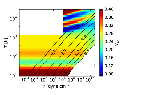
Figure 11.— Contour plot of the hydrogen adiabatic gradient $\nabla_{\rm ad}$ as a function of gas temperature and pressure. The upper right rectangle encloses the region described by the original Saumon et al. (1995) EOS tables, while the rest of the plot is our extension to lower temperatures and pressures for an equilibrium mixture of ortho- and parahydrogen. The black curves represent constant entropy adiabats with labels $\log_{10}(S)$, where $S$ [erg K^-1 g^-1] is the absolute entropy per unit mass. At high temperatures, hydrogen dissociates and ionizes, while at low temperatures the rotational states of the hydrogen molecule are only partially excited and it no longer behaves like an ideal diatomic gas. Regions in which the EOS is invalid or has not been computed are masked in white (see text).

A.2. Helium

We extend the helium EOS tables based on a similar procedure. Since helium is primarily neutral and atomic at low temperatures and pressures, we treat it as an ideal monoatomic gas and only take into account the translational component of the partition function (A4). Figure 12 shows $\nabla_{\rm ad}$ as a function of temperature and pressure for the extended EOS table.

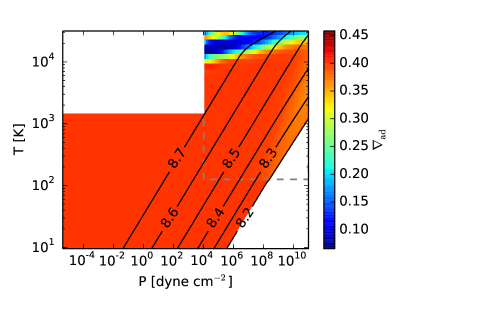
Figure 12.— Same as Figure 11 but for pure helium. Helium ionizes at $T\gtrsim 10,000$ K, but behaves as an ideal monatomic gas otherwise. We choose $T=7,000$ K as a conservative temperature cutoff above which our extension is no longer valid (masked in white). The EOS has not been computed in the lower-right region of the plot (see text).

Lastly, we combine Figures 11 and 12 to obtain EOS tables for a hydrogen-helium mixture using the procedure described in Saumon et al. (1995). Figure 1 displays results for helium mass fraction $Y=0.3$.

Appendix B Adiabatic Gradient Variations

B.1. Adiabatic Gradient during Partial Dissociation

The total internal energy of a partially dissociated gas includes contributions from the individual internal energies of the molecules and atoms, as well as from the dissociation energy. The dissociation energy depends on the dissociation fraction $x$ (i.e., the fraction of molecules that have dissociated), which can be found from the Saha equation (see e.g., Kippenhahn & Weigert 1990, Chapter 14) as a function of temperature and density,

$$\frac{x^{2}}{1-x}\propto\frac{T^{3/2}}{\rho}e^{-\chi/k_{B}T},$$ (B1)

where $\chi$=4.48 eV is the dissociation energy for molecular hydrogen (Blanksby & Ellison, 2003).

The above also holds true for ionization, with the dissociation energy replaced by ionization energy $\chi=13.6$ eV for atomic hydrogen (Mandl, 1989). From the Saha equation one can find an expression for $\rho$ as a function of $T$ and $x$, then derive the adiabatic gradient directly from its definition (Equation 4), taking into account the fact that the mean molecular weight in the ideal gas law varies with $x$, hence the pressure will not only be a function of $T$ and $\rho$ but also of $x$ (see Kippenhahn & Weigert 1990, Chapter 14.3 for a detailed derivation). The final expression for the adiabatic gradient during ionization is

$$\nabla_{\rm ad}=\frac{2+x(1-x)\Phi_{H}}{5+x(1-x)\Phi_{H}^{2}},$$ (B2)

with $\Phi_{H}\equiv\frac{5}{2}+\frac{\chi}{k_{B}T}$. The derivation of $\nabla_{\rm ad}$ during dissociation is more involved mathematically (see, e.g., Vardya 1960) and leads to a slightly more complicated final expression,

$$\nabla_{\rm ad}=\frac{1+x+\frac{x(1-x^{2})}{2}\frac{\chi}{k_{B}T}}{5x+\frac{7(1-x)}{2}+\frac{x(1-x^{2})}{2}\Big{(}\frac{\chi}{k_{B}T}\Big{)}^{2}}\,.$$ (B3)

Using Equation (B3), we recover $\nabla_{\rm ad}=2/7$ for $x=0$ (no ongoing dissociation hence hydrogen is purely molecular and diatomic) and $\nabla_{\rm ad}=2/5$ for $x=1$ (hydrogen is fully dissociated into atoms and hence monatomic). Figure 13 shows the dependence of $\nabla_{\rm ad}$ on the dissociation fraction, for $T=3000$ K, the temperature at which dissociation typically occurs (Langmuir, 1912). The adiabatic gradient drops substantially during partial dissociation, since part of the internal energy is used in dissociation rather than in increasing the temperature of the system.

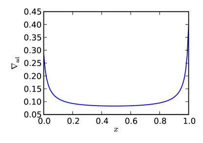
Figure 13.— Adiabatic gradient as a function of the hydrogen dissociation fraction $x$. The adiabatic gradient is $\nabla_{\rm ad}=2/7$ for pure molecular hydrogen ($x=0$) and $\nabla_{\rm ad}=2/5$ for fully atomic hydrogen ($x=1$), and drops to low values during partial dissociation.

B.2. Adiabatic Gradient during Conversion of Spin Isomers

The adiabatic gradient scales as $\nabla_{\rm ad}\sim 1/c_{\rm V}$. The translational component of the heat capacity, $c_{\rm V,t}=3\mathcal{R}/2$, is independent of temperature. As $c_{\rm V,r}$ increases, $\nabla_{\rm ad}$ declines. We can therefore understand how conversion between spin isomers affects $\nabla_{\rm ad}$ by studying the dependence on temperature of $c_{\rm V,r}$ of the ortho-para mixture.

The internal energy per unit mass and specific heat capacity associated with rotation for the individual isomers, for the equilibrium mixture, and for a fixed ortho-para ratio of 3:1 can be derived from their partition functions (see Appendix A for details), and are plotted in Figure 14 (after Farkas 1935, Figure 1). At low temperatures, parahydrogen is in the $j=0$ state and has no rotational energy, while orthohydrogen is in the $j=1$ state and has the energy of its first rotational level. Both para- and orthohydrogen, as well as their equilibrium mixture, behave like monatomic gases at low temperatures and thus have zero rotational heat capacity. This is consistent with $\nabla_{\rm ad}=2/5$ at low temperatures as seen in Figure 1. As the temperature increases, the energetically higher-lying rotational states of para- and orthohydrogen are populated and the heat capacity of both spin isomers increases as a result. We note that the heat capacity of the equilibrium mixture is not a weighted average of the heat capacities of the individual components because it takes into account both the rotational energy uptake of para- and orthohydrogen, and also the shift in their equilibrium concentrations with temperature. This results in a peak in the heat capacity of the mixture around $\sim$$50$ K, as seen in the bottom plot of Figure 14. It follows that the adiabatic gradient has to reduce, reach a minimum, then increase as the temperature rises, as shown in Figure 1. In contrast, the heat capacity for the 3:1 ortho-para ratio mixture will be a weighted average between the individual ortho- and para- components, and will hence have intermediate values between the two, as displayed in Figure 14.

Figure 15, bottom panel, shows that the atmospheric growth time may increase by a factor of $\sim$$3$ if a fixed 3:1 ortho-para ratio is assumed instead of thermal equilibrium between the hydrogen spin isomers. This enhanced growth time increases $M_{\rm crit}$.

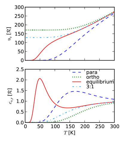
Figure 14.— Internal energy per unit mass and specific heat capacity associated with rotation for parahydrogen (dashed blue), orthohydrogen (dotted green), the equilibrium mixture (solid red) and a fixed 3:1 ortho-to-para ratio (dash-dotted light blue) as a function of temperature. After Farkas (1935), Figure 1.

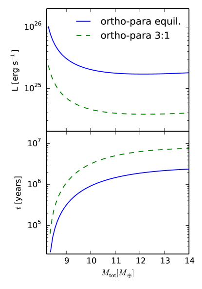
Figure 15.— Evolution of the luminosity and elapsed time during atmospheric growth around a $8M_{\oplus}$ core at 100 AU, for a realistic EOS with hydrogen spin isomers in thermal equilibrium (solid line), and with a fixed ortho-to-para ratio 3:1 (dashed line). The assumption of a fixed ortho-to-para ratio increases the runaway accretion time $t_{\rm run}$ by a factor of $\sim$$3$ compared to the equilibrium mixture.

o

Appendix C Grain growth opacity and radiative windows

The opacity of the interstellar medium is reasonably well constrained and approximate analytic expressions for the Rosseland mean opacity as a function of temperature and density are derived in Bell & Lin (1994). For low temperatures ($T\lesssim 100$ K) at which ice grains are present, opacity scales with temperature as $\kappa\sim T^{2}$. Sublimation of ice grains at $\sim$$150$ K and of metal grains at $\sim$$1000$ K results in sharp opacity drops. This is shown in Figure 16 for a gas density $\rho=10^{-8}$ g cm^-3, which is typical for the outer regions of protoplanetary disks. Semenov et al. (2003) calculate Rosseland mean opacities in protoplanetary disks for grains of different sizes and structure. As shown in Figure 16, their results are in good agreement with Bell & Lin (1994). However, Semenov et al. (2003) do not take grain growth into account, which is likely to occur in protoplanetary disks, particularly at the late times when cores form. D’Alessio et al. (2001) compute wavelength dependent opacities for a range of maximum particle sizes and different size distributions. Figure 16 shows the integrated Rosseland mean opacity for a maximum particle size of 1 cm and a power law differential size distribution $dN/ds\propto s^{-p}$, with $s$ the grain size and $p=3.5$ for a standard collisional cascade and $p=2.5$ when coagulation is taken into account. We see in Figure 16 that this yields a mean opacity that is both lower and less sensitive to temperature, when compared to Bell & Lin (1994) or Semenov et al. (2003). However, D’Alessio et al. (2001) only computes opacities for temperatures less than the dust sublimation temperature, appropriate for current observations of dust in protoplanetary disks. As we see in Figure 16, the opacity dramatically decreases during dust sublimation. We thus use the Bell & Lin (1994) opacities for $T\gtrsim 1000$ K, ensuring that they smoothly match the D’Alessio et al. (2001) opacities for lower temperatures.

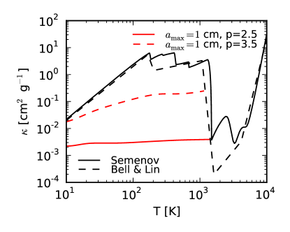
Figure 16.— Rosseland mean opacity of dust grains as a function of temperature for different opacity assumptions. The dashed black curve shows the Bell & Lin (1994) analytic ISM opacity for $\rho=10^{-8}$ g cm^-3. The solid black curve shows the tabulated opacity of Semenov et al. (2003) for a dust composition of ’normal’ silicates. The dashed red curve shows the D’Alessio et al. (2001) opacity, which takes grain growth into account, for a maximum particle size of 1 cm and a standard collisional cascade grain size distribution ($p=3.5$). The solid red curve is the same as the dashed red curve, but it accounts for coagulation ($p=2.5$).

The significant opacity drop due to the sublimation of ice and metal grains lowers the radiative temperature gradient $\nabla_{\rm rad}$, which may result in one or more inner radiative layers inside the atmosphere of a protoplanet. This is displayed in Figure 17: depending on the semimajor axis and core mass, the opacity drop will generate no radiative window (top panel), one radiative window (middle panel), or two radiative windows (bottom panel).

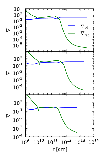
Figure 17.— Snapshots of the radiative and adiabatic gradient as a function of the radial coordinate, for planets with different core masses forming at various locations in the disk. The nebular gas is described by a realistic EOS, with a standard collisional cascade size distribution ($p=3.5$). The sharp drop in opacity due to dust sublimation may generate one or more radiative windows. Top panel: no radiative window for $a=100$ AU and $M_{\rm c}=3M_{\oplus}$. Middle panel: the sharp opacity decrease produces one radiative window for $a=50$ AU and $M_{\rm c}=5M_{\oplus}$. Bottom panel: the decrease in opacity results in two radiative windows for $a=20$ AU and $M_{\rm c}=3M_{\oplus}$.

Our idealization of a constant $L$ with radius may be challenged by the presence of radiative windows. While the structure of convective regions is unaffected by $L$, the structure of radiative windows depends on $L$. Fortunately, the assumption of constant luminosity remains reasonable if most of the luminosity is generated in the innermost convective region of the envelope. We can check whether this is true a posteriori by using the local energy equation,

$$\frac{\partial L}{\partial m}=-T\frac{\partial S}{\partial t},$$ (C1)

and integrating it between $M_{\rm c}$ and $M_{\rm{RCB_{1}}}$, where $\rm{RCB_{1}}$ is the innermost RCB. This luminosity can be as little as half of the assumed fixed atmospheric luminosity $L$.

Self-consistently calculating $L(r)$ is not feasible for our code. Instead, we note that since $\partial S/\partial t$ is fixed in convective regions (Arras & Bildsten, 2006), the luminosity profile is more centrally concentrated than $L\propto m$, which can be implemented simply. We calculated example profiles using $L\propto m$ and found that though this luminosity scaling may move the location of the outermost RCB, it does not substantially change the luminosity emerging at the top of the atmosphere or the time evolution.

References

- Alibert et al. (2005) Alibert, Y., Mordasini, C., Benz, W., & Winisdoerffer, C. 2005, A&A, 434, 343
- Arras & Bildsten (2006) Arras, P. & Bildsten, L. 2006, ApJ, 650, 394
- Bai & Goodman (2009) Bai, X.-N. & Goodman, J. 2009, ApJ, 701, 737
- Beckwith & Sargent (1991) Beckwith, S. V. W. & Sargent, A. I. 1991, ApJ, 381, 250
- Beckwith et al. (1990) Beckwith, S. V. W., Sargent, A. I., Chini, R. S., & Guesten, R. 1990, AJ, 99, 924
- Bell & Lin (1994) Bell, K. R. & Lin, D. N. C. 1994, ApJ, 427, 987
- Blanksby & Ellison (2003) Blanksby, S. J. & Ellison, G. B. 2003, Acc. Chem. Res., 36, 255
- Bodenheimer et al. (1980) Bodenheimer, P., Grossman, A. S., Decampli, W. M., Marcy, G., & Pollack, J. B. 1980, Icarus, 41, 293
- Bodenheimer & Pollack (1986) Bodenheimer, P. & Pollack, J. B. 1986, Icarus, 67, 391
- Boley et al. (2007) Boley, A. C., Hartquist, T. W., Durisen, R. H., & Michael, S. 2007, ApJ, 656, L89
- Chiang & Youdin (2010) Chiang, E. & Youdin, A. N. 2010, Annual Review of Earth and Planetary Sciences, 38, 493
- Conrath & Gierasch (1984) Conrath, B. J. & Gierasch, P. J. 1984, Icarus, 57, 184
- D’Alessio et al. (2001) D’Alessio, P., Calvet, N., & Hartmann, L. 2001, ApJ, 553, 321
- D’Angelo & Bodenheimer (2013) D’Angelo, G. & Bodenheimer, P. 2013, ApJ, 778, 77
- D’Angelo et al. (2011) D’Angelo, G., Durisen, R. H., & Lissauer, J. J. Giant Planet Formation, ed. S. Piper, 319–346
- Dohnanyi (1969) Dohnanyi, J. S. 1969, J. Geophys. Res., 74, 2531
- Farkas (1935) Farkas, A. 1935, Orthohydrogen, Parahydrogen and Heavy Hydrogen
- Fouchet et al. (2003) Fouchet, T., Lellouch, E., & Feuchtgruber, H. 2003, Icarus, 161, 127
- Fukutani & Sugimoto (2013) Fukutani, K. & Sugimoto, T. 2013, Progress In Surface Science, 88, 279
- Glassgold et al. (1997) Glassgold, A. E., Najita, J., & Igea, J. 1997, ApJ, 480, 344
- Goldreich et al. (2004) Goldreich, P., Lithwick, Y., & Sari, R. 2004, ARA&A, 42, 549
- Graboske et al. (1969) Graboske, H. C., Harwood, D. J., & Rogers, F. J. 1969, Physical Review, 186, 210
- Hori & Ikoma (2010) Hori, Y. & Ikoma, M. 2010, ApJ, 714, 1343
- Hubickyj et al. (2005) Hubickyj, O., Bodenheimer, P., & Lissauer, J. J. 2005, Icarus, 179, 415
- Huestis (2008) Huestis, D. L. 2008, Planet. Space Sci., 56, 1733
- Ida et al. (2013) Ida, S., Lin, D. N. C., & Nagasawa, M. 2013, ApJ, 775, 42
- Ikoma et al. (2000) Ikoma, M., Nakazawa, K., & Emori, H. 2000, ApJ, 537, 1013
- Inutsuka (2012) Inutsuka, S.-i. 2012, Progress of Theoretical and Experimental Physics, 2012, 010000
- Jayawardhana et al. (1999) Jayawardhana, R., Hartmann, L., Fazio, G., Fisher, R. S., Telesco, C. M., & Piña, R. K. 1999, ApJ, 521, L129
- Kippenhahn & Weigert (1990) Kippenhahn, R. & Weigert, A. 1990, Stellar Structure and Evolution
- Kittel et al. (1981) Kittel, C., Kroemer, H., & Landsberg, P. T. 1981, Nature, 289, 729
- Langmuir (1912) Langmuir, I. 1912, J. Am. Chem. Soc., 34, 860
- Larson (1969) Larson, R. B. 1969, MNRAS, 145, 271
- Lique et al. (2012) Lique, F., Honvault, P., & Faure, A. 2012, J. Chem. Phys., 137, 154303
- Lique et al. (2014) —. 2014, ArXiv e-prints, arXiv:1402.5292
- Mandl (1989) Mandl, F. 1989, Statistical Physics, 2nd Edition
- Marois et al. (2008) Marois, C., Macintosh, B., Barman, T., Zuckerman, B., Song, I., Patience, J., Lafrenière, D., & Doyon, R. 2008, Science, 322, 1348
- Milenko et al. (1997) Milenko, Y. Y., Sibileva, R. M., & Strzhemechny, M. A. 1997, Journal of Low Temperature Physics, 107, 77
- Militzer & Hubbard (2013) Militzer, B. & Hubbard, W. B. 2013, ApJ, 774, 148
- Mizuno et al. (1978) Mizuno, H., Nakazawa, K., & Hayashi, C. 1978, Progress of Theoretical Physics, 60, 699
- Mordasini (2014) Mordasini, C. 2014, A&A, 572, A118
- Mordasini et al. (2012) Mordasini, C., Alibert, Y., Klahr, H., & Henning, T. 2012, A&A, 547, A111
- Mordasini et al. (2014) Mordasini, C., Klahr, H., Alibert, Y., Miller, N., & Henning, T. 2014, ArXiv e-prints
- Movshovitz et al. (2010) Movshovitz, N., Bodenheimer, P., Podolak, M., & Lissauer, J. J. 2010, Icarus, 209, 616
- Nettelmann et al. (2012) Nettelmann, N., Becker, A., Holst, B., & Redmer, R. 2012, ApJ, 750, 52
- Nettelmann et al. (2008) Nettelmann, N., Holst, B., Kietzmann, A., French, M., Redmer, R., & Blaschke, D. 2008, ApJ, 683, 1217
- Ormel (2013) Ormel, C. W. 2013, MNRAS, 428, 3526
- Ormel (2014) —. 2014, ApJ, 789, L18
- Pachucki & Komasa (2008) Pachucki, K. & Komasa, J. 2008, Phys. Rev. A, 77, 030501
- Papaloizou & Nelson (2005) Papaloizou, J. C. B. & Nelson, R. P. 2005, A&A, 433, 247
- Papaloizou & Terquem (1999) Papaloizou, J. C. B. & Terquem, C. 1999, ApJ, 521, 823
- Paxton et al. (2011) Paxton, B., Bildsten, L., Dotter, A., Herwig, F., Lesaffre, P., & Timmes, F. 2011, ApJS, 192, 3
- Paxton et al. (2013) Paxton, B., Cantiello, M., Arras, P., Bildsten, L., Brown, E. F., Dotter, A., Mankovich, C., Montgomery, M. H., Stello, D., Timmes, F. X., & Townsend, R. 2013, ApJS, 208, 4
- Pérez et al. (2012) Pérez, L. M., Carpenter, J. M., Chandler, C. J., Isella, A., Andrews, S. M., Ricci, L., Calvet, N., Corder, S. A., Deller, A. T., Dullemond, C. P., Greaves, J. S., Harris, R. J., Henning, T., Kwon, W., Lazio, J., Linz, H., Mundy, L. G., Sargent, A. I., Storm, S., Testi, L., & Wilner, D. J. 2012, ApJ, 760, L17
- Perez-Becker & Chiang (2011) Perez-Becker, D. & Chiang, E. 2011, ApJ, 727, 2
- Piso & Youdin (2014) Piso, A.-M. A. & Youdin, A. N. 2014, ApJ, 786, 21
- Pollack et al. (1996) Pollack, J. B., Hubickyj, O., Bodenheimer, P., Lissauer, J. J., Podolak, M., & Greenzweig, Y. 1996, Icarus, 124, 62
- Pollack et al. (1985) Pollack, J. B., McKay, C. P., & Christofferson, B. M. 1985, Icarus, 64, 471
- Rafikov (2006) Rafikov, R. R. 2006, ApJ, 648, 666
- Rafikov (2011) —. 2011, ApJ, 727, 86
- Saumon et al. (1995) Saumon, D., Chabrier, G., & van Horn, H. M. 1995, ApJS, 99, 713
- Semenov et al. (2003) Semenov, D., Henning, T., Helling, C., Ilgner, M., & Sedlmayr, E. 2003, A&A, 410, 611
- Stevenson (1982) Stevenson, D. J. 1982, Planet. Space Sci., 30, 755
- Takahashi (2001) Takahashi, J. 2001, ApJ, 561, 254
- Thompson (2006) Thompson, M. J. 2006, An introduction to astrophysical fluid dynamics
- Turner et al. (2010) Turner, N. J., Carballido, A., & Sano, T. 2010, ApJ, 708, 188
- Vardya (1960) Vardya, M. S. 1960, ApJS, 4, 281
- Walmsley et al. (2004) Walmsley, C. M., Flower, D. R., & Pineau des Forêts, G. 2004, A&A, 418, 1035
- Wuchterl (1993) Wuchterl, G. 1993, Icarus, 106, 323