Stellar masses from the CANDELS survey: the GOODS-South and UDS fields

Abstract

We present the public release of the stellar mass catalogs for the GOODS-S and UDS fields obtained using some of the deepest near-IR images available, achieved as part of the Cosmic Assembly Near-infrared Deep Extragalactic Legacy Survey (CANDELS) project. We combine the effort from ten different teams, who computed the stellar masses using the same photometry and the same redshifts. Each team adopted their preferred fitting code, assumptions, priors, and parameter grid. The combination of results using the same underlying stellar isochrones reduces the systematics associated with the fitting code and other choices. Thanks to the availability of different estimates, we can test the effect of some specific parameters and assumptions on the stellar mass estimate. The choice of the stellar isochrone library turns out to have the largest effect on the galaxy stellar mass estimates, resulting in the largest distributions around the median value (with a semi interquartile range larger than 0.1 dex). On the other hand, for most galaxies, the stellar mass estimates are relatively insensitive to the different parameterizations of the star formation history. The inclusion of nebular emission in the model spectra does not have a significant impact for the majority of galaxies (less than a factor of 2 for $\sim$80% of the sample). Nevertheless, the stellar mass for the subsample of young galaxies (age $<100$ Myr), especially in particular redshift ranges (e.g., $2.2<z<2.4$, $3.2<z<3.6$, and $5.5<z<6.5$), can be seriously overestimated (by up to a factor of 10 for $<20$ Myr sources) if nebular contribution is ignored.

I. Introduction

Reliable stellar mass estimates are of crucial importance to achieve a better understanding of galaxy evolution. Stellar mass estimates are complementary to other measures of galaxy stellar populations, such as star formation rates (SFRs) and age. They tend to be more accurate than estimates of SFR, which suffer from larger uncertainties due to degeneracies between dust, age, and metallicity.

Nevertheless, stellar mass estimates are also potentially affected by systematic uncertainties. The latter primarily originate from our limited knowledge of several properties of the stellar populations, such as their metallicity, which is not well constrained by a fit to broad-band photometry (e.g., Castellano et al., 2014), the extinction curve, or some phases of stellar evolution. The most striking example is the thermally pulsating asymptotic giant branch (TP-AGB) phase (Maraston, 2005; Marigo et al., 2008) – the modeling of which is still debated (Zibetti et al., 2013) – which has a relevant contribution to the near-IR emission of galaxies dominated by intermediate-age stellar populations ($\sim$1 Gyr). Another difficulty when estimating galaxy stellar masses is properly reconstructing their star formation histories (SFHs), which are usually approximated by simple (but not necessarily appropriate) parametric functions.

Despite the systematics discussed above, high quality photometry and accurate redshifts may significantly improve the reliability of the measured stellar masses. The Cosmic Assembly Near-infrared Deep Extragalactic Legacy Survey (CANDELS, Koekemoer et al. 2011; Grogin et al. 2011, PIs: S. Faber, H. Ferguson) is of great help in this regard, thanks to its exquisite quality near-IR photometry taken with the WFC3 camera on board the Hubble Space Telescope (HST). CANDELS observations include some of the deepest images in the visible and near-IR ever achieved over a wide area, and have been complemented with the best auxiliary photometry available in the mid-IR with Spitzer Space Telescope and in the ultraviolet with ground-based observations. Thanks to the combination of depth and area covered, stellar masses from the CANDELS project can greatly improve our knowledge of the galaxy stellar mass assembly process, both in a statistical sense (e.g., they allow a robust measure of the galaxy stellar mass functions; Grazian et al. 2015, G15 hereafter, Duncan et al. 2014) and for dedicated analyses of interesting, faint and distant sources.

The aim of this paper is to present and accompany the release of CANDELS stellar mass catalogs for the Great Observatories Origins Deep Survey-South (GOODS-S, Giavalisco et al. 2004) and UKIRT Infrared Deep Sky Survey (UKIDSS) Ultra-Deep Survey (UDS, Lawrence et al. 2007) fields. This is the third of a series of papers that combine the effort of several teams within the CANDELS collaboration to achieve an improved result. In the first paper, Dahlen et al. (2013) (D13 hereafter) presented and compared photometric redshifts computed by eleven teams and demonstrated that the combination of multiple results is able to reduce the scatter and outlier fraction in the photometric redshifts. In the second work in the series (Mobasher et al., 2015, M15 hereafter), we performed a comprehensive study of stellar mass measurements and analyzed the main sources of uncertainties and the associated error budget by using mock galaxy catalogs based on semi-analytical models as well as observed catalogs. Biases of the ten different fitting techniques turned out to be relatively small, and tended to be confined to galaxies younger than $\sim$100 Myr, where models with a fine spacing of the model grid in age and extinction appeared to perform best. The faintest and lowest signal-to-noise ratio (S/N) galaxies were found to be affected by the largest scatter. Degeneracies between stellar mass, age, and extinction were disentangled.

In this work we present and publicly release stellar masses computed from the official CANDELS photometric and redshift catalogs by ten teams, each adopting their preferred assumptions in terms of SFH, stellar modeling and stellar parameters. We then combine these estimates to suppress the effect of systematics deriving from the choice of specific assumptions and priors in each of the methods.

The paper is organized as follows: Section II presents CANDELS photometric and redshift catalogs; Section III describes how stellar masses were estimated by the different teams, whose results are compared in Section IV; the official CANDELS stellar masses are presented in Section V; finally, we summarize the main results in Section VI. All magnitudes are in the AB system, and the following cosmology has been adopted: H₀ = 70 km/s/Mpc, $\Omega_{\small M}$ $=$ 0.3, and $\Omega_{\Lambda}$ = 0.7.

II. Data set

II.1. GOODS-S and UDS multiwavelength catalogs

The CANDELS multiwavelength group has adopted a standardized method to build catalogs in the CANDELS fields. Sources are extracted from the CANDELS F160W mosaic using SExtractor. Total fluxes of the sources in the high-resolution HST bands (WFC3 and ACS) are derived from the aperture-corrected isophotal colors from SExtractor, run in dual mode on PSF-matched images (where the PSF is the Point Spread Function). The photometry of the lower-resolution dataset (e.g., ground-based and Spitzer) is derived using the template-fitting software TFIT (Laidler et al., 2007; Papovich et al., 2001). In brief, TFIT uses the a-priori information on the source location and surface brightness profile on the F160W image to measure its photometry on the low-resolution image. We refer the reader to Galametz et al. (2013) for details on the adopted catalog building procedure.

The dataset available for each CANDELS field is rich but significantly varies from field-to-field. As such, the multiwavelength catalogs of GOODS-S and UDS contain different bands and data depths:

CANDELS-GOODS-S

The GOODS-S catalog contains 34930 sources. The total area of $\sim 170$ square arcmin was observed by WFC3 with a mixed strategy, combining CANDELS data in a deep (central one-third of the field) and a wide (southern one-third) region with ERS (Windhorst et al., 2011) (northern one-third) and HUDF09 (Bouwens et al., 2010) observations. The F160W mosaic reaches a 5$\sigma$ limiting magnitude (within an aperture of radius 0.17 arcsec) of 27.4, 28.2, and 29.7 in the CANDELS wide, deep, and HUDF regions, respectively. The multiwavelength catalog includes 18 bands: in addition to the ERS/WFC3 and CANDELS/WFC3 data in the $F105W$/$F125W$/$F140W$/$F160W$ filters, it also includes data from UV ($U$ band from both CTIO/MOSAIC and VLT/VIMOS), optical (HST/ACS F435W, F606W, F775W, F814W, and F850LP), and infrared (HST/WFC3 F098M, VLT/ISAAC $K_{s}$, VLT/HAWK-I $K_{s}$, and Spitzer/IRAC 3.6, 4.5, 5.8, 8.0$\mu$m) observations. See Guo et al. (2013) for a summary of the GOODS-S UV-to-mid-IR dataset and corresponding survey references.

CANDELS-UDS

The UDS catalog contains $35932$ sources distributed over an area of $\sim 201.7$ square arcmin (roughly a rectangular field of view of $22.3^{\prime}\times 9^{\prime}$). The F160W CANDELS image reaches a 5$\sigma$ limiting depth of 27.45 within an aperture of radius 0.20 arcsec. The multiwavelength catalog includes 19 bands: the CANDELS data (WFC3 $F125W$/$F160W$ and ACS $F606W$/$F814W$ data), $U$ band data from CFHT/Megacam, $B$, $V$, $R_{c}$, $i^{\prime}$ and $z^{\prime}$ band data from Subaru/Suprime-Cam, $Y$ and $K_{s}$ band data from VLT/HAWK-I, $J$, $H$ and $K$ bands data from UKIDSS (Data Release 8), and Spitzer/IRAC data ($3.6$, $4.5$ from SEDS, Ashby et al. 2013, $5.8$ and $8.0\mu$m from SpUDS). The first released version of the catalog contains a list of about $210$ sources with reliable spectroscopic redshifts that we have extended in the present analysis with new redshifts derived from the VLT VIMOS/FORS2 spectroscopic campaigns (Bradshaw et al. 2013, McLure et al. 2013 and Almaini et al. in prep.) and the MAGELLAN/IMACS spectroscopy presented in Appendix A. See Galametz et al. (2013) for a summary of the UDS UV-to-mid-IR dataset and corresponding survey references.

II.2. Redshifts

CANDELS multiwavelength catalogs were cross-matched with a collection of publicly available spectroscopic sources in both fields and with the Magellan spectroscopy in UDS that is presented here for the first time (see Appendix A). $\sim 10\%$ and $\sim 2\%$ of sources have a spectroscopic counterpart in GOODS-S and UDS, respectively. In addition to the redshift value, the released catalogs report the spectral quality and the original parent spectroscopic survey. Once spectroscopic stars and poor quality spectra have been removed, the fraction of galaxies with reliable spectroscopic redshifts are $\sim 6\%$ and $\sim 1\%$ in the two fields, respectively. If only H${}_{160}<24$ sources are considered, the spectroscopic fraction is $\sim 29\%$ and $\sim 8\%$, respectively.

Photometric redshifts have been computed for all CANDELS sources using the official multiwavelength photometry catalogs described above. Briefly, photometric redshifts are based on a hierarchical Bayesian approach that combines the full PDF(z) distributions derived by six CANDELS photo-$z$ investigators. The 68% and 95% confidence intervals, also included in the stellar mass catalogs, are calculated from the final redshift probability distribution. The techniques adopted to derive the official CANDELS photometric redshifts, as well as the individual values from the various participants, are described in details by D13, and the photometric redshift catalogs of both fields will be made available in a forthcoming paper (Dahlen et al. in prep.).

II.3. Data selection

We removed from the present analysis all objects flagged for having bad photometry (see Guo et al. 2013 and Galametz et al. 2013). This information is available in the photometric catalogs as well in the catalogs we release with the present work.

Stars have been classified either spectroscopically or photometrically, and have been removed from the sample. 151 and 47 sources were identified as spectroscopic stars in GOODS-S and UDS, respectively. No stellar mass nor any other parameter is provided in the catalogs for these sources. Photometric stellar candidates have been selected through the morphological information provided by SExtractor on the F160W band (CLASS_STAR$>$0.95) combined with the requirement that S/N is larger than 20, which ensures reliability of the CLASS_STAR parameter. The total number of high S/N point-like candidates is 174 in GOODS-S and 224 in UDS. Fainter point-like sources are not flagged as stars due to unreliability of the morphological criterion for low S/N sources, and conservatively included in this analysis.

Finally, CANDELS catalogs have been cross-matched with X-ray sources from the Chandra 4Ms catalogs of Xue et al. (2011) and Rangel et al. (2013) (see Hsu et al., 2014) in the GOODS-S field and with the XMM-Newton sample of Ueda et al. (2008) in the UDS field. We flag X-ray selected AGN candidates and do not use them in the comparisons shown in this paper. We remind the reader that a non detection in X-ray does not prove that the source does not host an AGN, because AGN detection depends on the depth of the X-ray survey and on the level of obscuration. Dedicated works on IR AGN in all the CANDELS fields are in preparation within the CANDELS collaboration.

Although we exclude AGNs from the present comparison, masses for AGN candidates have been computed using the same technique as for non active galaxies and are released in the catalogs. In GOODS-S they were computed by fixing the redshift to the photometric value obtained by fitting the photometry with hybrid templates, as described by Hsu et al. (2014). This approach provides reliable mass estimates for the large majority of obscured AGNs, whose SED is dominated by the stellar component (Santini et al., 2012a). We caution that the stellar mass estimate may not recover the true value for bright unobscured AGNs, where ad-hoc techniques should be adopted (Merloni et al., 2010; Santini et al., 2012a; Bongiorno et al., 2012). However, these sources make up only 8% of the AGN sample in GOODS-S (Hsu et al., 2014), which, due to the small area, only rarely includes very bright AGNs. No dedicated photometric redshifts for AGNs were computed in UDS. These are going to be presented in a more complete future work on AGNs in all CANDELS fields.

III. Stellar mass estimates

III.1. The estimate of the stellar mass

Stellar masses are commonly estimated by fitting the observed multiwavelength photometry with stellar population synthesis templates (e.g., Fioc & Rocca-Volmerange 1997, Bruzual & Charlot 2003, BC03 hereafter, Maraston 2005, Bruzual 2007, CB07 hereafter, Conroy & Gunn 2010, see Conroy 2013 for a review).

The most widely used metric for goodness of fit is $\chi^{2}$. A grid for the free parameters must be set, and model spectra, computed by fixing these parameters to the values in each step of the grid, are compared with observed fluxes. The best-fit parameters are either provided by the template minimizing $\chi^{2}$ or computed as the median of the Probability Distribution Function (PDF). For some codes, the PDF of stellar mass is computed from the $\chi^{2}$ contingency tables; for others, the likelihood contours are determined in all the fitting parameters using Markov Chain Monte Carlo (MCMC) sampling, and the stellar mass PDF is determined by marginalizing over the other parameters. In this case, parameters are allowed to vary on a continuous space, which is explored by means of a random walk. In the case of the SpeedyMC code (Acquaviva et al., 2012), used by one of the participating teams, multi-linear interpolation between the pre-computed spectra is used to compute the model SEDs. The final best-fit parameters are the average of the posterior PDF, which is proportional to the frequency of visited locations.

Free parameters in the models include stellar metallicity, age (defined as time since the onset of star formation), dust reddening, and the parameters describing the SFH of the galaxy. Moreover, several assumptions have to be made, such as the choice of the initial stellar mass function (IMF) and the extinction law.

One of the most important assumptions for shaping the final templates is the parameterization of the SFH. The star formation process in galaxies can be very complicated and may have a stochastic nature. In the attempt of reproducing the real SFH, several simple analytic functions are usually adopted. The most popular functions are:

• exponentially declining laws, the so-called $\tau$ models (or direct-$\tau$ models): $\psi(t)\propto exp(-t/\tau)$;

• exponentially increasing laws, also called inverted-$\tau$ models: $\psi(t)\propto exp(t/\tau)$;

• constant SFH: $\psi(t)=const$;

• instantaneous bursts: $\psi(t)\propto\delta(t_{0})$.

Some more complicated shapes include:

• the so-called delayed-$\tau$ models, i.e., rising-declining laws: e.g., $\psi(t)\propto t/\tau^{2}\cdot exp(-t/\tau)$ or $\psi(t)\propto t^{2}/\tau\cdot exp(-t/\tau)$;

• truncated SFH: $\psi(t)=const$ if $t<t_{0}$, $\psi(t)=0$ otherwise;

and even more complex functional forms that have been proposed by previous works (e.g., Behroozi et al., 2013; Simha et al., 2014).

III.2. Stellar mass estimates within CANDELS

In order to investigate possible systematics due to different assumptions, ten teams within the CANDELS collaboration computed the stellar masses on the same released catalogs and on the same redshifts. Good quality spectroscopic redshifts were used when available, and the official CANDELS Bayesian photometric redshifts (Dahlen et al. in prep.) were adopted for all other galaxies.

Following the same notation as D13 and M15, we designate each team with a code. Codes are composed of a number identifying the team PI, of a letter indicating the stellar templates used, and if appropriate the subscript _τ to indicate that purely exponentially decreasing $\tau$ models have been assumed to parameterize the SFH.

Each of the teams was free to choose their favorite assumptions and set their preferred parameter grid. Although most of the teams adopted BC03 stellar templates, other libraries were also used. Table 1 summarizes, for each of the participant teams, the fitting technique, the code used to fit the data, the stellar templates adopted, the main assumptions in terms of IMF, SFH, extinction law, the ranges of the parameter grid employed, and the priors applied to the template library. The grid steps differ one from the other, as indicated in Table 1, and may in some cases vary over the range covered.

Most mass estimates presented in this work adopt a Calzetti et al. (2000) attenuation curve, while one method (Method 6a_τ) treats the extinction curve as a free parameter, and allows it to vary between a Calzetti et al. (2000) and a SMC (Prevot et al., 1984) one.

Three teams also include nebular emission lines and nebular continuum in one case in addition to stellar emission in the model templates:

• Method 4b: the strength of the H$\beta$ line is computed from the number of ionizing photons for a given age and metallicity assuming Case B recombination and null escape fraction, and line ratios for 119 lines are taken from the Cloudy models of Inoue (2011) (see Salmon et al. 2015);

• Method 11a_τ: the addition of Ly$\alpha$, [OII], [OIII], H$\alpha$ and H$\beta$ is done following the recipe of Ilbert et al. (2009), who adopted the relation from Kennicutt (1998) between UV luminosity, SFR and [OII] flux, and applied line ratios to predict the flux in the other lines;

• Method 14a: the flux from the nebular continuum and line emission is included by tracking the number of Lyman-continuum photons and assuming Case B recombination and null escape fraction, and modeling the empirical line intensities relative to H$\beta$ for H, He, C, N, O, S as a function of metallicity (Anders & Fritze-v. Alvensleben, 2003; Schaerer & de Barros, 2009; Acquaviva et al., 2011).

Not all participants computed the stellar masses for both fields. In the end, we present 9 different sets of stellar masses for the GOODS-S field and 9 for the UDS field.

In addition to their preferred mass estimate, some of the teams also provided further results based on different assumptions. Although we will not use these to compute the final stellar mass values, we present them in Table 4 in Appendix B, and we will use them to test how specific parameters affect the best-fit result in the next section.

All these stellar mass estimates are included as electronic tables on the online edition of this publication.

Table 1 Summary of the assumptions adopted to compute the stellar masses in CANDELS.

	Method 2aτ	Method 2dτ	Method 4b	Method 6aτ	Method 10c
PI	G. Barro	G. Barro	S. Finkelstein	A. Fontana	J. Pforr
fitting method	min $\chi^{2}$	min $\chi^{2}$	min $\chi^{2}$	min $\chi^{2}$	min $\chi^{2}$
code	FAST v0.9b	Rainbow	own code	zphot	HyperZ
stellar templates	BC03	PEGASE v1.0	CB07	BC03e	M05
IMF	Chabrier	Salpeter	Salpeter	Chabrier	Chabrier
SFH	$\tau$	$\tau$i	$\tau$i + inv-$\tau$	$\tau$i	$\tau$i + trunc.
			+ const.		+ const.l
log ($\tau$/yr)	8.5–10.0	6.0–11.0	5.0–11.0	8.0–10.2	8.0, 8.5, 9.0
step	0.2	0.1	6 steps	9 steps
log ($\tau^{INV}$/yr)			8.5, 9.0, 10.0
log ($t_{0}$/yr)					8.0, 8.5, 9.0
metallicity [Z⊙]	1	0.005, 0.02, 0.2,	0.02, 0.2, 0.4, 1	0.02, 0.2, 1, 2.5	0.2, 0.5, 1, 2.5
		0.4, 1, 2.5, 5
log (age/yr)	7.6–10.1	6.0–10.1	6.0–10.1	7.0–10.1	8.0 – 10.3
stepm	0.1	60 steps	40 steps	110 steps	221 steps
extinction law	Calzetti	Calzetti	Calzetti	Calzetti + SMC	—
extinction E(B-V)	0.0–1.0	0.00–1.24	0.0–0.8	0.0–1.1	0.0
step	0.025	0.025	0.02	0.05
nebular emission	no	no	yes	no	no
priors		p	p	p	p
reference	1	2	3	4	5

Note. — References. (1) Barro et al. (2013) ; (2) Pérez-González et al. (2008); (3) Finkelstein et al. (2012); (4) Fontana et al. (2006); (5) Daddi et al. (2005); Maraston et al. (2006); Pforr et al. (2012, 2013).

Table 1 (continued)

	Method 11aτ	Method 12a	Method 13aτ	Method 14a	Method 15a
PI	M. Salvato	T. Wiklind	S. Wuyts	B. Lee	S.-K. Lee
fitting method	median of the	min $\chi^{2}$	min $\chi^{2}$	MCMC	min $\chi^{2}$
	mass PDF
code	Le Phare	WikZ	FASTa v0.8b	SpeedyMC	own code
stellar templates	BC03e	BC03e	BC03e	BC03e	BC03e
IMF	Chabrier	Chabrier	Chabrier	Chabrier	Chabrier
SFH	$\tau$i	del-$\tau$	$\tau$i	$\tau$i + del-$\tau$w + const.l	del-$\tau$w
				+ lin. incr.
log ($\tau$/yr)	8.0–10.5	-$\infty$ – 9.3	8.5–10.0	7.0–9.7	8.0–10.0
stepm	9 steps	9 steps	0.1	—	14 steps
metallicity [Z⊙]	0.4, 1	0.2, 0.4, 1, 2.5	1	1	0.2, 0.4, 1, 2.5
log (age/yr)	7.0–10.1	7.7–9.8	7.7–10.1	8.0–10.1	7.7–10.1
stepm	57 steps	24 steps	0.1	—	64 steps
extinction law	Calzetti	Calzetti	Calzetti	Calzetti	Calzetti
extinction E(B-V)	0.0–0.5	0.0–1.0	0.0–1.0	0.0–1.0	0.0–1.5
step	0.1	0.025	0.025	—	0.025
nebular emission	yes	no	no	yes	no
priors	p	p	p	p	p
reference	6	7	8	9	10

Note. — References. (6) Ilbert et al. (2010); (7) Wiklind et al. (2008, 2014); (8) Wuyts et al. (2011); (9) B. Lee et al., in prep.; (10) Lee et al. (2010).

IV. Comparison of different assumptions

This section discusses the overall agreement/disagreement and then the effects of the SFH and of including nebular emission. For a more detailed and systematic discussion about the uncertainties in the stellar mass estimates of different methods, we refer the reader to M15.

IV.1. Overall comparison

Because no “true” mass against which to compare all the others is available, we start by comparing each mass estimate with the median value. This median was computed for each galaxy by considering all sets of stellar masses after rescaling them to the same Chabrier IMF (as this is the IMF adopted by all but two of the teams): following Santini et al. (2012b), we subtract 0.24 dex from stellar masses computed assuming the Salpeter IMF. To deal with the low number of measurements available to compute the median, we adopt the Hodges-Lehmann estimator, defined as the median value of the means in the linear space of each pair of estimates in the sample:

$$M_{*}={\rm median}\left(\frac{x_{i}+x_{j}}{2}\right),$$ (1)

We used a bootstrap procedure (with 10 times the number of measurements iterations) to randomly choose the pairs $i$ and $j$, rather than using all possible values. This statistical estimator has the robustness of an ordinary median but smaller uncertainty. We refer to this Hodges-Lehmann mean value as $M_{*}^{\rm MEDIANall}$.

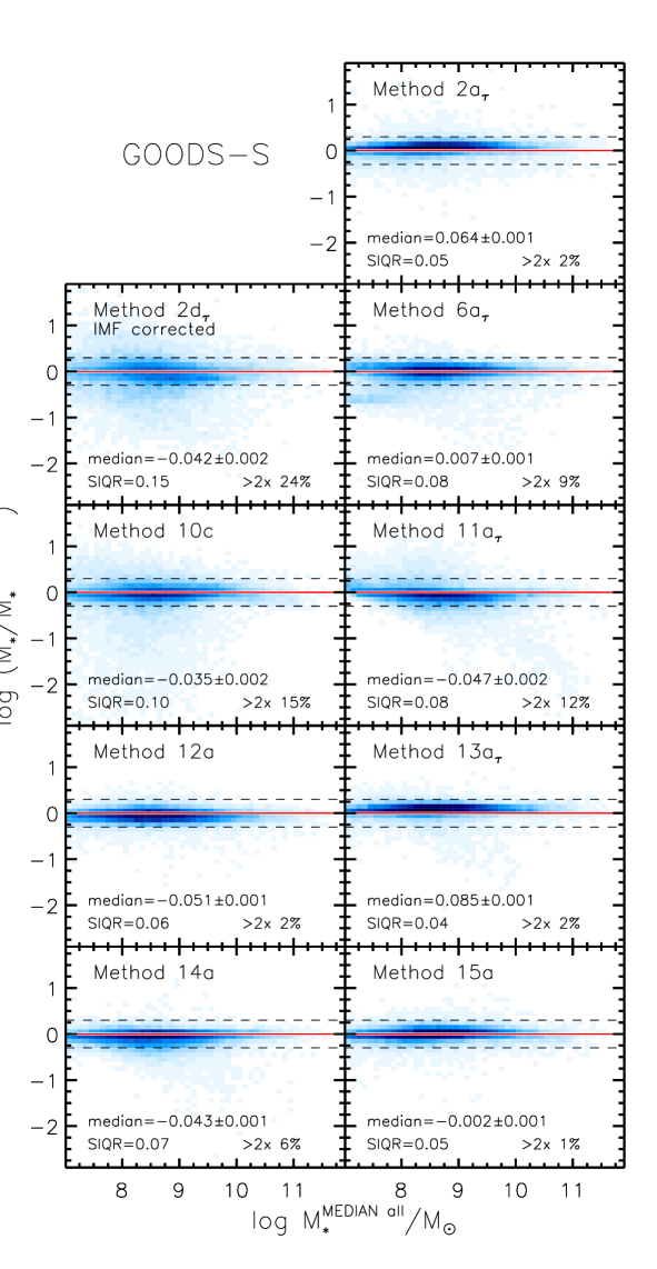
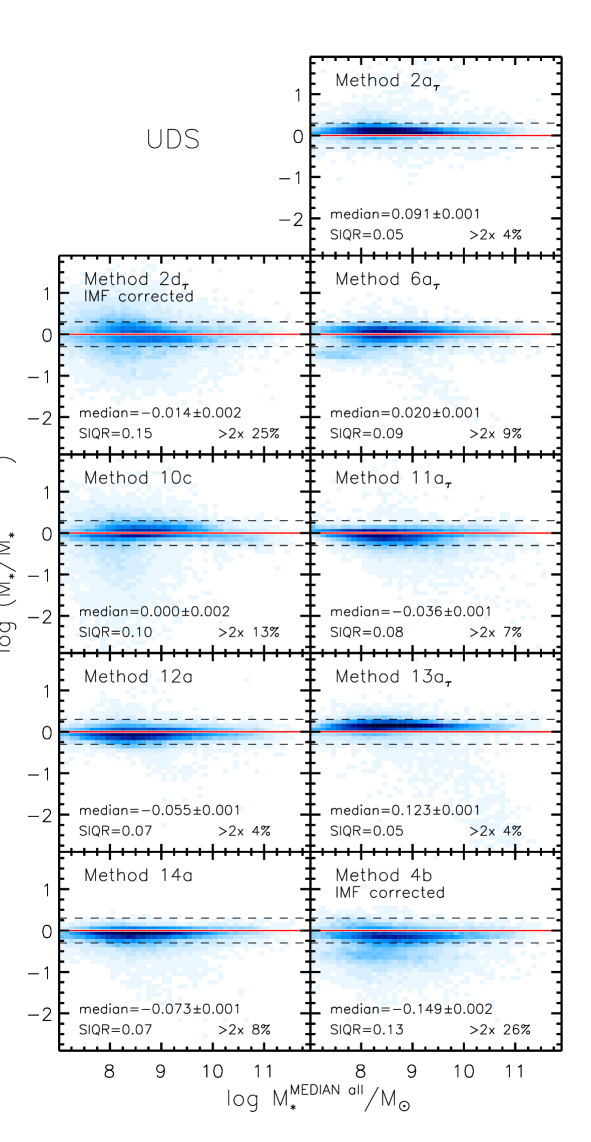
Figure 1.— Comparison between the ratio of the different stellar mass estimates and the median mass for the GOODS-S (left panels) and the UDS (right panels) samples. All masses have been rescaled to the same Chabrier IMF. The plane is colored according to the density of sources, increasing from lightest to darkest shades on a linear scale. The red solid horizontal line indicate null difference with respect to the median mass, while the black dashed lines enclose the region where the difference is within a factor of 2. The median logarithmic ratio with the associated error and the semi interquartile range (SIQR, see text) are printed in each panel, as well as the fraction of sources differing from the median value by more than a factor of 2 (i.e., falling beyond the dashed lines).

Figure 1 shows the ratio between each set of stellar masses and the median value as a function of the median. On average, the agreement among the different estimates is quite satisfactory, despite the different assumptions adopted. The uncertainty associated with the median value of the $\log(M_{*}/M_{*}^{\rm MEDIANall})$ distribution was computed as $\sigma/\sqrt{(2/\pi)N}$, where $\sigma$ is the standard deviation and $N$ is the number of objects one takes the median of, i.e., the number of galaxies in the sample. For most of the stellar mass sets, the majority of values are tightly clustered around the median of the distribution. We quantify the broadness of the distribution by means of the semi interquartile range (SIQR), defined as half the difference between the $75^{th}$ and the $25^{th}$ percentile. The typical SIQR is lower than 0.1 dex for most estimates. We also quantify the importance of the tails of the $\log(M_{*}/M_{*}^{\rm MEDIANall})$ distributions as the fraction of estimates differing from the median value by more than a factor of 2.

The stellar mass estimates showing the largest deviations from the median (SIQR$\sim$0.1-0.15) are those based on stellar templates other than BC03 (Methods 2d_τ, 4b and 10c). BC03 templates, adopted by most of the teams, strongly constrain the median value. The same methods also show the largest fraction of objects in the tails of the distribution (13–26%). Two teams (Methods 4b and 10c) have used stellar templates including a treatment of the TP-AGB phase (Maraston, 2005; Marigo et al., 2008). The enhanced emission at near-IR wavelengths due to the contribution of TP-AGB stars, especially for galaxies dominated by intermediate-age stellar populations ($\sim$1 Gyr), forces an overall lower normalization, hence slightly smaller stellar masses (e.g., Maraston et al. 2006; van der Wel et al. 2006; M15). However, the scatter is larger than the offset (see also Santini et al. 2012b for a comparison between BC03- and CB07-based results).

Methods 4b and 10c present other differences compared to the other teams. For example, Method 10c is the only one that does not include extinction in the templates. With the aim of verifying whether the lack of extinction could be responsible for the large dispersion, we estimated the stellar mass by using the very same assumption as Method 10c but allowing for dust extinction (see Method 10c^dust presented in Appendix B). The SIQR and the fraction of objects in the tails of the distribution are only very mildly reduced if not unchanged (SIQR $=$ 0.09 and 0.08 and 15% and 12% of sources differ by more than a factor of 2 in GOOODS-S and UDS, respectively). This implies that dust reddening alone cannot explain the large scatter around the median value.

Both Methods 4b and 10c assume different SFH shapes instead of simple $\tau$ models, adopted by 5 out of 10 teams. We will demonstrate in Section IV.2 that stellar masses are stable against different parameterizations of the SFH (at least those we could directly test). However, the tail of the $\log(M_{*}/M_{*}^{\rm MEDIANall})$ distribution towards lower values disappears for Method 10c when only galaxies best-fitted with direct-$\tau$ models are considered, and the fraction of sources differing from the median by more than a factor of 2 decreases to 8% and 11% in GOODS-S and UDS, respectively. Nevertheless, the SIQR is basically unchanged (0.09 and 0.11 dex in the two fields, respectively).

Method 4b shows a distribution with respect to the median value that is slightly bimodal. This is partly responsible for its broadness. This effect has already been reported by M15, who ascribe it to parameter degeneracy combined with the adoption of different stellar templates and SFH with respect to the majority of other mass estimates. The degeneracy seems to cause the best solution to fluctuate between either a population of lower mass galaxies (likely young and star-forming) or alternatively a population of higher mass ones, in agreement with the median values. Method 4b differs from most of the others also due to the inclusion of nebular emission. Although we will demonstrate in Section IV.3 that nebular emission strongly affects stellar masses in only a subset of sources, it may increase the degeneracy when combined with some peculiar SFH parameterizations, e.g., inverted-$\tau$ models used by Method 4b.

Finally, Methods 2d_τ and 4b are based on a different choice of the IMF. They were converted to a Chabrier IMF by multiplying the masses by a constant value (i.e., by subtracting 0.24 dex, see above), which is a good approximation. Indeed, the fact that the median value of $\log(M_{*}/M_{*}^{\rm MEDIANall})$ is close to zero for Method 2d_τ provides a further confirmation of the applicability of a constant shift. For Method 4b the median is instead shifted to lower values. This is likely a consequence of the effect of inclusion of TP-AGB stars and parameter degeneracy discussed above. Anyway, the bulk of the galaxies are located reasonably close to zero, once again confirming the validity of the IMF conversion.

IV.2. Star formation histories

To better investigate the effect of the assumed parameterization of the SFH, we take advantage of the additional mass estimates that were provided by several teams and that are presented in Appendix B. Because these results are based on the very same assumptions as the mass estimates presented above except for the SFH parameterization, they allow us to isolate its effect on the mass estimates by leaving the other assumptions unchanged.

Figure 2 shows a comparison between the stellar masses in the GOODS-S sample computed under the assumption of direct-$\tau$, inverted-$\tau$, delayed-$\tau$ models, linearly increasing and constant SFH. Stellar masses computed assuming such different SFH parameterizations show a very good agreement with respect to direct-$\tau$ models, with narrow distributions (SIQR$\leq$0.07 dex) and no obvious offsets nor trends with stellar mass nor with redshift. The only notable feature is a group of sources having $M_{*}^{\tau}$ (i.e., the mass based on direct-$\tau$ models) much larger (by up to an order of magnitude) than $M_{*}^{INV}$ (i.e., the mass based on inverted-$\tau$ models, upper panels of Figure 2): these are galaxies which are old and massive according to the exponentially decreasing model fit, and young and low-mass when fitted with an exponentially increasing model. Indeed, sources with $\log(M_{*}^{INV}/M_{*}^{\tau})<-0.3$ have an average reddening E(B-V)$\sim$0.5 as inferred from the fit with inverted-$\tau$ models, but E(B-V)$<$0.1 when direct-$\tau$ models are adopted. On the other hand, sources above this threshold show similar reddening in both fits. In any case, such discrepant sources represent only 10% of objects, the rest of the sample showing $\log(M_{*}^{INV}/M_{*}^{\tau})$ within a factor of 2.

Our results are in agreement with the previous work of Lee et al. (2010), who concluded that stellar masses are robust and on average unaffected by the choice of the SFH because of a combination of effects in the estimate of the galaxy star formation rates and ages. However, discrepant results were found by other groups (Maraston et al., 2010; Pforr et al., 2012), who reported an underestimation of the stellar mass when parameterizing the SFH as direct-$\tau$ models compared to the mass predicted by semi-analytical models. According to their analyses, the mismatch can be as much as 0.6 dex, with the exact value depending on stellar mass, redshift, and fitting setup.

Our analysis does not include SFHs with bursts. However, Moustakas et al. (2011) suggested that the adoption of smooth, dust-free exponentially declining SFHs changes the stellar masses obtained with bursty models (where bursts are added to direct-$\tau$ models) by no more than 0.1 dex on average, and by less than a factor of 2 for individual galaxies (see also Moustakas et al. 2013 and references therein).

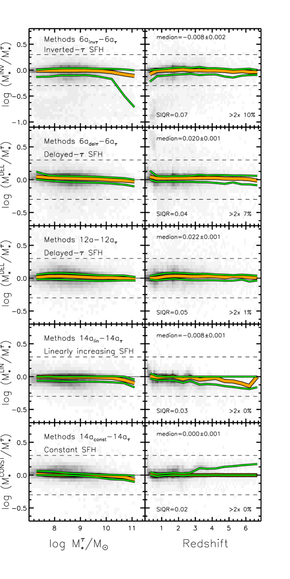
Figure 2.— Comparison among stellar masses computed with consistent methods except for the choice of the SFH for the GOODS-S field. The ratio between masses computed with direct-$\tau$ models ($M_{*}^{\tau}$), inverted-$\tau$ models ($M_{*}^{INV}$), delayed-$\tau$ models ($M_{*}^{DEL}$), linearly increasing models ($M_{*}^{LIN}$) and constant models ($M_{*}^{CONST}$) is studied against stellar mass ($M_{*}^{\tau}$, left panels) and redshift (right panels). Colors show density of sources as in Figure 1. The thick orange lines show the median in bins of mass ($\Delta\log M_{*}=0.5$) or redshift ($\Delta z=0.5$), while the two thin green lines enclose 50% of the sample (representing the 25${}^{t}h$ and 75${}^{t}h$ percentiles in the same bins). The median logarithmic ratio with the associated error and the semi interquartile range (SIQR, see text) are printed in each panel, as well as the fraction of sources differing from the median value by more than a factor of 2 (i.e., falling beyond the dashed lines). The black solid line shows the locus where the two stellar masses are comparable. Delayed-$\tau$ models in Method 6a_delτ have a slightly different analytic shape ($\psi(t)\propto t^{2}/\tau\cdot exp(-t/\tau)$) compared to Method 12a ($\psi(t)\propto t/\tau^{2}\cdot exp(-t/\tau)$).

IV.3. Nebular emission

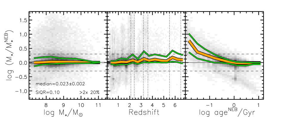
Figure 3.— Ratio between masses estimated without ($M_{*}$) and with ($M_{*}^{\rm NEB}$) nebular emission as a function of $M_{*}$ (left panel), redshift (central panel), and age as inferred from the fit including nebular contribution (age^NEB, right panel) for the GOODS-S field, using the estimates from Methods 6a_τ and 6a${}_{\tau}^{\rm NEB}$. Colors and line styles are as in Figure 2. Vertical dotted lines enclose three redshift ranges where strong nebular lines enter the near-IR filters, producing an overestimate of the stellar mass should they be ignored.

Only three teams (Methods 4b, 11a_τ and 14a) have included nebular emission in the stellar templates. However, because these three sets of stellar masses differ from the others also because of other assumptions, it is not an easy task to isolate the effect of nebular emission on the output stellar masses. For this reason, we take advantage from the results of Method 6a${}_{\tau}^{\rm NEB}$ presented in Appendix B, which differs from Method 6a_τ only due to the inclusion of nebular emission.

The comparison between stellar masses estimated without ($M_{*}$) and with ($M_{*}^{\rm NEB}$) nebular emission is shown in Figure 3. No significant offset is observed, nor are there trends as a function of stellar mass or redshift. Although the $\log M_{*}/M_{*}^{\rm NEB}$ distribution is very wide, the semi interquartile range is 0.1 dex, and 80% of the sample is confined within 0.3 dex from zero, meaning that the effect of nebular emission on wide band photometry is weak for the bulk of the population (see also G15). However, there are some exceptions that are worth discussing here.

The effect of nebular emission is slightly enhanced in particular redshift ranges, where strong nebular lines enter the near-IR filters, on which stellar mass is strongly dependent. Moreover, this effect is stronger at high redshift, where line emission contributes in a more effective way to the light in broad-band filters due to wavelength stretching as a consequence of cosmological expansion. The three redshift ranges where this effect is most evident are the $2.1<z<2.4$ region, where $J$, $H$ and $K$ band observe the [OII](3727Å), H$\beta$(4861Å) and [OIII](5007Å), and H$\alpha$(6563Å) lines, respectively, the $3.2<z<3.6$ region, where H$\beta$(4861Å) and [OIII](5007Å) lines enter the $K$ band and [OII](3727Å) line enters the $H$ band, and the $5.5<z<6.5$ region, where H$\beta$(4861Å) and [OIII](5007Å) lines are responsible for flux enhancement in the 3.6$\mu$m band. This is more clearly shown in Figure 4, where we plot the distribution of $\log M_{*}/M_{*}^{\rm NEB}$ in the $2.1<z<2.4$, $3.2<z<3.6$, and $5.5<z<6.5$ redshift windows compared to the distribution of the total sample. These redshift intervals show a positive tail in the distribution of $\log M_{*}/M_{*}^{\rm NEB}$ due to misinterpretation of nebular line emission as stellar continuum, resulting in a larger normalization in the best-fit template, hence in a larger stellar mass estimate. In summary, the overestimate of the stellar mass when ignoring nebular emission at high redshift, as predicted by previous works (e.g., Stark et al., 2013; Schenker et al., 2013), is enhanced in particular redshift ranges where strong lines enter the near-IR filters and does not affect most of the galaxy sample.

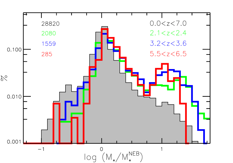
Figure 4.— Normalized distribution of the ratio between masses estimated without ($M_{*}$) and with ($M_{*}^{\rm NEB}$) nebular emission in the entire sample (shaded histogram) and in the $2.1<z<2.4$ (green histogram), $3.2<z<3.6$ (blue) and $5.5<z<6.5$ (red) redshift ranges, for the GOODS-S sample and using the estimates from Methods 6a_τ and 6a${}_{\tau}^{\rm NEB}$. The numbers in the upper left corner show the number of galaxies in each sample, with the same color-code.

In addition, although $\log M_{*}/M_{*}^{\rm NEB}$ is on average distributed around zero for the bulk of the population, its overall distribution is asymmetric, with a tail towards higher values (see shaded histogram in Figure 4). Because the spectra of young and star-forming galaxies are characterized by many (and intense) nebular emission lines, we expect that the effect of including or neglecting nebular emission may depend on the galaxy age. In fact, a well defined trend of $\log M_{*}/M_{*}^{\rm NEB}$ can be observed as a function of age as inferred from the fit including the nebular contribution (age^NEB, right panel of Figure 3): stellar masses turn out to be severely overestimated (by as much as an order of magnitude) in young (age^NEB$<$100 Myr) galaxies if nebular emission is ignored. Indeed, strong nebular lines in their spectra may mimic the Balmer and 4000Å breaks, resulting in these sources being fitted better by older, passive, and more massive templates (see also Atek et al., 2011). To further explore this effect, we plot in Figure 5 the ratio between stellar masses ($\log M_{*}/M_{*}^{\rm NEB}$) as a function of the ratio of ages ($\log{\rm age}^{\rm NEB}/{\rm age}$), and color-code symbols according to the ratio of their SFRs ($\log{\rm SFR}^{\rm NEB}/{\rm SFR}$), where the superscript NEB denotes the parameters inferred from the fit with templates including nebular emission. The stellar mass ratio is strongly correlated with the age ratio as well as with the SFR ratio. As noted above, ignoring nebular emission produces an overestimate of the stellar mass in galaxies that are young and star-forming according to the fit with nebular emission, while the stellar mass is mostly unaffected when the best-fit age and SFR computed with and without the nebular contribution are consistent. In general, when comparing two distinct estimates of the stellar mass, the largest differences are observed in galaxies that have a young star-forming solution in one fit and an old passive solution in the other, as shown in Figure 5. This behavior is common to every pair of fits and not specific to the case with/without nebular emission, as also discussed by M15.

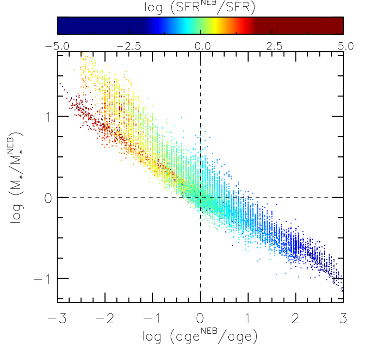
Figure 5.— Ratio between masses estimated without ($M_{*}$) and with ($M_{*}^{\rm NEB}$) nebular emission as a function of the ratio between ages as inferred from the fit with (${\rm age}^{\rm NEB}$) and without (age) nebular emission, for the GOODS-S field and using the estimates from Methods 6a_τ and 6a${}_{\tau}^{\rm NEB}$. Symbols are color-coded according to the ratio of their SFRs.

Finally, in order to understand how important is the particular implementation of nebular emission compared to including it at all, we compared the results of the four methods that include the nebular component, i.e., Methods 4b, 6a${}_{\tau}^{\rm NEB}$, 11a_τ and 14a. More specifically, we compared each method with the median of the four, in a similar way as done in Figure 1, after rescaling all masses to the same Chabrier IMF. The methods accounting for nebular emission generally agree with each other better than they do with the methods not including it: the distributions of the ratio between each of the methods and their median has a SIQR of 0.05–0.1 dex, with a fraction of $<15\%$ of sources differing by more than a factor of 2. The only exception is Method 4b. However, we ascribe its wider distribution to the different stellar isochrone models adopted by this method, as discussed in Section IV.1.

To summarize, Figures 3, 4, and 5 show that 80% of the population is unaffected by the inclusion of nebular emission (see also G15), and $\log M_{*}/M_{*}^{\rm NEB}$ is consistent with 0. For these galaxies, the inclusion of nebular emission does not change the stellar mass by more than a factor of 2. However, nebular emission can strongly affect the light emitted by subclasses of galaxies, notably galaxies in particular redshift ranges (especially at $z>3$) or young (${\rm age}^{\rm NEB}<100$Myr) sources. For extremely young (${\rm age}^{\rm NEB}\lesssim 20$Myr) galaxies, ignoring nebular emission may produce an overestimate of the stellar mass by more than a factor of 10. The sources whose difference in the stellar mass is larger than a factor of 6 (i.e., beyond the minimum shown by the histograms in Figure 4) is 6% of the total sample.

V. CANDELS reference stellar masses

V.1. The median mass approach

Given the results shown in the previous sections, we can conclude that the stellar mass is a stable parameter against different assumptions in the fit for the majority of the galaxy population. Except for the IMF, which introduces a roughly constant offset, the most important assumption is the choice of the stellar population synthesis templates (see also M15), which seem to severely affect stellar mass estimates. Because BC03 templates are assumed by most of the teams (7 out of 9 for the GOODS-S sample, 6 out of 9 for the UDS sample), we decided to compute a median mass by only considering BC03-based estimates: in the GOODS-S field we consider stellar masses from Methods 2a_τ, 6a_τ, 11a_τ, 12a, 13a_τ, 14a, 15a, while in the UDS field we consider masses from Methods 2a_τ, 6a_τ, 11a_τ, 12a, 13a_τ, 14a. As demonstrated by M15, the median value provides the most accurate measure of the stellar mass, as long as the individual estimates are unbiased compared to each other, as is the case (see previous Section).

Because only a limited number of measurements are available, we adopted the Hodges-Lehmann estimator (see Equation 1) instead of the median, as explained in Section IV.1, computed in linear space. We refer to this median value as $M_{*}^{\rm\rm MEDIAN}$ and consider it the reference mass for the CANDELS catalogs.

We quantify the scatter around the median value caused by the different assumptions for computing stellar masses by means of the standard deviation ($\sigma_{M,{\rm CANDELS}}$) of the various methods, again computed in linear space and only considering the methods adopting BC03 stellar templates. Therefore, this scatter does not, by definition, account for the effect of stellar evolution modeling, such as for example the inclusion of the TP-AGB phase, but it is mainly caused by differences in the technicalities in the mass computation, in the parameter grid sampling, in the assumed SFH, and in the prior assumptions. This scatter is roughly 25-35% of the median values and shows no trend with age nor with rest-frame colors.

Figure 6 shows CANDELS reference stellar masses as a function of observed $H_{160}$ band magnitude, while Figure 7 shows them as a function of redshift, in GOODS-S and UDS. The right panels of both figures show a comparison between the two fields. In Figure 7 we cut both samples to $H_{160}<26.5$ to account for different observational depth in the two fields. The $M_{*}$–$H_{160}$ and $M_{*}$–$z$ relations agree very well in the two fields, confirming the consistency of the photometry, i.e., meaning that there are no issues associated with colors or photometric redshifts.

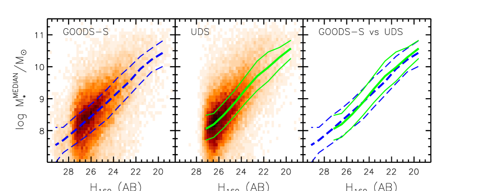
Figure 6.— Reference median stellar mass (see Section V.1) as a function of the observed $H_{160}$ band magnitude in GOODS-S (left panel) and UDS (central panel). The color reflects the density of sources, increasing from lightest to darkest on a linear scale. Thick lines show the median mass in bins of one magnitude, while thin lines show the semi interquartile range in the same bins. Medians and semi interquartile ranges are also reported in the right panel for a direct comparison between the two fields (GOODS-S: blue dashed; UDS: green solid).

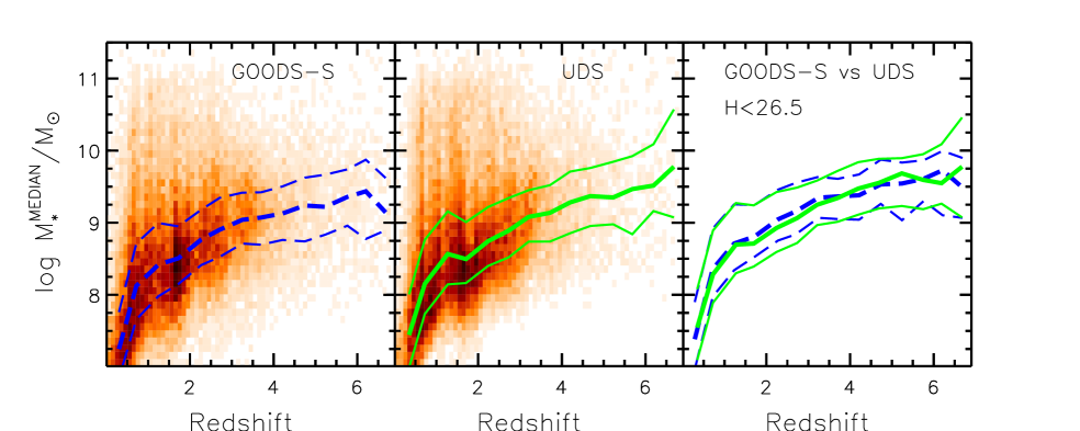
Figure 7.— Reference median stellar mass (see Section V.1) as a function of redshift in GOODS-S (left panel) and UDS (central panel). Colors and line styles are as in Figure 6. Thick lines show the median mass in bins of redshift ($\Delta z=0.5$), while thin lines show the semi interquartile range in the same bins. The right panel shows medians and semi interquartile ranges for the two samples cut at $H_{160}<26.5$.

V.2. Overall scatter among different methods vs scatter due to model degeneracy and photo-$z$ uncertainty

All the stellar mass estimates that we are considering and comparing in the present work are computed by assuming the photometric or spectroscopic redshift at their reported value, not accounting any redshift uncertainties. However, as shown by G15 when measuring galaxy stellar mass functions, the reliability of photometric redshift may represent the major source of uncertainty in the stellar mass estimate. Moreover, the effect of model degeneracy (i.e., the possibility of having two or more different SEDs fitting the observations equally well because of the similar effects on broad-band colors due to varying SFH, age, metallicity, dust) may be significant and should not be underestimated. This effect is reflected by the width of the probability distribution function PDF($M_{*}$).

We estimate here the relative uncertainty on the stellar mass originating from the scatter in the photometric redshifts combined with model degeneracy and compare it with the systematic uncertainty caused by adoption of different assumptions (but the same redshifts) from the various teams. We quantify relative uncertainties as $\delta_{\rm M}=\sigma/M_{*}$, where $\sigma$ is the standard deviation of the mass distribution for each object.

The relative uncertainty in the stellar mass estimates caused by different assumptions in the fit is indicated as $\delta_{M,{\rm CANDELS}}=\sigma_{M,{\rm CANDELS}}/M_{*}^{\rm MEDIAN}$. For each object, $\sigma_{M,{\rm CANDELS}}$ was calculated as explained in the previous Section.

The relative uncertainty derived from model degeneracy and uncertainties in the photometric redshift determination, denoted by $\delta_{M,z}=\sigma_{M,z}/M_{*M,z}$, depends on the width of the redshift probability distributions function PDF($z$) (D13) and on photometric errors. It was estimated by means of a Monte Carlo simulation as explained by G15. Briefly, for each galaxy lacking a spectroscopic estimate, a random redshift was extracted according to its PDF($z$), and a PDF($M_{*}$) was computed by fitting the observed photometry at the extracted redshift following Method 6a_τ. For spectroscopic sources, a single PDF($M_{*}$) was calculated by fixing the redshift to its spectroscopic value. A mass estimate was then extracted according to the PDF($M_{*}$). This procedure was repeated 10000 times for each object and a standard deviation ($\sigma_{M,z}$) and a mean value ($M_{*M,z}$) of the resulting mass distribution were computed in linear space. $\delta_{M,z}$ is included in the released mass catalogs.

Figure 8 shows the ratio between the relative uncertainty due to model degeneracy and photometric redshifts scatter ($\delta_{M,z}$) and that due to differing assumptions in the SED fitting ($\delta_{M,{\rm CANDELS}}$), as a function of stellar mass and redshift. $\delta_{M,z}$ is on average larger than $\delta_{M,{\rm CANDELS}}$, at least for the bulk of the population, by a factor of $\sim$2. This factor increases for low-mass sources and is close to unity at high stellar masses. Indeed, massive galaxies have more accurate photometry thanks to the higher S/N, hence have more accurate photometric redshifts and allow a lower level of model degeneracy in the fit. No trend is observed with redshift.

The fact that the uncertainty due to the assumptions in the fit is on average smaller than that originating from models degeneracy and photo-$z$ scatter further justifies our choice of computing the median of estimates performed by the various teams, despite the different assumptions (see Table 1).

It is interesting to compare the value of $\delta_{M,z}$ in spectroscopic and photometric sources, in order to have an idea of the contribution of photometric redshift scatter compared to model degeneracy. The average $\delta_{M,z}$ is about two times larger for sources lacking good quality spectra compared to spectroscopic galaxies. Photometric redshifts scatter therefore makes the uncertainty in stellar masses worse by a factor of 2, compared to what inevitably one gets due to model degeneracy. However, the spectroscopic sample is biased toward the brightest galaxies, which have the cleanest photometry and therefore suffer from the lowest level of model degeneracy in the fit. Fainter galaxies are susceptible to a higher degeneracy.

In conclusion, Figure 8 illustrates that model degeneracy and photometric redshift scatter remain the largest source of uncertainty when estimating stellar masses: the relative mass uncertainty due to model degeneracy and photo-$z$ exceeds that due to other systematics (assumptions and details in the fits and choice of the parameters grid) by a factor of 2 for the bulk of the population, and potentially by factors of  several toward lower masses. Only for the most massive galaxies is the contribution of model degeneracy associated with photo-$z$ scatter comparable to that of systematics in the mass computation.

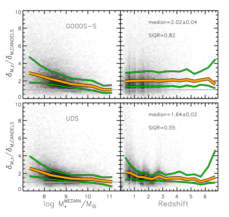
Figure 8.— Ratio between the relative uncertainty caused by model degeneracy and scatter in the photometric redshifts ($\delta_{M,z}$) and that due to the adoption of different assumptions in the SED fitting ($\delta_{M,{\rm CANDELS}}$), as a function of the reference median mass (left panels) and redshift (right panels). Upper and lower panels show the GOODS-S and UDS samples, respectively. Colors and line styles are as in Figure 2. The black horizontal line shows the locus where the two uncertainties are comparable.

V.3. Comparison with 3D-HST stellar masses

We compare CANDELS reference stellar masses with those released by the 3D-HST team for the same fields (Skelton et al., 2014), by matching the two catalogs in position with a tolerance of 0.1 arcsec. They use BC03 templates, assume a Chabrier IMF, direct-$\tau$ model SFHs with a minimum timescale $\log(\tau/yr)$ of 7, Solar metallicity, a minimum $\log({\rm age}/yr)=7.6$, a Calzetti extinction law with 0.0$<$E(B-V)$<$1.0, and do not include nebular emission. Because their masses are computed on different photometric catalogs and hence assuming different photometric redshifts, we only consider those sources whose redshifts differ by less than 0.1. The requirement that positions and redshifts are within the tolerance leaves us with $\sim 40\%$ of the CANDELS sample. The comparison, as a function of both CANDELS median masses and redshifts, is shown in Figure 9.

The comparison is satisfying at a first-order glance, with quite narrow dispersion (SIQR $\sim 0.1$ dex), increasing towards high redshifts, where sources are generally fainter and photometry is noisier. However, a slight negative median offset ($\sim$$-0.1$ dex) in both fields and a curved trend in UDS are observed. These effects could be ascribed to systematics in the SED fitting, in particular affecting 3D-HST results. Indeed, while 3D-HST stellar masses result from a single fit, CANDELS stellar masses are computed with a median approach, which is able to wash out systematic biases affecting specific assumptions in the SED modelling and was demonstrated to provide a more robust measure (M15). To check whether this may be the cause, we compare 3D-HST masses with the mass estimate within CANDELS whose method and assumptions are closest 3D-HST ones, i.e. Method 2a_τ. The offset is reduced (median $=0.010\pm 0.003$ in GOODS-S and median $=-0.060\pm 0.002$ in UDS), but the curved trend is mostly unchanged. The residual offset observed in the UDS field and the curved trend may be due to systematics in the photometry. Indeed, UDS, having data of poorer quality, might be more susceptible to biases compared to the better quality data in GOODS-S.

The difference between CANDELS and 3D-HST stellar mass estimates (SIQR $\sim 0.1$ dex) is only slightly larger than the typical dispersion observed among different estimates within CANDELS assuming the same stellar models. However, the distributions are overall more extended: the fraction of objects differing by more than a factor of 2 is 11% and 15% in GOODS-S and UDS, respectively. If the distributions are shifted so that the average offset is zero, these fractions are marginally reduced (10%). They are equal to 12% and 11% if 3D-HST masses are compared to Method 2a_τ instead of the median CANDELS masses, reflecting an intrinsic larger distribution due to differences in the photometry and in the redshifts in addition to the systematics in the mass estimates.

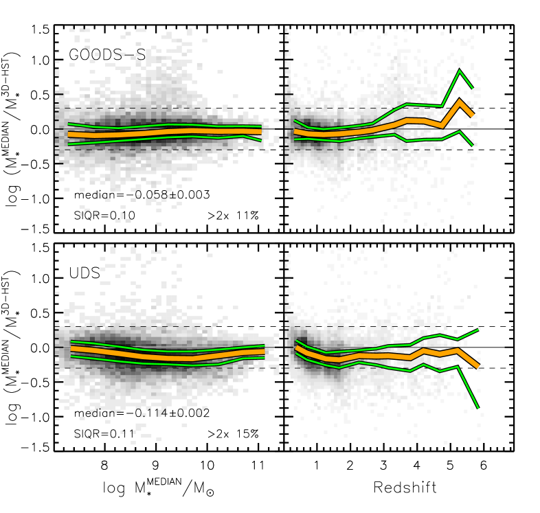
Figure 9.— Ratio between CANDELS median masses and 3D-HST masses as a function of CANDELS median masses (left panels) and CANDELS redshifts (right panels) for the GOODS-S field (upper panels) and the UDS fields (lower panels). Only sources whose redshifts differ by less than 0.1 have been considered. Colors and line styles are as in Figure 2.

V.4. CANDELS stellar mass catalogs

The median approach has revealed a powerful tool to overcome systematics associated with the choice of the SED fitting parameters (see previous section and M15). For this reason, the catalogs presented here include the CANDELS reference median mass ($M_{*}^{\rm MEDIAN}$) as well as the median of only the methods including nebular emission (and based on the same stellar isochrone library, i.e., Methods 6a${}_{\tau}^{NEB}$, 11a_τ and 14a), in both cases with their associated scatters (see Section V.1). Nevertheless, the catalogs also contain each individual estimate of the stellar mass for each source (Tables 1 and 4). The various sets of stellar mass measurements agree on average, at least those based on the same stellar templates. However, the different assumptions, such as the SFH parameterization or the inclusion of nebular emission, may produce very different results for few peculiar and interesting objects or for subsets of very young galaxies (see for example Figure 3). The comparison of the various methods may then provide interesting information and a deeper insight in the galaxy evolution paradigm.

In addition to the stellar masses, we also include in a separate file other physical parameters (such as age, SFR, metallicity, dust reddening, etc) and rest-frame magnitudes as estimated from the various methods. The same file also incorporates the uncertainties in the stellar masses, neglecting redshift errors, associated with methods 6a_τ, 11a_τ and 12a.

Both files for each field are released as electronic tables in the online version of the Journal and are uploaded on the STScI MAST archive website for CANDELS. Tables showing the list of columns in each catalog are reported in Appendix C. The catalogs are also available in the Rainbow Database (Pérez-González et al., 2008; Barro et al., 2011a), which features a query menu that allows users to search for individual galaxies, create subsets of the complete sample based on different criteria, and inspect cutouts of the galaxies in any of the available bands. It also includes a crossmatching tool to compare against user uploaded catalogs.

VI. Summary

This paper accompanies the public release of the CANDELS mass catalogs for the GOODS-S and UDS fields. We present and make publicly available the reference CANDELS stellar masses obtained by combining the results from various teams within the collaboration. Masses are estimated adopting the official CANDELS photometry and assuming spectroscopic redshifts when available, or the official CANDELS photometric redshifts (Dahlen et al. in prep.) otherwise. We also release the individual stellar mass estimates computed by each team, as their comparison may be useful especially when studying peculiar objects, as well as other physical parameters (such as age, SFR, metallicity, dust reddening, etc) and rest-frame magnitudes associated with the SED fitting.

The availability of several mass estimates has allowed us to compare methods, from which we conclude the following:

• The results from the various teams are in overall good agreement despite the different methods, assumptions, and priors.

• The parameter which has the greatest effect on the stellar mass is the stellar isochrone library: due to different modeling of several stellar evolutionary phases, such as the TP-AGB phase, the adoption of different libraries produces a dispersion (in terms of the semi interquartile range) larger than 0.1 dex, while the dispersion shown by estimates based on the same stellar templates is on average smaller.

• Stellar masses are stable against the choice of the SFH parameterization and differences in the metallicity/extinction/age parameter grid sampling.

• The IMF only affects stellar masses as an overall scaling, as expected.

• The inclusion of nebular emission can have a large effect but only on a small fraction of the sample. Specifically, ignoring nebular emission in the model spectra may cause an overestimate of the stellar mass in galaxies that are either young ($<100$Myr) or lie in particular redshift ranges, especially at high redshift. Indeed, in these redshift windows strong nebular lines enter the near-IR filters, on which stellar mass is strongly dependent. The overestimate can exceed a factor of 10 in extremely young ($<20$Myr) galaxies. Nevertheless, the effect of nebular emission is negligible for the majority (80%) of galaxies. As current and future surveys push observations towards the youngest Universe, it becomes crucial to investigate whether the assumptions adopted to include nebular emission in the models are correct, in order to infer the most reliable stellar masses for the first galaxies.

Based on these results, we combined all mass estimates assuming the same stellar templates and IMF by means of the Hodges-Lehmann estimator. The standard deviation among different methods is a measure of the systematic uncertainties affecting stellar masses due to the choice of the assumptions and priors adopted in the fit and parameter grid sampling. Such systematics are smaller, by a factor of 2 on average, than the uncertainty due to model degeneracy and scatter in photometric redshifts. Among these, the latter dominate over model degeneracy. However, this can only be tested in sources with robust, spectroscopic redshifts, and at the same time model degeneracies are expected to become more important for faint galaxies (lacking spectroscopic observations) due to the larger photometric errors.

Finally, we compare CANDELS stellar masses with those released by the 3D-HST team. The agreement is satisfying at a first-order glance, but we observe a negative median offset ($\sim$-0.1dex) in both fields and a curved trend in UDS. The offset disappears in GOODS-S and is reduced in UDS when 3D-HST results are compared with the method adopting the closest assumptions to the 3D-HST team. While we cannot say whether or not any one technique is biased, our tests with mock catalogs in M15 suggests that the median mass is less susceptible to modeling uncertainties than the results from any one code. The different behavior of GOODS-S and UDS in the comparison to 3D-HST also illustrates that differences in photometric quality (number of filters and S/N) can affect not only the scatter but also the biases between methods (the poorer quality dataset available in UDS compared to the more accurate photometry in GOODS-S is more susceptible to biases). In any case, we show that the larger fraction of objects in the tails of the $\log(M_{*}^{\rm MEDIAN}/M_{*}^{\rm 3D-HST})$ distributions are at least partially explained by differences in the photometric and redshift catalogs.

Appendix A Magellan/IMACS spectroscopy in UDS

As first discussed in Section II.2, our analysis and stellar mass catalog for the UDS field includes redshift measurements derived from spectroscopic observations in the CANDELS/UDS field using the Inamori-Magellan Areal Camera and Spectrograph (IMACS, Dressler et al., 2011) on the Magellan Baade 6.5-meter telescope. The Magellan/IMACS spectroscopic sample includes a total of $475$ unique sources, spread over $4$ slitmasks and covering an area slightly larger than the CANDELS HST/WFC3-IR footprint in the UDS. The observations were conducted on the nights of December 30-31, 2010 (UT), with total exposure time of roughly $5400$ seconds per slitmask ($3~{}\times~{}1800$ s with no dithering performed). Immediately following each set of science exposures (i.e., without moving the telescope or modifying the instrument configuration), a quartz flat-field frame and comparison arc spectrum (using He, Ar, Ne) were taken to account for instrument flexure and detector fringing. Each slitmask contains on the order of 125 slitlets, with a fixed slitlength and slitwidth of $8^{\prime\prime}$ and $1^{\prime\prime}$, respectively. We employed the 300 lines/mm grism (${\rm blaze~{}angle}=26.7^{\circ}$) with the clear (or ”spectroscopic”) filter, which yields a spectral resolution of $R\sim 1200$ at $7500$Å.

The $475$ unique sources in the Magellan/IMACS spectroscopic sample are drawn from the Subaru optical imaging catalog of Furusawa et al. (2008), which covers the larger $1.22~{}{\rm degree}^{2}$ Subaru/XMM-Newton Deep Survey (SXDS, Ueda et al., 2008) field surrounding the CANDELS/UDS region. We identified spectroscopic targets according to an $R_{c}$ band limiting magnitude of $R_{c}<23.5$ (AB), with sources brighter than $R_{c}=18$ excluded from the target population. In an effort to primarily observe galaxies at intermediate redshift, we prioritized targets according to a $BR_{c}i^{\prime}$ color selection, closely mirroring that of the DEEP2 Galaxy Redshift Survey (Davis et al., 2003, 2007; Newman et al., 2013). The color-cut, as shown in Figure 10, is defined using a large pool of publicly-available redshifts covering the wider SXDS field (Simpson et al., 2006; Geach et al., 2007; van Breukelen et al., 2007; Smail et al., 2008) and corresponds to the following selection criteria:

$$(B-R_{c}) <0.5~{}{\rm or}$$ (A1)

$$(R_{c}-I) >0.85~{}{\rm or}$$ (A2)

$$(B-R_{c}) <2.3\bar{3}\times(R_{c}-I)-0.08\bar{3}.$$ (A3)

Objects failing these color selection criteria are included in the sample, but with a lower probability of inclusion in the target population. In addition, we downweighted those objects with SExtractor stellarity index of ${\rm CLASS\_STAR}>0.95$ (i.e., stars, Bertin & Arnouts, 1996).

The IMACS spectroscopic observations were reduced using the COSMOS data reduction pipeline developed at the Carnegie Observatories (Dressler et al., 2011). For each slitlet, COSMOS yields a flat-fielded and sky-subtracted, two-dimensional spectrum, with wavelength calibration performed by fitting to the arc lamp emission lines. One-dimensional spectra were extracted and redshifts were measured from the reduced spectra using additional software developed as part of the DEEP2 and DEEP3 Galaxy Redshift Surveys (Newman et al., 2013; Cooper et al., 2011, 2012c) and adapted for use with IMACS as part of the Arizona CDFS Environment Survey (Cooper et al., 2012b) and as part of the spectroscopic follow-up of the Red-Sequence Cluster Survey (RCS Gladders & Yee, 2005, zRCS; Yan et al. in preparation). A detailed description of the DEEP2 reduction packages (SPEC2D and SPEC1D) is presented by Cooper et al. (2012a) and Newman et al. (2013).

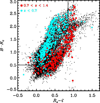
Figure 10.— The $B-R_{c}$ versus $R_{c}-I$ color-color distribution for all sources with $R_{c}<23.5$ in the Subaru imaging catalogs of Furusawa et al. (2008). The cyan and red points correspond to those objects with spectroscopic redshifts in the ranges $z<0.7$ and $0.7<z<1.4$, respectively. The solid black lines show the color cuts employed to prioritize target selection (see Equation A3).

Figure 11.— The distribution of the 352 unique, secure ($Q=-1$, $3$, $4$) redshifts included in the Magellan/IMACS redshift catalog.

All spectra were visually inspected by M. Cooper, with a quality code ($Q$) assigned corresponding to the accuracy of the redshift value — $Q=-1,3,4$ denote secure redshifts, with $Q=-1$ corresponding to stellar sources and $Q=3,4$ denoting secure galaxy redshifts (see Table 3). Confirmation of multiple spectral features was generally required to assign a quality code of $Q=3$ or $4$. Quality codes of $Q=1$, $2$ were assigned to observations that yield no useful redshift information ($Q=1$) or may possibly yield redshift information after further analysis or re-reduction of the data ($Q=2$). For detailed descriptions of the reduction pipeline, redshift measurement code, and quality assignment process refer to Wirth et al. (2004), Davis et al. (2007), and Newman et al. (2013). A redshift catalog is presented in Table 3, a subset of which is listed herein. The entirety of Table 3 appears in the electronic version of the Journal. A redshift is only included when classified as secure ($Q=-1,3,4$). The total number of secure redshifts in the sample is $352$ out of $475$ total, unique targets. The redshift distribution for this sample, as shown in Figure 11, peaks at $z<1$ with a small tail out to higher redshift. Across the $4$ slitmasks, a total of $44$ objects in the Magellan/IMACS sample were observed more than once. While not a large sample of repeated observations, these independent spectra provide a direct means for determining the precision of the redshift measurements. A comparison of the differences in the redshift measurements for multiple observations of the same object yields a redshift precision of $\sigma_{z}\sim 30~{}{\rm km}~{}{\rm s}^{-1}$ (for $Q=-1$, $3$, and $4$).

Table 3 Magellan/IMACS Redshift Catalog

Object ID	$\alpha$ (J2000)	$\delta$ (J2000)	$R_{c}$	Mask	Slit	MJD	$z$	$z_{\rm helio}$	$Q$
30007451	34.212042	-5.206258	21.85	UDS1	1	55560.6	0.80924	0.80915	4
30008565	34.215329	-5.214261	22.57	UDS1	2	55560.6	0.81222	0.81213	4
30009829	34.219258	-5.242188	22.84	UDS1	3	55560.6	0.92968	0.92960	3
30011686	34.226008	-5.258772	22.15	UDS1	4	55560.6	0.80341	0.80332	4

Note. — Table 3 is presented in its entirety in the electronic edition of the Journal. A portion is shown here for guidance regarding its form and content.

Appendix B Additional stellar mass estimates

In addition to the mass estimates presented in Table 1, several teams have provided further results based on different assumptions, which we present in Table 4. We excluded these estimates from the median computation in order not to overweight a single method compared to the others. However, we used them to test how specific parameters affect the best-fit result. Indeed, the methods listed in Table 4 offer the advantage of being based on the very same assumption as their analogues in Table 1 except for a single parameter. This makes it possible to study the effect of such parameter on the output stellar mass by leaving the other assumptions unchanged.

We list below the differences between the methods presented in Table 4 and those in Table 1.

• Method 6a${}_{\tau}^{\rm NEB}$ is completely consistent with Method 6a_τ except for inclusion of nebular emission. Nebular emission is treated following Schaerer & de Barros (2009), as already presented by Castellano et al. (2014) and by G15, in a very similar way as Method 14a. Briefly, Schaerer & de Barros (2009) directly link nebular emission to the amount of hydrogen-ionizing photons in the stellar spectra (Schaerer & Vacca, 1998) by considering free-free, free-bound, and hydrogen two-photon continuum emission. They assume null escape fraction, an electron temperature of $10^{4}$ K, an electron density $N_{e}$=100 cm⁻³, and a 10% helium numerical abundance relative to hydrogen. Hydrogen lines from the Lyman to the Brackett series were included considering Case B recombination, while the relative line intensities of He and metals depend on the metallicity according to Anders & Fritze-v. Alvensleben (2003). We refer the reader to the works above for more details.

• Methods 6a_delτ and 6a_invτ are completely consistent with Method 6a_τ except for the SFH: delayed-$\tau$ and inverted-$\tau$ models have been used, respectively, instead of direct-$\tau$ models. Delayed-$\tau$ models have a slightly different analytic shape ($\psi(t)\propto t^{2}/\tau\cdot exp(-t/\tau)$) compared to Methods 12a, 14a, and 15a presented in Table 1 ($\psi(t)\propto t/\tau^{2}\cdot exp(-t/\tau)$).

• Method 10c^dust is completely consistent with Method 10c, but dust reddening has now been included according to a Calzetti attenuation law.

• Method 12a_τ is consistent with Method 12a except for the SFH parameterization (direct-$\tau$ models instead of delayed-$\tau$).

Moreover, to analyze the effect of the SFH modeling on the mass estimates, we also take advantage from the results of Method 14a. In addition to the best-fit results (which we refer to as Method 14a), this method provides the full set of physical parameters for each of the four SFH model adopted: constant (Method 14a_const), linearly increasing (Method 14a_lin), delayed-$\tau$ (Method 14a_delτ), and direct-$\tau$ models (Method 14a_τ).

Table 4 Additional stellar masses in CANDELS (not considered for the median computation).

	Method 6a${}_{\tau}^{\rm NEB}$	Method 6adelτ	Method 6ainvτ	Method 10cdust	Method 12aτ
PI	A. Fontana	A. Fontana	A. Fontana	J. Pforr	T. Wiklind
fitting method	min $\chi^{2}$	min $\chi^{2}$	min $\chi^{2}$	min $\chi^{2}$	min $\chi^{2}$
code	zphot	zphota	zphota	HyperZ	WikZ
stellar templates	BC03	BC03d	BC03d	BC03d	M05
IMF	Chabrier	Chabrier	Chabrier	Chabrier	Chabrier
SFH	$\tau$	del-$\tau$	inv-$\tau$	$\tau$f + trunc. + const.	$\tau$f
log ($\tau$/yr)	8.0–10.2	8.0–9.3	8.0–10.2	8.5, 9.0, 10.0	-$\infty$ – 9.0
steps	9 steps	20 steps	9 steps		8 steps
log ($t_{0}$/yr)				8.0, 8.5, 9.0
metallicity [Z⊙]	0.02, 0.2, 1, 2.5	0.02, 0.2, 1, 2.5	0.02, 0.2, 1, 2.5	0.2, 0.5, 1, 2.5	0.2, 0.4, 1, 2.5
log (age/yr)	7.0–10.1	7.0–10.1	7.0–10.1	8.0–10.3	7.7–9.8
stepsl	110 steps	113 steps	48 steps	221 steps	24 steps
extinction law	Calzetti + SMC	Calzetti + SMC	Calzetti + SMC	Calzetti	Calzetti
extinction E(B-V)	0.0–1.1	0.0–1.1	0.0–1.1	0.00–0.75	0.0–1.0
step	0.05	0.05	0.05	0.05	0.025
nebular emission	yes	no	no	no	no
priors		n o	n o	n	n
reference	4	4	4	5	7

Note. — References. (4) Fontana et al. (2006); (5) Daddi et al. (2005); Maraston et al. (2006); Pforr et al. (2012, 2013); (7) Wiklind et al. (2008, 2014).

Appendix C Notes on the released catalogs

We report in Tables 5 and 6 the list of columns in the mass catalogs and in the catalogs containing the other physical parameters, respectively. Fig.12 shows the filter curves over which rest-frame magnitudes have been computed following Methods 6a_τ, 6a${}_{\tau}^{\rm NEB}$, 6a_delτ and 6a_invτ (see Table 6). Filter curves are available as ascii files in the electronic version of the Journal.

Table 5 List of columns in the mass catalogs for the GOODS-S (filename GS_CANDELS_mass.dat) and UDS (filename UDS_CANDELS_mass.dat) fields.

# column	# column	Description	Notes
GOODS-S	UDS
1	1	Designation
2	2	RA	J2000
3	3	Dec	J2000
4	4	Observed magnitude in the F160W filter
5	5	Signal-to-noise ratio in the F160W filter
6	6	Photometry flag	0: ok; $>$0: bad photometry
7	7	Spectroscopic star flag	?$=$1 spectroscopic star
8	8	Stellarity index from Sextractor on F160W band
9	9	AGN flag	?$=$1 Xray AGN
10	10	Redshift best estimate	see catalogs’ readme file for details
11	11	Spectroscopic redshift
12	12	Quality of spectroscopic redshift	1: good; 2: intermediate; 3: uncertain
13	13	Reference spectroscopic survey	see catalogs’ readme file for details
14	14	Photometric redshift	see catalogs’ readme file for details
15	15	Lower photo-z 68% confidence limit
16	16	Upper photo-z 68% confidence limit
17	17	Lower photo-z 95% confidence limit
18	18	Upper photo-z 95% confidence limit
19		Photometric redshift for AGNs	?$=$-99 for non AGN sources
20	19	CANDELS reference median stellar mass	$M_{*}^{\rm MEDIAN}$, see text $[M_{\odot}]$
21	20	Standard deviation on the previous	$\sigma_{M,CANDELS}$ $[M_{\odot}]$
22	21	Median stellar mass including nebular component	see text $[M_{\odot}]$
23	22	Standard deviation on the previous	$[M_{\odot}]$
24	23	Relative uncertainty due to model degeneracy and photo-z scatter	$\delta_{M,z}$, see text
25	24	Stellar mass from Method 2aτ	$[\log M/M_{\odot}]$
26	25	Stellar mass from Method 2dτ	$[\log M/M_{\odot}]$
	26	Stellar mass from Method 4b	$[\log M/M_{\odot}]$
27	27	Stellar mass from Method 6aτ	$[\log M/M_{\odot}]$
28	28	Stellar mass from Method 10c	$[\log M/M_{\odot}]$
29	29	Stellar mass from Method 11aτ	$[\log M/M_{\odot}]$
30	30	Stellar mass from Method 12a	$[\log M/M_{\odot}]$
31	31	Stellar mass from Method 13aτ	$[\log M/M_{\odot}]$
32	32	Stellar mass from Method 14a	$[\log M/M_{\odot}]$
33		Stellar mass from Method 15a	$[\log M/M_{\odot}]$
34	33	Stellar mass from Method 6a${}_{\tau}^{\rm NEB}$	$[\log M/M_{\odot}]$
35	34	Stellar mass from Method 6adelτ	$[\log M/M_{\odot}]$
36	35	Stellar mass from Method 6ainvτ	$[\log M/M_{\odot}]$
37	36	Stellar mass from Method 10cdust	$[\log M/M_{\odot}]$
38	37	Stellar mass from Method 12aτ	$[\log M/M_{\odot}]$
39	38	Stellar mass from Method 14aconst	$[\log M/M_{\odot}]$
40	39	Stellar mass from Method 14alin	$[\log M/M_{\odot}]$
41	40	Stellar mass from Method 14adelτ	$[\log M/M_{\odot}]$
42	41	Stellar mass from Method 14aτ	$[\log M/M_{\odot}]$

Table 6 List of columns in the catalogs including other physical parameters for the GOODS-S (filename GS_CANDELS_physpar.dat) and UDS (filename UDS_CANDELS_physpar.dat) fields.

# column	# column	Description	Notes
GOODS-S	UDS
1	1	Designation
2	2	Age from Method 2aτ	$[\log t/yr]$
3	3	$\tau$ from Method 2aτ	$[Gyr]$
4	4	AV from Method 2aτ	[mag]
5	5	SFR from Method 2aτ	$[M_{\odot}/yr]$
6	6	Reduced $\chi^{2}$ from Method 2aτ
7	7	Age from Method 2dτ	$[\log t/yr]$
8	8	$\tau$ from Method 2dτ	$[Gyr]$
9	9	AV from Method 2dτ	[mag]
10	10	Gas metallicity from Method 2dτ	$[Z_{\odot}]$
	11	Age from Method 4b	$[\log t/yr]$
	12	E(B-V) from Method 4b	[mag]
11	13	Lower stellar mass 68% confidence limit from Method 6aτ	$[\log M/M_{\odot}]$
12	14	Upper stellar mass 68% confidence limit from Method 6aτ	$[\log M/M_{\odot}]$
13	15	Age from Method 6aτ	$[\log t/yr]$
14	16	$\tau$ from Method 6aτ	$[Gyr]$
15	17	E(B-V) from Method 6aτ	[mag]
16	18	SFR from Method 6aτ	$[M_{\odot}/yr]$
17	19	Gas metallicity from Method 6aτ	$[Z_{\odot}]$
18	20	Extinction law from Method 6aτ	1: Calzetti et al. 2000; 2: SMC
19	21	Reduced $\chi^{2}$ from Method 6aτ
20	22	Rest-frame luminosity at 1400Åfrom Method 6aτ	$L_{\nu}(1400\AA)~{}[erg/s/Hz]$
21	23	Rest-frame luminosity at 2700Åfrom Method 6aτ	$L_{\nu}(2700\AA)~{}[erg/s/Hz]$
22	24	Rest-frame magnitude in the U band from Method 6aτ	[magAB], see Fig.12
23	25	Rest-frame magnitude in the B band from Method 6aτ	[magAB], see Fig.12
24	26	Rest-frame magnitude in the V band from Method 6aτ	[magAB], see Fig.12
25	27	Rest-frame magnitude in the R band from Method 6aτ	[magAB], see Fig.12
26	28	Rest-frame magnitude in the I band from Method 6aτ	[magAB], see Fig.12
27	29	Rest-frame magnitude in the J band from Method 6aτ	[magAB], see Fig.12
28	30	Rest-frame magnitude in the K band from Method 6aτ	[magAB], see Fig.12
29	31	Age from Method 10c	$[\log t/yr]$
30	32	Star formation history from Method 10c	see catalogs’ readme file for details
31	33	$\tau$ from Method 10c	$[Gyr]$, see catalogs’ readme file for details
32	34	Gas metallicity from Method 10c	$[Z_{\odot}]$
33	35	Lower stellar mass 99% confidence limit from Method 11aτ	$[\log M/M_{\odot}]$
34	36	Upper stellar mass 99% confidence limit from Method 11aτ	$[\log M/M_{\odot}]$
35	37	Age from Method 11aτ	$[\log t/yr]$
36	38	SFR from Method 11aτ	$[M_{\odot}/yr]$
37	39	Lower stellar mass 68% confidence limit from Method 12a	$[\log M/M_{\odot}]$
38	40	Upper stellar mass 68% confidence limit from Method 12a	$[\log M/M_{\odot}]$
39	41	Lower stellar mass 95% confidence limit from Method 12a	$[\log M/M_{\odot}]$
40	42	Upper stellar mass 95% confidence limit from Method 12a	$[\log M/M_{\odot}]$
41	43	Age from Method 12a	$[\log t/yr]$
42	44	$\tau$ from Method 12a	$[Gyr]$
43	45	E(B-V) from Method 12a	[mag]
44	46	Gas metallicity from Method 12a	$[Z_{\odot}]$
45	47	Stellar bolometric luminosity corrected for dust	$[\log L/L_{\odot}]$
		extinction from Method 12a
46	48	Reduced $\chi^{2}$ from Method 12a	see catalogs’ readme file for details
47	49	Age from Method 13aτ	$[\log t/yr]$
48	50	$\tau$ from Method 13aτ	$[Gyr]$
49	51	AV from Method 13aτ	[mag]
50	52	SFR from Method 13aτ	$[M_{\odot}/yr]$
51	53	Reduced $\chi^{2}$ from Method 13aτ
52	54	Age from Method 14a	$[\log t/yr]$
53	55	Star formation history from Method 14a	see catalogs’ readme file for details
54	56	$\tau$ from Method 14a	$[Gyr]$, see catalogs’ readme file for details
55	57	E(B-V) from Method 14a	[mag]
56	58	SFR from Method 14a	$[M_{\odot}/yr]$
57	59	Fit quality from Method 14a	1:best; 2:good; others:bad
58		Age from Method 15a	$[\log t/yr]$
59		$\tau$ from Method 15a	$[Gyr]$
60		E(B-V) from Method 15a	[mag]
61		Gas metallicity from Method 15a	$[Z_{\odot}]$
62	60	Age from Method 6a${}_{\tau}^{\rm NEB}$	$[\log t/yr]$
63	61	$\tau$ from Method 6a${}_{\tau}^{\rm NEB}$	$[Gyr]$
64	62	E(B-V) from Method 6a${}_{\tau}^{\rm NEB}$	[mag]
65	63	SFR from Method 6a${}_{\tau}^{\rm NEB}$	$[M_{\odot}/yr]$
66	64	Gas metallicity from Method 6a${}_{\tau}^{\rm NEB}$	$[Z_{\odot}]$
67	65	Extinction law from Method 6a${}_{\tau}^{\rm NEB}$	1: Calzetti et al. 2000; 2: SMC
68	66	Reduced $\chi^{2}$ from Method 6a${}_{\tau}^{\rm NEB}$

Table 5(continued)

# column	# column	Description	Notes
GOODS-S	UDS
69	67	Rest-frame luminosity at 1400Åfrom Method 6a${}_{\tau}^{\rm NEB}$	$L_{\nu}(1400\AA)~{}[erg/s/Hz]$
70	68	Rest-frame luminosity at 2700Åfrom Method 6a${}_{\tau}^{\rm NEB}$	$L_{\nu}(2700\AA)~{}[erg/s/Hz]$
71	69	Rest-frame magnitude in the U band from Method 6a${}_{\tau}^{\rm NEB}$	[magAB], see Fig.12
72	70	Rest-frame magnitude in the B band from Method6a${}_{\tau}^{\rm NEB}$	[magAB], see Fig.12
73	71	Rest-frame magnitude in the V band from Method 6a${}_{\tau}^{\rm NEB}$	[magAB], see Fig.12
74	72	Rest-frame magnitude in the R band from Method 6a${}_{\tau}^{\rm NEB}$	[magAB], see Fig.12
75	73	Rest-frame magnitude in the I band from Method 6a${}_{\tau}^{\rm NEB}$	[magAB], see Fig.12
76	74	Rest-frame magnitude in the J band from Method 6a${}_{\tau}^{\rm NEB}$	[magAB], see Fig.12
77	75	Rest-frame magnitude in the K band from Method 6a${}_{\tau}^{\rm NEB}$	[magAB], see Fig.12
78	76	Age from Method 6adelτ	$[\log t/yr]$
79	77	$\tau$ from Method 6adelτ	$[Gyr]$
80	78	E(B-V) from Method 6adelτ	[mag]
81	79	SFR from Method 6adelτ	$[M_{\odot}/yr]$
82	80	Gas metallicity from Method 6adelτ	$[Z_{\odot}]$
83	81	Extinction law from Method 6adelτ	1: Calzetti et al. 2000; 2: SMC
84	82	Reduced $\chi^{2}$ from Method 6adelτ
85	83	Rest-frame luminosity at 1400Åfrom Method 6adelτ	$L_{\nu}(1400\AA)~{}[erg/s/Hz]$
86	84	Rest-frame luminosity at 2700Åfrom Method 6adelτ	$L_{\nu}(2700\AA)~{}[erg/s/Hz]$
87	85	Rest-frame magnitude in the U band from Method 6adelτ	[magAB], see Fig.12
88	86	Rest-frame magnitude in the B band from Method 6adelτ	[magAB], see Fig.12
89	87	Rest-frame magnitude in the V band from Method 6adelτ	[magAB], see Fig.12
90	88	Rest-frame magnitude in the R band from Method 6adelτ	[magAB], see Fig.12
91	89	Rest-frame magnitude in the I band from Method 6adelτ	[magAB], see Fig.12
92	90	Rest-frame magnitude in the J band from Method 6adelτ	[magAB], see Fig.12
93	91	Rest-frame magnitude in the K band from Method 6adelτ	[magAB], see Fig.12
94	92	Age from Method 6ainvτ	$[\log t/yr]$
95	93	$\tau$ from Method 6ainvτ	$[Gyr]$
96	94	E(B-V) from Method 6ainvτ	[mag]
97	95	SFR from Method 6ainvτ	$[M_{\odot}/yr]$
98	96	Gas metallicity from Method 6ainvτ	$[Z_{\odot}]$
99	97	Extinction law from Method 6ainvτ	1: Calzetti et al. 2000; 2: SMC
100	98	Reduced $\chi^{2}$ from Method 6ainvτ
101	99	Rest-frame luminosity at 1400Åfrom Method 6ainvτ	$L_{\nu}(1400\AA)~{}[erg/s/Hz]$
102	100	Rest-frame luminosity at 2700Åfrom Method 6ainvτ	$L_{\nu}(2700\AA)~{}[erg/s/Hz]$
103	101	Rest-frame magnitude in the U band from Method 6ainvτ	see Fig.12 [magAB]
104	102	Rest-frame magnitude in the B band from Method 6ainvτ	see Fig.12 [magAB]
105	103	Rest-frame magnitude in the V band from Method 6ainvτ	see Fig.12 [magAB]
106	104	Rest-frame magnitude in the R band from Method 6ainvτ	see Fig.12 [magAB]
107	105	Rest-frame magnitude in the I band from Method 6ainvτ	see Fig.12 [magAB]
108	106	Rest-frame magnitude in the J band from Method 6ainvτ	see Fig.12 [magAB]
109	107	Rest-frame magnitude in the K band from Method 6ainvτ	see Fig.12 [magAB]
110	108	Age from Method 10cdust	$[\log t/yr]$
111	109	Star formation history from Method 10cdust	see catalogs’ readme file for details
112	110	$\tau$ from Method 10cdust	$[Gyr]$, see catalogs’ readme file for details
113	111	Gas metallicity from Method 10cdust	$[Z_{\odot}]$
114	112	Age from Method 12aτ	$[\log t/yr]$
115	113	$\tau$ from Method 12aτ	$[Gyr]$
116	114	E(B-V) from Method 12aτ	[mag]
117	115	Gas metallicity from Method 12aτ	$[Z_{\odot}]$
118	116	Stellar bolometric luminosity corrected for dust	$[\log L/L_{\odot}]$
		extinction from Method 12aτ
119	117	Reduced $\chi^{2}$ from Method 12aτ	see catalogs’ readme file for details
120	118	Age from Method 14aconst	$[\log t/yr]$
121	119	E(B-V) from Method 14aconst	[mag]
122	120	SFR from Method 14aconst	$[M_{\odot}/yr]$
123	121	Fit quality from Method 14aconst	1:best; 2:good; others:bad
124	122	Age from Method 14alin	$[\log t/yr]$
125	123	E(B-V) from Method 14alin	[mag]
126	124	SFR from Method 14alin	$[M_{\odot}/yr]$
127	125	Fit quality from Method 14alin	1:best; 2:good; others:bad
128	126	Age from Method 14adelτ	$[\log t/yr]$
129	127	$\tau$ from Method 14a	$[Gyr]$, see catalogs’ readme file for details
130	128	E(B-V) from Method 14adelτ	[mag]
131	129	SFR from Method 14adelτ	$[M_{\odot}/yr]$
132	130	Fit quality from Method 14adelτ	1:best; 2:good; others:bad
133	131	Age from Method 14aτ	$[\log t/yr]$
134	132	$\tau$ from Method 14a	$[Gyr]$, see catalogs’ readme file for details
135	133	E(B-V) from Method 14aτ	[mag]
136	133	SFR from Method 14aτ	$[M_{\odot}/yr]$
137	135	Fit quality from Method 14aτ	1:best; 2:good; others:bad

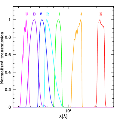
Figure 12.— Filter curves over which rest-frame magnitudes have been computed following Methods 6a_τ, 6a${}_{\tau}^{\rm NEB}$, 6a_delτ and 6a_invτ. Filter curves are available as ascii files in the electronic version of the Journal.

References

- Acquaviva et al. (2011) Acquaviva, V., Gawiser, E., & Guaita, L. 2011, ApJ, 737, 47
- Acquaviva et al. (2012) Acquaviva, V., Gawiser, E., & Guaita, L. 2012, in IAU Symposium, Vol. 284, IAU Symposium, ed. R. J. Tuffs & C. C. Popescu, 42–45
- Anders & Fritze-v. Alvensleben (2003) Anders, P., & Fritze-v. Alvensleben, U. 2003, A&A, 401, 1063
- Ashby et al. (2013) Ashby, M. L. N., Willner, S. P., Fazio, G. G., et al. 2013, ApJ, 769, 80
- Atek et al. (2011) Atek, H., Siana, B., Scarlata, C., et al. 2011, ApJ, 743, 121
- Barro et al. (2011a) Barro, G., Pérez-González, P. G., Gallego, J., et al. 2011a, ApJS, 193, 13
- Barro et al. (2011b) —. 2011b, ApJS, 193, 30
- Barro et al. (2013) Barro, G., Faber, S. M., Pérez-González, P. G., et al. 2013, ApJ, 765, 104
- Behroozi et al. (2013) Behroozi, P. S., Wechsler, R. H., & Conroy, C. 2013, ApJ, 770, 57
- Bertin & Arnouts (1996) Bertin, E., & Arnouts, S. 1996, A&AS, 117, 393
- Bolzonella et al. (2000) Bolzonella, M., Miralles, J.-M., & Pelló, R. 2000, A&A, 363, 476
- Bongiorno et al. (2012) Bongiorno, A., Merloni, A., Brusa, M., et al. 2012, MNRAS, 427, 3103
- Bouwens et al. (2010) Bouwens, R. J., Illingworth, G. D., Oesch, P. A., et al. 2010, ApJ, 709, L133
- Bradshaw et al. (2013) Bradshaw, E. J., Almaini, O., Hartley, W. G., et al. 2013, MNRAS, 433, 194
- Bruzual (2007) Bruzual, G. 2007, in Astronomical Society of the Pacific Conference Series, Vol. 374, From Stars to Galaxies: Building the Pieces to Build Up the Universe, ed. A. Vallenari, R. Tantalo, L. Portinari, & A. Moretti, 303–+
- Bruzual & Charlot (2003) Bruzual, G., & Charlot, S. 2003, MNRAS, 344, 1000
- Calzetti et al. (2000) Calzetti, D., Armus, L., Bohlin, R. C., et al. 2000, ApJ, 533, 682
- Castellano et al. (2014) Castellano, M., Sommariva, V., Fontana, A., et al. 2014, A&A, 566, A19
- Conroy (2013) Conroy, C. 2013, ARA&A, 51, 393
- Conroy & Gunn (2010) Conroy, C., & Gunn, J. E. 2010, ApJ, 712, 833
- Cooper et al. (2012a) Cooper, M. C., Newman, J. A., Davis, M., Finkbeiner, D. P., & Gerke, B. F. 2012a, spec2d: DEEP2 DEIMOS Spectral Pipeline, astrophysics Source Code Library, ascl:1203.003
- Cooper et al. (2011) Cooper, M. C., Aird, J. A., Coil, A. L., et al. 2011, ApJS, 193, 14
- Cooper et al. (2012b) Cooper, M. C., Yan, R., Dickinson, M., et al. 2012b, MNRAS, 425, 2116
- Cooper et al. (2012c) Cooper, M. C., Griffith, R. L., Newman, J. A., et al. 2012c, MNRAS, 419, 3018
- Daddi et al. (2005) Daddi, E., Renzini, A., Pirzkal, N., et al. 2005, ApJ, 626, 680
- Dahlen et al. (2013) Dahlen, T., Mobasher, B., Faber, S. M., et al. 2013, ApJ, 775, 93
- Davis et al. (2003) Davis, M., Faber, S. M., Newman, J., et al. 2003, in Society of Photo-Optical Instrumentation Engineers (SPIE) Conference Series, Vol. 4834, Discoveries and Research Prospects from 6- to 10-Meter-Class Telescopes II, ed. P. Guhathakurta, 161–172
- Davis et al. (2007) Davis, M., Guhathakurta, P., Konidaris, N. P., et al. 2007, ApJ, 660, L1
- Dressler et al. (2011) Dressler, A., Bigelow, B., Hare, T., et al. 2011, PASP, 123, 288
- Duncan et al. (2014) Duncan, K., Conselice, C. J., Mortlock, A., et al. 2014, MNRAS, 444, 2960
- Finkelstein et al. (2012) Finkelstein, S. L., Papovich, C., Salmon, B., et al. 2012, ApJ, 756, 164
- Fioc & Rocca-Volmerange (1997) Fioc, M., & Rocca-Volmerange, B. 1997, A&A, 326, 950
- Fontana et al. (2000) Fontana, A., D’Odorico, S., Poli, F., et al. 2000, AJ, 120, 2206
- Fontana et al. (2006) Fontana, A., Salimbeni, S., Grazian, A., et al. 2006, A&A, 459, 745
- Furusawa et al. (2008) Furusawa, H., Kosugi, G., Akiyama, M., et al. 2008, ApJS, 176, 1
- Galametz et al. (2013) Galametz, A., Grazian, A., Fontana, A., et al. 2013, ApJS, 206, 10
- Geach et al. (2007) Geach, J. E., Simpson, C., Rawlings, S., Read, A. M., & Watson, M. 2007, MNRAS, 381, 1369
- Giallongo et al. (1998) Giallongo, E., D’Odorico, S., Fontana, A., et al. 1998, AJ, 115, 2169
- Giavalisco et al. (2004) Giavalisco, M., Ferguson, H. C., Koekemoer, A. M., et al. 2004, ApJ, 600, L93
- Gladders & Yee (2005) Gladders, M. D., & Yee, H. K. C. 2005, ApJS, 157, 1
- Grazian et al. (2015) Grazian, A., Fontana, A., Santini, P., et al. 2015, accepted by A&A, arXiv: 1412.0532, arXiv:1412.0532
- Grogin et al. (2011) Grogin, N. A., Kocevski, D. D., Faber, S. M., et al. 2011, ApJS, 197, 35
- Guo et al. (2013) Guo, Y., Ferguson, H. C., Giavalisco, M., et al. 2013, ApJS, 207, 24
- Hsu et al. (2014) Hsu, L.-T., Salvato, M., Nandra, K., et al. 2014, ApJ, 796, 60
- Ilbert et al. (2009) Ilbert, O., Capak, P., Salvato, M., et al. 2009, ApJ, 690, 1236
- Ilbert et al. (2010) Ilbert, O., Salvato, M., Le Floc’h, E., et al. 2010, ApJ, 709, 644
- Inoue (2011) Inoue, A. K. 2011, MNRAS, 415, 2920
- Kennicutt (1998) Kennicutt, Jr., R. C. 1998, ARA&A, 36, 189
- Koekemoer et al. (2011) Koekemoer, A. M., Faber, S. M., Ferguson, H. C., et al. 2011, ApJS, 197, 36
- Kriek et al. (2009) Kriek, M., van Dokkum, P. G., Labbé, I., et al. 2009, ApJ, 700, 221
- Laidler et al. (2007) Laidler, V. G., Papovich, C., Grogin, N. A., et al. 2007, PASP, 119, 1325
- Lawrence et al. (2007) Lawrence, A., Warren, S. J., Almaini, O., et al. 2007, MNRAS, 379, 1599
- Lee et al. (2010) Lee, S.-K., Ferguson, H. C., Somerville, R. S., Wiklind, T., & Giavalisco, M. 2010, ApJ, 725, 1644
- Maraston (2005) Maraston, C. 2005, MNRAS, 362, 799
- Maraston et al. (2006) Maraston, C., Daddi, E., Renzini, A., et al. 2006, ApJ, 652, 85
- Maraston et al. (2010) Maraston, C., Pforr, J., Renzini, A., et al. 2010, MNRAS, 407, 830
- Marigo et al. (2008) Marigo, P., Girardi, L., Bressan, A., et al. 2008, A&A, 482, 883
- McLure et al. (2013) McLure, R. J., Pearce, H. J., Dunlop, J. S., et al. 2013, MNRAS, 428, 1088
- Merloni et al. (2010) Merloni, A., Bongiorno, A., Bolzonella, M., et al. 2010, ApJ, 708, 137
- Mobasher et al. (2015) , Dahlen, Ferguson, et al. 2015, subm. to ApJ
- Moustakas et al. (2011) Moustakas, J., Zaritsky, D., Brown, M., et al. 2011, subm. to ApJ, ArXiv: 1112.3300, arXiv:1112.3300
- Moustakas et al. (2013) Moustakas, J., Coil, A. L., Aird, J., et al. 2013, ApJ, 767, 50
- Newman et al. (2013) Newman, J. A., Cooper, M. C., Davis, M., et al. 2013, ApJS, 208, 5
- Papovich et al. (2001) Papovich, C., Dickinson, M., & Ferguson, H. C. 2001, ApJ, 559, 620
- Pérez-González et al. (2008) Pérez-González, P. G., Rieke, G. H., Villar, V., et al. 2008, ApJ, 675, 234
- Pforr et al. (2012) Pforr, J., Maraston, C., & Tonini, C. 2012, MNRAS, 422, 3285
- Pforr et al. (2013) —. 2013, MNRAS, 435, 1389
- Prevot et al. (1984) Prevot, M. L., Lequeux, J., Prevot, L., Maurice, E., & Rocca-Volmerange, B. 1984, A&A, 132, 389
- Rangel et al. (2013) Rangel, C., Nandra, K., Laird, E. S., & Orange, P. 2013, MNRAS, 428, 3089
- Salmon et al. (2015) Salmon, B., Papovich, C., Finkelstein, S. L., et al. 2014, subm. to ApJ, ArXiv: 1407.6012, arXiv:1407.6012
- Santini et al. (2012a) Santini, P., Rosario, D. J., Shao, L., et al. 2012a, A&A, 540, A109
- Santini et al. (2012b) Santini, P., Fontana, A., Grazian, A., et al. 2012b, A&A, 538, A33
- Schaerer & de Barros (2009) Schaerer, D., & de Barros, S. 2009, A&A, 502, 423
- Schaerer & Vacca (1998) Schaerer, D., & Vacca, W. D. 1998, ApJ, 497, 618
- Schenker et al. (2013) Schenker, M. A., Ellis, R. S., Konidaris, N. P., & Stark, D. P. 2013, ApJ, 777, 67
- Simha et al. (2014) Simha, V., Weinberg, D. H., Conroy, C., et al. 2014, ArXiv e-prints, arXiv:1404.0402
- Simpson et al. (2006) Simpson, C., Martínez-Sansigre, A., Rawlings, S., et al. 2006, MNRAS, 372, 741
- Skelton et al. (2014) Skelton, R. E., Whitaker, K. E., Momcheva, I. G., et al. 2014, ArXiv e-prints, arXiv:1403.3689
- Smail et al. (2008) Smail, I., Sharp, R., Swinbank, A. M., et al. 2008, MNRAS, 389, 407
- Stark et al. (2013) Stark, D. P., Schenker, M. A., Ellis, R., et al. 2013, ApJ, 763, 129
- Ueda et al. (2008) Ueda, Y., Watson, M. G., Stewart, I. M., et al. 2008, ApJS, 179, 124
- van Breukelen et al. (2007) van Breukelen, C., Cotter, G., Rawlings, S., et al. 2007, MNRAS, 382, 971
- van der Wel et al. (2006) van der Wel, A., Franx, M., Wuyts, S., et al. 2006, ApJ, 652, 97
- Wiklind et al. (2008) Wiklind, T., Dickinson, M., Ferguson, H. C., et al. 2008, ApJ, 676, 781
- Wiklind et al. (2014) Wiklind, T., Conselice, C. J., Dahlen, T., et al. 2014, ApJ, 785, 111
- Windhorst et al. (2011) Windhorst, R. A., Cohen, S. H., Hathi, N. P., et al. 2011, ApJS, 193, 27
- Wirth et al. (2004) Wirth, G. D., Willmer, C. N. A., Amico, P., et al. 2004, AJ, 127, 3121
- Wuyts et al. (2011) Wuyts, S., Förster Schreiber, N. M., van der Wel, A., et al. 2011, ApJ, 742, 96
- Xue et al. (2011) Xue, Y. Q., Luo, B., Brandt, W. N., et al. 2011, ApJS, 195, 10
- Zibetti et al. (2013) Zibetti, S., Gallazzi, A., Charlot, S., Pierini, D., & Pasquali, A. 2013, MNRAS, 428, 1479