Area and Perimeter of the Convex Hull of Stochastic Points

Abstract

Given a set $P$ of $n$ points in the plane, we study the computation of the probability distribution function of both the area and perimeter of the convex hull of a random subset $S$ of $P$. The random subset $S$ is formed by drawing each point $p$ of $P$ independently with a given rational probability $\pi_{p}$. For both measures of the convex hull, we show that it is #P-hard to compute the probability that the measure is at least a given bound $w$. For $\varepsilon\in(0,1)$, we provide an algorithm that runs in $O(n^{6}/\varepsilon)$ time and returns a value that is between the probability that the area is at least $w$, and the probability that the area is at least $(1-\varepsilon)w$. For the perimeter, we show a similar algorithm running in $O(n^{6}/\varepsilon)$ time. Finally, given $\varepsilon,\delta\in(0,1)$ and for any measure, we show an $O(n\log n+(n/\varepsilon^{2})\log(1/\delta))$-time Monte Carlo algorithm that returns a value that, with probability of success at least $1-\delta$, differs at most $\varepsilon$ from the probability that the measure is at least $w$.

1 Introduction

Let $P$ be a set of $n$ points in the plane, where each point $p$ of $P$ is assigned a probability $\pi_{p}$. Given any subset $X\subset\mathbb{R}^{2}$, let $\mathbb{A}(X)$ and $\mathbb{P}(X)$ denote the area and perimeter, respectively, of the convex hull of $X$. In this paper, we study the random variables $\mathbb{A}(S)$ and $\mathbb{P}(S)$, where $S$ is a random subset of $P$, formed by drawing each point $p$ of $P$ independently with probability $\pi_{p}$. We assume the model in which the probability $\pi_{p}$ of every point $p$ of $P$ is a rational number, and where deciding whether $p$ is present in a random sample of $P$ can be done in constant time. Then, any random sample of $P$ can be generated in $O(n)$ time. We show the following results:

1. Given $w\geq 0$, computing $\Pr[\mathbb{A}(S)\geq w]$ is #P-hard, even in the case where $\pi_{p}=\rho$ for all $p\in P$, for every $\rho\in(0,1)$.

2. Given $w\geq 0$, computing $\Pr[\mathbb{P}(S)\geq w]$ is #P-hard, even in the case where $\pi_{p}\in\{\rho,1\}$ for all $p\in P$, for every $\rho\in(0,1)$.

3. For any measure $\mathsf{m}\in\{\mathbb{A},\mathbb{P}\}$, $w\geq 0$, and $\varepsilon\in(0,1)$, a value $\sigma$ so that $\Pr[\mathsf{m}(S)\geq w]\leq\sigma\leq\Pr[\mathsf{m}(S)\geq(1-\varepsilon)w]$ can be computed in $O(n^{6}/\varepsilon)$ time.

4. For any measure $\mathsf{m}\in\{\mathbb{A},\mathbb{P}\}$ and $\varepsilon,\delta\in(0,1)$, a value $\sigma^{\prime}$ satisfying $\Pr[\mathsf{m}(S)\geq w]-\varepsilon<\sigma^{\prime}<\Pr[\mathsf{m}(S)\geq w]+\varepsilon$ with probability at least $1-\delta$, can be computed in $O(n\log n+(n/\varepsilon^{2})\log(1/\delta))$ time.

5. If $P\subset[0,U]^{2}$ for some $U>0$, then given $\varepsilon\in(0,1)$ and $w\geq 0$, a value $\tilde{\sigma}$ satisfying $\Pr[\mathbb{A}(S)\geq w+\varepsilon]\leq\tilde{\sigma}\leq\Pr[\mathbb{A}(S)\geq w-\varepsilon]$ can be computed in $O(n^{4}\cdot U^{4}/\varepsilon^{2})$ time.

For the ease of explanation, we assume that the point set $P$ satisfies the next properties: no three points of $P$ are collinear, and no two points of $P$ are in the same vertical or horizontal line. All our results can be extended to consider point sets $P$ without these assumptions.

Notation: Given three different points $p,q,r$ in the plane, let $\Delta(p,q,r)$ denote the triangle with vertex set $\{p,q,r\}$, $\ell(p,q)$ denote the directed line through $p$ in direction to $q$, $h(p)$ denote the horizontal line through $p$, $pq$ denote the segment with endpoints $p$ and $q$, and $\overline{pq}$ denote the length of $pq$. We say that a triangle defined by three vertices of the convex hull of a random sample $S\subseteq P$ is canonical if the triangle contains the topmost point of $S$.

Outline: In Section 3, we show that computing the probability that the area is at least a given bound is #P-hard, and provide the algorithms to approximate this probability. In Section 4, we show the results for the perimeter.

2 Related work

Stochastic finite point sets in the plane, as the one considered in this paper, appear in a natural manner in many database scenarios in which the gathered data has many false positives [2, 6, 14]. This model of random points differs from the model in which $n$ points are chosen independently at random in some Euclidean region, and questions related to the final positions of the points are considered [13, 16, 18].

In the last years, algorithmic problems and solutions considering stochastic points have emerged. In 2011, Chan et al. [4] studied the computation of the expectation $\mathbb{E}[MST(S)]$, where $S$ is a random sample drawn on the point set $P$ and $MST(S)$ is the total length of the minimum Euclidean spanning tree of $S$. Each point is included in the sample $S$ independently with a given rational probability. They motivate this problem from the following three situations: the point set $P$ may denote all possible customer locations, each with a known probability of being present at an instant, or it may denote sensors that trigger and upload data at unpredictable times, or it may be a set of multi-dimensional observations, each with a confidence value. Among other results, they proved that computing $\mathbb{E}[MST(S)]$ is #P-hard and provided a random sampling based algorithm running in $O((n^{5}/\varepsilon^{2})\log(n/\delta))$ time, that returns a $(1+\varepsilon)$-approximation with probability at least $1-\delta$. In 2014, Chan et al. [5] studied the probability that the distance of the closest pair of points is at most a given parameter, among $n$ stochastic points. Computing the closest pair of points among a set of precise points is a classic and well-known problem with an efficient solution in $O(n\log n)$ time. When introducing the stochastic imprecision, computing the above probability becomes #P-hard [5].

Foschini at al. [11] studied in 2011 the expected volume of the union of $n$ stochastic axis-aligned hyper-rectangles, where each hyper-rectangle is present with a given probability. They showed that the expected volume can be computed in polynomial time (assuming the dimension is a constant), provided a data structure for maintaining the expected volume over a dynamic family of such probabilistic hyper-rectangles, and proved that it is NP-hard to compute the probability that the volume exceeds a given value even in one dimension, using a reduction from the SubsetSum problem [12].

With respect to the convex hull of stochastic points, in the same model that we consider (called unipoint model [1]), Suri et al. [17] investigated the most likely convex hull of stochastic points, which is the convex hull that appears with the most probability. They proved that such a convex hull can be computed in $O(n^{3})$ time in the plane, and its computation is NP-hard in higher dimensions.

In a more general model of discrete probabilistic points (called multipoint model [1]), each of the $n$ points either does not occur or occurs at one of finitely many locations, following its own discrete probability distribution. In this model that generalizes the one considered in this paper, Agarwal et al. [1] gave exact computations and approximations of the probability that a query point lies in the convex hull, and Feldman et al. [9] considered the minimum enclosing ball problem and gave a $(1+\varepsilon)$-approximation. In this more general model and other ones, Jorgensen et al. [14] studied approximations of the distribution functions of the solutions of geometric shape-fitting problems, and described the variation of the solutions to these problems with respect to the uncertainty of the points. They noted that in the multipoint model the distribution of area or perimeter of the convex hull may have exponential complexity if all the points lie on or near a circle.

More recently, in 2014, Li et al. [15] considered a set of $n$ points in the plane colored with $k$ colors, and studied, among other computation problems, the computation of the expected area or perimeter of the convex hull of a random sample of the points. Such random samples are obtained by picking for each color a point of that color uniformly at random. They proved that both expectations can be computed in $O(n^{2})$ time. We note that their arguments can be used to compute both $\mathbb{E}[\mathbb{A}(S)]$ and $\mathbb{E}[\mathbb{P}(S)]$, each one in $O(n^{2})$ time. In the case of the expected perimeter, similar arguments were discussed by Chan et al. [4].

3 Probability distribution function of area

3.1 #P-hardness

Theorem 1.

Given a stochastic point set $P$ at rational coordinates, an integer $w>0$, and a probability $\rho\in(0,1)$, it is #P-hard to compute the probability $\Pr[\mathbb{A}(S)\geq w]$ that the area of the convex hull of a random sample $S\subseteq P$ is at least $w$, where each point of $P$ is included in $S$ independently with probability $\rho$.

Proof.

We show a Turing reduction from the #SubsetSum problem that is #P-complete [8]. Our Turing reduction assumes an unknown algorithm (i.e. oracle) $\mathcal{A}(P,w)$ computing $\Pr[\mathbb{A}(S)\geq w]$, that will be called twice. The #SubsetSum problem receives as input a set $\{a_{1},\ldots,a_{n}\}\subset\mathbb{N}$ of $n$ numbers and a target $t\in\mathbb{N}$, and counts the number of subsets $J\subseteq[1..n]$ such that $\sum_{i\in J}a_{j}=t$. It remains #P-hard if the subsets $J$ to count must also satisfy $|J|=k$, for given $k\in[1..n]$. Furthermore, we can add a large value (e.g. $1+a_{1}+\dots+a_{n}$) to every $a_{i}$, and add $k$ times this value to the target $t$, so that in the new instance only $k$-element index sets $J$ can add up to the new target. Let $(\{a_{1},\ldots,a_{n}\},t,k)$ be an instance of this restricted #SubsetSum problem. Then, by the above observations, we assume that only sets $J\subseteq[1..n]$ with $|J|=k$ satisfy $\sum_{i\in J}a_{j}=t$. To show that computing $\Pr[\mathbb{A}(S)\geq w]$ is #P-hard, we construct in polynomial time the point set $P$ consisting of the $2n+1$ stochastic points $p_{1},p_{2},\ldots,p_{n+1}$ and $q_{1},q_{2},\ldots,q_{n}$ with the next properties (see Figure 1):

1. $P$ is in convex position and its elements appear as $p_{1},q_{1},p_{2},q_{2},\ldots,p_{n},q_{n},p_{n+1}$ clockwise;

2. the coordinates of $p_{1},\ldots,p_{n+1}$ and $q_{1},\ldots,q_{n}$ are rational numbers, each equal to the fraction of two polynomially-bounded natural numbers;

3. $\pi_{p}=\rho$ for every $p\in P$;

4. for some positive $b\in\mathbb{N}$, $\mathbb{A}(\{p_{j},q_{j},p_{j+1}\})=b\cdot a_{j}\in\mathbb{N}$ for all $j\in[1..n]$;

5. $\mathbb{A}(\{p_{1},\ldots,p_{n+1}\})\in\mathbb{N}$;

6. $\mathbb{A}(\{q_{i},p_{i+1},q_{i+1}\})$ for every $i\in[1..n-1]$, $\mathbb{A}(\{p_{1},q_{1},p_{n+1}\})$, and $\mathbb{A}(\{p_{1},q_{n},p_{n+1}\})$ are all greater than $b\cdot(a_{1}+\dots+a_{n})$.

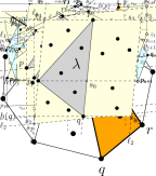
Figure 1: The relative position of the points $p_{1},\ldots,p_{n+1},q_{1},\ldots,q_{n}$.

Let $G=\mathbb{A}(\{p_{1},\ldots,p_{n+1}\})$, and $S\subseteq P$ be any random sample of $P$ such that $\{p_{1},\ldots,p_{n+1}\}\subseteq S$. Let $J_{S}=\{j\in[1..n]\>\lvert\>q_{j}\in S\}$. Observe that

$$\mathbb{A}(S)~{}=~{}G+\sum_{j\in J_{S}}\mathbb{A}(\{p_{j},q_{j},p_{j+1}\})~{}=~{}G+b\sum_{j\in J_{S}}a_{j},$$ (1)

and that for every $J\subseteq[1..n]$ the probability that $J_{S}=J$ is precisely $\rho^{|J|}(1-\rho)^{n-|J|}$. For $x\in\mathbb{N}$, let $f(x)$ denote the number of subsets $J\subseteq[1..n]$ with $x=\sum_{i\in J}a_{i}$, which by the above assumptions satisfy $|J|=k$. Then, the #SubsetSum problem instance asks for $f(t)$. Let $E$ stand for the event in which $\{p_{1},\dots,p_{n+1}\}\subseteq S$, and $\overline{E}$ the complement of $E$. Then,

$$\Pr[\mathbb{A}(S)=G+bt]~{}=~{}\Pr[\mathbb{A}(S)=G+bt\>\lvert\>E]\cdot\Pr[E]+\Pr[\mathbb{A}(S)=G+bt\>\lvert\>\overline{E}]\cdot\Pr[\overline{E}].$$ (2)

When the event $E$ does not occur, that is, when some point $p\in\{p_{1},\dots,p_{n+1}\}$ is not in $S$, we have that the triangle with vertex set $p$ and the two vertices neighboring $p$ in the convex hull of $P$ is missing from the convex hull of $S$. Let

$$\Delta~{}=~{}\min\left\{\begin{array}[]{l}\min_{i\in[1..n-1]}\mathbb{A}(\{q_{i},p_{i+1},q_{i+1}\}),\\ \mathbb{A}(\{p_{1},q_{1},p_{n+1}\}),\\ \mathbb{A}(\{p_{1},q_{n},p_{n+1}\}).\end{array}\right.$$

Then, by property (f), we have that

$$\mathbb{A}(S)~{}\leq~{}\mathbb{A}(P)-\Delta~{}=~{}G+b\cdot(a_{1}+\dots+a_{n})-\Delta~{}<~{}G.$$

Hence, $\mathbb{A}(S)=G+bt$ cannot happen when conditioned in $\overline{E}$. We then continue with equation (2), using equation (1), as follows:

$$\Pr[\mathbb{A}(S)=G+bt] = \Pr[\mathbb{A}(S)=G+bt\>\lvert\>E]\cdot\Pr[E]$$

$$= \Pr\left[\sum_{j\in J_{S}}a_{j}=t,|J_{S}|=k\right]\cdot\Pr[E]$$

$$= \Pr\left[\sum_{j\in J_{S}}a_{j}=t\>\middle\lvert\>|J_{S}|=k\right]\cdot\Pr\bigl{[}|J_{S}|=k\bigr{]}\cdot\Pr[E]$$

$$= \frac{f(t)}{\binom{n}{k}}\cdot\binom{n}{k}\rho^{k}(1-\rho)^{n-k}\cdot\rho^{n+1}$$

$$= f(t)\cdot\rho^{n+k+1}(1-\rho)^{n-k}.$$

Then, we have that

$$f(t)\cdot\rho^{n+k+1}(1-\rho)^{n-k}~{}=~{}\Pr[\mathbb{A}(S)\geq G+bt]-\Pr[\mathbb{A}(S)\geq G+bt+1].$$

Calling twice the algorithm $\mathcal{A}(P,w)$, we can compute $\Pr[\mathbb{A}(S)\geq G+bt]$ and $\Pr[\mathbb{A}(S)\geq G+bt+1]$, and then $f(t)$. Hence, computing $\Pr[\mathbb{A}(S)\geq w]$ is #P-hard.

We show now how the above stochastic point set $P$ can be built in polynomial time. Let $p_{i}=((2i-1)^{2},2i-1)$ for every $i\in[1..n+1]$, and $s_{j}=((2j)^{2},2j)$ for every $j\in[1..n]$. Observe that the points $p_{1},\ldots,p_{n+1},s_{1},\ldots,s_{n}$ belong to $\mathbb{N}^{2}$, are in convex position, and they appear in the order $p_{1},s_{1},p_{2},s_{2},\ldots,p_{n},s_{n},p_{n+1}$ clockwise. Furthermore, $\mathbb{A}(\{p_{i},s_{i},p_{i+1}\})=1$ for all $i\in[1..n]$. Let $\hat{a}=\max\{a_{1},\ldots,a_{n}\}$, and $\lambda_{i}=a_{i}/n\hat{a}$ for $i\in[1..n]$. For every $i\in[1..n]$, we build the point $q_{i}$ on the segment $s_{i}m_{i}$, where $m_{i}=(p_{i}+p_{i+1})/2$ is the midpoint of the segment $p_{i}p_{i+1}$ (see Figure 2).

Figure 2: Construction of the point $q_{i}$ from $p_{i}$, $s_{i}$, and $p_{i+1}$.

The point $q_{i}$ is such that

$$\frac{~{}\overline{q_{i}m_{i}}~{}}{\overline{s_{i}m_{i}}}~{}=~{}\lambda_{i}~{}=~{}\frac{a_{i}}{n\hat{a}}~{}\leq~{}\frac{1}{n}.$$

Observe then that $q_{i}\in\mathbb{Q}^{2}$, and $\mathbb{A}(\{p_{i},q_{i},p_{i+1}\})=\lambda_{i}$ for all $i\in[1..n]$. Finally, we scale the point set $P=\{p_{1},\ldots,p_{n+1},$ $q_{1},\ldots,q_{n}\}$ by $2n\hat{a}$. Let $b=4n\hat{a}$. We have now that

$$\mathbb{A}(\{p_{i},q_{i},p_{i+1}\})~{}=~{}\left(2n\hat{a}\right)^{2}\cdot\lambda_{i}~{}=~{}b\cdot a_{i}~{}\in~{}\mathbb{N},$$

and that $G=\mathbb{A}(\{p_{1},\ldots,p_{n+1}\})\in\mathbb{N}$ since every new $p_{i}$ has even integer coordinates (see Figure 1). By considering $\pi_{p}=\rho$ for every $p\in P$, the point set $P$ ensures the properties (a)-(e). We now show that condition (f) is also ensured. Before scaling by $2n\hat{a}$, we have that

$$m_{i}~{}=~{}(4i^{2}+1,2i)$$

and

$$q_{i}~{}=~{}m_{i}+\lambda_{i}(s_{i}-m_{i})~{}=~{}(4i^{2}+1-\lambda_{i},2i).$$

Then, for $i\in[1..n-1]$,

$$\mathbb{A}(\{q_{i},p_{i+1},q_{i+1}\}) = \frac{1}{2}\left|{\rm~{}det}\begin{bmatrix}4i^{2}+1-\lambda_{i}&2i&1\\ (2i+1)^{2}&2i+1&1\\ 4(i+1)^{2}+1-\lambda_{i+1}&2i+2&1\end{bmatrix}\right|$$

$$= \frac{1}{2}\left|{\rm~{}det}\begin{bmatrix}-\lambda_{i}&0&1\\ 4i&1&1\\ 8i+4-\lambda_{i+1}&2&1\end{bmatrix}\right|$$

$$= \frac{1}{2}\left(4-\lambda_{i}-\lambda_{i+1}\right)$$

$$> 1$$

$$\geq \sum_{j\in[1..n]}\lambda_{j}.$$

After scaling, we will have

$$\mathbb{A}(\{q_{i},p_{i+1},q_{i+1}\})~{}>~{}(2n\hat{a})^{2}\cdot\sum_{j\in[1..n]}\lambda_{j}~{}=~{}b\cdot(a_{1}+\dots+a_{n}).$$

Similarly, assuming $n\geq 2$, before scaling we have

$$\mathbb{A}(\{p_{1},q_{1},p_{n+1}\}) = \frac{1}{2}\left|{\rm~{}det}\begin{bmatrix}1&1&1\\ 5-\lambda_{1}&2&1\\ (2n+1)^{2}&2n+1&1\end{bmatrix}\right|$$

$$= n\lambda_{1}+2n(n-1)$$

$$> 1,$$

and

$$\mathbb{A}(\{p_{1},q_{n},p_{n+1}\}) = \frac{1}{2}\left|{\rm~{}det}\begin{bmatrix}1&1&1\\ 4n^{2}+1-\lambda_{n}&2n&1\\ (2n+1)^{2}&2n+1&1\end{bmatrix}\right|$$

$$= n\lambda_{n}+(2n+1)(n-1)$$

$$> 1.$$

Then, after scaling we will have

$$\mathbb{A}(\{p_{1},q_{1},p_{n+1}\}),\mathbb{A}(\{p_{1},q_{n},p_{n+1}\})>b\cdot(a_{1}+\dots+a_{n}).$$

This shows that property (f) is ensured. The result thus follows. ∎

3.2 Approximations

The idea to approximate $\Pr[\mathbb{A}(S)\geq w]$ is to first consider the fact that when the area of each triangle defined by points of $P$ is a natural number, we can compute such a probability in time polynomial in $n$ and $w$ (see lemmas 2 and 3). After that, the idea follows by using conditionings of the samples $S$ on subsets of $P$ of bounded area of the convex hull, to apply on such conditionings a rounding strategy to the area of each triangle so that each area becomes a natural number, and to use Lemma 2 using the rounded areas instead of the real ones. With the formula of the total probability over the conditionings, we get the approximation to $\Pr[\mathbb{A}(S)\geq w]$.

Lemma 2.

Let $a\in P$, and $E_{a}$ denote the event for the random sample $S\subseteq P$ in which $a$ is the topmost point of $S$. Assuming that the area of each triangle defined by points of $P$ is a natural number, given an integer $w\geq 0$, the probability $\Pr[\mathbb{A}(S)\geq w\mid E_{a}]$ can be computed in $O(n^{3}\cdot w)$ time.

Proof.

We show how to compute the probability $\Pr[\mathbb{A}(S)\geq w\>\lvert\>E_{a}]$ using dynamic programming. Let $B_{a}\subset P$ denote the points below the line $h(a)$, and $\mathbf{P}_{a}\subset(\{a\}\cup B_{a})^{2}$ denote the set of pairs of distinct points $(u,v)$ such that either $v=a$, or $v\neq a$ and $u$ is to the left of the directed line $\ell(a,v)$. For a point $b\in B_{a}$, let $F_{b}$ stand for the event that $b$ is the vertex following $a$ in the counter-clockwise order of the vertices of the convex hull of $(S\cap B_{a})\cup\{a\}$. For every $(u,v)\in\mathbf{P}_{a}$, let $Z_{u,v}\subset\mathbb{R}^{2}$ denote the region of the points below the line $h(a)$, to the left of the line $\ell(a,u)$, and to the left of the line $\ell(v,u)$ (see Figure 3).

Figure 3: The region $Z_{u,v}$. Left: general case. Right: particular case $v=a$.

Now, for every $z\in[0..w]$, consider the entry $T[u,v,z]$ of the table $T$, defined as

$$T[u,v,z]~{}=~{}\Pr\Bigl{[}\mathbb{A}\bigl{(}(S\cap Z_{u,v})\cup\{a,u\}\bigr{)}\geq z\Bigr{]},$$

which stands for the event that the convex hull of the random sample restricted to $Z_{u,v}$, together with the points $a$ and $u$, is at least $z$. Then, note that

$$\Pr\Bigl{[}\mathbb{A}(S)\geq w\>\lvert\>E_{a}\Bigr{]}~{}=~{}\sum_{b\in B_{a}}\Pr\bigl{[}F_{b}\bigr{]}\cdot T[b,a,w].$$ (3)

We show now how to compute $T[u,v,z]$ recursively for every $u,v,z$. For every point $u^{\prime}\in P\cap Z_{u,v}$, let $N_{u^{\prime}}$ stand for the event in which $u^{\prime}$ satisfies the following properties: $u^{\prime}\in S$ and $u^{\prime}$ is the vertex of the convex hull of $(S\cap Z_{u,v})\cup\{a,u\}$ that follows the vertex $u$ in counter-clockwise order, that is, $uu^{\prime}$ is an edge of the convex hull of $(S\cap Z_{u,v})\cup\{a,u\}$ and the elements of $(S\cap Z_{u,v})\setminus\{u^{\prime}\}$ are to the left of the line $\ell(u,u^{\prime})$ (see Figure 4(left)). Note that $u^{\prime}$ is also the first point of $S\cap Z_{u,v}$ hit by the line $\ell(v,u)$ when rotated counter-clockwise centered at $u$. Then, we have that

Figure 4: Computing the entries $T[u,v,z]$ recursively.

$$T[u,v,0]~{}=~{}1~{}~{}\text{ for all }(u,v)\in\mathbf{P}_{a}$$

and

$$T[u,v,z]~{}=~{}\sum_{u^{\prime}\in P\cap Z_{u,v}}\Pr[N_{u^{\prime}}]\cdot F(u,z,u^{\prime})$$

for all $(u,v)\in\mathbf{P}_{a}$ and $z\in[1..w]$, where

$$F(u,z,u^{\prime})~{}=~{}\left\{\begin{array}[]{l}T\bigl{[}u^{\prime},u,z-\mathbb{A}(\{u,u^{\prime},a\})\bigr{]}~{}~{}\text{if}~{}\mathbb{A}(\{u,u^{\prime},a\})<z\\ \\ 1,~{}~{}\text{if}~{}\mathbb{A}(\{u,u^{\prime},a\})\geq z,\end{array}\right.$$

(see Figure 4(right)). Since the points in $P\cap Z_{u,v}$ can be sorted radially around $u$ in $O(n)$ time, by computing the dual arrangement of $P$ in $O(n^{2})$ time as a unique preprocessing, the probabilities $\Pr[N_{u^{\prime}}]$, $u^{\prime}\in P\cap Z_{u,v}$, can be computed in overall $O(n)$ time by following such radial sorting of $P\cap Z_{u,v}$. Then, all entries $T[u,v,z]$ can be computed in $O(n^{3}\cdot w)$ time. Similarly, using the dual arrangement of $P$, the probabilities $\Pr[F_{b}]$, $b\in B_{a}$, can be computed in overall $O(n)$ time, and then $\Pr[\mathbb{A}(S)\geq w\>\lvert\>E_{a}]$ can be computed in linear time using the information of table $T$ and equation (3). Hence, $\Pr[\mathbb{A}(S)\geq w\mid E_{a}]$ can be computed in overall $O(n^{3}\cdot w)$ time. The result thus follows. ∎

Lemma 3.

Assuming that the area of each triangle defined by points of $P$ is a natural number, given an integer $w\geq 0$, the probability $\Pr[\mathbb{A}(S)\geq w]$ can be computed in $O(n^{4}\cdot w)$ time.

Proof.

Observe that we have

$$\Pr\Bigl{[}\mathbb{A}(S)\geq w\Bigr{]}~{}=~{}\sum_{a\in P}\Pr\Bigl{[}\mathbb{A}(S)\geq w\>\lvert\>E_{a}\Bigr{]}\cdot\Pr\Bigl{[}E_{a}\Bigr{]},$$

and that all probabilities $\Pr[E_{a}]$, $a\in P$, can be computed in $O(n)$ time after an $O(n\log n)$-time vertical sorting preprocessing of $P$. Using Lemma 2 to compute $\Pr[\mathbb{A}(S)\geq w\>\lvert\>E_{a}]$ for each $a\in P$, the overall running time to compute $\Pr[\mathbb{A}(S)\geq w]$ is $O(n^{4}\cdot w)$. ∎

Before proving the main result of this section (i.e. Theorem 5), we prove the following useful technical lemma:

Figure 5: Proof of Lemma 4.

Lemma 4.

Let $X$ be a (finite) point set in the plane, $p$ a topmost point of $X$, $q$ a bottommost point of $X$, and $\lambda$ the area of the triangle of maximum area with vertices $p$, $q$, and another point of $X$. Then, we have that:

$$\lambda~{}\leq~{}\mathbb{A}(X)~{}\leq~{}4\lambda.$$

Proof.

Let $r\in X$ be a point such that $\mathbb{A}(\{p,q,r\})=\lambda$, and assume w.l.o.g. that $r$ is to the left of the line $\ell(p,q)$. Let $\ell_{1}$ denote the line through $r$ and parallel to $\ell(p,q)$, and line $\ell_{2}$ the reflection of $\ell_{1}$ about $\ell(p,q)$ (see Figure 5). Let points $s_{0}=\ell(p,q)\cap h(r)$, $s_{1}=\ell_{1}\cap h(q)$, $s_{2}=\ell_{2}\cap h(q)$, $s_{3}=\ell_{2}\cap h(p)$, and $s_{4}=\ell_{1}\cap h(p)$. Note that triangles $\Delta(p,r,s_{0})$ and $\Delta(p,s_{4},r)$ are congruent, and triangles $\Delta(q,s_{0},r)$ and $\Delta(q,r,s_{1})$ are congruent. Furthermore, $X$ is contained in the parallelogram with vertex set $\{s_{1},s_{2},s_{3},s_{4}\}$. Then, we have

$$\mathbb{A}(X) \leq \mathbb{A}(\{s_{1},s_{2},s_{3},s_{4}\})$$

$$= 2\cdot\mathbb{A}(\{s_{1},q,p,s_{4}\})$$

$$= 2\cdot\Bigl{(}\mathbb{A}(\{p,r,s_{0}\})+\mathbb{A}(\{p,s_{4},r\})+\mathbb{A}(\{q,s_{0},r\})+\mathbb{A}(\{q,r,s_{1}\})\Bigr{)}$$

$$= 2\cdot\Bigl{(}2\cdot\mathbb{A}(\{p,r,s_{0}\})+2\cdot\mathbb{A}(\{q,s_{0},r\})\Bigr{)}$$

$$= 4\cdot\mathbb{A}(\{p,q,r\})$$

$$= 4\lambda.$$

Trivially, $\lambda\leq\mathbb{A}(X)$, and the lemma thus follows. ∎

Theorem 5.

Given $\varepsilon\in(0,1)$ and $w\geq 0$, a value $\sigma$ satisfying

$$\Pr[\mathbb{A}(S)\geq w]~{}\leq~{}\sigma~{}\leq~{}\Pr[\mathbb{A}(S)\geq(1-\varepsilon)w]$$

can be computed in $O(n^{6}/\varepsilon)$ time.

Proof.

Given two points $p,q\in P$, let $E_{p,q}$ denote the event in which the random sample $S\subseteq P$ satisfies that: $p$ is the topmost point of $S$, and $q$ is the bottommost point of $S$. Conditioned on the event $E_{p,q}$, for two points $p,q\in P$, let $\lambda=\lambda(p,q)$ denote the area of the triangle of maximum area with vertices $p$, $q$, and another point of $S$. By Lemma 4, we have

$$\lambda~{}\leq~{}\mathbb{A}(S)~{}\leq~{}4\lambda.$$

Furthermore, if $w\leq\lambda$ then $\Pr[\mathbb{A}(S)\geq w\>\lvert\>E_{p,q}]=1$, and if $4\lambda<w$ then $\Pr[\mathbb{A}(S)\geq w\>\lvert\>E_{p,q}]=0$. Then, we can compute $\Pr[\mathbb{A}(S)\geq w]$ as follows:

$$\Pr\bigl{[}\mathbb{A}(S)\geq w\bigl{]} = \sum_{p,q\in P}\Pr\bigl{[}E_{p,q}\bigr{]}\cdot\Pr\bigl{[}\mathbb{A}(S)\geq w\>\lvert\>E_{p,q}\bigr{]}$$ (4)

$$= \sum_{p,q\in P}\Pr\bigl{[}E_{p,q}\bigr{]}\biggl{(}\Pr\bigl{[}\mathbb{A}(S)\geq w\>\lvert\>E_{p,q},\lambda\geq w\bigr{]}\Pr\bigl{[}\lambda\geq w\>\lvert\>E_{p,q}\bigr{]}+$$

$$\Pr\left[\mathbb{A}(S)\geq w\>\lvert\>E_{p,q},\lambda\in\left[\tfrac{w}{4},w\right)\right]\cdot\Pr\left[\lambda\in\left[\tfrac{w}{4},w\right)\>\middle\lvert\>E_{p,q}\right]+$$

$$\Pr\left[\mathbb{A}(S)\geq w\>\lvert\>E_{p,q},\lambda<\tfrac{w}{4}\right]\Pr\left[\lambda<\tfrac{w}{4}\>\middle\lvert\>E_{p,q}\right]\biggr{)}$$

$$= \sum_{p,q\in P}\Pr\bigl{[}E_{p,q}\bigr{]}\biggl{(}\Pr\bigl{[}\lambda\geq w\>\lvert\>E_{p,q}\bigr{]}+$$

$$\Pr\left[\mathbb{A}(S)\geq w\>\middle\lvert\>E_{p,q},\lambda\in\left[\tfrac{w}{4},w\right)\right]\cdot\Pr\left[\lambda\in\left[\tfrac{w}{4},w\right)\>\middle\lvert\>E_{p,q}\right]\biggr{)}.$$

For given $p,q\in P$, and $z\geq 0$, let $P(p,q,z)\subseteq P$ denote the set of the points $r\in P$ lying in the strip bounded by the horizontal lines through $p$ and $q$, respectively, such that $\mathbb{A}(\{p,q,r\})\geq z$. Since

$$\Pr[\lambda\geq z\>\lvert\>E_{p,q}]~{}=~{}1-\prod_{r\in P(p,q,z)}(1-\pi_{r}),$$

both $\Pr[\lambda\geq w\>\lvert\>E_{p,q}]$ and $\Pr[\lambda\in[w/4,w)\>\lvert\>E_{p,q}]=\Pr[\lambda\geq w/4\>\lvert\>E_{p,q}]-\Pr[\lambda\geq w\>\lvert\>E_{p,q}]$ can be computed in $O(n)$ time. To approximate $\Pr[\mathbb{A}(S)\geq w]$ using equation (4), we compute in what follows the value $\sigma_{p,q}\in[0,1]$ as an approximation to the probability $\Pr[\mathbb{A}(S)\geq w\>\lvert\>E_{p,q},\lambda\in[w/4,w)]$. Let $P^{\prime}=P(p,q,0)\setminus P(p,q,w)$, and note that $S\subseteq P^{\prime}$ when conditioned on $E_{p,q}$ and $\lambda\in[w/4,w)$. Let $\theta=\varepsilon/n$. We round the area $a$ of each triangle defined by three points of $P^{\prime}$ by $\widehat{a}=\lceil\frac{a}{\theta\cdot w}\rceil$, and round the target $w$ by $\widehat{w}=\lfloor\frac{1}{\theta}\rfloor$. Let $\widehat{\mathbb{A}}(S)$ be the sum of the rounded areas of the canonical triangles of the convex hull of $S$. Given that the algorithm of Lemma 2 sums areas of canonical triangles, we can run such an algorithm over $P^{\prime}$ by assuming that event $E_{p}$ is satisfied (i.e. $p$ is the topmost point of any random sample $S\subseteq P^{\prime}$) and $\pi_{q}=1$, but considering the rounded areas instead of the original ones. We can make these assumptions because event $E_{p,q}$ holds. Doing this, we can compute the probability $\Pr[\widehat{\mathbb{A}}(S)\geq\widehat{w}\mid E_{p}]$ of Lemma 2, for $S\subseteq P^{\prime}$, in

$$O(n^{3}\cdot\widehat{w})~{}=~{}O\left(n^{3}\cdot\left\lfloor\frac{1}{\theta}\right\rfloor\right)~{}=~{}O(n^{4}/\varepsilon)$$

time, and set $\sigma_{p,q}$ to it. We now analyse how close $\sigma_{p,q}$ is to $\Pr[\mathbb{A}(S)\geq w\>\lvert\>E_{p,q},\lambda\in[w/4,w)]$. Let $S$ be a random sample conditioned on both $E_{p,q}$ and $\lambda\in[w/4,w)$, and so that the convex hull of $S$ is triangulated into $k$ canonical triangles of areas $a_{1},a_{2},\ldots,a_{k}$, respectively. We have

$$w~{}\geq~{}\theta w\left\lfloor\frac{1}{\theta}\right\rfloor~{}=~{}\theta w\cdot\widehat{w}$$

and

$$\theta w\left(\widehat{a_{1}}+\dots+\widehat{a_{k}}\right)~{}=~{}\theta w\left\lceil\frac{a_{1}}{\theta w}\right\rceil+\dots+\theta w\left\lceil\frac{a_{k}}{\theta w}\right\rceil~{}\geq~{}a_{1}+\dots+a_{k}.$$

Then, $a_{1}+\dots+a_{k}\geq w$ implies $\widehat{a_{1}}+\dots+\widehat{a_{k}}\geq\widehat{w}$. Hence,

$$\Pr\Bigl{[}\mathbb{A}(S)\geq w\>\lvert\>E_{p,q},\lambda\in[w/4,w)\Bigr{]}~{}\leq~{}\sigma_{p,q}.$$ (5)

Assume now that $\widehat{a_{1}}+\dots+\widehat{a_{k}}\geq\widehat{w}$. Then, given that

$$\widehat{w}~{}=~{}\left\lfloor\frac{1}{\theta}\right\rfloor~{}\geq~{}\frac{1}{\theta}-1$$

and

$$\widehat{a_{1}}+\dots+\widehat{a_{k}}~{}=~{}\left\lceil\frac{a_{1}}{\theta w}\right\rceil+\dots+\left\lceil\frac{a_{k}}{\theta w}\right\rceil\\ ~{}\leq~{}\frac{a_{1}}{\theta w}+\dots+\frac{a_{k}}{\theta w}+k,$$

we have

$$\frac{a_{1}}{\theta w}+\dots+\frac{a_{k}}{\theta w}+k~{}\geq~{}\frac{1}{\theta}-1$$

which implies

$$a_{1}+\dots+a_{k}~{}\geq~{}w-(k+1)\cdot\theta w~{}\geq~{}w-n\cdot\theta w~{}=~{}(1-n\theta)w~{}=~{}(1-\varepsilon)w.$$

Then, $\widehat{a_{1}}+\dots+\widehat{a_{k}}\geq\widehat{w}$ implies $a_{1}+\dots+a_{k}\geq(1-\varepsilon)w$. Therefore,

$$\sigma_{p,q}~{}\leq~{}\Pr\left[\mathbb{A}(S)\geq(1-\varepsilon)w\>\middle\lvert\>E_{p,q},\lambda\in\left[\tfrac{w}{4},w\right)\right].$$ (6)

We then compute in $O(n^{2}\cdot n^{4}/\varepsilon)=O(n^{6}/\varepsilon)$ time the value

$$\sigma~{}=~{}\sum_{p,q\in P}\Pr\bigl{[}E_{p,q}\bigr{]}\Bigl{(}\Pr\bigl{[}\lambda\geq w\>\lvert\>E_{p,q}\bigr{]}+\sigma_{p,q}\cdot\Pr\left[\lambda\in\left[\tfrac{w}{4},w\right)\>\middle\lvert\>E_{p,q}\right]\Bigr{)},$$

which verifies

$$\Pr\Bigl{[}\mathbb{A}(S)\geq w\Bigr{]}~{}\leq~{}\sigma$$

by equations (4) and (5). Let $w_{\varepsilon}=(1-\varepsilon)w<w$. By equations (4) and (6), $\sigma$ also verifies that

$$\sigma \leq \sum_{p,q\in P}\Pr\bigl{[}E_{p,q}\bigr{]}\biggl{(}\Pr\bigl{[}\lambda\geq w\>\lvert\>E_{p,q}\bigr{]}+$$

$$\Pr\left[\mathbb{A}(S)\geq w_{\varepsilon}\>\lvert\>E_{p,q},\lambda\in\left[\frac{w}{4},w\right)\right]\cdot\Pr\left[\lambda\in\left[\frac{w}{4},w\right)\>\lvert\>E_{p,q}\right]\biggr{)}$$

$$\leq \sum_{p,q\in P}\Pr\bigl{[}E_{p,q}\bigr{]}\biggl{(}\Pr\bigl{[}\lambda\geq w\>\lvert\>E_{p,q}\bigr{]}+$$

$$\Pr\left[\mathbb{A}(S)\geq w_{\varepsilon}\>\middle\lvert\>E_{p,q},\lambda\in\left[\frac{w_{\varepsilon}}{4},w\right)\right]\cdot\Pr\left[\lambda\in\left[\frac{w_{\varepsilon}}{4},w\right)\>\middle\lvert\>E_{p,q}\right]\biggr{)}$$

$$= \sum_{p,q\in P}\Pr\bigl{[}E_{p,q}\bigr{]}\biggl{(}\Pr\bigl{[}\lambda\geq w\>\lvert\>E_{p,q}\bigr{]}+$$

$$\Pr\left[\mathbb{A}(S)\geq w_{\varepsilon}\>\middle\lvert\>E_{p,q},\lambda\in\left[\frac{w_{\varepsilon}}{4},w_{\varepsilon}\right)\right]\cdot\Pr\left[\lambda\in\left[\frac{w_{\varepsilon}}{4},w_{\varepsilon}\right)\>\middle\lvert\>E_{p,q}\right]+$$

$$\Pr\bigl{[}\mathbb{A}(S)\geq w_{\varepsilon}\>\lvert\>E_{p,q},\lambda\in[w_{\varepsilon},w)\bigr{]}\cdot\Pr\bigl{[}\lambda\in[w_{\varepsilon},w)\>\lvert\>E_{p,q}\bigr{]}\biggr{)}$$

$$= \sum_{p,q\in P}\Pr\bigl{[}E_{p,q}\bigr{]}\biggl{(}\Pr\bigl{[}\lambda\geq w\>\lvert\>E_{p,q}\bigr{]}+$$

$$\Pr\left[\mathbb{A}(S)\geq w_{\varepsilon}\>\middle\lvert\>E_{p,q},\lambda\in\left[\frac{w_{\varepsilon}}{4},w_{\varepsilon}\right)\right]\cdot\Pr\left[\lambda\in\left[\frac{w_{\varepsilon}}{4},w_{\varepsilon}\right)\>\middle\lvert\>E_{p,q}\right]+$$

$$\Pr\bigl{[}\lambda\in[w_{\varepsilon},w)\>\lvert\>E_{p,q}\bigr{]}\biggr{)}$$

$$= \sum_{p,q\in P}\Pr\bigl{[}E_{p,q}\bigr{]}\biggl{(}\Pr\bigl{[}\lambda\geq w_{\varepsilon}\>\lvert\>E_{p,q}\bigr{]}+$$

$$\Pr\left[\mathbb{A}(S)\geq w_{\varepsilon}\>\middle\lvert\>E_{p,q},\lambda\in\left[\frac{w_{\varepsilon}}{4},w_{\varepsilon}\right)\right]\cdot\Pr\left[\lambda\in\left[\frac{w_{\varepsilon}}{4},w_{\varepsilon}\right)\>\middle\lvert\>E_{p,q}\right]\biggr{)}$$

$$= \Pr\bigl{[}\mathbb{A}(S)\geq(1-\varepsilon)w\bigr{]}.$$

The result thus follows. ∎

Given the high running time of the algorithm in Theorem 5, and that it may happen that $\Pr[\mathbb{A}(S)\geq(1-\varepsilon)w]-\Pr[\mathbb{A}(S)\geq w]$ is close to 1, we give the following simple Monte Carlo algorithm to approximate $\Pr[\mathbb{A}(S)\geq w]$ with absolute error and a probability of success. A similar algorithm was given by Agarwal et al. [1] to approximate the probability that a given query point is contained in the convex hull of the probabilistic points.

Theorem 6.

Given $\varepsilon,\delta\in(0,1)$ and $w\geq 0$, a value $\sigma^{\prime}$ can be computed in $O(n\log n+(n/\varepsilon^{2})\log(1/\delta))$ time so that with probability at least $1-\delta$

$$\Pr[\mathbb{A}(S)\geq w]-\varepsilon~{}<~{}\sigma^{\prime}~{}<~{}\Pr[\mathbb{A}(S)\geq w]+\varepsilon.$$

Proof.

The idea is to use repeated random sampling. Let $S_{1},S_{2},\ldots,S_{N}\subseteq P$ be $N$ random samples of $P$, where $N$ is going to be specified later, and let $X_{i}$ ($i=1,\ldots,N$) be the indicator variable such that $X_{i}=1$ if and only if $\mathbb{A}(S_{i})\geq w$. Let $\mu=\Pr[\mathbb{A}(S)\geq w]$ and $\sigma^{\prime}=(1/N)\sum_{i=1}^{N}X_{i}$, and note that $\mathbb{E}[X_{i}]=\mu$. Using a Chernoff-Hoeffding bound, we have $\Pr[|\sigma^{\prime}-\mu|\geq\varepsilon]\leq 2\exp(-2\varepsilon^{2}N)$. Then, setting $N=\lceil(1/2\varepsilon^{2})\ln(2/\delta)\rceil$, we have that $|\sigma^{\prime}-\mu|<\varepsilon$ with probability at least $1-\delta$. Since after an $O(n\log n)$-time sorting preprocessing of $P$, the convex hull of each sample $S_{i}$ can be computed in $O(n)$ time, the running time is $O(n\log n+N\cdot n)=O(n\log n+(n/\varepsilon^{2})\log(1/\delta))$. ∎

If the coordinates of the points of $P$ belong to some range of bounded size, then we can round the coordinates of each point of $P$ so that in the resulting point set every triangle defined by three points has integer area. After that, we can use Lemma 3 over the resulting point set to approximate the probability $\Pr[\mathbb{A}(S)\geq w]$. This approach is used in the following result.

Theorem 7.

If $P\subset[0,U]^{2}$ for some $U>0$, then given $\varepsilon\in(0,1)$ and $w\geq 0$ a value $\tilde{\sigma}$ satisfying

$$\Pr[\mathbb{A}(S)\geq w+\varepsilon]~{}\leq~{}\tilde{\sigma}~{}\leq~{}\Pr[\mathbb{A}(S)\geq w-\varepsilon]$$

can be computed in $O(n^{4}\cdot U^{4}/\varepsilon^{2})$ time.

Proof.

Let $\delta>0$ be a parameter to be specified later. For every random sample $S\subseteq P$, let

$$\tilde{S}~{}=~{}\left\{\left(2\left\lfloor\frac{x}{\delta}\right\rfloor,2\left\lfloor\frac{y}{\delta}\right\rfloor\right)~{}:~{}(x,y)\in S\right\}.$$

Note that the area of every triangle defined by three points of $\tilde{S}$ is a natural number, for every $S\subseteq P$. Furthermore, we have that

$$\left|\mathbb{A}(S)-\left(\frac{\delta^{2}}{4}\right)\mathbb{A}(\tilde{S})\right|~{}<~{}4\delta U.$$

Using Lemma 3, we can compute the probability

$$\tilde{\sigma}~{}=~{}\Pr\left[\mathbb{A}(\tilde{S})\geq\left\lceil\frac{4w}{\delta^{2}}\right\rceil\right]$$

in $O\left(n^{4}\cdot\left\lceil 4w/\delta^{2}\right\rceil\right)\subseteq O\left(n^{4}\cdot U^{2}/\delta^{2}\right)$ time. If $\mathbb{A}(\tilde{S})\geq\left\lceil 4w/\delta^{2}\right\rceil$, then

$$w~{}\leq~{}\mathbb{A}(\tilde{S})\cdot\frac{\delta^{2}}{4}~{}<~{}\mathbb{A}(S)+4\delta U,$$

which implies $\mathbb{A}(S)~{}\geq~{}w-4\delta U$. Hence,

$$\tilde{\sigma}~{}=~{}\Pr\left[\mathbb{A}(\tilde{S})\geq\left\lceil 4w/\delta^{2}\right\rceil\right]~{}\leq~{}\Pr\Bigl{[}\mathbb{A}(S)\geq w-4\delta U\Bigr{]}.$$ (7)

If $\mathbb{A}(S)\geq w+4\delta U$, then

$$w+4\delta U~{}\leq~{}\mathbb{A}(S)~{}<~{}\frac{\delta^{2}}{4}\cdot\mathbb{A}(\tilde{S})+4\delta U,$$

which implies $\mathbb{A}(\tilde{S})\geq\left\lceil 4w/\delta\right\rceil$ since $\mathbb{A}(\tilde{S})\in\mathbb{N}$. Then, we have that

$$\Pr\Bigl{[}\mathbb{A}(S)\geq w+4\delta U\Bigr{]}~{}\leq~{}\Pr\left[\mathbb{A}(\tilde{S})\geq\left\lceil 4w/\delta^{2}\right\rceil\right]~{}=~{}\tilde{\sigma}.$$ (8)

Setting $\delta=\frac{\varepsilon}{4U}$, and combining (7) and (8), we have that $\tilde{\sigma}$ satisfies

$$\Pr[\mathbb{A}(S)\geq w+\varepsilon]~{}\leq~{}\tilde{\sigma}~{}\leq~{}\Pr[\mathbb{A}(S)\geq w-\varepsilon],$$

and can be computed in $O(n^{4}U^{4}/\varepsilon^{2})$ time. ∎

4 Perimeter

Similar to Lemma 3, we can prove that if all the distances between the elements of $P$ are considered integer, the probability $\Pr[\mathbb{P}(S)\geq w]$ can be computed in $O(n^{4}\cdot w)$ time, for every integer $w\geq 0$. Then, using conditioning of the samples and a rounding strategy, we adapt the arguments of Theorem 5 to obtain the following result:

Theorem 8.

Given $\varepsilon\in(0,1)$ and $w\geq 0$, a value $\sigma^{\prime}$ satisfying

$$\Pr[\mathbb{P}(S)\geq w]~{}\leq~{}\sigma^{\prime}~{}\leq~{}\Pr[\mathbb{P}(S)\geq(1-\varepsilon)w]$$

can be computed in $O(n^{6}/\varepsilon)$ time.

We can further show that Theorem 6 also holds if perimeter is used instead of area, as stated in the next more general theorem.

Theorem 9.

Let $\mathsf{m}:2^{P}\rightarrow\mathbb{R}$ be a function such that after a $T(n)$-time preprocessing of $P$ the value of $\mathsf{m}(S)$ can be computed in $C(n)$ time, for all $S\subseteq P$. Given $\varepsilon,\delta\in(0,1)$ and $w\geq 0$, a value $\sigma^{\prime}$ can be computed in $O(T(n)+C(n)\cdot(1/\varepsilon^{2})\log(1/\delta))$ time so that with probability at least $1-\delta$

$$\Pr[\mathsf{m}(S)\geq w]-\varepsilon~{}<~{}\sigma^{\prime}~{}<~{}\Pr[\mathsf{m}(S)\geq w]+\varepsilon.$$

Note that for $\mathsf{m}\in\{\mathbb{A},\mathbb{P}\}$ we will have $T(n)=O(n\log n)$ and $C(n)=O(n)$. We complement this section by proving that, in general, computing the probability $\Pr[\mathbb{P}(S)\geq w]$ is #P-hard. The arguments are similar to that of Theorem 1, but the proof requires several key details to deal with distances between points, expressed by square roots. We note that this hardness result (see next Theorem 10) is weaker than that of Theorem 1 in the sense that it uses points with two different probabilities.

Theorem 10.

Given a stochastic point set $P$ at rational coordinates, an integer $w>0$, and a probability $\rho\in(0,1)$, it is #P-hard to compute the probability $\Pr[\mathbb{P}(S)\geq w]$ that the perimeter of the convex hull of a random sample $S\subseteq P$ is at least $w$, where each point of $P$ is included in $S$ independently with a probability in $\{\rho,1\}$.

Proof.

We show a Turing reduction from the version of the #SubsetSum problem [8], in which given numbers $\{a_{1},\ldots,a_{n}\}\subset\mathbb{N}$, a target $t$, and value $k\in[1..n]$, counts the number of subsets $J$ such that $|J|=k$ and $\sum_{j\in J}a_{j}=t$. Let $(\{a_{1},\ldots,a_{n}\},t,k)$ be an instance of this #SubsetSum problem. We assume that $\{a_{1},\ldots,a_{n}\}$ and $t$ are such that only subsets $J$ satisfying $|J|=k$ ensure that $\sum_{j\in J}a_{j}=t$ (see the proof of Theorem 1). Furthermore, each of the numbers $a_{1},\ldots,a_{n}$ can be represented in a polynomial number of bits (refer to the NP-completeness proof of the SubsetSum problem [12]), then the base-2 logarithm of each of them is polynomially bounded. Let $c\in\mathbb{N}$ be a big enough and polynomially bounded number that will be specified later. For every $k\in[1..2n]$, let $v_{k}$ denote de vector

$$v_{k}~{}=~{}\left(c\cdot\frac{k^{2}-1}{k^{2}+1},c\cdot\frac{2k}{k^{2}+1}\right).$$

Let $p_{1}=(0,0)$, and for $i=1,\dots,n$, let $s_{i}=p_{i}+v_{2i-1}$ and $p_{i+1}=s_{i}+v_{2i}$. Let $z_{1}=p_{n+1}-v_{1}$, and for $j=2,\ldots,2n-1$, let $z_{j}=z_{j-1}-v_{j}$. Note that the $4n$ points $p_{1},s_{1},p_{2},s_{2},\ldots,p_{n},s_{n},p_{n+1},$ $z_{1},\ldots z_{2n-1}$ are at rational coordinates and in convex position, and appear in this order clockwise. Further note that each edge of the convex hull of those points has length precisely $c$, and that the perimeter is equal to $L=4n\cdot c\in\mathbb{N}$ (see Figure 6).

Figure 6: The points $p_{1},s_{1},p_{2},s_{2},\ldots,p_{n},s_{n},p_{n+1}$, $z_{1},\ldots z_{2n-1}$ built using the vectors $v_{1},v_{2},\ldots,v_{2n}$.

Let $\varepsilon=1/(2n)$. For every $i\in[1..n]$, we build in polynomial time the point $q_{i}\in\mathbb{Q}^{2}$ in the triangle $\Delta(p_{i},s_{i},p_{i+1})$ so that

$$c-a_{i}~{}\leq~{}\overline{p_{i}q_{i}}~{}=~{}\overline{q_{i}p_{i+1}}~{}<~{}(c-a_{i})+\varepsilon.$$

The value of $c$ is selected so that the point $q_{i}$ exists for every $i\in[1..n]$. Let $P$ denote the point set $\{p_{1},s_{1},p_{2},s_{2},\ldots,p_{n},s_{n},p_{n+1},z_{1},\ldots z_{2n-1}\}\cup\{q_{1},\ldots,q_{n}\}$, and let $\pi_{u}=1$ for all $u\in\{p_{1},p_{2},\ldots,p_{n},p_{n+1},z_{1},\ldots z_{2n-1}\}\cup\{q_{1},\ldots,q_{n}\}$, and $\pi_{v}=\rho$ for all $v\in\{s_{1},\ldots,s_{n}\}$. Let $S\subseteq P$ be any random sample of $P$, $J_{S}=\{j\in[1..n]\>\lvert\>s_{j}\notin S\}$, and $\varepsilon_{j}=\overline{p_{j}q_{j}}-(c-a_{j})$ for every $j\in[1..n]$. Observe that

$$\mathbb{P}(S) = 2n\cdot c~{}+~{}\sum_{j\in J_{S}}2\cdot\overline{p_{j}q_{j}}~{}+~{}\sum_{j\notin J_{S}}2c$$

$$= 2n\cdot c~{}+~{}\sum_{j\in J_{S}}2\left((c-a_{i})+\varepsilon_{j}\right)~{}+~{}\sum_{j\notin J_{S}}2c$$

$$= L~{}-~{}2\sum_{j\in J_{S}}a_{j}~{}+~{}2\sum_{j\in J_{S}}\varepsilon_{j},$$

which implies that

$$L~{}-~{}2\sum_{j\in J_{S}}a_{j}~{}=~{}\left\lfloor\mathbb{P}(S)\right\rfloor,$$

given that

$$0~{}\leq~{}2\sum_{j\in J_{S}}\varepsilon_{j}~{}<~{}2|J_{S}|\cdot\varepsilon~{}\leq~{}2n\cdot\varepsilon~{}=~{}1.$$

For $x\in\mathbb{N}$, let $f(x)$ denote the number of subsets $J\subseteq[1..n]$ with $x=\sum_{i\in J}a_{i}$, which satisfy $|J|=k$. For every $J\subseteq[1..n]$, the probability that $J_{S}=J$ is precisely $(1-\rho)^{|J|}\rho^{n-|J|}$. Then,

$$\Pr\bigl{[}\left\lfloor\mathbb{P}(S)\right\rfloor=L-2t\bigr{]}~{}=~{}\Pr\left[\sum_{j\in J_{S}}a_{j}=t,|J_{S}|=k\right]~{}=~{}f(t)\cdot(1-\rho)^{k}\rho^{n-k}.$$

Hence, computing $\Pr[\mathbb{P}(S)\geq w]$ is #P-hard since

$$\Pr\bigl{[}\left\lfloor\mathbb{P}(S)\right\rfloor~{}=~{}L-2t\bigr{]}~{}=~{}\Pr\bigl{[}\mathbb{P}(S)\geq L-2t\bigr{]}-\Pr\bigl{[}\mathbb{P}(S)\geq L-2t+1\bigr{]}.$$

We show now how to compute the value of $c$, and how to compute the point $q_{i}$ for every $i\in[1..n]$. Consider the isosceles triangle $\Delta(p_{i},s_{i},p_{i+1})$ (see Figure 7).

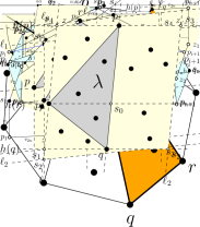
Figure 7: Construction of the point $q_{i}$.

Let $m_{i}$ denote the midpoint of the segment $p_{i}p_{i+1}$, and $s=2i-1$. To ensure the existence of a point $\tilde{q_{i}}\in s_{i}m_{i}$ such that $\overline{p_{i}\tilde{q_{i}}}=c-a_{i}$, we need to guarantee that

$$(c-a_{i})^{2} > \overline{p_{i}m_{i}}^{2}$$

$$= \frac{c^{2}}{4}\left(\left(\frac{s^{2}-1}{s^{2}+1}+\frac{(s+1)^{2}-1}{(s+1)^{2}+1}\right)^{2}+\left(\frac{2s}{s^{2}+1}+\frac{2(s+1)}{(s+1)^{2}+1}\right)^{2}\right)$$

$$= \frac{c^{2}}{2}\left(1+\frac{s^{2}-1}{s^{2}+1}\cdot\frac{(s+1)^{2}-1}{(s+1)^{2}+1}+\frac{2s}{s^{2}+1}\cdot\frac{2(s+1)}{(s+1)^{2}+1}\right)$$

$$= \frac{c^{2}}{2}\left(1+\frac{s^{4}+2s^{3}+3s^{2}+2s}{s^{4}+2s^{3}+3s^{2}+2s+2}\right)$$

$$= c^{2}\left(1-\frac{1}{s^{4}+2s^{3}+3s^{2}+2s+2}\right),$$

which holds if

$$\left(1-\frac{a_{i}}{c}\right)^{2}~{}\geq~{}\left(1-\frac{1}{20s^{4}}\right)^{2}~{}~{}~{}(\text{i.e. }c~{}\geq~{}20s^{4}a_{i})$$

since

$$\left(1-\frac{1}{20s^{4}}\right)^{2}~{}>~{}1-\frac{1}{10s^{4}}~{}\geq~{}1-\frac{1}{s^{4}+2s^{3}+3s^{2}+2s+2}.$$

Then, we set $c=20\cdot(2n)^{4}\cdot\max\{a_{1},\ldots,a_{n}\}=320\cdot n^{4}\cdot\max\{a_{1},\ldots,a_{n}\}$.

Let $d=\overline{p_{i}m_{i}}$ and $z=\overline{\tilde{q_{i}}m_{i}}^{2}=(c-a_{i})^{2}-d^{2}\in\mathbb{Q}$. The point $q_{i}$ is a point in the segment $s_{i}m_{i}$, that is close to $\tilde{q_{i}}$, such that, if $h$ denotes the distance $\overline{q_{i}m_{i}}$, then $h$ is rational and satisfies

$$\sqrt{z}~{}\leq~{}h~{}<~{}\sqrt{z}+\delta,$$

where $\delta=\frac{1}{2^{k+1}}$ and $k=\lfloor\log_{2}((1+2\sqrt{z})/\varepsilon^{2})\rfloor$. Note that $k$ can be computed in $O(\log(z/\varepsilon))\subseteq O(\log(c/\varepsilon))\subseteq O(\log n+\log c)\subseteq O(\log c)$ time, which polynomial in the size of the input. Further note that $h$ can be found, by using a binary search, in polynomial $O(\log(\sqrt{z}/\delta))\subseteq O(\log c)$ time. Then, we have

$$h^{2}-z~{}=~{}(h-\sqrt{z})(h+\sqrt{z})~{}<~{}\delta(\delta+2\sqrt{z})~{}<~{}\delta(1+2\sqrt{z})~{}<~{}\varepsilon^{2},$$

which implies

$$(c-a_{i})^{2}~{}\leq~{}d^{2}+h^{2}~{}<~{}(c-a_{i})^{2}+\varepsilon^{2}~{}<~{}\left((c-a_{i})+\varepsilon\right)^{2}.$$

Hence,

$$c-a_{i}~{}\leq~{}\sqrt{d^{2}+h^{2}}~{}=~{}\overline{p_{i}q_{i}}~{}=~{}\overline{q_{i}p_{i+1}}~{}<~{}(c-a_{i})+\varepsilon.$$

Since the slope of the line $\ell(p_{i},p_{i+1})$ is rational, the slope of $\ell(s_{i},m_{i})$ is also rational. Then, $q_{i}$ has rational coordinates since $\overline{q_{i}m_{i}}=h\in\mathbb{Q}$. ∎

5 Discussion

The results of this paper consider the unipoint model: each point has a fixed location but exists with a given probability. The arguments given for approximating the probability distribution functions of area and perimeter, respectively, seem not to work in the multipoint model, in which each point exists probabilistically at one of multiple possible sites. For the unipoint model, both the expectation and the probability distribution function of the number of vertices in the convex hull can be computed exactly in polynomial time. It suffices to consider either that the area of each triangle defined by three points is equal to one, or that the segment defined by each pair of points has length equal to one, and then use Lemma 3 of this paper. With respect to our dynamic-programming approaches, similar dynamic-programming algorithms have been given by Eppstein et al. [7], Fischer [10], and Bautista et al. [3].

References

- [1] P. K. Agarwal, S. Har-Peled, S. Suri, H. Yıldız, and W. Zhang. Convex hulls under uncertainty. In ESA’14, pages 37–48. 2014.
- [2] P. Agrawal, O. Benjelloun, A. Das Sarma, C. Hayworth, S. U. Nabar, T. Sugihara, and J. Widom. Trio: A system for data, uncertainty, and lineage. In VLDB’06, pages 1151–1154, 2006.
- [3] C. Bautista-Santiago, J. M. Díaz-Báñez, D. Lara, P. Pérez-Lantero, J. Urrutia, and I. Ventura. Computing optimal islands. Operations Research Letters, 39(4):246–251, 2011.
- [4] T. M. Chan, P. Kamousi, and S. Suri. Stochastic minimum spanning trees in Euclidean spaces. In SOCG’11, pages 65–74, 2011.
- [5] T. M. Chan, P. Kamousi, and S. Suri. Closest pair and the post office problem for stochastic points. Computational Geometry, 47(2, Part B):214–223, 2014.
- [6] G. Cormode, F. Li, and K. Yi. Semantics of ranking queries for probabilistic data and expected ranks. In ICDE’09, pages 305–316, 2009.
- [7] D. Eppstein, M. Overmars, G. Rote, and G. Woeginger. Finding minimum area -gons. Discrete & Computational Geometry, 7(1):45–58, 1992.
- [8] P. Faliszewski and L. Hemaspaandra. The complexity of power-index comparison. Theoretical Computer Science, 410(1):101–107, 2009.
- [9] D. Feldman, A. Munteanu, and C. Sohler. Smallest enclosing ball for probabilistic data. In SOCG’14, pages 214–223, 2014.
- [10] P. Fischer. Sequential and parallel algorithms for finding a maximum convex polygon. Computational Geometry, 7(3):187–200, 1997.
- [11] L. Foschini, J. Hershberger, S. Suri, and H. Yıldız. The union of probabilistic boxes: Maintaining the volume. In ESA’11, pages 591–602. 2011.
- [12] M. R. Garey and D. S. Johnson. Computers and Intractability: A Guide to the Theory of NP-Completeness. W. H. Freeman & Co., NY, USA, 1979.
- [13] S. Har-Peled. On the expected complexity of random convex hulls, 2011. arXiv preprint arXiv:1111.5340.
- [14] A. Jorgensen, M. Löffler, and J. M. Phillips. Geometric computations on indecisive and uncertain points, 2012. arXiv preprint arXiv:1205.0273.
- [15] C. Li, C. Fan, J. Luo, F. Zhong, and B. Zhu. Expected computations on color spanning sets. Journal of Combinatorial Optimization, 29(3):589–604, 2015.
- [16] R. Schneider. Discrete aspects of stochastic geometry. In J. E. Goodman and J. O’Rourke, editors, Handbook of Discrete and Computational Geometry, pages 255–278. CRC Press, 2004.
- [17] S. Suri, K. Verbeek, and H. Yıldız. On the most likely convex hull of uncertain points. In ESA’13, pages 791–802. 2013.
- [18] J. G. Wendel. A problem in geometric probability. Mathematica Scandinavica, 11:109–111, 1962.