Separated Response Functions in
Exclusive, Forward $\bf{\pi}^{\pm}$ Electroproduction on Deuterium

Abstract

Background

Measurements of forward exclusive meson production at different squared four-momenta of the exchanged virtual photon, $Q^{2}$, and at different four-momentum transfer, $t$, can be used to probe QCD’s transition from meson-nucleon degrees of freedom at long distances to quark-gluon degrees of freedom at short scales. Ratios of separated response functions in $\pi^{-}$ and $\pi^{+}$ electroproduction are particularly informative. The ratio for transverse photons may allow this transition to be more easily observed, while the ratio for longitudinal photons provides a crucial verification of the assumed pole dominance, needed for reliable extraction of the pion form factor from electroproduction data.

Purpose

Perform the first complete separation of the four unpolarized electromagnetic structure functions $L$/$T$/$LT$/$TT$ in forward, exclusive $\pi^{\pm}$ electroproduction on deuterium above the dominant resonances.

Method

Data were acquired with 2.6-5.2 GeV electron beams and the HMS+SOS spectrometers in Jefferson Lab Hall C, at central $Q^{2}$ values of 0.6, 1.0, 1.6 GeV² at $W$=1.95 GeV, and $Q^{2}=2.45$ GeV² at $W$=2.22 GeV. There was significant coverage in $\phi$ and $\epsilon$, which allowed separation of $\sigma_{L,T,LT,TT}$.

Results

$\sigma_{L}$ shows a clear signature of the pion pole, with a sharp rise at small $-t$. In contrast, $\sigma_{T}$ is much flatter versus $t$. The longitudinal/transverse ratios evolve with $Q^{2}$ and $t$, and at the highest $Q^{2}=2.45$ GeV² show a slight enhancement for $\pi^{-}$ production compared to $\pi^{+}$. The $\pi^{-}/\pi^{+}$ ratio for transverse photons exhibits only a small $Q^{2}$-dependence, following a nearly universal curve with $t$, with a steep transition to a value of about 0.25, consistent with $s$-channel quark knockout. The $\sigma_{TT}$/$\sigma_{T}$ ratio also drops rapidly with $Q^{2}$, qualitatively consistent with $s$-channel helicity conservation. The $\pi^{-}/\pi^{+}$ ratio for longitudinal photons indicates a small isoscalar contamination at $W$=1.95 GeV, consistent with what was observed in our earlier determination of the pion form factor at these kinematics.

Conclusions

The separated cross sections are compared to a variety of theoretical models, which generally describe $\sigma_{L}$ but have varying success with $\sigma_{T}$. Further theoretical input is required to provide a more profound insight into the relevant reaction mechanisms for longitudinal and transverse photons, such as whether the observed transverse ratio is indeed due to a transition from pion to quark knockout mechanisms, and provide useful information regarding the twist-3 transversity generalized parton distribution, $H_{T}$.

I Introduction

Exclusive electroproduction is a powerful tool for the study of nucleon structure. In contrast to inclusive $(e,e^{\prime})$ or photoproduction measurements, the transverse momentum of a scattering constituent (and thus its transverse size is proportional to $1/\sqrt{-t}$) can be probed in addition to its longitudinal momentum, and independent of the momentum transfer $Q^{2}$ to this constituent. Exclusive forward pion electroproduction is especially interesting because the longitudinal and transverse virtual photon polarizations act as a filter on the spin and hence the type of the participating constituents. By detecting the charge of the pion, even the flavor of the constituents can be tagged. Finally, ratios of separated response functions can be formed for which nonperturbative corrections may cancel, yielding insight into soft-hard factorization at the modest $Q^{2}$ to which exclusive measurements will be limited for the foreseeable future. The full potential of pion electroproduction is only now being realized due to the availability of high-luminosity, multi-GeV beams at the Thomas Jefferson National Accelerator Facility (Jefferson Lab, or JLab).

Four amplitudes contribute to pion electroproduction from a nucleon in the Born approximation, where a single virtual photon $\gamma^{*}$ emitted by the electron couples to the hadronic system: pion-pole, nucleon-pole, crossed nucleon-pole and contact term. The first three amplitudes correspond to Mandelstam $t$, $s$ and $u$-channel processes, respectively, Fig. 1. The contact term is used to restore gauge invariance. Born-amplitude based models  Ber70 ; Gut72 indicate that for values of the invariant mass $W$ above the resonance region and for not too large values of $Q^{2}$, the longitudinal part $\sigma_{L}$ of the cross section for pion electroproduction at small values of $-t$ is dominated by the $t$-channel process. The other response functions (transverse $\sigma_{T}$ and interference terms $\sigma_{LT}$ and $\sigma_{TT}$) are relatively small. In this regime, the process can be viewed as quasi-elastic scattering of the electron from a virtual pion and thus is sensitive to the pion form factor, $F_{\pi}$. At values of $t$ approaching the pion mass squared (the so called $t$-pole), the longitudinal response function becomes approximately proportional to the square of the charged pion form factor

$$\sigma_{L}\approx\frac{-tQ^{2}}{(t-M^{2}_{\pi})^{2}}g^{2}_{\pi NN}(t)F^{2}_{\pi}(Q^{2},t).$$ (1)

Here, the factor $g_{\pi NN}(t)$ comes from the $\pi NN$ vertex and represents the probability amplitude to have a virtual charged $\pi$ meson inside the nucleon at a given $t$.

Figure 1: Born diagrams for $\pi^{+}$ electroproduction from a proton.

In order to reliably extract $F_{\pi}$, the $t$-pole process should be dominant in the kinematic region under study. This dominance can be studied experimentally through the ratio of longitudinal $\gamma^{*}_{L}n\to\pi^{-}p$ and $\gamma^{*}_{L}p\to\pi^{+}n$ cross sections, which can be expressed in terms of contributions from isoscalar $A_{S}$ and isovector $A_{V}$ photon amplitudes:

$$R_{L}\equiv\frac{\gamma_{L}^{*}n\to\pi^{-}p}{\gamma_{L}^{*}p\to\pi^{+}n}=\frac{|A_{V}-A_{S}|^{2}}{|A_{V}+A_{S}|^{2}}.$$ (2)

The $t$-channel process proceeds purely via isovector amplitudes. Interference terms between the isoscalar and isovector photon amplitudes have opposite signs for $\pi^{+}$ and $\pi^{-}$ production, which leads to a difference in the cross sections if significant isoscalar contributions are present. Hence, where the $t$-pole dominates (small $-t$), the ratio $R_{L}$ is expected to be close to unity. A departure from $R_{L}=1$ would indicate the presence of isoscalar backgrounds arising from mechanisms such as $\rho$ meson exchange VGL1 or perturbative contributions due to transverse quark momentum Milana . Such physics backgrounds may be expected to be larger at higher $-t$ (due to the drop-off of the pion pole contribution) or non-forward kinematics (due to angular momentum conservation) raskin . Because previous data are unseparated Brauel1 , no firm conclusions about possible deviations of $R_{L}$ from unity were possible.

One can also use such hard exclusive processes to investigate the range of applicability of QCD factorization and scaling theorems. The most important of these is the handbag factorization, where only one parton participates in the hard subprocess, and the soft physics is encoded in generalized parton distributions (GPDs). The handbag approach applies to deep exclusive meson production, where $Q^{2}$ is large and $-t$ is small collins ; eides . For longitudinal photons with $Q^{2}>10$ GeV² and $-t\ll M_{N}^{2}$, this theorem allows one to relate exclusive $N(e,e^{\prime}\pi^{\pm})N$ observables to integrals over the quark flavor-dependent GPDs. Pseudoscalar meson-production observables not dominated by the pion pole term, such as $\sigma_{T}$ in exclusive $\pi^{\pm}$ electroproduction, have also been identified as being especially sensitive to the chiral-odd transverse GPDs ahmad ; gk10 . However, large higher-order corrections Belitsky have delayed the application of GPDs to pion electroproduction until recently. The model of Refs. gk10 ; gk13 uses a modified perturbative approach based on GPDs, incorporating the empirical pion electromagnetic form factor and significant contributions from the twist-3 transversity GPD, $H_{T}$, which gives substantial strength in the transverse cross section.

In the transition region between low $-t$ (where a description of hadronic degrees of freedom in terms of effective hadronic Lagrangians is valid) and large $-t$ (where the degrees of freedom are quarks and gluons), $t$-channel exchange of a few Regge trajectories permits an efficient description of the energy-dependence and the forward angular distribution of many real- and virtual-photon-induced reactions. The VGL Regge model VGL ; VGL1 has provided a good and consistent description of a wide variety of $\pi^{\pm}$ photo- and electroproduction data above the resonance region, as well as of the $p(e,e^{\prime}\pi^{+})n$ reaction using longitudinally polarized virtual photons. However, the model has consistently failed to provide a good description of $p(e,e^{\prime}\pi^{+})n$ $\sigma_{T}$ data Blok08 . The VGL Regge model was recently extended kaskulov ; vrancx by the addition of a hard deep-inelastic scattering (DIS) of virtual photons off nucleons. The DIS process dominates the transverse response at moderate and high $Q^{2}$, providing a better description of $\sigma_{T}$. By assuming that the exclusive $\sigma_{T}$ cross section behaves as $\sigma_{T}^{\text{DIS}}(Q^{2})\propto F_{1}^{p}(x,Q^{2})$, the authors predict that at moderate $Q^{2}$

$$R_{T}\equiv\frac{\sigma_{T}^{\pi^{-}}}{\sigma_{T}^{\pi^{+}}}\approxeq\frac{F_{1}^{n}}{F_{1}^{p}}\approx\frac{F_{2}^{n}}{F_{2}^{p}}<1.$$ (3)

Our purpose was to perform a complete $L$/$T$/$LT$/$TT$ separation in exclusive forward $\pi^{\pm}$ electroproduction on the proton and neutron. Because there are no practical free neutron targets, the ²H$(e,e^{\prime}\pi^{\pm})NN_{s}$ reactions (where $N_{s}$ denotes the spectator nucleon) were used. As those reactions proceed via quasi-free production, the results can be used to compare $\pi^{-}$ production on the neutron to $\pi^{+}$ production on the proton, particularly if ratios are formed. However, due to binding effects, the $\pi^{+}$ results on the deuteron may differ from those on the proton, which were taken in the same kinematics. The data were obtained in Hall C at JLab as part of the two pion form factor experiments presented in detail in Ref. Blok08 . The purpose of this paper is to describe the experiment and analysis of these data in detail, concentrating on those parts that differ from our ¹H$(e,e^{\prime}\pi^{+})n$ study Ref. Blok08 .

This paper is organized as follows. Sec II describes the experiment and the determination of the various efficiencies that are applied in calculating the cross sections. Sec III presents the determination of the unseparated cross sections, their separation into the $L$/$T$/$LT$/$TT$ structure functions, and the systematic uncertainties. Sec IV discusses these results and compares them with various theoretical calculations. The paper is concluded with a short summary.

II Experiment and Data Analysis

The analysis procedures applied here were also used in our recent letter on ²H$(e,e^{\prime}\pi^{\pm})NN_{s}$ results Huber14 . For details of the experiment and the analysis not discussed here, we refer the reader to the discussion of our ¹H experiment Blok08 .

II.1 Experiment and Kinematics

The two $F_{\pi}$ experiments were carried out in 1997 (F_π-1) and 2003 (F_π-2) in Hall C at JLab. For the measurements presented here, the unpolarized electron beam from the CEBAF accelerator was incident on a liquid deuterium target. Two moderate acceptance, magnetic focusing spectrometers were used to detect the particles of interest. The spectrometer settings correspond to either ²H$(e,e^{\prime}\pi^{+})nn_{s}$ or ²H$(e,e^{\prime}\pi^{-})pp_{s}$ kinematics, where the Short Orbit Spectrometer (SOS) was always used to detect the scattered electron, and the High Momentum Spectrometer (HMS) was used to detect the high momentum $\pi^{+}$ or $\pi^{-}$.

The choice of kinematics for the two experiments was based on maximizing the range in $Q^{2}$ for a value of the invariant mass $W$ above the resonance region, while still enabling a longitudinal-transverse separation. The value $W$=1.95 GeV used in the first experiment is high enough to suppress most $s$-channel baryon resonance backgrounds, but this suppression should be even more effective at the $W$=2.2 GeV of the second experiment. For each $Q^{2}$, data were taken at two values of the virtual photon polarization, $\epsilon$, with $\Delta\epsilon>$0.25. This allowed for a separation of the longitudinal and transverse cross sections. Constraints on the kinematics were imposed by the maximum available electron energy, the maximum central momentum of the SOS, and the minimum HMS angle. In parallel kinematics, i.e., when the pion spectrometer is situated in the direction of the $\vec{q}$ vector, the acceptances of the two spectrometers do not provide a uniform coverage in $\phi_{\pi}$. Thus, to attain full coverage in $\phi_{\pi}$ and allow a separation of the interference $LT$ and $TT$ cross sections, additional data were taken in most cases with the HMS at a slightly smaller and larger angle compared to the central angle for the high $\epsilon$ settings. At low $\epsilon$, only the larger angle setting was possible. The kinematic settings are summarized in Table 1.

	2H$(e,e^{\prime}\pi^{+})nn$	2H$(e,e^{\prime}\pi^{-})pp$
Fπ-1 Settings
$Q^{2}$=0.6 GeV2, $W=$1.95 GeV
$\epsilon$=0.37, $E_{e}=$2.445 GeV	3 HMS settings: $\Theta_{\pi q}$=+0.5, +2.0, +4.0o	2 HMS settings: +0.5, +4.0o
$\epsilon$=0.74, $E_{e}=$3.548 GeV	4 HMS settings: $\Theta_{\pi q}$=-2.7, 0.0, +2.0, +4.0o	1 HMS setting: 0.0o
$Q^{2}$=0.75 GeV2, $W=$1.95 GeV
$\epsilon$=0.43, $E_{e}=$2.673 GeV	2 HMS settings: $\Theta_{\pi q}$=0.0, +4.0o	2 HMS settings: $\theta_{\pi q}$=0.0, +4.0o
$\epsilon$=0.70, $E_{e}=$3.548 GeV	3 HMS settings: $\Theta_{\pi q}$=-4.0, 0.0, +4.0o	No data
$Q^{2}$=1.0 GeV2, $W=$1.95 GeV
$\epsilon$=0.33, $E_{e}=$2.673 GeV	2 HMS settings: $\Theta_{\pi q}$=0.0, +4.0o	2 HMS settings: $\theta_{\pi q}$=0.0, +4.0o
$\epsilon$=0.65, $E_{e}=$3.548 GeV	3 HMS settings: $\Theta_{\pi q}$=-4.0, 0.0, +4.0o	1 HMS setting: 0.0o
$Q^{2}$=1.6 GeV2, $W=$1.95 GeV
$\epsilon$=0.27, $E_{e}=$3.005 GeV	2 HMS settings: $\Theta_{\pi q}$=0.0, +4.0o	Same settings as $\pi^{+}$
$\epsilon$=0.63, $E_{e}=$4.045 GeV	3 HMS settings: $\Theta_{\pi q}$=-4.0, 0.0, +4.0o	Same settings as $\pi^{+}$
Fπ-2 Settings
$Q^{2}$=2.45 GeV2, $W=$2.2 GeV
$\epsilon$=0.27, $E_{e}=$4.210 GeV	2 HMS settings: $\Theta_{\pi q}$=+1.35, +3.0o	Same settings as $\pi^{+}$
$\epsilon$=0.55, $E_{e}=$5.248 GeV	3 HMS settings: $\Theta_{\pi q}$=-3.0, 0.0, +3.0o	Same settings as $\pi^{+}$

Table 1: A summary of the ²H kinematic settings taken in the two pion form factor experiments. The angle $\Theta_{\pi q}$ refers to the lab angle between the pion spectrometer and the central $\vec{q}$-vector as defined by the beam energy and the angle of the electron spectrometer.

For each $Q^{2}$, $\epsilon$ setting, the electron spectrometer angle and momentum, as well as the pion spectrometer momentum, were kept fixed. The HMS magnetic polarity was reversed between $\pi^{+}$ and $\pi^{-}$ running, with the quadrupoles and dipole magnets cycled according to a standard procedure, then set to the final values by current (in the case of the quadrupoles) or by NMR probe (in the case of the dipole).

Kinematic offsets in spectrometer angle and momentum, as well as in beam energy, were previously determined using elastic $ep$ coincidence data taken during the same run, and the reproducibility of the optics was checked Blok08 . For the deuterium data sets studied here, elastic runs on ¹H were used to check the validity of the HMS and SOS corrections for several momentum ranges. The reproducibility of the optics was checked during electron running with sieve slits and by the position of the missing mass peak for ²H$(e,e^{\prime}\pi^{+})nn_{s}$ or ²H$(e,e^{\prime}\pi^{-})pp_{s}$. No shifts beyond the expected calibration residuals $\pm$2 MeV were observed Volmerthesis ; Tanjathesis .

II.2 HMS Tracking and Tracking Efficiency

The HMS singles rates were much higher for the $\pi^{-}$ settings than the $\pi^{+}$ settings because of the large electron background at negative spectrometer polarity, so accurate HMS track reconstruction at high rates is needed. Charged particle trajectories are measured by two drift chambers, each with six planes chambers . All data presented here used the track selection criterion that 5 out of 6 planes in each drift chamber for both spectrometers should have a valid signal. This criterion is much better suited to high rate data (in this case the $\pi^{-}$ channel data) than the analysis of our earlier F_π-1 $\pi^{+}$ data from hydrogen target volmer ; tadevosyan , which used a 4/6 tracking selection criterion for HMS and 5/6 for SOS tracking.

The HMS tracking algorithm used here is the same as used in our earlier F_π-2 analysis from liquid hydrogen target hornt . The algorithm has several requirements:

• If the program reconstructed only one track, then that track was used.

• If two or more tracks are reconstructed, then the track that projects to the blocks in the calorimeter measuring the energy deposit (i.e. the cluster) was used. The calorimeter cut used was quite loose to only eliminate “noise” tracks in the chambers.

• In case two or more tracks hit the cluster in the calorimeter (or neither of them), then additional criteria based on which hodoscope bar was hit were used to select a correct track.

The above criteria ensured that the chosen track was the most likely one to have resulted from the trigger for that event and greatly reduced the number of events improperly excluded from the analysis.

The fiducial tracking inefficiencies were 2-9% for HMS rates up to 1.4 MHz. The tracking efficiency is defined as the ratio of the number of events for which an actual track is found, to the ‘events’ that pass through the drift chambers. This ratio is extracted from events in a fiducial area where it is extremely likely that the scintillator hits are due to particles that also traversed the chambers. The tracking efficiency depends on both the drift chamber hit efficiency and the tracking algorithm used in finding the track.

In order to accurately calculate the tracking efficiency, tight particle identification (PID) requirements were applied to select a pure data sample. These requirements are stricter than those used in the regular analysis. In the HMS, the particle identification requirements used to select pions in the tracking efficiency calculation consisted of cuts on the gas C̆erenkov and the calorimeter for F_π-1 data, while for F_π-2 an additional cut on the aerogel C̆erenkov was applied.

The fiducial tracking efficiency analysis also incorporates a cut on the integrated pulse (ADC) from the scintillator hodoscope PMTs, to exclude events with multiple hits per scintillator plane. In the case where there are multiple tracks in the same scintillator plane, this cut places a bias on the event sample used to calculate the tracking efficiency. Since 2-track events have a lower efficiency than 1-track events, the resulting bias causes the HMS tracking efficiency to be overestimated.

To obtain a better understanding of the HMS tracking efficiencies, in F_π-2 a study of singles yields from a carbon target versus HMS rate and beam current was performed. The normalized yields from a carbon target should present no significant beam current- or rate-dependence if the various efficiencies are calculated correctly. Unfortunately, no luminosity scans on carbon target were taken at different beam currents in the F_π-1 experiment, so any conclusions obtained from the F_π-2 study have to be applied also to the F_π-1 data.

Since the probability of a second particle traversing the HMS during the event resolving time is greater at high rates, a tight electron PID cut might introduce its own deadtime not due to tracking efficiency, causing the rate-dependence to be underestimated. Therefore, only HMS fiducial acceptance cuts were applied in this study. Normalized yields from the carbon target were computed from the number of events passing cuts, the integrated beam charge, the electronic and CPU data acquisition livetimes and the HMS tracking efficiency. They are plotted versus rate in Fig. 2. The error bars include statistical uncertainties and an estimated systematic uncertainty of 0.3% added in quadrature, to take into account beam steering on the target and other sensitive effects when no PID cut is applied. Data from the two kinematic settings were separately fit versus rate (dashed red and dash-dot blue curves in the figure) and normalized to unity at zero rate. The two data sets, thus normalized, were then fit together, yielding the solid black curve. The observed rate-dependence suggests that the fiducial HMS tracking efficiencies $htr$, as determined using the procedure described at the start of this section, should be corrected in the following manner

$$htr^{\prime}=htr(e^{-6.76236\cdot 10^{-5}\times\text{HMSrate(kHz)}}).$$ (4)

This is particularly important for the F_π-1 $\pi^{-}$ runs, which are at higher HMS rate.

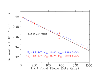
Figure 2: (Color online) Normalized yields (no PID cut) from the carbon target versus HMS singles rate. As the tracking efficiency calculation uses a data sample where multiple track events are rejected, the HMS tracking efficiencies are overestimated at high rates, leading to an effective drop in normalized yield versus rate. The HMS tracking efficiencies for both of the F_π-1 and F_π-2 data sets are corrected with the linear rate dependent function shown here, leading to a normalized yield that is independent of rate.

The systematic uncertainties in the HMS tracking efficiencies were estimated as follows. In the F_π-2 hydrogen analysis, the tracking efficiencies were assigned a 1.0% scale and an 0.4% $\epsilon$-uncorrelated systematic uncertainty, where the first is the scale uncertainty common to all settings, and the second is due to a variety of factors that may affect high and low $\epsilon$ settings differently, as evidenced by the greater scatter exhibited by the tracking efficiencies at high rates (see Refs. Tanjathesis ; Blok08 and Sec. III.5). There is an additional uncertainty of 0.2%/MHz due to the tracking efficiency correction shown in Fig. 2. Since the maximum rate variation for all F_π-2 $\pi^{\pm}$ settings, as well as the F_π-1 $\pi^{+}$ settings, is about 400 kHz, this gives a total $\epsilon$-uncorrelated systematic uncertainty of 0.45%. The F_π-1 $\pi^{-}$ $\epsilon$-uncorrelated systematic uncertainty is somewhat larger. Since the high rate scatter in these $\pi^{-}$ tracking efficiencies is approximately $\pm 1.25\%$ at 1.3 MHz, we assign an $\epsilon$-uncorrelated systematic uncertainty for these settings of 1.3%.

In addition to the above tracking efficiencies, the experimental yields were also corrected for data acquisition electronic and CPU dead time. The correction ranged from 1-11% with minimal uncertainty, as discussed in Refs. Blok08 ; Volmerthesis .

II.3 Cryotarget Boiling Correction

When the electron beam hits a liquid target, it deposits a large power per unit target area and as a result induces localized density fluctuations referred to as “target boiling.” In order to reduce these fluctuations, the beam was rastered over a small area rather than localizing it at one point on the target. The target boiling effect can be measured by comparing the yields at fixed kinematics and varying beam current. During both experiments (F_π-1 and F_π-2), dedicated luminosity elastic runs were taken for both liquid targets (hydrogen and deuterium). The two experiments used cryotargets with significantly different geometries, as well as significantly different beam raster patterns, leading to very different boiling effects.

F_π-2 used the “tuna can” cryotarget geometry and circular beam raster design, which are expected to result in boiling corrections $<1\%$ Tanjathesis . To determine the appropriate correction when the corrected HMS tracking efficiencies are used, data were acquired in dedicated runs with a wide variety of electron beam currents for all $\pi^{-}$ kinematic settings except $Q^{2}$=2.45 GeV², high $\epsilon$, $E_{e}=5.25$ GeV, $\theta_{\text{HMS}}=13.61^{\circ}$. Only fiducial acceptance cuts were applied in this study, and normalized singles yields from these ²H negative polarity HMS data were computed from the number of counts passing cuts, the integrated beam charge, electronic and CPU data acquisition livetimes, and the HMS tracking efficiencies corrected via Eqn. 4. The observed current-dependence suggests that no correction should be applied, which is similar to the conclusion reached in Ref. Tanjathesis for a liquid ¹H target of the same shape and dimensions.

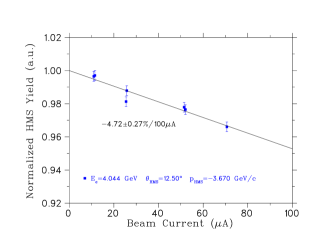
Figure 3: (Color online) Normalized HMS yields from F_π-1 ²H elastics data taken with an electron trigger plotted as a function of beam current. A +0.2$~{}\mu$A beam current offset is applied, as described in the text. The error bars include statistical uncertainties and an estimated systematic uncertainty of 0.3% added in quadrature.

F_π-1 used the so-called “soda can” cryotarget geometry and “bed post” beam rastering, which leads to a significant boiling correction. The magnitude of this correction is sensitive to the rate-dependent correction applied to the HMS tracking efficiencies. The HMS tracking efficiencies were corrected via Eqn. 4 and normalized yields calculated in the same manner as in the F_π-2 cryotarget boiling study. In analyzing these data, it was found that the slope of yield versus beam current was overly sensitive to the inclusion of the lowest current points in the fit. The beam current calibration has an inherent 0.2 $\mu$A uncertainty due to noise in the Unser monitor. A sigificantly reduced sensitivity to these low current points was obtained with the addition of a +0.2 $\mu$A beam current offset, which was subsequently applied in all F_π-1 yield calculations was determined via a $\chi^{2}$ minimization technique. A similar current offset was used in Ref.  Gaskellthesis .

The corrected data were thus fit versus current and normalized to unity at zero current, yielding the black curve in Fig. 3, and a ²H target density correction of $(4.72\pm 0.27\%)/100~{}\mu$A. This correction is particularly important for the F_π-1 $\pi^{+}$ data. Since the HMS detector rates were lower when the HMS was set at positive polarity compared to negative polarity, higher incident electron beam currents were often used for the $\pi^{+}$ runs. The resulting cryotarget boiling correction is similar to the $(6\pm 1\%)/100~{}\mu$A correction determined for the F_π-1 ¹H cell in Ref. Volmerthesis .

II.4 HMS C̆erenkov Blocking Correction

The potential contamination by electrons when the pion spectrometer is set to negative polarity, and by protons when it is set to positive polarity, introduces some differences in the $\pi^{\pm}$ data analyses which were carefully examined. For most negative HMS polarity runs, electrons were rejected at the trigger level by a gas C̆erenkov detector containing C₄F₁₀ at atmospheric pressure acting as a veto in order to avoid high DAQ deadtime due to large $e^{-}$ rates in the HMS. There is a loss of pions due to electrons passing through the HMS gas C̆erenkov within $\sim$100 ns after a pion has traversed the detector, resulting in a mis-identification of the pion event as an electron and being eliminated by the PID cuts applied (C̆erenkov blocking). To reduce this effect, the beam current was significantly reduced during $\pi^{-}$ running. Two independent studies were performed to determine the correction that should be applied to both experiments.

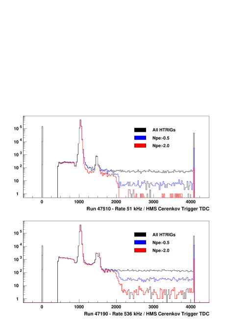
Figure 4: (Color online) HMS C̆erenkov Trigger multi-hit TDC histograms for two F_π-2 runs with C̆erenkov veto disabled. The top panel is a low rate run, and the bottom panel is a high rate run. HMS singles events, subject to a variety of indicated C̆erenkov cuts, are used in both spectra. The TDC scale is 100 ps/chan. Please see the text for further information.

In our first study, the timing spectra features of the C̆erenkov signal into the HMS trigger were investigated for a variety of F_π-2 $\pi^{-}$ runs with HMS singles rates between 7 kHz and $\sim$600 kHz. The multi-hit TDC is started by the HMS pretrigger signal and can be stopped multiple times by the retimed (i.e. delayed and discriminated) C̆erenkov signal (Fig. 4). The main peak corresponds to signals (primarily electrons) that result in the trigger, starting the TDC. Events not associated with the original trigger (other electrons or pions) appear as additional events to the left and right of the main electron peak. The second peak to the right is due to a second electron arriving within the timing window, but after the discriminator “dead window” of $\sim$40 ns (caused by the length of the discriminator pulse). The backgrounds to the left and right of the two peaks are due to earlier and later electrons, while the tail extending to channel 4096 is due to pedestal noise that crosses the discriminator threshold. The peak at channel 4096 is the accumulation of very late TDC stops, while zeros correspond to electrons (or pions) that did not give a stop.

As indicated by the differences between the low rate and high rate runs plotted in Fig. 4, the main peak to pedestal ratio degrades with increasing rate, and the second peak to first peak ratio gets larger. The width of the portion of the TDC spectrum corresponding to electrons traversing the detector current-to or after the original trigger particle indicated that the effective C̆erenkov TDC gate width was 116.4$\pm$ 6.3 ns for the F_π-2 $\pi^{-}$ runs, where the uncertainty is estimated from the slopes and widths of the TDC spectra features. We confirmed that the basic features of the TDC spectra are the same for HMS singles and HMS+SOS coincidences. We also compared the TDC spectra for five pairs of $\pi^{-}$ runs, where for each pair the beam and rate conditions were identical but in one run the HMS C̆erenkov veto was disabled and in the other it was enabled. The spectra for runs with C̆erenkov trigger veto had a much greater proportion of events where no TDC stop was recorded, due to the C̆erenkov signal being below the discriminator threshold. From the normalized differences of these pairs of runs we estimated that the C̆erenkov trigger was about 90% efficient at vetoing electrons.

A comparison of $\pi^{-}$ runs with same rate but different trigger condition can also be used to determine the effective threshold of the C̆erenkov trigger veto. The normalized difference of C̆erenkov photoelectron (ADC) spectra was formed for each pair of runs, and the excess of counts at a large number of photoelectrons when the veto was disabled indicated an effective veto threshold of approximately 2.5 photoelectrons. Because PMT gain variations and pile-up effects will cause the actual veto threshold to vary with rate, a slightly more restrictive software threshold on the number of photoelectrons detected in the HMS C̆erenkov, $hcer_{\text{npe}}<2.0$, was uniformly applied in the F_π-2 data analysis to cut out electrons.

In our second study, we made use of the same dedicated F_π-2 $\pi^{-}$ runs already used to determine the liquid deuterium cryotarget boiling correction. The C̆erenkov veto was disabled in all of these runs, and the beam current was varied over a wide range for each $\pi^{-}$ kinematic setting except for the high $\epsilon$ setting at $Q^{2}$=2.45 GeV², $E_{e}=5.25$ GeV, $\theta_{\text{HMS}}=13.61^{\circ}$. HMS fiducial and $hcer_{\text{npe}}<2.0$ cuts were applied to these HMS singles data, and the normalized $\pi^{-}$ yields (with HMS tracking efficiency corrected by Eqn. 4) were plotted versus HMS electron rate. The normalized pion yield is expected to drop with rate because of electrons passing through the C̆erenkov detector within the trigger gate width after a pion has traversed the detector. The rate-dependences of the normalized pion yields at each kinematic setting were consistent within their (large) uncertainties, and yielded an average gate width of $\tau=139\pm 19$ ns. Note that this study depends upon the tracking efficiency and cryotarget boiling corrections used, while the first study based on the C̆erenkov TDC spectra does not. Finally, since the $\tau$ value from the second study was determined with singles events, it needs to be adjusted to yield the effective gate width for coincidence events. This correction is determined from the portion of the C̆erenkov TDC spectrum corresponding to early electrons passing through the detector before the particle associated with the trigger, yielding $99.2\pm 19$ ns.

The two F_π-2 C̆erenkov blocking studies (TDC gate width of $116.4\pm 6.3$ ns and corrected singles value of $99.2\pm 19$ ns) are consistent within uncertainties. It is difficult to tell which one is more definitive, so the error weighted average $\tau_{\text{eff}}=114.7\pm 6.0$ ns, is used to compute the C̆erenkov blocking correction $\delta_{\text{CCblock}}=e^{-(\text{ELECTRONrate})\cdot\tau_{\text{{eff}}}}$ for the F_π-2 $\pi^{-}$ analysis. For the F_π-2 $\pi^{-}$ data, the HMS electron rate varied from nearly zero to $\sim$600 kHz, resulting in a C̆erenkov blocking correction of 0-6%. The $\pm 6.0$ ns uncertainty gives an uncorrelated systematic uncertainty of 0.3% at 500 kHz, while the 17 ns difference in $\tau$ values from the two methods gives a scale uncertainty of 0.8%.

$\pi^{-}$ data without C̆erenkov veto at different rates were unfortunately not taken during the F_π-1 experiment, so the C̆erenkov blocking correction cannot be directly determined for those data. We therefore modify the C̆erenkov blocking correction determined from F_π-2 data for use in the F_π-1 analysis according to the following procedure. A HMS C̆erenkov photoelectron histogram for a carbon elastics run taken at the very beginning of F_π-1, immediately before the first $\pi$ data run, indicates that the effective veto threshold in the F_π-1 experiment is slightly lower than that used in F_π-2. Therefore, a slightly more restrictive software threshold of $hcer_{\text{npe}}<1.5$ was applied in the analysis of the F_π-1 data. The figure also indicates that the C̆erenkov veto would be about 80% efficient for this run.

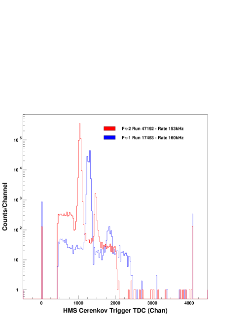
Figure 5: (Color online) HMS C̆erenkov Trigger TDC histogram for the one F_π-1 $\pi^{-}$ run with C̆erenkov veto disabled (blue), compared to a F_π-2 run with same trigger at similar rate (red). HMS singles events, subject to a $hcer_{\text{npe}}>2.0$ C̆erenkov cut, are used in both spectra. The TDC scale is 100 ps/chan.

We therefore reanalyzed the F_π-2 dedicated $\pi^{-}$ runs without C̆erenkov veto, except that a $hcer_{\text{npe}}<1.5$ C̆erenkov particle identification appropriate to the F_π-1 analysis was applied. The dependence of normalized pion singles yields on rate yielded a value of $\tau=162\pm 19$ ns, which was then adjusted to give an effective gate width for coincidence events of $116\pm 20$ ns. Finally, we used the TDC timing information from the only F_π-1 “open trigger” run taken just before the main data taking to estimate the scaling with respect to the F_π-2 timing information. As shown in Fig. 5, the TDC timing window used during F_π-1 is wider than in F_π-2. Comparing the equivalent features of the two spectra gives a scale factor of $1.19\pm 0.084$. Application of this scale factor to the $\tau$ value determined from the F_π-2 data yields $\tau=(115.7\pm 20)\times(1.19\pm 0.084)=137.7\pm 26$ ns.

The two values compare well (TDC gate width of $138.4\pm 6.3$ ns and corrected singles value of $137.7\pm 26$ ns) and thus the error-weighted average $\tau_{\text{eff}}=138.4\pm 6.1$ ns of the two was taken as the effective $\tau$ value to compute the C̆erenkov blocking corrections for the F_π-1 data normalization. For the F_π-1 $\pi^{-}$ data, the HMS electron rate varied from nearly zero to $\sim$1.2 MHz, resulting in a C̆erenkov blocking correction of 0-15%. The $\pm 6.1$ ns uncertainty gives an uncorrelated systematic uncertainty of 0.7% at 1.2 MHz, and scaling the 0.8% F_π-2 scale uncertainty to 1.2 MHz gives a scale uncertainty of 1.0%.

II.5 Other Particle Identification Corrections

Fig. 6 shows the HMS particle speed, $\beta=v/c$, which is calculated from the time-of-flight difference between two scintillator planes in the HMS detector stack. The upper band events are $\pi^{+}$ in the HMS, with the 2 ns beam structure of the incident electron beam clearly visible. The lower band events are protons. In both F_π-1 and F_π-2, a cut $\beta>0.95$ was used to eliminate the protons. Additionally in the F_π-2 experiment, an aerogel C̆erenkov detector was used for separating protons and $\pi^{+}$ for HMS central momenta above 3 GeV/c.

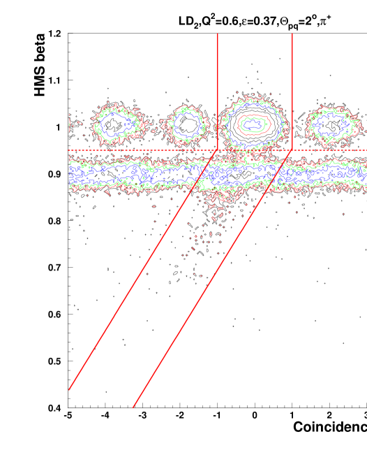
Figure 6: (Color online) HMS+SOS coincindence time versus $\beta_{\text{HMS}}$ for a representative F_π-1 $\pi^{+}$ run. The dashed line indicates the $\beta>0.95$ cut used to separate pions from protons. The solid lines indicate the region (for $\pi^{-}$ runs, without proton contamination) used to compute the $\beta$ cut correction. See the text for more details.

Figure 6 also displays a “tail” at low ${\beta_{\text{HMS}}}$ due to pions undergoing nuclear interactions in the scintillators, C̆erenkov detector material, and in the case of F_π-2 experiment, the aerogel C̆erenkov detector material. A correction for pion events at lower $\beta$ eliminated by the $\beta>0.95$ cut was applied. In F_π-1 this correction was extracted from the $\pi^{-}$ data and was applied to both the $\pi^{-}$ and $\pi^{+}$ data sets. The correction was 4.89%, with an uncertainty of 0.41% determined from the standard deviation of the correction determined from the different $\pi^{-}$ kinematic settings. For the F_π-2 data, the same procedure was used, except that the aerogel C̆erenkov detector permitted the separation of protons from pions, leading to a cleaner pion sample. For each $\pi^{+}$ and $\pi^{-}$ kinematic setting, “beta cut corrections” were extracted in the same fashion, yielding average $\beta$ cut corrections of $2.42\%\pm 0.12\%$ and $2.51\%\pm 0.18\%$ for $\pi^{+}$ and $\pi^{-}$, respectively.

A correction for the number of pions lost due to pion nuclear interactions and true absorption in the HMS exit window and detector stack of 1-2% was also applied. For details on how this correction was determined, see Ref. Blok08 .

A comprehensive summary of the various corrections applied to the data is given in Table 2.

Summary of Fπ-1 Correction Factors
HMS tracking efficiency correction	$1-(0.0676\pm 0.002)/$S1Xrate(MHz)	Sec. II.2
LD2 Cryotarget Boiling	$1-(0.0472\pm 0.003)/100~{}\mu$A	Sec. II.3
Beam Current Offset	$0.2\mu$A	Sec. II.3
HMS C̆erenkov blocking	$e^{{\rm-(\text{ELECTRONrate})}\cdot(138.4\pm 6.1~{}{\rm ns})}$	Sec. II.4
$\beta_{cut}$ correction ($\pi^{\pm}$)	$4.89\%\pm 0.41\%$	Sec. II.5
Pion Absorption	$1\%\pm 1\%$	Sec. II.5, Ref. Blok08
SOS C̆erenkov efficiency	$99.92\%\pm 0.02\%$	Ref. Tanjathesis
SOS Calorimeter efficiency	$99.5\%\pm 0.1\%$	Ref. Tanjathesis
HMS C̆erenkov efficiency	$99.6\%\pm 0.05\%$	Ref. Tanjathesis
Coincidence Time Blocking	$e^{{\rm-TotalPretrigrate}\cdot(140~{}{\rm ns})}$	Ref. Volmerthesis
HMS electronic live time	$1-5/6(N_{h60}-N_{h120})/N_{\text{hELREAL}}$	Ref. Volmerthesis
SOS electronic live time	$1-5/6(N_{s60}-N_{s120})/N_{\text{sELREAL}}$	Ref. Volmerthesis
Summary of Fπ-2 Correction Factors
HMS tracking efficiency correction	$1-(0.0676\pm 0.002)/$S1Xrate(MHz)	Sec. II.2
LD2 Cryotarget Boiling	No correction. $\pm 0.3\%/100~{}\mu A$	Sec. II.3
HMS C̆erenkov blocking	$e^{{\rm-\text{ELECTRONrate}}\cdot(114.7\pm 6.0~{}{\rm ns})}$	Sec. II.4
$\beta_{cut}$ correction ($\pi^{-}$)	$2.51\%\pm 0.18\%$	Sec. II.5
$\beta_{cut}$ correction ($\pi^{+}$)	$2.42\%\pm 0.12\%$	Sec. II.5
Pion Absorption	$2\%\pm 1\%$	Sec. II.5, Ref. Blok08
SOS C̆erenkov efficiency	$99.92\%\pm 0.02\%$	Ref. Tanjathesis
SOS Calorimeter efficiency	$99.5\%\pm 0.1\%$	Ref. Tanjathesis
HMS C̆erenkov efficiency	$99.6\%\pm 0.05\%$	Ref. Tanjathesis
HMS Aerogel efficiency	$99.5\%\pm 0.02\%$	Ref. Tanjathesis
Coincidence Time Blocking	$e^{{\rm-SOSPretrigrate}\cdot(92~{}{\rm ns})}$	Ref. Tanjathesis
HMS electronic live time	$1-6/5(N_{h100}-N_{h150})/N_{h100}$	Ref. Tanjathesis
SOS electronic live time	$1-6/5(N_{s100}-N_{s150})/N_{s100}$	Ref. Tanjathesis

Table 2: Summary of corrections applied to the deuterium data. In addition, HMS and SOS tracking efficiencies and computer live times are applied on a run-by-run basis. The electronic livetimes are measured by counting pretrigger signals with different gate widths $N_{X}$.

II.6 Backgrounds

The coincidence timing structure between unrelated electrons and protons or pions from any two beam bursts is peaked every 2 ns, due to the accelerator timing structure. Real and random $e$-$\pi$ coincidences were selected with a coincidence time cut of $\pm 1$ ns. The random coincidence background (2-10% during F_π-1, depending on the kinematic setting, 1-2% during F_π-2) were subtracted on a bin by bin basis.

The contribution of background events from the aluminum cell walls was estimated using dedicated runs with two “dummy” aluminium targets placed at the appropriate locations. These data were analyzed in the same way as the cryotarget data and the yields (2-4% of the total yield) were subtracted from the cryotarget yields, taking into account the different thicknesses (about a factor of seven) of the target-cell walls and dummy target. The contribution of the subtraction to the total uncertainty is negligible.

III Cross Section Determination and Systematic Uncertainties

III.1 Method

Following our earlier procedure Blok08 , we write the unpolarized pion electroproduction cross section as the product of a virtual photon flux factor and a virtual photon cross section,

$$\frac{d^{5}\sigma}{d\Omega_{e}dE_{e}^{\prime}d\Omega_{\pi}}=J\left(t,\phi\rightarrow\Omega_{\pi}\right)\Gamma_{v}\frac{d^{2}\sigma}{dtd\phi},$$ (5)

where $J\left(t,\phi\rightarrow\Omega_{\pi}\right)$ is the Jacobian of the transformation from $dtd\phi$ to $d\Omega_{\pi}$, $\phi$ is the azimuthal angle between the scattering and the reaction plane, and $\Gamma_{v}$=$\frac{\alpha}{2\pi^{2}}\frac{E^{\prime}_{e}}{E_{e}}\frac{1}{Q^{2}}\frac{1}{1-\epsilon}\frac{W^{2}-M^{2}}{2M}$ is the virtual photon flux factor.

The (reduced) cross section can be expressed in terms of contributions from transversely and longitudinally polarized photons,

$$2\pi\frac{d^{2}\sigma}{dtd\phi} = \frac{d\sigma_{T}}{dt}+\epsilon\frac{d\sigma_{L}}{dt}+\sqrt{2\epsilon(1+\epsilon)}\frac{d\sigma_{LT}}{dt}\cos\phi$$

$$+ \epsilon\frac{d\sigma_{TT}}{dt}\cos 2\phi.$$

Here, $\epsilon=\left(1+2\frac{|\vec{q}|^{2}}{Q^{2}}\tan^{2}\frac{\theta}{2}\right)^{-1}$ is the virtual photon polarization, where $\vec{q}$ is the three-momentum transferred to the quasi-free nucleon, $\theta$ is the electron scattering angle, and $\phi$ has already been defined.

In order to separate the different structure functions, one has to determine the cross section both at high and at low $\epsilon$ as a function of $\phi$ for fixed values of $W$, $Q^{2}$ and $t$. Since the $t$-dependence is important, this should be done for various values of $t$ at every central $Q^{2}$ setting. Therefore, the data are binned in $t$ and $\phi$, thus integrating over $W$ and $Q^{2}$ within the experimental acceptance, and also over $\theta_{\pi}$ (the latter is of relevance, since the interference structure functions include a dependence on $\sin\theta_{\pi}$). However, the average values of $W$, $Q^{2}$, and $\theta_{\pi}$ generally are not the same for different $\phi$ and for low and high $\epsilon$. Moreover, the average values of $W$, $Q^{2}$, $t$, and $\theta_{\pi}$, only three of which are independent, may be inconsistent.

Both problems can be avoided by comparing the measured yields to the results of a Monte-Carlo simulation for the actual experimental setup, in which a realistic model of the cross section is implemented. At the same time, effects of finite experimental resolution, pion decay, radiative effects, etc., can be taken into account. When the model describes the dependence of the four structure functions on $W$, $Q^{2}$, $t$, $\theta_{\pi}$ sufficiently well, i.e. when the ratio of experimental to simulated yields is close to unity within the statistical uncertainty, the cross section for any value of $\overline{W}$, $\overline{Q^{2}}$ within the acceptance can be determined as

$$\left(\frac{d^{2}\sigma}{dtd\phi}(t,\phi)\right)^{\mathrm{exp}}_{\overline{W},\overline{Q^{2}}}=\frac{Y_{\mathrm{exp}}}{Y_{\mathrm{sim}}}\left(\frac{d^{2}\sigma}{dtd\phi}(t,\phi)\right)^{\mathrm{model}}_{\overline{W},\overline{Q^{2}}},$$ (7)

where $Y$ is the yield over $W$ and $Q^{2}$, with common values of $\overline{W}$, $\overline{Q^{2}}$ (if needed different for different values of $t$) for all values of $\phi$, and for the high and low $\epsilon$ data, so as to enable a separation of the structure functions. In practice the data at both high and low $\epsilon$ were binned in 4-6 $t$-bins and 16 $\phi$-bins and the cross section was evaluated at the center of each bin. The overlined values in the expression above were taken as the acceptance weighted average values for all $\phi$-bins (at both high and low $\epsilon$) together, which results in them being slightly different for the $t$-bins.

III.2 Description of the Simulation Model and Kinematic Variables

The Hall C Monte Carlo package, SIMC, is used as the simulation package for this experiment. A detailed description of the program is given in Refs. Blok08 ; Volmerthesis ; Gaskellthesis . For each event, the program generates the coordinates of the interaction vertex ($x,y,z$) and the three-momenta of the scattered electron and the produced pion for the ²H$(e,e^{\prime}\pi^{\pm})NN_{s}$ reaction. In the SIMC event generator, the following off-shell prescription was taken to determine the kinematics. The “spectator” nucleon was taken to be “on-shell” in the initial state, while the struck nucleon was taken to be “off-shell” with the requirement that the total momentum of the nucleus is zero, and the total energy is the mass of a deuteron, $M_{D}$. The nucleon on which the pion is produced thus has a certain momentum (Fermi motion), taken from a deuteron wave function calculated with the Bonn $NN$-potential Koltenukthesis . The outgoing particles are followed on their way through the target, spectrometer and detector stack, taking into account energy loss and multiple scattering. Possible radiation of the incoming and outgoing electron and the pion is included Blok08 ; ent00 . This leads to ‘experimental’ values for the three-momenta of the scattered electron and the produced pion. Together with the value for the incoming electron, these are used to calculate kinematic quantities such as $Q^{2}$, $W$, $t$, $\theta_{\pi}$, and $\phi_{\pi}$, just as for the experimental data.

Because experimentally the momentum of the struck nucleon is not observable, the kinematic quantities $t$, missing mass $M_{X}$, and $\theta_{\pi}$ were reconstructed (both for the experimental data and for the SIMC data) assuming quasi-free pion electroproduction, $\gamma^{*}N\rightarrow\pi^{\pm}N^{\prime}$, where the virtual photon interacts with a nucleon at rest. The Mandelstam variable $t$ is calculated as $t=(p_{\text{target}}-p_{\text{recoil}})^{2}$. (In the limit of perfect resolution and no radiative effects, for ¹H this formula gives the same result as $(p_{\gamma}-p_{\pi})^{2}$, but for ²H it does not, because of binding effects.) The missing mass $M_{X}$ was calculated according to:

$$\vec{p}_{\text{missing}} = \vec{q}-\vec{p}_{\pi},$$

$$E_{\text{missing}} = \nu+m_{N}-E_{\pi},$$ (8)

$$M_{X}^{2} = E_{\text{missing}}^{2}-p_{\text{missing}}^{2}$$

where $m_{N}$ equals the free proton mass for $\pi^{+}$ production and the free neutron mass for $\pi^{-}$ production. See Fig. 7 for a representative example. Finally, the center of mass (CM) frame azimuthal angle $\phi_{\text{CM}}$ in Eqn. III.1 equals the experimentally reconstructed $\phi_{\pi q}$ and $\theta_{\text{CM}}$ is calculated by boosting to the photon plus nucleon at rest system.

Event weighting in the simulation used a model cross section that depends on the values of $Q^{2}$, $W$, $t$, $\theta_{\pi}$, and $\phi_{\pi}$, calculated in the same way as for the (experimental and simulated) data, but using the vertex $k_{e^{\prime}}$ and $k_{\pi}$. An iterative fitting procedure, discussed in Sec. III.3, was used to determine this model cross section.

It should be stressed that because of the quasi-free assumption with an initial nucleon at rest, the extracted cross sections and structure functions are effective ones, which cannot be directly compared to those from ¹H. It was considered better that the influence of off-shell effects (and possible other mechanisms in ²H) are studied separately, using cross sections that were determined in a well defined way, than that off-shell effects are incorporated already in some way in the extracted cross sections. (Although the differences in practice may not be large.)

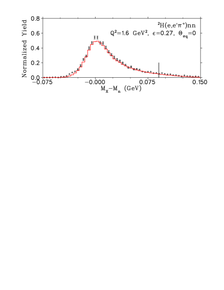
Figure 7: (Color online) Missing mass of the undetected nucleon calculated as quasi-free pion electroproduction for a representative $\pi^{+}$ setting. The diamonds are experimental data, and the red line is the quasi-free Monte Carlo simulation. The vertical line indicates the $M_{X}$ cut upper limit.

In extracting the deuterium cross sections, it is desirable to keep as much of the missing-mass tail as possible (up to the two-pion threshold of 1.1 GeV), to maximize the acceptance of the “quasifree” distribution, and to minimize the systematic uncertainty associated with the missing mass cut.

The thick collimators of the HMS and SOS are very effective at stopping electrons, but a non-negligible fraction of the pions undergo multiple scattering and ionization energy loss and consequentially end up contributing to the experimental yield Gaskellthesis . These pion (hadron) punch-through events have been observed in earlier experiments, and corrections are needed for a precise yield extraction. Since the pions in F_π-1 and F_π-2 are detected in the HMS, the implementation of the simulated collimator punch-through events was done for only this arm. The HMS event simulation therefore takes into account the probability that a pion interacts hadronically with the collimator (allowing the pion to undergo multiple scattering and ionization energy loss). After implementing the pion punch-through events in SIMC, the $M_{X}$ cut upper limit was determined by the value where the missing mass peak is no longer well reproduced by a quasi-free Monte Carlo simulation including all known detector effects, indicating the presence of additional backgrounds, such as two pion production. The missing mass cut was taken to be 0.875$\leq M_{X}\leq$1.03 GeV. It is wider than the one used in the analysis of the hydrogen data because of Fermi motion in the deuteron. Compared to hydrogen, the backgrounds from target windows and random coincidences are generally larger due to the wider $M_{X}$ cut.

III.3 Determination of Separated Structure Functions

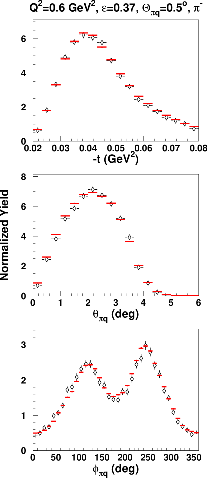
Figure 8: (Color online) Normalized experimental $\pi^{-}$ yield (black diamonds) in comparison to the quasi-free Monte Carlo simulation (red lines) for one HMS+SOS setting at $Q^{2}$=0.60 GeV², low $\epsilon$.

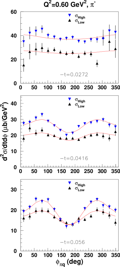
Figure 9: (Color online) Unseparated experimental $\pi^{-}$ cross sections as a function of azimuthal angle $\phi$ at $Q^{2}$=0.60 GeV², low $\epsilon$ (black triangles) and high $\epsilon$ (blue inverted triangles). The curves shown represent the fit of the measured values of the cross section to Eqn. III.1. In this fit, all four parameters $\sigma_{L,T,LT,TT}$ are extracted simultaneously, separate for each $-t$ bin.

The SIMC model cross section and the final separated structure functions were determined in the same (iterative) procedure. The model cross section was taken as the product of a global function describing the $W$-dependence times (a sum of) $Q^{2}$ and $t$ dependent functions for the different structure functions. For the $LT$ and $TT$ parts, their leading order dependence on $\sin$($\theta_{CM}$) was taken into account raskin . The $W$-dependence was taken as $(W^{2}-M_{N}^{2})^{-2}$, where $M_{N}$ is the struck nucleon mass, based on analyses of experimental data from Refs. Brauel1 ; beb78 . For the parts depending on $Q^{2}$ and $t$, phenomenological forms were used and the parameters were fitted. For all $t$-bins at every (central) $Q^{2}$ setting, $\phi$-dependent cross sections were determined both at high and low $\epsilon$ for chosen values of $\overline{W}$, $\overline{Q}^{2}$ (and corresponding values of $\theta_{\pi}$ and $\epsilon$) according to Eqn. 7. The iteration procedure was repeated until satisfactory agreement between the experimental and simulated distributions was obtained, the values of $\sigma_{L,T,LT,TT}$ (and the associated fit parameters) were stable in subsequent iterations, and the parameters fitted at the individual $Q^{2}$-settings did not change much with $Q^{2}$. A representative example of some relevant variables and of the fit of the experimental cross section as a function of $\phi_{\pi}$ is shown in Figs. 8, 9. The cosine structure from the interference terms is clearly visible in Fig. 9.

This procedure was carried out independently for $\pi^{+}$ and $\pi^{-}$ at each $Q^{2}$, in order to have optimal descriptions in the different kinematic ranges covered. The parameterizations used in the F_π-1 $\pi^{+}$ analysis are:

$$\frac{d\sigma_{L}}{dt} = g(W)\bigl{(}p_{1}+p_{2}\ln(Q^{2})\bigr{)}e^{(p_{3}+p_{4}\ln(Q^{2}))(-t)},$$

$$\frac{d\sigma_{T}}{dt} = g(W)\biggl{(}\frac{|t|-|t_{\text{ave}}|}{|t_{\text{ave}}|}\biggr{)}$$

$$\times \biggl{(}p_{5}+p_{6}\ln(Q^{2})+\bigl{(}p_{7}+p_{8}\ln(Q^{2})\bigr{)}\biggr{)},$$

$$\frac{d\sigma_{LT}}{dt} = g(W)p_{9}e^{p_{10}(-t)}\sin\theta_{\text{CM}},$$ (9)

$$\frac{d\sigma_{TT}}{dt} = g(W)f(t)\frac{p_{11}}{Q^{2}}e^{-Q^{2}}\sin^{2}\theta_{\text{CM}},$$

where $g(W)=1/(W^{2}-m_{p}^{2})^{2}$ is the assumed $W$-dependence discussed earlier, $f(t)=-t/(-t-m_{\pi}^{2})^{2}$ is the pion pole factor, $|t_{\text{ave}}|$ is the average $-t$ value for a given kinematic setting, given by $|t_{\text{ave}}|=(0.105+0.04\ln(Q^{2}))Q^{2}$, and $p_{i=1,...,12}$ are the fit parameters.

For the F_π-1 $\pi^{-}$ analysis, a slightly different parameterization (because $\sigma_{T}$ and $\sigma_{TT}$ showed a stronger $Q^{2}$-dependence) yielded a better fit:

$$\frac{d\sigma_{L}}{dt} = g(W)\bigl{(}p_{1}+p_{2}\ln(Q^{2})\bigr{)}e^{(p_{3}+p_{4}\ln(Q^{2}))(-t)},$$

$$\frac{d\sigma_{T}}{dt} = g(W)\biggl{(}p_{5}+\frac{p_{6}}{Q^{4}+0.1}$$

$$+ \bigl{(}p_{7}+p_{8}\ln(Q^{2})\bigr{)}\biggl{(}\frac{|t|-|t_{\text{ave}}|}{|t_{\text{ave}}|}\biggr{)}\biggr{)},$$

$$\frac{d\sigma_{LT}}{dt} = g(W)p_{9}e^{p_{10}(-t)}\sin\theta_{\text{CM}},$$ (10)

$$\frac{d\sigma_{TT}}{dt} = g(W)f(t)\biggl{(}\frac{p_{11}}{Q^{2}}+\frac{p_{12}}{Q^{4}+0.2}\biggr{)}\sin^{2}\theta_{\text{CM}}.$$

In the F_π-2 analyses, a common parameterization (similar to those in F_π-1) was used for both $\pi^{+}$ and $\pi^{-}$:

$$\frac{d\sigma_{L}}{dt} = g(W)\bigl{(}p_{1}+p_{2}\ln(Q^{2})\bigr{)}e^{(p_{3}+p_{4}\ln(Q^{2}))(-t-0.2)},$$

$$\frac{d\sigma_{T}}{dt} = g(W)\biggl{(}p_{5}+p_{6}\ln(Q^{2})$$

$$+ \bigl{(}p_{7}+p_{8}\ln(Q^{2})\bigr{)}\biggl{(}\frac{|t|-|t_{\text{ave}}|}{|t_{\text{ave}}|}\biggr{)}\biggr{)},$$

$$\frac{d\sigma_{LT}}{dt} = g(W)\biggl{(}p_{9}e^{p_{10}(-t)}+\frac{p_{11}}{(-t)}\biggr{)}\sin\theta_{\text{CM}},$$ (11)

$$\frac{d\sigma_{TT}}{dt} = g(W)f(t)\frac{p_{12}}{Q^{2}}e^{-Q^{2}}\sin^{2}\theta_{\text{CM}},$$

where $|t_{\text{ave}}|=\bigl{(}0.0735+0.028\ln(Q^{2})\bigr{)}Q^{2}$ and $p_{4}=0$.

Correction	Uncorrelated	$\epsilon$ uncorr.	Correlated
	(pt-to-pt)	t corr.	(scale)
	[%]	[%]	[%]
d$\theta_{e}$	0.1	0.7-1.1
d$E_{\text{beam}}$	0.1	0.2-0.3
d$P_{e}$	0.1	0.1-0.3
d$\theta_{\pi}$	0.1	0.2-0.3
Radiative corr		0.4	2.0
HMS $\beta$ corr	0.4
Particle ID		0.2
Pion absorption			1.0
Pion decay	0.03		1.0
HMS Tracking ($\pi^{+}$)		0.4	1.0
HMS Tracking ($\pi^{-}$)		1.3	1.0
SOS Tracking		0.2	0.5
Charge		0.3	0.5
Target Thickness		0.3	1.0
CPU dead time		0.2
HMS Trigger		0.1
SOS Trigger		0.1
Electronic DT		0.1
HMS Cer. block. ($\pi^{-}$)	0.7		1.0
Acceptance	1.0	0.6	1.0
Total ($\pi^{+}$)	1.1	1.3-1.6	3.1
Total ($\pi^{-}$)	1.3	1.8-2.0	3.2

Table 3: Systematic uncertainties for F_π-1. Those items not discussed explicitly in preceeding sections are assumed to be the same as for the published ¹H analysis. These are the uncertainties in: kinematic offsets, radiative corrections, pion decay, SOS tracking, trigger efficiency, CPU and electronic dead time, and acceptance. The systematic uncertainties in each column are added quadratically to obtain the total systematic uncertainty.

Correction	Uncorrelated	$\epsilon$ uncorr.	Correlated
	(pt-to-pt)	t corr.	(scale)
	[%]	[%]	[%]
d$\theta_{e}$	0.1	0.7-1.1
d$E_{\text{beam}}$	0.1	0.2-0.3
d$P_{e}$	0.1	0.1-0.3
d$\theta_{\pi}$	0.1	0.2-0.3
Radiative corr		0.4	2.0
HMS $\beta$ corr ($\pi^{+}$)	0.12
HMS $\beta$ corr ($\pi^{-}$)	0.18
Particle ID		0.2
Pion absorption			1.0
Pion decay	0.03		1.0
HMS Tracking ($\pi^{+}$)		0.3	0.5
HMS Tracking ($\pi^{-}$)		0.45	0.75
SOS Tracking		0.2	0.5
Charge		0.3	0.5
Target Thickness		0.2	0.8
CPU dead time		0.2
HMS Trigger		0.1
SOS Trigger		0.1
Electronic DT		0.1
HMS Cer. block. ($\pi^{-}$)	0.3		0.8
Acceptance	0.6	0.6	1.0
Total ($\pi^{+}$)	0.6	1.2-1.5	2.9
Total ($\pi^{-}$)	0.7	1.3-1.6	3.1

Table 4: Systematic uncertainties for F_π-2, similar to Table 3. Those items not discussed explicitly in preceeding sections are assumed to be the same as for the published ¹H analysis.

III.4 Systematic Uncertainties due to Missing Mass Cut and SIMC Model Dependence

Since the extracted separated cross sections depend in principle on the cross section model, there is a “model systematic uncertainty.” This uncertainty was studied by extracting $\sigma_{L}$ and $\sigma_{T}$ with different cross section models. There is a second, related uncertainty due to the modeling of the missing mass distribution. The combined systematic uncertainty due to both effects was estimated by modifying the missing mass cuts and SIMC model parameters $p_{i}$ and investigating the resulting differences on the separated cross sections.

To estimate the missing mass cut dependence, the experimental and simulated data were analyzed with two tighter missing mass cuts, $M_{X}<0.98,\ 1.00$ GeV. A detailed comparison of the separated cross sections for each $t$-bin indicated that the $\pi^{-}$ separated cross sections for higher $-t$ at $Q^{2}$=0.6, 1.0 GeV² $\sigma_{L}$ were extremely sensitive to the applied $M_{X}$ cut and/or the disabling of the collimator pion punch-through routine in the SIMC simulations. We believe this is a result of the incomplete $\phi$ coverage for these settings, as listed in Table 1. The data for any $\pi^{-}$ $t$-bin were discarded if $\sigma_{L}$ changed significantly more than the statistical uncertainty when the nominal $M_{X}<$1.03 GeV cut is replaced with a $M_{X}<$1.00 GeV cut in both the experimental and simulation analyses. For the remaining $\pi^{+}$ and $\pi^{-}$ data, the differences between the “final” separated cross sections and those determined with tighter $M_{X}$ cuts were computed and the standard deviation was tabulated for each $-t$ bin at each $Q^{2}$. These standard deviations for the remaining F_π-1 $\pi^{-}$ data are in almost all cases larger than for the corresponding $\pi^{+}$ data, generally comparable to the statistical errors. The standard deviations are typically smallest at or near $-t_{\text{min}}$ and grow with increasing $-t$.

The cross section model dependence was estimated in a similar manner. Since the longitudinal and transverse cross sections in the model reproduce the experimental values to within 10%, these two terms were independently increased and decreased by 10% in the model. Independent of this, the separated cross sections were also determined by alternately setting $\sigma_{LT}$=0 and $\sigma_{TT}$=0 in the model. Unseparated cross sections were calculated using Eqn. 7 and a fit performed using Eqn. III.1 to extract $L$/$T$/$LT$/$TT$. The differences between the “final” separated cross sections minus the six independent variations were computed and the standard deviations tabulated for each $-t$ bin at each $Q^{2}$ in the same manner as the missing mass cut study. The model sensitivities of the $L$,$T$ cross sections are generally similar to each other, and exhibit a weaker $t$-dependence than the $M_{X}$ cut sensitivities. The observed variations are relatively small, about half the statistical uncertainties in these cross sections (per $t$-bin) of 5-10%. The reason is that $\sigma_{L}$ and $\sigma_{T}$ are effectively determined by the $\phi$-integrated cross section, which reduces the model uncertainty.

The sensitivities of the $TT$ interference response functions are strongly $t$-dependent, being smaller for the lowest $-t$ bins at each $Q^{2}$ and increasing for the larger $-t$ bins. These higher $-t$ bins have relatively poorer statistics as well as incomplete $\phi$ coverage at low $\epsilon$ (as well as at high $\epsilon$ for $\pi^{-}$ $Q^{2}$=0.6, 1.0 GeV²). The $LT$ model sensitivities are smaller than for $TT$, and show no obvious trends.

The standard deviations for each $Q^{2}$, $t$ bin from the two above studies were combined in quadrature to obtain the combined systematic uncertainty due to the missing mass cut and SIMC model dependence (labeled henceforth as “model-dependence” for brevity). The uncertainties computed in this manner are shown as error bands, presented along with the data in Sec. IV, and the values for each bin are listed as the second uncertainty in Tables 5, 6.

III.5 Systematic Uncertainties

The various systematic uncertainties determined in Secs. II,  III are listed in Tables 3, 4. Those items not discussed explicitly in these sections are assumed to be the same as for the previously published ¹H analyses. The systematic uncertainties are subdivided into correlated and uncorrelated contributions. The correlated uncertainties, i.e., those that are the same for both $\epsilon$ points, such as target thickness corrections, are attributed directly to the separated cross sections. Uncorrelated uncertainties are attributed to the unseparated cross sections, with the result that in the separation of $\sigma_{L}$ and $\sigma_{T}$ they are inflated, just as the statistical uncertainties, by the factor $1/\Delta\epsilon$ (for $\sigma_{L}$), which is about three. The uncorrelated uncertainties can be further subdivided into those that differ in size between $\epsilon$ points, but may influence the $t$-dependence at a fixed value of $\epsilon$ in a correlated way. The largest contributions to the “$t$-correlated” uncertainty are acceptance and kinematic offsets, and as a result, they are the dominating systematic uncertainties for, e.g. $\sigma_{L}$. In addition to the uncertainties listed below, are the uncertainties in the separated cross sections at each $-t$, $Q^{2}$ setting due to the $M_{X}$ cut and SIMC model “model-dependence”.

IV Results and Discussion

IV.1 ²H$\bf(e,e^{\prime}\pi^{\pm})NN_{s}$ Separated Cross Sections and Ratios

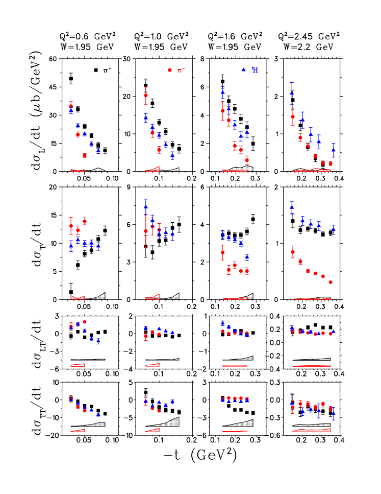
Figure 10: (Color online) Separated cross sections as a function of $-t$. $\pi^{-}$ from ²H: [red circles], $\pi^{+}$ from ²H: [black squares], $\pi^{+}$ from ¹H: [blue triangles]. The error bars include both statistical and uncorrelated systematic uncertainties. The “model-dependences” of the $L$, $T$, $LT$, $TT$ cross sections are indicated by the shaded bands, by which all data points move collectively. The ¹H data have not been scaled to the mean $\overline{Q^{2}}$, $\overline{W}$ values for each $-t$ bin of ²H data. In addition, please keep in mind the issues relating to ²H off-shell effects before directly comparing the ¹H and ²H data.

$\overline{W}$	$\overline{Q^{2}}$	$-t$	$\sigma_{T}$	$\sigma_{L}$	$\sigma_{TT}$	$\sigma_{LT}$
(GeV)	(GeV2)	(GeV2)	($\mu$b/GeV2)	($\mu$b/GeV2)	($\mu$b/GeV2)	($\mu$b/GeV2)
2H$(e,e^{\prime}\pi^{-})pp_{s}$
$Q^{2}=0.60$ GeV2 $W=1.95$ GeV
1.9733	0.5505	0.026	13.07 $\pm$ 1.44 $\pm$ 0.69	34.74 $\pm$ 2.39 $\pm$ 1.03	0.47 $\pm$ 1.17 $\pm$ 0.13	1.19 $\pm$ 0.70 $\pm$ 0.26
1.9568	0.5765	0.038	12.31 $\pm$ 0.69 $\pm$ 0.17	19.71 $\pm$ 1.13 $\pm$ 0.36	-3.95 $\pm$ 0.48 $\pm$ 0.74	1.54 $\pm$ 0.24 $\pm$ 0.42
1.9452	0.6048	0.050	13.88 $\pm$ 0.62 $\pm$ 0.66	8.53 $\pm$ 1.03 $\pm$ 1.01	-6.13 $\pm$ 0.43 $\pm$ 1.44	2.00 $\pm$ 0.20 $\pm$ 0.48
$Q^{2}=1.00$ GeV2 $W=1.95$ GeV
1.9864	0.9095	0.060	5.47 $\pm$ 1.29 $\pm$ 0.17	20.25 $\pm$ 2.25 $\pm$ 0.29	-0.50 $\pm$ 0.80 $\pm$ 0.06	-0.30 $\pm$ 0.48 $\pm$ 0.12
1.9703	0.9483	0.080	5.85 $\pm$ 0.68 $\pm$ 0.16	10.27 $\pm$ 1.16 $\pm$ 0.47	-2.31 $\pm$ 0.38 $\pm$ 0.50	0.16 $\pm$ 0.19 $\pm$ 0.19
1.9489	0.9977	0.100	5.56 $\pm$ 0.51 $\pm$ 0.46	5.75 $\pm$ 0.91 $\pm$ 1.31	-3.09 $\pm$ 0.32 $\pm$ 1.01	-0.08 $\pm$ 0.15 $\pm$ 0.33
$Q^{2}=1.60$ GeV2 $W=1.95$ GeV
2.0116	1.4345	0.135	2.51 $\pm$ 0.39 $\pm$ 0.02	4.31 $\pm$ 0.66 $\pm$ 0.12	0.22 $\pm$ 0.16 $\pm$ 0.04	0.13 $\pm$ 0.07 $\pm$ 0.03
1.9867	1.5064	0.165	1.58 $\pm$ 0.24 $\pm$ 0.08	3.64 $\pm$ 0.40 $\pm$ 0.09	0.33 $\pm$ 0.10 $\pm$ 0.04	-0.00 $\pm$ 0.05 $\pm$ 0.02
1.9644	1.5650	0.195	1.83 $\pm$ 0.18 $\pm$ 0.05	1.82 $\pm$ 0.30 $\pm$ 0.05	0.25 $\pm$ 0.08 $\pm$ 0.05	0.04 $\pm$ 0.04 $\pm$ 0.03
1.9433	1.6178	0.225	1.52 $\pm$ 0.16 $\pm$ 0.10	1.53 $\pm$ 0.27 $\pm$ 0.11	0.29 $\pm$ 0.08 $\pm$ 0.09	0.04 $\pm$ 0.03 $\pm$ 0.03
1.9229	1.6664	0.255	1.52 $\pm$ 0.18 $\pm$ 0.15	0.80 $\pm$ 0.29 $\pm$ 0.10	0.19 $\pm$ 0.09 $\pm$ 0.16	0.03 $\pm$ 0.03 $\pm$ 0.03
$Q^{2}=2.45$ GeV2 $W=2.22$ GeV
2.2978	2.1619	0.150	0.85 $\pm$ 0.11 $\pm$ 0.01	1.46 $\pm$ 0.22 $\pm$ 0.02	-0.13 $\pm$ 0.10 $\pm$ 0.01	0.18 $\pm$ 0.04 $\pm$ 0.01
2.2695	2.2598	0.190	0.67 $\pm$ 0.05 $\pm$ 0.01	0.90 $\pm$ 0.10 $\pm$ 0.04	-0.07 $\pm$ 0.05 $\pm$ 0.05	0.16 $\pm$ 0.03 $\pm$ 0.01
2.2400	2.3537	0.230	0.51 $\pm$ 0.03 $\pm$ 0.02	0.67 $\pm$ 0.07 $\pm$ 0.01	-0.07 $\pm$ 0.04 $\pm$ 0.03	0.15 $\pm$ 0.02 $\pm$ 0.02
2.2154	2.4289	0.270	0.47 $\pm$ 0.03 $\pm$ 0.01	0.39 $\pm$ 0.06 $\pm$ 0.08	-0.13 $\pm$ 0.04 $\pm$ 0.03	0.13 $\pm$ 0.02 $\pm$ 0.02
2.1932	2.4993	0.310	0.41 $\pm$ 0.02 $\pm$ 0.01	0.22 $\pm$ 0.06 $\pm$ 0.06	-0.07 $\pm$ 0.03 $\pm$ 0.04	0.14 $\pm$ 0.02 $\pm$ 0.02
2.1688	2.5753	0.350	0.31 $\pm$ 0.02 $\pm$ 0.03	0.21 $\pm$ 0.06 $\pm$ 0.04	-0.15 $\pm$ 0.03 $\pm$ 0.06	0.13 $\pm$ 0.02 $\pm$ 0.02

Table 5: Separated cross sections for the ²H$(e,e^{\prime}\pi^{-})pp_{s}$ reaction. The first uncertainties listed are statistical only. The second uncertainties listed are the $M_{X}$ cut and SIMC model “model-dependences”. In addition to these, the systematic uncertainties listed in Tables 3 and 4 must be applied.

$\overline{W}$	$\overline{Q^{2}}$	$-t$	$\sigma_{T}$	$\sigma_{L}$	$\sigma_{TT}$	$\sigma_{LT}$
(GeV)	(GeV2)	(GeV2)	($\mu$b/GeV2)	($\mu$b/GeV2)	($\mu$b/GeV2)	($\mu$b/GeV2)
2H$(e,e^{\prime}\pi^{+})nn_{s}$
$Q^{2}=0.60$ GeV2 $W=1.95$ GeV
1.9702	0.5445	0.026	1.32 $\pm$ 1.49 $\pm$ 0.10	49.44 $\pm$ 2.51 $\pm$ 0.56	0.80 $\pm$ 1.11 $\pm$ 0.21	-0.40 $\pm$ 0.53 $\pm$ 0.08
1.9572	0.5736	0.038	6.15 $\pm$ 0.64 $\pm$ 0.06	33.17 $\pm$ 1.18 $\pm$ 0.16	-1.06 $\pm$ 0.56 $\pm$ 0.24	0.32 $\pm$ 0.26 $\pm$ 0.07
1.9495	0.5953	0.050	8.15 $\pm$ 0.51 $\pm$ 0.12	23.94 $\pm$ 0.97 $\pm$ 0.47	-3.33 $\pm$ 0.46 $\pm$ 0.65	-0.61 $\pm$ 0.20 $\pm$ 0.10
1.9444	0.6092	0.062	8.76 $\pm$ 0.54 $\pm$ 0.17	19.08 $\pm$ 0.99 $\pm$ 0.54	-3.73 $\pm$ 0.49 $\pm$ 1.02	-0.25 $\pm$ 0.21 $\pm$ 0.11
1.9423	0.6146	0.074	10.73 $\pm$ 0.64 $\pm$ 0.48	14.08 $\pm$ 1.15 $\pm$ 1.90	-5.99 $\pm$ 0.61 $\pm$ 2.04	0.19 $\pm$ 0.23 $\pm$ 0.17
1.9411	0.6206	0.086	12.25 $\pm$ 0.81 $\pm$ 1.29	11.18 $\pm$ 1.45 $\pm$ 0.53	-7.84 $\pm$ 0.83 $\pm$ 2.19	0.30 $\pm$ 0.29 $\pm$ 0.18
$Q^{2}=0.75$ GeV2 $W=1.95$ GeV
1.9894	0.6668	0.037	8.76 $\pm$ 1.22 $\pm$ 0.15	21.76 $\pm$ 2.03 $\pm$ 0.48	2.13 $\pm$ 0.68 $\pm$ 0.18	0.67 $\pm$ 0.29 $\pm$ 0.02
1.9691	0.6978	0.051	10.82 $\pm$ 0.80 $\pm$ 0.29	15.90 $\pm$ 1.32 $\pm$ 0.39	-0.54 $\pm$ 0.42 $\pm$ 0.38	0.42 $\pm$ 0.18 $\pm$ 0.07
1.9579	0.7259	0.065	10.34 $\pm$ 0.66 $\pm$ 0.34	14.41 $\pm$ 1.11 $\pm$ 0.28	-3.70 $\pm$ 0.38 $\pm$ 0.75	0.54 $\pm$ 0.15 $\pm$ 0.10
1.9467	0.7483	0.079	9.36 $\pm$ 0.64 $\pm$ 0.29	16.06 $\pm$ 1.08 $\pm$ 1.65	-6.93 $\pm$ 0.42 $\pm$ 1.42	0.22 $\pm$ 0.13 $\pm$ 0.11
1.9404	0.7640	0.093	9.75 $\pm$ 0.69 $\pm$ 0.37	15.82 $\pm$ 1.18 $\pm$ 4.73	-9.57 $\pm$ 0.52 $\pm$ 2.41	0.39 $\pm$ 0.15 $\pm$ 0.23
1.9357	0.7805	0.107	11.10 $\pm$ 0.81 $\pm$ 0.58	13.76 $\pm$ 1.38 $\pm$ 7.22	-12.50 $\pm$ 0.69 $\pm$ 3.45	1.12 $\pm$ 0.16 $\pm$ 0.41
$Q^{2}=1.00$ GeV2 $W=1.95$ GeV
1.9970	0.8941	0.060	4.24 $\pm$ 0.82 $\pm$ 0.06	22.87 $\pm$ 1.55 $\pm$ 0.28	2.13 $\pm$ 0.71 $\pm$ 0.08	0.17 $\pm$ 0.31 $\pm$ 0.04
1.9802	0.9305	0.080	3.78 $\pm$ 0.50 $\pm$ 0.05	18.16 $\pm$ 0.95 $\pm$ 0.12	-0.42 $\pm$ 0.41 $\pm$ 0.31	-0.25 $\pm$ 0.18 $\pm$ 0.04
1.9602	0.9745	0.100	4.68 $\pm$ 0.40 $\pm$ 0.14	13.00 $\pm$ 0.76 $\pm$ 0.45	-2.07 $\pm$ 0.35 $\pm$ 0.59	-0.23 $\pm$ 0.13 $\pm$ 0.06
1.9458	1.0061	0.120	4.74 $\pm$ 0.37 $\pm$ 0.09	10.60 $\pm$ 0.72 $\pm$ 0.20	-2.93 $\pm$ 0.36 $\pm$ 1.01	-0.20 $\pm$ 0.12 $\pm$ 0.06
1.9349	1.0320	0.140	5.72 $\pm$ 0.44 $\pm$ 0.20	7.10 $\pm$ 0.83 $\pm$ 0.45	-3.07 $\pm$ 0.43 $\pm$ 2.03	-0.36 $\pm$ 0.13 $\pm$ 0.05
1.9247	1.0602	0.160	6.00 $\pm$ 0.62 $\pm$ 0.55	6.04 $\pm$ 1.14 $\pm$ 1.05	-3.44 $\pm$ 0.58 $\pm$ 2.69	-0.22 $\pm$ 0.16 $\pm$ 0.21
$Q^{2}=1.60$ GeV2 $W=1.95$ GeV
2.0112	1.4353	0.135	3.43 $\pm$ 0.22 $\pm$ 0.03	6.38 $\pm$ 0.43 $\pm$ 0.03	0.34 $\pm$ 0.22 $\pm$ 0.09	-0.05 $\pm$ 0.09 $\pm$ 0.01
1.9884	1.4998	0.165	3.52 $\pm$ 0.17 $\pm$ 0.07	5.00 $\pm$ 0.34 $\pm$ 0.12	-1.01 $\pm$ 0.16 $\pm$ 0.23	-0.03 $\pm$ 0.06 $\pm$ 0.02
1.9669	1.5553	0.195	3.43 $\pm$ 0.15 $\pm$ 0.05	4.44 $\pm$ 0.30 $\pm$ 0.31	-1.70 $\pm$ 0.16 $\pm$ 0.44	0.16 $\pm$ 0.05 $\pm$ 0.05
1.9463	1.6082	0.225	3.44 $\pm$ 0.15 $\pm$ 0.12	3.74 $\pm$ 0.30 $\pm$ 0.26	-1.70 $\pm$ 0.17 $\pm$ 0.65	0.16 $\pm$ 0.05 $\pm$ 0.06
1.9276	1.6568	0.255	3.63 $\pm$ 0.18 $\pm$ 0.18	3.15 $\pm$ 0.36 $\pm$ 0.43	-2.10 $\pm$ 0.20 $\pm$ 0.86	-0.02 $\pm$ 0.05 $\pm$ 0.13
1.9097	1.7025	0.285	4.29 $\pm$ 0.25 $\pm$ 0.36	1.97 $\pm$ 0.48 $\pm$ 0.30	-2.24 $\pm$ 0.26 $\pm$ 1.20	0.04 $\pm$ 0.07 $\pm$ 0.25
$Q^{2}=2.45$ GeV2 $W=2.22$ GeV
2.3017	2.1503	0.150	1.40 $\pm$ 0.12 $\pm$ 0.01	1.90 $\pm$ 0.26 $\pm$ 0.03	-0.04 $\pm$ 0.12 $\pm$ 0.02	0.15 $\pm$ 0.05 $\pm$ 0.01
2.2719	2.2518	0.190	1.23 $\pm$ 0.06 $\pm$ 0.02	1.22 $\pm$ 0.14 $\pm$ 0.08	-0.21 $\pm$ 0.07 $\pm$ 0.04	0.18 $\pm$ 0.03 $\pm$ 0.01
2.2448	2.3391	0.230	1.26 $\pm$ 0.04 $\pm$ 0.01	0.65 $\pm$ 0.11 $\pm$ 0.03	-0.12 $\pm$ 0.06 $\pm$ 0.03	0.23 $\pm$ 0.03 $\pm$ 0.02
2.2197	2.4180	0.270	1.22 $\pm$ 0.04 $\pm$ 0.03	0.35 $\pm$ 0.09 $\pm$ 0.02	-0.16 $\pm$ 0.05 $\pm$ 0.04	0.26 $\pm$ 0.02 $\pm$ 0.02
2.1977	2.4878	0.310	1.16 $\pm$ 0.04 $\pm$ 0.05	0.18 $\pm$ 0.10 $\pm$ 0.06	-0.19 $\pm$ 0.06 $\pm$ 0.05	0.22 $\pm$ 0.02 $\pm$ 0.02
2.1750	2.5570	0.350	1.19 $\pm$ 0.05 $\pm$ 0.04	-0.10 $\pm$ 0.11 $\pm$ 0.04	-0.22 $\pm$ 0.06 $\pm$ 0.05	0.23 $\pm$ 0.02 $\pm$ 0.04

Table 6: Separated cross sections for the ²H$(e,e^{\prime}\pi^{+})nn_{s}$ reaction. The first uncertainties listed are statistical only. The second uncertainties listed are the $M_{X}$ cut and SIMC model “model-dependences”. In addition to these, the systematic uncertainties listed in Tables 3 and 4 must be applied.

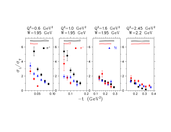
Figure 11: (Color online) $L$/$T$ separated cross section ratios as a function of $-t$ for $\pi^{+}$ [black squares] and $\pi^{-}$ [red circles] production on ²H, and for $\pi^{+}$ on ¹H [blue triangles]. The model-dependences of the ratios are indicated by the shaded bands, by which all data points move collectively.

The $\pi^{\pm}$ separated cross sections from ²H are shown in Fig. 10 and are listed in Tables 5 and 6. Also shown for comparison are our previously published $\pi^{+}$ data from ¹H Blok08 . Please keep in mind the issues relating to ²H off-shell effects discussed in Sec. III.2 before directly comparing the ¹H and ²H data, particularly at higher $-t$, where the effect of Fermi momentum is larger.

In the $L$ response of Fig. 10, the pion pole is evident by the sharp rise at small $-t$. The cross sections for $\pi^{-}$ and $\pi^{+}$ from ²H are similar to each other and to those from ¹H, but there is a general tendency for the $\pi^{-}$ $\sigma_{L}$ to drop more rapidly with $-t$ than the $\pi^{+}$ $\sigma_{L}$.

The $T$ responses are much flatter versus $t$. With the exception of the lowest two $-t$ bins at $Q^{2}$=0.6 GeV², the $\pi^{+}$ $\sigma_{T}$ from ²H are generally within the uncertainties of the $\sigma_{T}$ from ¹H. We have looked very carefully at the analysis of these two low $-t$ bins, but we were unable to identify a specific reason for this behavior, hence we do not believe it is due to an artifact of the analysis. We note that these two $-t$ bins correspond to the smallest relative momentum of the two recoil nucleons in our data set ($<$170 MeV/c), where nucleonic final-state interactions absent for ¹H may be relevant.

It is also seen that the $\pi^{-}$ $\sigma_{T}$ are significantly lower than the $\pi^{+}$ $\sigma_{T}$ at $Q^{2}$=1.6, 2.45 GeV². The suppression of $\sigma_{T}^{\pi^{-}}$ relative to $\sigma_{T}^{\pi^{+}}$ may benefit future measurements of $F_{\pi}(Q^{2})$ since the larger $L$/$T$ ratio in ²H$(e,e^{\prime}\pi^{-})pp_{s}$ would enjoy reduced error magnification compared to $p(e,e^{\prime}\pi^{+})nn_{s}$. This enhancement in the $L$/$T$ ratio at higher $Q^{2}$ is seen more clearly in Fig. 11.

The interference $\sigma_{LT}$, $\sigma_{TT}$ cross sections are shown in the bottom two rows of Fig. 10. Interestingly, at higher $Q^{2}$ the $\pi^{-}$ interference cross sections are more similar to the $\pi^{+}$ cross sections from ¹H than from ²H. Also note that the model-dependence of the interference cross sections grows dramatically with $-t$, particularly for the $\pi^{+}$ cross sections from ²H. The model-dependences from ¹H are not shown, but are significantly smaller.

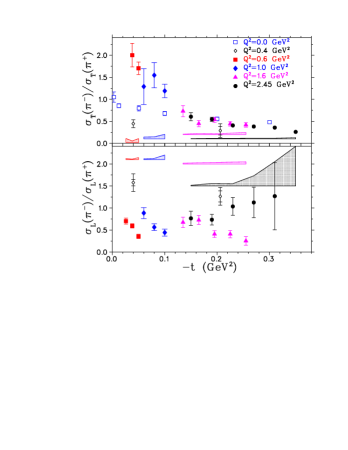
Figure 12: (Color online) The ratios $R_{L}$ and $R_{T}$ versus $-t$ for four $Q^{2}$ settings from this work. The model-dependences of the ratios are indicated by the shaded bands, and the error bars include statistical and uncorrelated systematic uncertainties. Also shown are the ratios at $Q^{2}$=0.4 GeV² in the resonance region from Refs. Gaskellthesis ; Gaskell01 , and $R_{T}$ from the $E_{\gamma}$=3.4 GeV photoproduction data of Ref. heide .

$\pi^{-}/\pi^{+}$ ratios of the separated cross sections were formed, in which nuclear binding and rescattering effects are expected to cancel. (No corrections have been made for electromagnetic FSI or two-photon exchange effects, but these are expected to be small.) Many experimental normalization factors cancel to a high degree in the ratio (acceptance, target thickness, pion decay and absorption in the detectors, radiative corrections, etc.). The principal remaining uncorrelated systematic errors are in the tracking inefficiencies, target boiling corrections (due to different beam currents used), and C̆erenkov blocking corrections.

Figure 12 shows the values of the separated cross section $\pi^{-}/\pi^{+}$ ratios. $R_{L}$ is approximately 0.8 near $-t_{\text{min}}$ at each $Q^{2}$ setting, as predicted in the large $N_{c}$ limit calculation of Ref. frankfurt . Under the not necessarily realistic assumption that the isoscalar and isovector amplitudes are real, $R_{L}=0.8$ gives $A_{S}/A_{V}=6\%$. This is relevant for the extraction of the pion form factor from electroproduction data, which uses a model including some isoscalar background. It is difficult at this stage to make a more quantitative conclusion, but this result is qualitatively in agreement with the findings of our pion form factor analyses Huber08 ; volmer , which found evidence of a small additional contribution to $\sigma_{L}$ not taken into account by the VGL Regge Model in our $Q^{2}$=0.6-1.6 GeV² data at $W=1.95$ GeV, but little evidence for any additional contributions in our $Q^{2}$=1.6-2.45 GeV² data at $W=2.2$ GeV. The main conclusion to be drawn is that pion exchange dominates the forward longitudinal response even $\sim 10\ m_{\pi}^{2}$ away from the pion pole. The $R_{L}$ results from Gaskell, et al. Gaskellthesis ; Gaskell01 at $Q^{2}$=0.4 GeV², $W<1.7$ GeV, are above 1, presumably because of significant resonance contributions.

Also in Fig. 12 are our $R_{T}$ results, following a nearly universal curve with $-t$, and exhibiting only a small $Q^{2}$-dependence. Interestingly, above $-t=0.15$ GeV², the photoproduction $R_{T}$ at $E_{\gamma}$=3.4 GeV from Heide, et al., heide are very close in value to our ratios from electroproduction. Of the $Q^{2}$=0.4 GeV² data from Refs. Gaskellthesis ; Gaskell01 , the higher $-t$ point [$-t=0.21$ GeV² at $W=1.15$ GeV, below the $\Delta_{1232}$] is closer to the ‘universal curve’, while the lower $-t$ point [$-t=0.04$ GeV² at $W=1.6$ GeV, in the resonance region] is well below it.

At the highest $Q^{2}$ and $-t$, $R_{T}$ reaches $0.26\pm 0.02$, which is consistent with the $s$-channel knockout of valence quarks prediction by Nachtmann nachtmann ,

$$\frac{\gamma^{*}_{T}n\rightarrow\pi^{-}p}{\gamma^{*}_{T}p\rightarrow\pi^{+}n}=\Bigl{(}\frac{e_{d}}{e_{u}}\Bigr{)}^{2}=\frac{1}{4},$$ (12)

at sufficiently large $-t$. This value is reached at a much lower value of $-t$ than for the unseparated ratios of Ref. Brauel1 . A value of $-t=0.3$ GeV² seems quite a low value for quark charge scaling arguments to apply directly. This might indicate the partial cancellation of soft QCD corrections in the formation of the $\pi^{-}/\pi^{+}$ ratio. Data at larger $-t$ are needed to see if this interpretation is correct.

Photoproduction data Gao at $-t\geq 3$ GeV² have hinted at quark-partonic behavior, based on the combination of constituent scaling, and experimental results for $R_{T}$. However, the experimental photoproduction cross sections are much larger than can be accounted for by one-hard-gluon-exchange diagrams in a handbag factorization calculation, even at $s\sim 10$ GeV² huang00 . Either the vector meson dominance contribution is still large, or the leading-twist generation of the meson underestimates the handbag contribution kroll02 . However, by forming the $\pi^{-}/\pi^{+}$ ratio the nonperturbative components represented by the form factors and meson distribution amplitude may be divided out, allowing the perturbative contribution to be observed more readily. In the limit that the soft contributions are completely divided out, the one-hard-gluon-exchange calculation predicts kroll02 the simple scaling behavior

$$\frac{d\sigma(\gamma n\rightarrow\pi^{-}p)}{d\sigma(\gamma p\rightarrow\pi^{+}n)}\approx\Bigl{[}\frac{e_{d}(u-m_{p}^{2})+e_{u}(s-m_{p}^{2})}{e_{u}(u-m_{p}^{2})+e_{d}(s-m_{p}^{2})}\Bigr{]}^{2}.$$

The recent JLab data at $\theta_{CM}=90^{o}$ and above $-t=3$ GeV² are in agreement with the above expression, while those at smaller $\theta_{CM}$ are not Gao .

A possible explanation for the relatively early perturbative behavior in transverse electroproduction is that the quasi-free process $eq\rightarrow eq$ has the minimal total number of elementary fields (4) brodsky73 and so requires only a single photon exchange. The fact that only a single pion is created may be crucial to this quasi-free picture, since it implies that the string tension never greatly exceeds O($m_{\pi}$). By contrast, the photoproduction reaction $\gamma q\rightarrow q$ at high $-t$ can only proceed if the initial quark is far off its mass shell. The required strong binding to other quarks leads to the larger number of active elementary fields in $\gamma N\rightarrow\pi N$ (9) and hence $s^{2-n}=s^{-7}$ scaling.

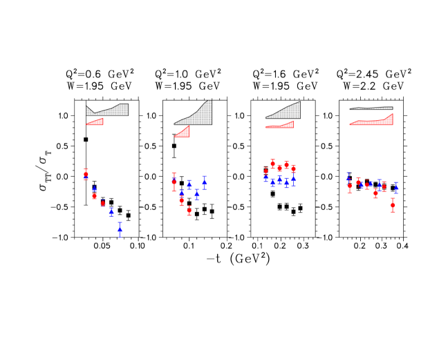
Figure 13: (Color online) $TT$/$T$ separated cross section ratios as a function of $-t$. The legend is the same as in Fig. 11.

Another prediction of the quark-parton mechanism nachtmann is the suppression of $\sigma_{TT}/\sigma_{T}$ due to $s$-channel helicity conservation. Our data support this hypothesis in that $\sigma_{TT}$ decreases more rapidly than $\sigma_{T}$ with increasing $Q^{2}$. This is particularly true for $\pi^{+}$ electroproduction on both ²H and ¹H, where $\sigma_{TT}/\sigma_{T}\simeq(-19\pm 1)\%$ at our highest $Q^{2}$, $-t$ setting (see Fig.  13). The $\sigma_{TT}/\sigma_{T}$ ratios for $\pi^{-}$ production are generally consistent with those for $\pi^{+}$, once one takes into account the respective error bars and model-dependences.

IV.2 Comparison of Various Models with the Data

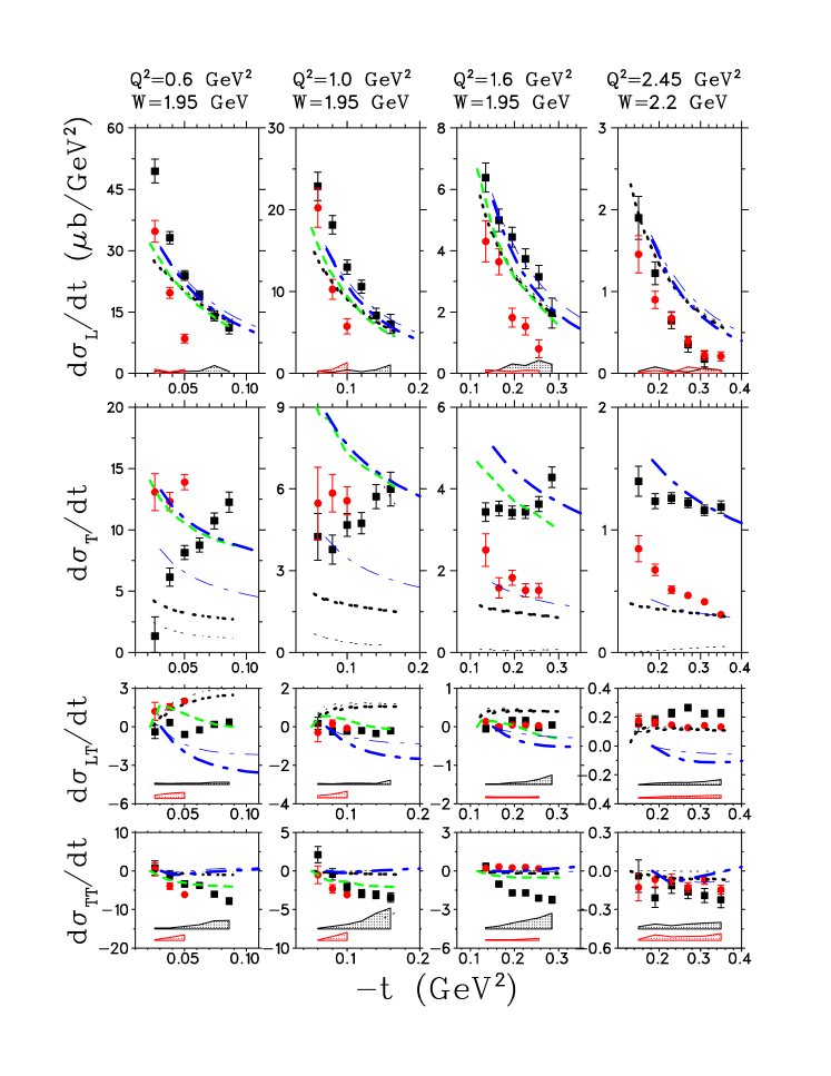
Figure 14: (Color online) Comparison of separated cross sections as a function of $-t$ with various models. $\pi^{-}$ from ²H: [red circles], $\pi^{+}$ from ²H:[black squares]. The data error bars and bands are as in Fig. 10. The dotted black curves are predictions of the VGL Regge model VGL1 using the values $\Lambda_{\pi}^{2}$=0.0.394, 0.411, 0.455, 0.491 GeV² and $\Lambda_{\rho}$=1.50 GeV², as determined from fits to our ¹H data Huber08 . The short-dashed green curves are predictions by Kaskulov and Mosel kaskulov , and the dot-dashed blue curves are the predictions by Vrancx and Ryckebusch vrancx , both models are evaluated at the nominal kinematics. In all cases, the thick lines are the model predictions for $\pi^{+}$ and the thin lines are the predictions for $\pi^{-}$.

Figure 15: (Color online) Comparison of separated cross sections as a function of $-t$ with various models. The symbols are as in Fig. 14. The long-dashed magenta curves are the predictions of the MAID07 model maid07 , and the solid red curves are predictions by Goloskokov and Kroll gk13 . Both models are evaluated at the same $\overline{W}$, $\overline{Q^{2}}$ as the data. The thick lines are the model predictions for $\pi^{+}$ and the thin lines are the predictions for $\pi^{-}$.

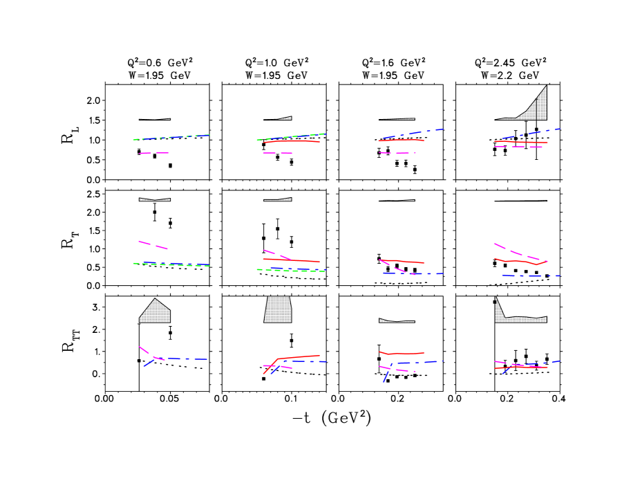
Figure 16: (Color online) The ratios $R_{L}$, $R_{T}$ and $R_{TT}\equiv\sigma_{TT}^{\pi^{-}}/\sigma_{TT}^{\pi^{+}}$ versus $-t$ for four $Q^{2}$ settings. The error bars include statistical and uncorrelated systematic uncertainties. The model-dependences of the ratios are indicated by the shaded bands. The model legend is the same as Figs. 14, 15; i.e. dotted black curves are the VGL Regge model VGL1 , short-dashed green curves are Kaskulov and Mosel kaskulov , dot-dashed blue curves are Vrancx and Ryckebusch vrancx , long-dashed magenta curves are the MAID07 model maid07 , and solid red curves are Goloskokov and Kroll gk13 .

The separated cross section data are compared to a variety of models in Figs. 14, 15, and our $R_{L}$, $R_{T}$ and $R_{TT}\equiv\sigma_{TT}^{\pi^{-}}/\sigma_{TT}^{\pi^{+}}$ ratios are compared to the same models in Fig. 16.

The VGL Regge model, which does well for photoproduction VGL1 and longitudinal electroproduction Blok08 , fails to describe the magnitude or the $Q^{2}$-dependence of $\sigma_{T}$. For any choice for the $\rho\pi\gamma$ monopole mass, it underpredicts the transverse cross sections by a large factor, which increases with $Q^{2}$. As briefly mentioned in the introduction, the VGL Regge model was extended by Kaskulov and Mosel (KM) kaskulov and more recently by Vrancx and Ryckebusch (VR) vrancx . KM add to the Regge model a hadronic model, which incorporates DIS $\pi^{\pm}$ electroproduction at the amplitude level. This DIS process dominates the transverse response at moderate and high $Q^{2}$, increasing the predicted $\sigma_{T}$. In this approach, the residual effects of nucleon resonances in the proton electromagnetic transition form factor are treated as dual to partons, i.e. “resonance-parton (R-P) contributions”. The VR model differs from the KM model by using an alternative R-P transition form factor, which better describes the deep-inelastic $N(e,e^{\prime}\pi^{\pm})$ data.

The VGL model parameters used here are taken from the fits to our ¹H $\sigma_{L}$ data shown in Ref. Huber08 . Similarly, the KM and VR models base their parameterization of the pion electromagnetic form factor upon fits to our ¹H $\sigma_{L}$ data. Not surprisingly, the VGL and KM models predict nearly identical $\sigma_{L}$ in Fig. 14, while the VR values are a bit higher. For $\sigma_{T}$, the KM and VR models are much closer to the experimental values than VGL, but they predict a steeper $t$-dependence than exhibited by the data. Of these three models, KM also provides the best description of the $\pi^{+}$ $\sigma_{LT}$ and $\sigma_{TT}$ data.

The $R_{L}$ predictions of the VGL, KM and VR models are nearly identical at $Q^{2}$=0.6, 1.0 GeV², with some differences becoming apparent at larger $Q^{2}$ and $-t$. With the exception of the highest $-t$ points at $Q^{2}$=2.45 GeV², the models generally predict $R_{L}$ ratios that are too large in comparison to the data. As already discussed, the reason for this discrepancy for the three $Q^{2}$ taken at $W=1.95$ GeV is believed to be a small resonance contribution in the longitudinal channel that is not included in these models. The VGL, KM and VR models also generally underpredict $R_{T}$, particularly at $-t_{\text{min}}$. However, the KM and VR models predict systematically larger $R_{T}$ values than VGL due to the addition of the DIS mechanism to the transverse channel. In fact, the VR model comes quite close to the data at higher $-t$, and $Q^{2}$, validating their improvements to the R-P transition form factor, such as a softer proton Dirac form factor.

The MAID model is a phenomenological fit to pion electroproduction data in the canonical resonance region ($W<2$ GeV). This model incorporates Breit-Wigner fits to nucleon resonances and also includes (unitarized) non-resonant backgrounds. Originally introduced in 1998 maid98 , MAID has undergone incremental improvements. Shown here are the results of the most recent version of the MAID model from 2007 maid07 . For these calculations, we have used the MAID07 standard parameter set, although some parameters (such as relative strengths of resonances, the charged pion form factor, etc.) can be adjusted. Finally, note that we apply the MAID model to some kinematics with $W>2$ GeV. Strictly speaking, the model is not constrained in this regime and the results plotted represent an extrapolation of a calculation fit at lower $W$.

For $\sigma_{L}$, the MAID07 predictions are slightly higher than the VGL, KM and VR models, while the $\sigma_{T}$ predictions are midway between the purely Regge-based VGL and the VGL+DIS KM and VR. In terms of $\pi^{-}/\pi^{+}$ ratios, MAID07 provides by far the best description of $R_{L}$, providing further evidence that the disagreement between the pion-pole dominated models and the $R_{L}$ data is due to small resonant contributions in the longitudinal channel. MAID07 also provides a fairly good description of $R_{T}$ at $Q^{2}$=1.6 GeV², although it undershoots the $R_{T}$ at $Q^{2}$=0.6, 1.0 GeV². The overshoot at $Q^{2}$=2.45 GeV² is probably due to the significant extrapolation from the optimized parameter region $W<2$ GeV.

We further investigated the impact of resonances in the MAID07 model on the $\pi^{-}/\pi^{+}$ ratios. With all resonances turned off (Born term and meson exchange contributions on), the model gives $R_{L}\approx 1$ and $R_{T}$ far below the data ($R_{T}\approx$0.5 at $Q^{2}$=0.6, 1.0 GeV², $R_{T}\approx$0.2 at $Q^{2}$=1.6, 2.45 GeV²). Even though the data are acquired near $W=2$ GeV or higher, turning on only the P₃₃(1232) resonance has a significant effect on $R_{T}$ (increasing it to $\approx$1.5 at $Q^{2}$=0.6, 1.0 GeV², and $\approx$0.8 at $Q^{2}$=1.6, 2.45 GeV²), but it has only a small effect on $R_{L}$. Progressively turning on the other resonances yields no clear trend in the behavior of either ratio. Curiously, turning off only the highest three resonances, F₃₇(1950), P₃₁(1910), F₃₅(1905), results in virtually no change from the nominal case. In summary, no clear single resonance seems to account for the global behavior of the separated ratios in the MAID07 model. It would be extremely interesting to see the result if the model parameters could be optimized for higher $W$.

The Goloskokov-Kroll (GK) GPD-based model gk10 ; gk13 is a modified perturbative approach, incorporating the full pion electromagnetic form factor (as determined by fits to our $F_{\pi}$ data Huber08 ) in the longitudinal channel and the $H_{T}$ transversity GPD dominating the transverse channel. The GK model is in good agreement with our $R_{T}$ data at $-t_{\text{min}}$, but predicts too-flat of a $t$-dependence. The predictions for $R_{L}$ are very similar to the pion-pole dominated VGL, KM and VR models.

It is extremely important to keep in mind that the parameters in the GK model are optimized for small skewness ($\xi<0.1$) and large $W>4$ GeV, and have not been adjusted at all for the kinematics of our data. This limitation becomes apparent when comparing the GK-predicted $\sigma_{L}$ and $\sigma_{T}$ to our data in Fig. 15. The predicted $\sigma_{T}$ are too large in magnitude, being entirely off the plotting scale at $Q^{2}$=1.0 GeV², and dropping very rapidly with $-t$ to come close to the data for the highest $-t$ at $Q^{2}$=1.6, 2.45 GeV². The predicted $\sigma_{L}$ are generally similar to, but slightly smaller in magnitude than the VGL, KM and VR models. All four models use our ¹H $\pi^{+}$ data as a constraint in one manner or other. The reasonable agreement between the GPD-based model and our data is sufficiently encouraging in our view to justify further effort to better describe the larger $\xi$, smaller $W$ regime such as covered by our data.

V Summary

We present $L$/$T$/$LT$/$TT$ separated cross sections for the ²H$(e,e^{\prime}\pi^{\pm})NN_{s}$ reactions, at $Q^{2}$=0.6-1.6 GeV², $W=1.95$ GeV and $Q^{2}$=2.45 GeV², $W=2.2$ GeV. The data were acquired with the HMS+SOS spectrometers in Hall C of Jefferson Lab, with the exclusive production of a single pion assured via a missing mass cut. The separated cross sections have typical statistical uncertainties per $t$-bin of 5-10%. The dominant systematic uncertainties are due to HMS tracking at high rates ($\pi^{-}$), HMS C̆erenkov blocking ($\pi^{-}$), cryotarget boiling at high current ($\pi^{+}$), spectrometer acceptance modeling, radiative corrections, pion absorption and decay. These data represent a substantial advance over previous measurements, which were either unseparated at $Q^{2}$=0.7 GeV² Brauel1 , or separated but over a limited kinematic range in the resonance region Gaskell01 ; Gaskellthesis .

In comparison to our previously published $\pi^{+}$ data from ¹H Blok08 , the $\pi^{+}$ $L$/$T$ ratios from ²H are higher at $Q^{2}$=0.6, 1.0 GeV² but fall more steeply with $-t$, are nearly the same as from ¹H at $Q^{2}$=1.6 GeV², and lower at $Q^{2}$=2.45 GeV². In contrast, the $\pi^{-}$ longitudinal cross sections are lower than for $\pi^{+}$ at $Q^{2}$=0.6, 1.0 GeV², but the drop with increasing $Q^{2}$ is less drastic and by $Q^{2}$=2.45 GeV² the $\pi^{-}$ $L$/$T$ ratio is slightly more favorable than for $\pi^{+}$. If this trend continues to higher $Q^{2}$, this larger $L$/$T$ ratio would benefit future planned $L$/$T$-separations of the ²H$(e,e^{\prime}\pi^{-})pp_{s}$ reaction 12gev due to a smaller error magnification factor. $\sigma_{LT}$ is nearly zero for all kinematic settings, and we also observe a significant suppression of $\sigma_{TT}$ compared to $\sigma_{T}$, particularly at $Q^{2}$=2.45 GeV².

Our data for $R_{L}$ trend toward 0.8 at low $-t$, indicating the dominance of isovector processes in forward kinematics, which is consistent with our earlier findings when extracting the pion form factor from ¹H data at the same kinematics Huber08 . Although higher order corrections in the longitudinal cross section are expected to be quite large even at $Q^{2}$=10 GeV², these corrections may largely cancel in the ratios of longitudinal observables such as $R_{L}$ Belitsky ; frankfurt . Since the transverse target asymmetry is difficult to separate from significant non-longitudinal contaminations at $Q^{2}=5-10$ GeV², $R_{L}$ may be the only practical ratio for constraining the polarized GPDs. In addition to the longitudinal cross section, $R_{L}$ is one of the few realistically testable predictions of the GPD model, particularly if higher order corrections cancel at a relatively low value of $Q^{2}$ of 2.45 GeV².

The evolution of $R_{T}$ with $-t$ shows a rapid fall off with apparently very little $Q^{2}$-dependence above $-t=0.1$ GeV² within the range covered by our data. Even the old photoproduction data above $-t$=0.15 GeV² from DESY heide follow this universal curve. The $R_{T}$ value at the highest $-t$ is consistent with $s$-channel quark knockout. However, it is unclear if this indicates a transition from nucleon and meson degrees of freedom to quarks and gluons, as such quark-partonic behavior is at variance with theoretical expectations of large higher twist effects in exclusive measurements Berger and the MAID maid07 results suggest important soft effects. Measurements at larger values of $-t$ and $Q^{2}$ and further theoretical work are clearly needed to better understand the observed ratios. If $R_{T}$ is still $\simeq$1/4 to $\pm$10% at higher $Q^{2}$ and similar $x_{B}$, the hypothesis of a quark knockout reaction mechanism will be strengthened since there is no natural mechanism for generating $R_{T}$=1/4 in a Regge model over a wide range of $Q^{2}$. Since $R_{T}$ is not dominated by the pion pole term, this observable is likely to play an important role in future transverse GPD programs planned after the completion of the JLab 12 GeV upgrade. The larger energy bites will also permit simultaneous separations of electroproduction of other exclusive transitions, such as $\gamma_{v}+N\rightarrow K^{+}\Lambda$ and $\Sigma$ 12gev-K .