Central limit theorem for reducible and irreducible open quantum walks

Abstract

In this work we aim at proving central limit theorems for open quantum walks on $\mathbb{Z}^{d}$. We study the case when there are various classes of vertices in the network. Furthermore, we investigate two ways of distributing the vertex classes in the network. First we assign the classes in a regular pattern. Secondly, we assign each vertex a random class with a uniform distribution. For each way of distributing vertex classes, we obtain an appropriate central limit theorem, illustrated by numerical examples. These theorems may have application in the study of complex systems in quantum biology and dissipative quantum computation.

1 Introduction

In a series of recent papers [1, 2, 3, 4, 5, 6] various aspects of open quantum walks have been discussed. This is a novel and very promising approach to the quantum walks. Quantum walks have long been studied [7, 8, 9, 10, 11] and have numerous applications, such as: search algorithms [12, 13, 14, 15, 16], quantum agents [17] and quantum games [18, 19, 20, 21]. Open walks generalize this well studied model and in particular allow one to incorporate decoherence which is an always present factor when considering quantum systems. The importance of managing decoherence has motivated the study of this problem in numerous fields, such as quantum control [22, 23, 24, 25, 26, 27, 28, 29, 30, 31], quantum games [32, 33, 34, 35, 36]and quantum walks [37, 38, 39, 40, 41, 42].

In this work we analyze the asymptotic behavior of open quantum walks. Especially we consider the possibility to determine the time limit properties of walks with non-homogeneous structure. The theorems for the homogeneous case are proven [43]. In this work we consider two different approaches: the possibility to reduce the walk to the homogeneous one and provide walk’s asymptotic properties as it is. In the first case, we construct a set of rules and methods that allows to determine when it is possible to reduce a walk. In the second case, we state a new central limit theorem that allows us to derive asymptotic distribution under certain conditions. We illustrate this approaches with appropriate numerical examples.

2 Preliminaries

2.1 Quantum states and channels

Definition 1

We call an operator $\rho\in L(\mathcal{X})$, for some Hilbert space $\mathcal{X}$, a density operator iff $\rho\geq 0$ and $\mathrm{Tr}\rho=1$. We denote the set of all density operators on $\mathcal{X}$ by $\Omega(\mathcal{X})$.

Definition 2

A superoperator $\Phi$ is a linear mapping acting on linear operators $L(\mathcal{X})$ on a finite dimensional Hilbert space $\mathcal{X}$ and transforming them into operators on another finite dimensional Hilbert space $\mathcal{Y}$ i. e.

$$\Phi:L(\mathcal{X})\rightarrow L(\mathcal{Y}).$$ (1)

Definition 3

Given superoperators

$$\Phi_{1}:L(\mathcal{X}_{1})\rightarrow L(\mathcal{Y}_{1}),\ \Phi_{2}:L(\mathcal{X}_{2})\rightarrow L(\mathcal{Y}_{2}),$$ (2)

we define the product superoperator

$$\Phi_{1}\otimes\Phi_{2}:L(\mathcal{X}_{1}\otimes\mathcal{X}_{2})\rightarrow L(\mathcal{Y}_{1}\otimes\mathcal{Y}_{2}),$$ (3)

to be the unique linear mapping that satisfies:

$$(\Phi_{1}\otimes\Phi_{2})(A_{2}\otimes A_{2})=\Phi_{1}(A_{1})\otimes\Phi_{2}(A_{2}),$$ (4)

for all operators $A_{1}\in L(\mathcal{X}_{1}),A_{2}\in L(\mathcal{X}_{2})$. The extension for operators not in the tensor product form follows from linearity.

Definition 4

A quantum channel is a superoperator $\Phi:L(\mathcal{X})\rightarrow L(\mathcal{Y})$ that satisfies the following restrictions:

1. $\Phi$ is trace-preserving, i.e. $\forall{A\in L(\mathcal{X})}\ \mathrm{Tr}(\Phi(A))=\mathrm{Tr}(A)$,

2. $\Phi$ is completely positive, that is for every finite-dimensional Hilbert space $\mathcal{Z}$ the product of $\Phi$ and an identity mapping on $L(\mathcal{Z})$ is a non-negativity preserving operation, i.e.

   $$\forall{\mathcal{Z}}\ \forall{A\in L(\mathcal{X}\otimes\mathcal{Z})},\ {A\geq 0}\ (\Phi\otimes{\rm 1l}_{L(\mathcal{Z})})(A)\geq 0.$$ (5)

Note that quantum channels map density operators to density operators.

Definition 5

The Kraus representation of a quantum channel $\Phi:L(\mathcal{X})\rightarrow L(\mathcal{Y})$ is given by a set of operators $K_{i}\in L(\mathcal{X},\mathcal{Y})$. The action of the superoperator $\Phi$ on $A\in L(\mathcal{X})$ is given by:

$$\Phi(A)=\sum_{i}K_{i}AK_{i}^{\dagger},$$ (6)

with the restriction that

$$\sum_{i}K_{i}^{\dagger}K_{i}={\rm 1l}_{\mathcal{X}}.$$ (7)

Definition 6

Given a superoperator $\Phi:L(\mathcal{X})\rightarrow L(\mathcal{Y})$, for every operator $A\in L(\mathcal{X}),B\in L(\mathcal{Y})$ we define the conjugate superoperator $\Phi^{\dagger}:L(\mathcal{Y})\rightarrow L(\mathcal{X})$ as the mapping satisfying

$$\forall A\in L(\mathcal{X})\;\forall B\in L(\mathcal{Y})\quad\mathrm{Tr}(\Phi(A)B)=\mathrm{Tr}(A\Phi^{\dagger}(B)).$$ (8)

Note, that the conjugate to a completely positive superoperator is completely positive, but is not necessarily trace-preserving.

2.2 Open quantum walks

The model of the open quantum walk was introduced by Attal et al. [1] (see also [44]). To introduce the open quantum walk (OQW) model, we consider a random walk on a graph with the set of vertices $V$ and directed edges $\{(i,j):\;i,j\in V\}$. The dynamics on the graph is described in the space of states $\mathcal{V}=\mathbb{C}^{V}$ with an orthonormal basis $\{|i\rangle\}_{i\in V}$. We model an internal degree of freedom of the walker by attaching a Hilbert space $\mathcal{X}$ to each vertex of the graph. Thus, the state of the quantum walker is described by an element of the space $\Omega(\mathcal{X}\otimes\mathcal{V})$.

To describe the dynamics of the quantum walk, for each directed edge $(i,j)$ we introduce a set of operators $\{K_{ijk}\in L(\mathcal{X})\}$. These operators describe the change in the internal degree of freedom of the walker due to the transition from vertex $j$ to vertex $i$. Choosing the operators $K_{ijk}$ such that

$$\sum_{ik}K_{ijk}^{\dagger}K_{ijk}={\rm 1l}_{\mathcal{X}},$$ (9)

we get a Kraus representation of a quantum channel for each vertex $j\in V$ of the graph. As the operators $K_{ijk}$ act only on $\mathcal{X}$, we introduce the operators $M_{ijk}\in L(\mathcal{X}\otimes\mathcal{V})$

$$M_{ijk}=K_{ijk}\otimes|i\rangle\langle j|,$$ (10)

where$|i\rangle,|j\rangle\in\mathcal{V}$ which perform the transition from vertex $j$ to vertex $i$ and internal state evolution. It is straightforward to check that $\sum_{ijk}M_{ijk}^{\dagger}M_{ijk}={\rm 1l}_{\mathcal{X}\otimes\mathcal{V}}$.

Definition 7

A discrete-time open quantum walk is given by a quantum channel $\Phi:L(\mathcal{X}\otimes\mathcal{V})\rightarrow L(\mathcal{X}\otimes\mathcal{V})$ with the Kraus representation

$$\forall A\in L(\mathcal{X}\otimes\mathcal{V})\quad\Phi(A)=\sum_{ijk}M_{ijk}AM_{ijk}^{\dagger},$$ (11)

where operators $M_{ijk}\in L(\mathcal{X}\otimes\mathcal{V})$ are defined in Eq. (10).

2.3 Asymptotic behavior of open quantum walks

Recently Attal et al.[43] provided a description of asymptotic behavior of open quantum walks in the case when the behavior of every vertex is the same i. e. all vertices belong to one class. We call such networks homogeneous.

In order to describe asymptotic properties of an open quantum walk we will use the notion of quantum trajectory process associated with this open quantum walk.

Definition 8

We define the quantum trajectory process as a classical Markov chain assigned to an open quantum walk constructed as a simulation of the walk with measurement at each step. The initial state is $(\rho_{0},X_{0})\in\Omega(\mathcal{X})\times\mathbb{Z}^{d}$ with probability 1. The state $(\rho_{n},X_{n})$ at step $n$ evolves into one of the $2d$ states corresponding to possible directions $\Delta_{j}$, $j=\pm 1,\ldots,\pm d$:

$$\left(\frac{1}{p_{j}}K_{j}\rho K_{j}^{\dagger},X_{n}+\Delta_{j}\right),$$ (12)

with probability $p_{j}=\mathrm{Tr}(K_{j}\rho K_{j}^{\dagger})$. We also separately define a Markov chain $(\rho,\Delta X)$ and a transition operator associated with this trajectory process

$$P[(\rho,\Delta_{i}),(\rho^{\prime},\Delta_{j})]=\left\{\begin{array}[]{ll}\mathrm{Tr}(K_{j}\rho K_{j}^{\dagger})&\mathrm{if}\rho^{\prime}=\frac{K_{j}\rho K_{j}^{\dagger}}{Tr(K_{j}\rho K_{j}^{\dagger})},\\ 0&\mathrm{else}.\end{array}\right.$$ (13)

We define an auxiliary channel $\Phi:L(\mathcal{X})\rightarrow L(\mathcal{X})$ that mimics the behavior of the walk when all the internal states are the same as

$$\Phi(\rho)=\sum_{j=1}^{2d}K_{j}\rho K_{j}^{\dagger}.$$ (14)

We assume that the channel has a unique invariant state $\rho_{\infty}\in\Omega(\mathcal{X})$. Additionally we define a vector that approximates the estimated asymptotic transition for the channel $\Phi$:

$$|m\rangle=\sum_{j=1}^{2d}\mathrm{Tr}(K_{j}\rho_{\infty}K_{j}^{\dagger})|j\rangle,$$ (15)

where $|j\rangle\in\mathbb{R}^{d}$ and for $j>d$ we put $|j\rangle=-|j-d\rangle$.

Let us recall the theorem by Attal et al. [43]. First we recall a simple lemma:

Lemma 1

For every $|l\rangle\in\mathbb{R}^{d}$ and channel $\Phi$ with associated Kraus operators $\{K_{1},\ldots,K_{2d}\}$, the equation

$$(L_{l}-\Phi^{\dagger}(L_{l}))=\sum_{i=1}^{2d}K_{i}^{\dagger}K_{i}|i\rangle\langle l|-|m\rangle\langle l|{\rm 1l}$$ (16)

admits a solution

We will write $L_{i}$ instead of $L_{l}$ for $|l\rangle=|i\rangle$. Now, we can state the theorem

Theorem 1

Consider a open quantum walk on $\mathbb{Z}^{d}$ associated with transition operators $\{K_{1},\ldots,K_{2d}\}$. We assume that a channel $\Phi$ admits a unique invariant state. Let $(\rho_{n},X_{n})_{n\geq 0}$ be the quantum trajectory process associated with this open quantum walk, then

$$\lim\limits_{n\rightarrow\infty}\frac{\mathbb{E}(|X_{n}\rangle)}{n}=|m\rangle,$$ (17)

and probability distribution of normalized random variable $X_{n}$

$$\frac{|X_{n}\rangle-n|m\rangle}{\sqrt{n}},$$ (18)

converges in law to the Gaussian distribution $\mathcal{N}(0,C)$ in ${\mathbb{R}}^{d}$, with the covariance matrix

$$\ \begin{split}C_{ij}=&\delta_{ij}\left(\mathrm{Tr}(K_{i}\rho_{\infty}K_{i}^{\dagger})+\mathrm{Tr}(K_{i+d}\rho_{\infty}K_{i+d}^{\dagger})\right)-m_{i}m_{j}+\\ &+\left(\mathrm{Tr}(K_{i}\rho_{\infty}K_{i}^{\dagger}L_{j})+\mathrm{Tr}(K_{j}\rho_{\infty}K_{j}^{\dagger}L_{i})\right.\\ &\left.-\mathrm{Tr}(K_{i+d}\rho_{\infty}K_{i+d}^{\dagger}L_{j})-\mathrm{Tr}(K_{j+d}\rho_{\infty}K_{j+d}^{\dagger}L_{i})\right)\\ &\left(-m_{i}\mathrm{Tr}(\rho_{\infty}L_{j})-m_{j}\mathrm{Tr}(\rho_{\infty}L_{i})\right).\end{split}$$ (19)

3 Results

We are mainly interested in open quantum walks that are defined on networks with many classes of vertices. In this paper we assume that there is a finite number of vertex classes $\Gamma=\{C_{1},\ldots,C_{n}\}$. The transitions in each vertex is given by Kraus operators defined for each class separately $\{K_{1}^{c(X)},\ldots,K_{2d}^{c(X)}\}_{X\in\mathbb{Z}^{d}}\subset L(\mathcal{X})$, where $c(X)\in\Gamma$ is class of the vertex $X\in\mathbb{Z}^{d}$, Such that $\sum_{j}\left(K_{j}^{C}\right)^{\dagger}K_{j}^{C}={\rm 1l}_{\mathcal{X}}$. We define a transition operator of the Markov chain as in Eq. (13):

$$P_{C}[(\rho,\Delta_{i}),(\rho^{\prime},\Delta_{j})]=\left\{\begin{array}[]{ll}\mathrm{Tr}\left(K_{j}^{C}\rho\left(K_{j}^{C}\right)^{\dagger}\right)&\mathrm{if}\rho^{\prime}=\frac{K_{j}^{C}\rho\left(K_{j}^{C}\right)^{\dagger}}{\mathrm{Tr}\left(K_{j}^{C}\rho\left(K_{j}^{C}\right)^{\dagger}\right)},\\ 0&\mathrm{else}.\end{array}\right.$$ (20)

Next, we define a channel $\Phi^{C}$ for each class $C$ as in Eq. (14)

$$\Phi^{C}(\rho)=\sum_{j=-d,j\neq 0}^{d}K_{j}^{C}\rho(K_{j}^{C})^{\dagger}.$$ (21)

Again, we assume that $\Phi^{C}$ has a unique invariant state $\rho_{\infty}^{C}\in\Omega(\mathcal{X})$. Additionally for each class $C$ we define a vector as in Eq. (15)

$$|m_{C}\rangle=\sum_{j=1}^{2d}\mathrm{Tr}(K_{j}^{C}\rho_{\infty}^{C}(K_{j}^{C})^{\dagger})|j\rangle,$$ (22)

where $|j\rangle\in\mathbb{R}^{d}$ and for $j>d$ we put $|j\rangle=-|j-d\rangle$.

In order to provide a description of distribution evolution of open quantum walks on non-homogeneous networks we analyze two cases. First in Section 3.1, we model a walk with vertices defined in such a way that it is possible to reduce the network to the homogeneous case. Secondly in Section 3.2, we study a network which is irreducible in the above sense but satisfies some basic properties that allow us to develop other techniques.

3.1 Reducible open quantum walks

Let us consider an open quantum walk with several classes of vertices. We aim to analyze the possibility to construct a new walk that behaves the same way in the asymptotic limit.

Definition 9

We call an open quantum walk reducible if there is a class $A$ that for some integer $l$ each $l$-step path from a vertex of type $A$ always leads to a vertex of type $A$.

When considering a reducible OQW we can consider these paths as edges and reduce the network to the homogeneous case.

Definition 10

For a reducible quantum walk with $N$ possible paths we construct a new set of Kraus operators $\{K_{1}^{R},..,K_{N}^{R}\}\subset L(\mathcal{X})$ such that each operator is a composition of all the operators corresponding to the consecutive steps composing one of the paths from vertex $A$ to another vertex $A$, i. e. for a path $q$ consisting of vertices $X_{1},\dots,X_{l}$ and direction changes $\Delta_{1},\ldots,\Delta_{l}$ the corresponding operator is

$$K_{q}^{R}=K_{\Delta_{l}}^{C(X_{l})}\cdot\ldots\cdot K_{\Delta_{1}}^{C(X_{1})},q=1,\ldots,N.$$ (23)

We call the OQW based on these operators a reduced open quantum walk.

The simplest example of a reducible open quantum walk is a walk on $\mathbb{Z}^{2}$ presented in Fig. 1. Starting in a vertex of class $A$, after two steps we always end up in a vertex of class $A$. We use that property to construct a new walk with only one vertex type and exactly the same asymptotic behavior. In Fig. 2 we present a more complex example of a network with these properties.

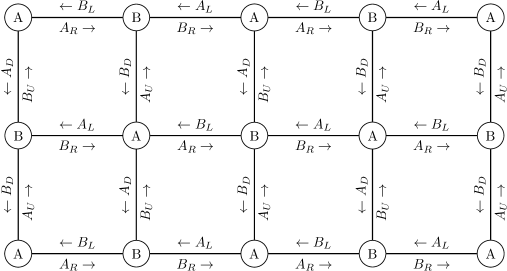
Figure 1: An example of a 2D reducible OQW. The operators are defined in the text. The dashed lines show possible paths from one vertex of type $A$ to another vertex of this type.

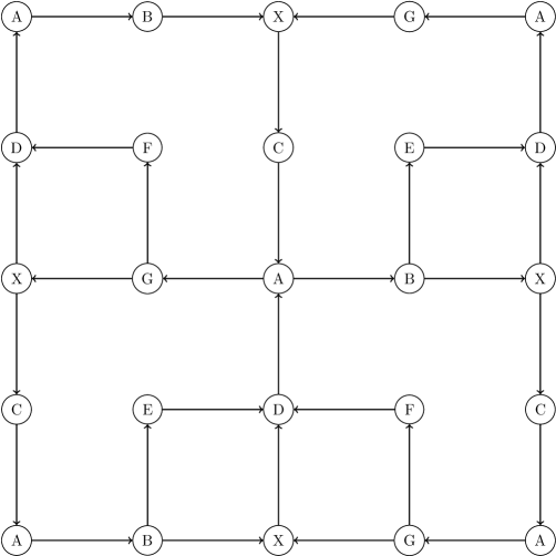
Figure 2: An example of a 2D reducible OQW. The arrows show possible transitions. Each path from one vertex of type $A$ leads to another vertex of this type with exactly 4 steps.

3.1.1 Central limit theorem and its proof

Theorem 2

Consider a reducible open quantum walk on $\mathbb{Z}^{d}$. By $P$ we denote the abstract class of vertices constructed as described in Definition 10. We assume that a channel constructed with these paths $\Phi^{P}$ has a unique invariant state $\rho_{\infty}\in\Omega(\mathcal{X})$ with average transition vector $|m_{P}\rangle$. Let $(\rho_{n},X_{n})_{n\geq 0}$ be the quantum trajectory process associated to this open quantum walk, then

$$\lim_{n\rightarrow\infty}\frac{\mathbb{E}(|X_{n}\rangle)}{n}=|m_{P}\rangle,$$ (24)

and probability distribution of normalized random variable $X_{n}$

$$\frac{|X_{n}\rangle-n|m_{P}\rangle}{\sqrt{n}},$$ (25)

converges in law to the Gaussian distribution in ${\mathbb{R}}^{d}$.

Proof. We apply the Theorem 1 to the reduced OQW as in Def. 10. As all the path’s lengths are equal and describe all possible paths starting from a vertex of type $A$ we have that $\sum_{q=1}^{N}K_{q}^{R\dagger}K_{q}^{R}=\sum_{q=1}^{N}\left(K_{1}^{q}\ldots K_{l}^{q}\right)^{\dagger}K_{1}^{q}\ldots K_{l}^{q}={\rm 1l}_{\mathcal{X}}$. Thus the new walk satisfies assumptions of the Theorem 1. One step of this walk corresponds exactly to $l$ steps of the original walk. The one-to-one correspondence assures that the asymptotic behavior is the same.  

3.1.2 Example

We show the application of Theorem 2 by considering a walk on a network presented in the Fig. 1. The Kraus operators for vertices of type $A$ are defined as follows:

$$\begin{split}A_{U}(X)=&\alpha|0\rangle\langle 0|X|0\rangle\langle 0|+(1-\alpha)|1\rangle\langle 0|X|0\rangle\langle 1|,\\ A_{R}(X)=&\frac{1}{2}|1\rangle\langle 1|X|1\rangle\langle 1|+\frac{1}{2}|3\rangle\langle 1|X|1\rangle\langle 3|\\ A_{D}(X)=&\alpha|3\rangle\langle 2|X|3\rangle\langle 2|+(1-\alpha)|2\rangle\langle 2|X|2\rangle\langle 2|,\\ A_{L}(X)=&\frac{1}{2}|3\rangle\langle 3|X|3\rangle\langle 3|+\frac{1}{2}|0\rangle\langle 3|X|3\rangle\langle 0|.\end{split}$$ (26)

The operators for vertices of type $B$ are:

$$\begin{split}B_{U}(X)=&\alpha|1\rangle\langle 0|X|0\rangle\langle 1|+(1-\alpha)|3\rangle\langle 0|X|0\rangle\langle 3|,\\ B_{R}(X)=&\frac{1}{2}|0\rangle\langle 1|X|1\rangle\langle 0|+\frac{1}{2}|2\rangle\langle 1|X|1\rangle\langle 2|,\\ B_{D}(X)=&\alpha|1\rangle\langle 2|X|2\rangle\langle 1|+(1-\alpha)|3\rangle\langle 2|X|2\rangle\langle 3|,\\ B_{L}(X)=&\frac{1}{2}|0\rangle\langle 3|X|3\rangle\langle 0|+\frac{1}{2}|2\rangle\langle 3|X|3\rangle\langle 2|.\end{split}$$ (27)

In our example we set $\alpha=0.81$. The behavior of this particular walk is presented in Fig. 3. As expected, after a sufficiently large number of steps, the distribution is Gaussian and moves towards the left and down.

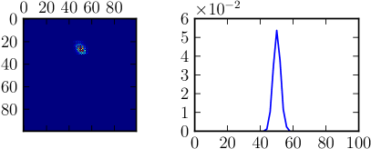
(a)

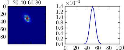
(b)

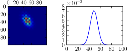
(c)

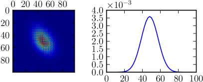
(d)

Figure 3: An example of a reducible OQW on a 2D lattice shown in Fig. 1. The plots show the distribution of the walks for various time steps and a cross section through the center of the distribution. Panel LABEL:sub@fig:reducible-a $n=10$, panel LABEL:sub@fig:reducible-b $n=50$, panel LABEL:sub@fig:reducible-c $n=100$, panel LABEL:sub@fig:reducible-d $n=200$.

3.2 Irreducible OQWs

The assumptions introduced in Theorem 2 allow us to analyze some non-homogeneous OQW, but the class of such walks is still very limited. In this section we aim to provide a way to determine asymptotic behavior of less restricted family of OQWs.

3.2.1 Theorem and proof

Let’s consider an OQW on a network composed with several types of vertices on an infinite lattice. The main assumption of the following theorem is that the distribution of vertex classes is regular over the lattice i.e. density of every vertex class $C\in\Gamma$ is transition invariant.

Definition 11

A regular network is a network where each vertex’s class is assigned randomly at each step with transition invariant probability distribution $\{p_{C}\}_{C}$.

Theorem 3

Given an open quantum walk on $\mathbb{Z}^{d}$ with vertex classes $c(X)\in\Gamma$ for $X\in\mathbb{Z}^{d}$ and associated transition operators $\{K_{1}^{c(X)},\ldots,K_{2d}^{c(X)}\}_{X\in\mathbb{Z}^{d}}\subset L(\mathcal{X})$ we construct for each class of vertices $C\in\Gamma$ a quantum channel $\Phi^{C}$ as in Eq. (21) with a unique invariant state $\rho_{\infty}^{C}\in\Omega(\mathcal{X})$ and an average position vector $|m\rangle=\sum_{C\in\Gamma}p_{C}|m_{C}\rangle$, where $|m_{C}\rangle$ is obtained from Eq. (22) and $p_{C}$ from Def. 11. Let $(\rho_{n},X_{n})_{n\geq 0}$ be the quantum trajectory process associated with this open quantum walk, then

$$\lim_{n\rightarrow\infty}\frac{\mathbb{E}(|X_{n}\rangle)}{n}=|m\rangle,$$ (28)

and probability distribution of normalized random variable $X_{n}$

$$\frac{|X_{n}\rangle-n|m\rangle}{\sqrt{n}},$$ (29)

converges in law to the Gaussian distribution.

Before we prove Theorem 3, let us introduce three technical lemmas.

Lemma 2

For every superoperator $\Phi:L(\mathcal{X})\rightarrow L(\mathcal{X})$ the space $L(\mathcal{X})=\mathrm{Ker}(\Phi)\oplus\mathrm{Im}(\Phi^{\dagger})$.

Proof. First we show that if $A\perp\mathrm{Im}(\Phi^{\dagger})$ then $A\in\mathrm{Ker}(\Phi)$ for $A\in L(\mathcal{X})$. Let us assume $A\perp\mathrm{Im}(\Phi^{\dagger})$. Then for every $B\in L(\mathcal{X})$ it holds that $\mathrm{Tr}(A\Phi^{\dagger}(B))=0$. Then $\mathrm{Tr}(\Phi(A)B)=0$. Thus $\Phi(A)=0$ and $A\in\mathrm{Ker}(\Phi)$.

Now we show that if $A\in\mathrm{Ker}(\Phi)$ then $A\perp\mathrm{Im}(\Phi^{\dagger})$. We assume $\Phi(A)=0$. Then for any chosen $B\in L(\mathcal{X})$ it holds that $\mathrm{Tr}(\Phi(A)B)=0$, thus $\mathrm{Tr}(A\Phi^{\dagger}(B)=0)$, hence $A\perp\mathrm{Im}(\Phi^{\dagger})$.  

Lemma 3

Given a channel $\Phi^{C}$ corresponding to vertex class $C$ with associated Kraus operators $\{K_{1}^{C},\ldots,K_{2d}^{C}\}\subset L(\mathcal{X})$ which has a unique invariant state $\rho_{\infty}$, for every $|l\rangle\in\mathbb{R}^{d}$ there exists $L_{l}^{C}\in L(\mathcal{X})$ such that

$$\left({\rm 1l}_{L(\mathcal{X})}-\left(\Phi^{C}\right)^{\dagger}\right)\left(L_{l}^{C}\right)=\sum_{j=1}^{2d}\left(\left(K_{j}^{C}\right)^{\dagger}K_{j}^{C}\langle{j}|{l}\rangle\right)-\langle{m_{C}}|{l}\rangle{\rm 1l}_{\mathcal{X}}.$$ (30)

Proof. First we compute $\langle{m_{C}}|{l}\rangle$. We get

$$\langle{m_{C}}|{l}\rangle=\sum_{i=1}^{2d}\mathrm{Tr}\left(K_{i}^{C}\rho_{\infty}^{C}\left(K_{i}^{C}\right)^{\dagger}\langle{i}|{l}\rangle\right).$$ (31)

Next, we move all the terms to one side of the equation and write all terms under the trace

$$\sum_{i=1}^{2d}\mathrm{Tr}\left(K_{i}^{C}\rho_{\infty}\left(K_{i}^{C}\right)^{\dagger}\langle{i}|{l}\rangle-\frac{1}{2d}\langle{m_{C}}|{l}\rangle\rho_{\infty}^{C}{\rm 1l}_{\mathcal{X}}\right)=0,$$ (32)

where we multiplied $\langle{m_{C}}|{l}\rangle$ by $\rho_{\infty}^{C}{\rm 1l}_{\mathcal{X}}$. Finally, we use the fact that trace is cyclic and linear and get:

$$\mathrm{Tr}\rho_{\infty}^{C}\left(\sum_{i=1}^{2d}\left(K_{i}^{C}\right)^{\dagger}K_{i}^{C}\langle{i}|{l}\rangle-\frac{1}{2d}\langle{m_{C}}|{l}\rangle{\rm 1l}_{\mathcal{X}}\right)=0.$$ (33)

Thus we obtain that the term under the bracket in Eq. (33) is orthogonal to $\rho_{\infty}^{C}$ and as it is the only invariant state of $\Phi^{C}$ we get that $\mathrm{Ker}({\rm 1l}_{L(\mathcal{X})}-\Phi^{C})=\rho_{\infty}^{C}$. Then, from Lemma 2, the states orthogonal to the kernel are in the image of the conjugated superoperator, hence we get:

$$\sum_{i=1}^{2d}\left(K_{i}^{C}\right)^{\dagger}K_{i}^{C}\langle{i}|{l}\rangle-\frac{1}{2d}\langle{m_{C}}|{l}\rangle{\rm 1l}_{\mathcal{X}}\in\mathrm{Ker}\left({\rm 1l}_{L(\mathcal{X})}-\Phi^{C}\right)^{\perp}=\mathrm{Im}\left({\rm 1l}_{L(\mathcal{X})}-\left(\Phi^{C}\right)^{\dagger}\right).$$ (34)

Hence, we have shown that $L_{l}^{C}$ exists.  

Lemma 4

For each class $C$ and a vector $l\in\mathbb{R}^{d}$ a function

$$f_{C}:\Omega(\mathcal{X})\times\mathbb{R}^{d}\rightarrow\mathbb{R},$$ (35)

given by the explicit formula

$$f_{C}(\rho,i)=\mathrm{Tr}(\rho L_{l}^{C})+\langle{i}|{l}\rangle,$$ (36)

satisfies

$$(1-P_{C})f_{C}(\rho,i)=\langle{i}|{l}\rangle-\langle{m_{C}}|{l}\rangle,$$ (37)

where $P_{C}$ is given by Eq. (20).

Proof. We apply the $P_{C}$ operator as defined in Eq. 20. Let us note that

$$(P_{C}f_{C})(\rho,i)=\sum_{\rho^{\prime},j}P_{C}[(\rho,i),(\rho^{\prime},j)]f_{C}(\rho^{\prime},j).$$ (38)

Applying the definition of $P_{C}$ to (36) we get:

$$\begin{split}(1-P_{C})f_{C}(\rho,i)&=\mathrm{Tr}(\rho L_{l}^{C})+\langle{i}|{l}\rangle-\left[\mathrm{Tr}\left(\sum_{j=1}^{2d}K_{j}^{C}\rho\left(K_{j}^{C}\right)^{\dagger}L_{l}^{C}\right)\right.\\ &+\left.\sum_{j=1}^{2d}\mathrm{Tr}\left(K_{j}^{C}\rho\left(K_{j}^{C}\right)^{\dagger}\right)\langle{j}|{l}\rangle\right].\end{split}$$ (39)

Now, using Lemma 3 we get

$$\mathrm{Tr}\rho\left[\left({\rm 1l}_{L(\mathcal{X})}-\left(\Phi^{C}\right)^{\dagger}\right)\left(L_{l}^{C}\right)-\sum_{j=1}^{2d}\left(K_{j}^{C}\right)^{\dagger}K_{j}^{C}\langle{j}|{l}\rangle\right]+\langle{i}|{l}\rangle=\langle{i}|{l}\rangle-\langle{m_{C}}|{l}\rangle.$$ (40)

which completes the proof.  

Proof of Theorem 3. For a random variable $X_{n}$ we expand the formula $F_{l}=\langle{X_{n}}|{l}\rangle-n\langle{m}|{l}\rangle$:

$$F_{l}=\langle{X_{n}}|{l}\rangle-n\langle{m}|{l}\rangle=\langle{X_{0}}|{l}\rangle+\sum_{k=1}^{n}(\langle X_{k}|-\langle X_{k-1}|)-\langle m|)|l\rangle.$$ (41)

Recall that $\sum_{C\in\Gamma}p_{C}=1$, $m=\sum_{C\in\Gamma}p_{C}m_{C}$ and we denote $\langle X_{k}|-\langle X_{k-1}|=\langle\Delta X_{k}|$, we get:

$$F_{l}=\langle{X_{0}}|{l}\rangle+\sum_{k=1}^{n}\sum_{C\in\Gamma}p_{C}(\langle\Delta X_{k}|-\langle m_{C}|)|l\rangle.$$ (42)

From Lemma 4 we get $(|X\rangle-|m_{C}\rangle)|l\rangle=(1-P_{C})f_{C}(\rho,|X\rangle)$ for some $\rho\in\Omega(\mathcal{X})$, hence:

$$\begin{split}F_{l}&=\langle{X_{0}}|{l}\rangle+\sum_{k=1}^{n}\sum_{C\in\Gamma}p_{C}(1-P_{C})f_{C}(\rho_{k},|\Delta X_{k}\rangle)=\\ &=\langle{X_{0}}|{l}\rangle+\sum_{k=1}^{n}\sum_{C\in\Gamma}p_{C}(f_{C}(\rho_{k},|\Delta X_{k}\rangle)-P_{C}f_{C}(\rho_{k},|\Delta X_{k}\rangle)).\end{split}$$ (43)

After rearranging the sum in the formula for $F_{l}$ we get:

$$\begin{split}F_{l}=&\langle{X_{0}}|{l}\rangle+\sum_{k=2}^{n}\sum_{C\in\Gamma}[p_{C}(f_{C}(\rho_{k},|\Delta X_{k}\rangle)-P_{C}f_{C}(\rho_{k-1},|\Delta X_{k-1}\rangle))]+\\ &+\sum_{C\in\Gamma}p_{C}f_{C}(\rho_{1},|\Delta X_{1}\rangle)-\sum_{C\in\Gamma}p_{C}P_{C}f_{C}(\rho_{n},|\Delta X_{n}\rangle)=M_{n}+R_{n}.\end{split}$$ (44)

Now we consider $M_{n}$ and $R_{n}$ separately. First we discuss $M_{n}$:

$$M_{n}=\sum_{C\in\Gamma}\sum_{k=2}^{n}p_{C}(f_{C}(\rho_{k},|\Delta X_{k}\rangle)-P_{C}f_{C}(\rho_{k-1},|\Delta X_{k-1}\rangle)).$$ (45)

We notice that $M_{n}$ is a centered martingale i.e.

$$\mathbb{E}[\Delta M_{n}|\mathcal{F}_{n-1}]=0,$$ (46)

where $\Delta M_{n}=M_{n}-M_{n-1}$ and $\mathcal{F}$ denotes filtering for stochastic process $M_{n}$ [45, 46]. This follows from the action of $P_{C}$ stated in eq. (38). As $P_{C}$ is a transition operator for the corresponding Markov chain, the value of $P_{C}f_{C}$ for step $k-1$ is exactly the expectation value of $f_{C}$ at the next step

$$\mathbb{E}[f_{C}(\rho_{k},|\Delta X_{k}\rangle)|\mathcal{F}_{k-1}]=P_{C}f_{C}(\rho_{k-1},|\Delta X_{k-1}\rangle).$$ (47)

Additionally $|\Delta M_{n}|$ is bounded from above i.e. $|\Delta M_{n}|<M_{\max}$ as $\Delta M_{n}$ includes terms corresponding to one step of the walk.

In the case of $R_{n}$ we have:

$$R_{n}=\langle{X_{0}}|{l}\rangle+\sum_{C\in\Gamma}p_{C}f_{C}(\rho_{1},|\Delta X_{1}\rangle)-\sum_{C\in\Gamma}p_{C}P_{C}f_{C}(\rho_{n},|\Delta X_{n}\rangle).$$ (48)

From the definition of $f_{C}$ we notice that $R_{n}$ is bounded as the first two terms are constant and the last one $P_{C}f_{C}(\rho,|\Delta X_{n}\rangle)=\mathrm{Tr}(\rho L_{l}^{C})+\langle{\Delta X_{n}}|{l}\rangle$ is clearly bounded, hence$|R_{n}|<R_{\max}$ and $R_{n}$ does not influence the asymptotic behavior.

Now it suffices to show that the following two equalities hold (for proof see Theorem 3.2 and Corollary 3.1 in [46]):

$$\lim_{n\rightarrow\infty}\frac{1}{n}\sum_{k=1}^{n}\mathbb{E}[(\Delta M_{k})^{2}{1}_{|\Delta M_{k}|\geq\epsilon\sqrt{n}}|\mathcal{F}_{k-1}]=0,$$ (49)

and

$$\lim_{n\rightarrow\infty}\frac{1}{n}\sum_{k=1}^{n}\mathbb{E}[(\Delta M_{k})^{2}|\mathcal{F}_{k-1}]=\sigma^{2},$$ (50)

to obtain that $M_{n}/\sqrt{n}$ converges in distribution to $\mathcal{N}(0,\sigma^{2})$, where

$$1_{|\Delta M_{k}|\geq\epsilon\sqrt{n}}=\left\{\begin{matrix}1,{|\Delta M_{k}|\geq\epsilon\sqrt{n}},\\ 0,{|\Delta M_{k}|<\epsilon\sqrt{n}},\end{matrix}\right.$$ (51)

introduces restricted expectation values.

We prove Eq. (49) using the fact that $|\Delta M_{k}|$ is bounded, hence the sum in Eq. (49) terminates for $n>N$, for some $N\in\mathbb{N}$.

In order to prove the equality in Eq. (50) we expand $(\Delta M_{k})^{2}$:

$$\begin{split}(\Delta M_{k})^{2}&=\left(\sum_{C\in\Gamma}p_{C}(\mathrm{Tr}\rho_{k}L_{l}^{C}-\mathrm{Tr}\rho_{k-1}L_{(}\langle\Delta X_{k}|-\langle m_{C}|)|l\rangle)\right)^{2}=\\ &\left(\sum_{C\in\Gamma}p_{C}\Delta M_{k}^{C}\right)^{2}=\sum_{C,C^{\prime}\in\Gamma}p_{C}p_{C^{\prime}}\Delta M_{k}^{C}\Delta M_{k}^{C^{\prime}},\end{split}$$ (52)

where $\Delta M_{k}^{C}=(\mathrm{Tr}(\rho_{k}L_{l}^{C})-\mathrm{Tr}(\rho_{k-1}L_{l}^{C})+(\langle\Delta X_{k}|-\langle m_{C}|)|l\rangle)$. Next, we expand the product

$$\begin{split}\Delta M_{k}^{C}\Delta M_{k}^{C^{\prime}}&=[\mathrm{Tr}(\rho_{k}L_{l}^{C})-\mathrm{Tr}(\rho_{k-1}L_{l}^{C})+(\langle\Delta X_{k}|-\langle m_{C}|)|l\rangle]\times\\ &\times[\mathrm{Tr}(\rho_{k}L_{l}^{C^{\prime}})-\mathrm{Tr}(\rho_{k-1}L_{l}^{C^{\prime}})+(\langle\Delta X_{k}|-\langle m_{C}^{\prime}|)|l\rangle].\end{split}$$ (53)

We divide this expression into three terms $\Delta M_{k}^{C^{\prime}}\Delta M_{k}^{C}=T_{C,C^{\prime}}^{(1,k)}+T_{C,C^{\prime}}^{(2,k)}+T_{C,C^{\prime}}^{(3,k)}$. Henceforth, we will drop indexes $C,C^{\prime},k$ when unambiguous. The term $T^{(1)}$ is equal to:

$$T^{(1)}=\mathrm{Tr}(\rho_{k}L_{l}^{C^{\prime}})\mathrm{Tr}(\rho_{k}L_{l}^{C})-\mathrm{Tr}(\rho_{k-1}L_{l}^{C^{\prime}})\mathrm{Tr}(\rho_{k-1}L_{l}^{C}).$$ (54)

We compute $\mathbb{E}(T^{(1)}|\mathcal{F}_{k-1})$ by adding the term $\pm\mathrm{Tr}(\rho_{k}L_{l}^{C^{\prime}})\mathrm{Tr}(\rho_{k}L_{l}^{C})$

$$\begin{split}\mathbb{E}[T^{(1)}|\mathcal{F}_{k-1}]&=\mathbb{E}(\mathrm{Tr}(\rho_{k}L_{l}^{C^{\prime}})\mathrm{Tr}(\rho_{k}L_{l}^{C})|\mathcal{F}_{k-1})-\mathrm{Tr}(\rho_{k}L_{l}^{C^{\prime}})\mathrm{Tr}(\rho_{k}L_{l}^{C})+\\ &+\mathrm{Tr}(\rho_{k}L_{l}^{C^{\prime}})\mathrm{Tr}(\rho_{k}L_{l}^{C})-\mathrm{Tr}(\rho_{k-1}L_{l}^{C^{\prime}})\mathrm{Tr}(\rho_{k-1}L_{l}^{C}),\end{split}$$ (55)

we obtain a sum of two terms that can be interpreted as an increment part of a martingale and an increment part of a sum respectively. Thus after a summation over $k$ both terms are bounded and we get the equality

$$\lim_{n\rightarrow\infty}\frac{1}{n}\sum_{k=1}^{n}\sum_{C,C^{\prime}\in\Gamma}p_{C}p_{C^{\prime}}\mathbb{E}[T^{(1,k)}_{C,C^{\prime}}|\mathcal{F}_{k-1}]=0.$$ (56)

The term $T^{(2)}$ is given by:

$$T^{(2)}=-\mathrm{Tr}(\rho_{k-1}L_{l}^{C^{\prime}})\Delta M_{k}^{C}-\mathrm{Tr}(\rho_{k-1}L_{l}^{C})\Delta M_{k}^{C^{\prime}}.$$ (57)

We note that $\mathbb{E}(\Delta M_{k}|\mathcal{F}_{k-1})=0$. Thus after summation over $C$ and ${C^{\prime}}$ we get the the expectation value of the whole term $T^{(2,k)}_{C,C^{\prime}}$:

$$\lim_{n\rightarrow\infty}\frac{1}{n}\sum_{k=1}^{n}\sum_{C,C^{\prime}\in\Gamma}p_{C}p_{C^{\prime}}\mathbb{E}[T^{(2,k)}_{C,C^{\prime}}|\mathcal{F}_{k-1}]=0.$$ (58)

We will calculate the term $T^{(3)}$ using the definition of the expectation value. We write the probability of $|\Delta X\rangle$ being equal to $|j\rangle$ and $\rho_{k}$ being $K_{j}\rho_{k-1}K_{j}^{\dagger}/\mathrm{Tr}(A_{j}\rho_{k-1}A_{j}^{\dagger})$ as $\mathrm{Tr}(K_{j}\rho_{k-1}K_{j}^{\dagger})$. This can be expressed in a nice trace form:

$$\begin{split}\mathbb{E}[T^{(3)}_{C,{C^{\prime}}}|\mathcal{F}_{k-1}]&=\mathbb{E}[(\langle\Delta X_{k}|-\langle m_{C}|)|l\rangle(\langle\Delta X_{k}|-\langle m_{C^{\prime}}|)|l\rangle+\\ &+\mathrm{Tr}(\rho_{k}L_{l}^{C^{\prime}})(\langle{\Delta X_{k}}|{l}\rangle-\langle{m_{C}}|{l}\rangle)+\\ &+\mathrm{Tr}(\rho_{k}L_{l}^{C})(\langle{\Delta X_{k}}|{l}\rangle-\langle{m_{C^{\prime}}}|{l}\rangle)|\mathcal{F}_{k-1}]=\\ &=\sum_{i=1}^{2d}\mathrm{Tr}(K_{i}^{c(k-1)}\rho_{k-1}{K_{i}^{c(k-1)\dagger}})\times\\ &\times[(\langle i|-\langle m_{C}|)|l\rangle(\langle i|-\langle m_{C^{\prime}}|)|l\rangle+\\ &+\mathrm{Tr}(K_{i}^{c(k-1)}\rho_{k-1}K_{i}^{c(k-1)\dagger}L_{l}^{C^{\prime}})(\langle{i}|{l}\rangle-\langle{m_{C}}|{l}\rangle)\times\\ &\times\mathrm{Tr}(K_{i}^{c(k-1)}\rho_{k-1}K_{i}^{c(k-1)\dagger}L_{l}^{C})(\langle{i}|{l}\rangle-\langle{m_{C^{\prime}}}|{l}\rangle)],\end{split}$$ (59)

where $c(k-1)$ is the class of $X_{k-1}$. Thus we can define $\Xi_{C,C^{\prime}}^{c(k-1)}$ so that

$$\mathbb{E}[T^{(3)}_{C,C^{\prime}}|\mathcal{F}_{k-1}]=\mathrm{Tr}(\rho_{k-1}\Xi_{C,C^{\prime}}^{c(k-1)}).$$ (60)

After summation over $C$ and $C^{\prime}$ the value is equal to:

$$\lim_{n\rightarrow\infty}\frac{1}{n}\sum_{k=1}^{n}\sum_{C,C^{\prime}\in\Gamma}p_{C}p_{C^{\prime}}\mathbb{E}[T^{(3,k)}_{C,C^{\prime}}|\mathcal{F}_{k-1}]=\lim_{n\rightarrow\infty}\frac{1}{n}\sum_{k=1}^{n}\mathrm{Tr}(\rho_{k-1}\Xi^{c(k-1)}),$$ (61)

where $\Xi^{c(k-1)}=\sum_{C,C^{\prime}\in\Gamma}p_{C}p_{C^{\prime}}\Xi_{C,C^{\prime}}^{c(k-1)}$. By the ergodic theorem (Th. 4.2 in [43]) this converges to:

$$\lim_{n\rightarrow\infty}\frac{1}{n}\sum_{k=1}^{n}\mathrm{Tr}(\rho_{k-1}\Xi^{c(k-1)})=\mathrm{Tr}(\rho_{\infty}\Xi)=\sigma^{2}_{l},$$ (62)

with $\Xi=\sum_{c}p_{c}\Xi^{c}$.

Finally, after summing of all of the terms we get:

$$\lim_{n\rightarrow\infty}\frac{1}{n}\sum_{k}\mathbb{E}[(\Delta M_{k})^{2}|\mathcal{F}_{k-1}]=\sigma_{l}^{2},$$ (63)

which completes the proof.  

3.2.2 Example

As an example of a walk consistent with description in Section 3.2.1 we consider a walk with the same vertex types as in the reducible case, that is:

$$\begin{split}A_{U}(X)=&\alpha|0\rangle\langle 0|X|0\rangle\langle 0|+(1-\alpha)|1\rangle\langle 0|X|0\rangle\langle 1|,\\ A_{R}(X)=&\frac{1}{2}|1\rangle\langle 1|X|1\rangle\langle 1|+\frac{1}{2}|3\rangle\langle 1|X|1\rangle\langle 3|\\ A_{D}(X)=&\alpha|3\rangle\langle 2|X|3\rangle\langle 2|+(1-\alpha)|2\rangle\langle 2|X|2\rangle\langle 2|,\\ A_{L}(X)=&\frac{1}{2}|3\rangle\langle 3|X|3\rangle\langle 3|+\frac{1}{2}|0\rangle\langle 3|X|3\rangle\langle 0|.\end{split}$$ (64)

and

$$\begin{split}B_{U}(X)=&\alpha|1\rangle\langle 0|X|0\rangle\langle 1|+(1-\alpha)|3\rangle\langle 0|X|0\rangle\langle 3|,\\ B_{R}(X)=&\frac{1}{2}|0\rangle\langle 1|X|1\rangle\langle 0|+\frac{1}{2}|2\rangle\langle 1|X|1\rangle\langle 2|,\\ B_{D}(X)=&\alpha|1\rangle\langle 2|X|2\rangle\langle 1|+(1-\alpha)|3\rangle\langle 2|X|2\rangle\langle 3|,\\ B_{L}(X)=&\frac{1}{2}|0\rangle\langle 3|X|3\rangle\langle 0|+\frac{1}{2}|2\rangle\langle 3|X|3\rangle\langle 2|.\end{split}$$ (65)

Although, in this case we assign the type to a vertex randomly with a uniform distribution.

The channels formed from Kraus operators $A_{x}$ and $B_{x}$ where $x\in{U,R,L,D}$ both have a unique invariant state. The behavior of the network is presented in the Fig. 4. We obtain a similar behavior as in the reducible case, although the convergence to a Gaussian distribution is slower.

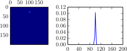
(a)

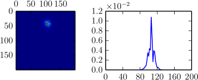
(b)

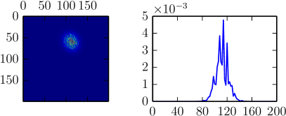
(c)

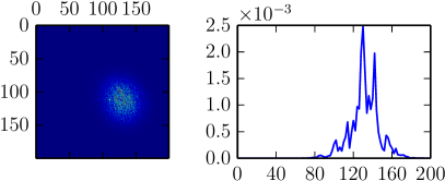
(d)

Figure 4: An example of realization of OQW with a random uniform distribution of vertex types. The figures show the distribution of the walk and cross section through the center for various time steps: panel LABEL:sub@fig:reducible-a $n=10$, panel LABEL:sub@fig:reducible-b $n=100$, panel LABEL:sub@fig:reducible-c $n=200$, panel LABEL:sub@fig:reducible-d $n=500$.

4 Conclusions

The aim of this paper was to provide formulas describing the behavior of the open quantum walk in the asymptotic limit. We described two cases: networks that are reducible to the 1-type case and networks with random, uniformly distributed vertex types. This result allows one to analyze behavior of walks with a more complex structure compared to the known results. We have illustrated our claims with numerical examples that show possible applications and correctness of our theorems. The networks are still restricted to vertices that exhibits invariant states.

We provided examples showing that the theorems are valid in the case of a 2D regular lattice with two vertex types. In Section 3.1.2 we shown application to the reducible case, when the assignment of vertex types is regular and translation invariant. Next, in Section 3.2.2 we turned to a random, uniformly distributed assignment of vertex types.

These theorems can also be applied to the non-lattice graphs. Different types of vertices allow also to apply this in the case of graphs with non-constant degrees. This may be very useful in modeling complex structures, especially of regular definition as in the case of Apollonian networks.

These possibilities are important as open quantum walks with different vertex classes have application in quantum biology and dissipative quantum computing.

References

- [1] S. Attal, F. Petruccione, and I. Sinayskiy, “Open quantum walks on graphs,” Physics Letters A, vol. 376, no. 18, pp. 1545–1548, 2012.
- [2] S. Attal, F. Petruccione, C. Sabot, and I. Sinayskiy, “Open quantum random walks,” Journal of Statistical Physics, vol. 147, no. 4, pp. 832–852, 2012.
- [3] I. Sinayskiy and F. Petruccione, “Open quantum walks: a short introduction,” Journal of Physics: Conference Series, vol. 442, no. 1, p. 012003, 2013.
- [4] R. Sweke, I. Sinayskiy, and F. Petruccione, “Dissipative preparation of generalized bell states,” Journal of Physics B: Atomic, Molecular and Optical Physics, vol. 46, no. 10, p. 104004, 2013.
- [5] I. Sinayskiy and F. Petruccione, “Properties of open quantum walks on ,” Physica Scripta, vol. 2012, no. T151, p. 014077, 2012.
- [6] Ł. Pawela, P. Gawron, J. Miszczak, and P. Sadowski, “Generalized open quantum walks on apollonian networks,” arXiv preprint arXiv:1407.1184, 2014.
- [7] D. Reitzner, D. Nagaj, and V. Buzek, “Quantum walks,” Acta Physica Slovaca, vol. 61, no. 6, pp. 603–725, 2011.
- [8] A. Ambainis, “New developments in quantum algorithms,” Lecture Notes in Computer Science, vol. 6281, pp. 1–11, 2010.
- [9] C. Ampadu, “Limit theorems for quantum walks associated with hadamard matrices,” Physical Review A, vol. 84, no. 1, p. 012324, 2011.
- [10] A. Ahlbrecht et al., “Asymptotic behavior of quantum walks with spatio-temporal coin fluctuations,” Quantum Information Processing, vol. 11, no. 5, pp. 1219–1249, 2012.
- [11] B. Kollar, T. Kiss, J. Novotny, and I. Jex, “Asymptotic dynamics of coined quantum walks on percolation graphs,” Physical Review Letters, vol. 108, p. 230505, 2012.
- [12] L. K. Grover, “Quantum mechanics helps in searching for a needle in a haystack,” Physical Review Letters, vol. 79, no. 2, pp. 325–328, 1997.
- [13] N. Shenvi, J. Kempe, and K. B. Whaley, “Quantum random-walk search algorithm,” Physical Review A, vol. 67, no. 5, p. 052307, 2003.
- [14] R. Portugal, Quantum Walks and Search Algorithms. Quantum Science and Technology, Springer, 2013.
- [15] A. M. Childs and J. Goldstone, “Spatial search by quantum walk,” Physical Review A, vol. 70, no. 2, pp. 022314–1–022314–11, 2004.
- [16] P. Sadowski, “Efficient quantum search on Apollonian networks,” arXiv preprint arXiv:1406.0339, 2014.
- [17] J. A. Miszczak and P. Sadowski, “Quantum network exploration with a faulty sense of direction,” Quantum Information and Computation, vol. 14, no. 13&14, pp. 1238–1250, 2014.
- [18] A. P. Flitney and D. Abbott, “An introduction to quantum game theory,” Fluctuation and Noise Letters, vol. 2, no. 04, pp. R175–R187, 2002.
- [19] E. W. Piotrowski and J. Sładkowski, “An invitation to quantum game theory,” International Journal of Theoretical Physics, vol. 42, no. 5, pp. 1089–1099, 2003.
- [20] Ł. Pawela and J. Sładkowski, “Cooperative quantum parrondo’s games,” Physica D: Nonlinear Phenomena, vol. 256, pp. 51–57, 2013.
- [21] Ł. Pawela and J. Sładkowski, “Quantum prisoner’s dilemma game on hypergraph networks,” Physica A: Statistical Mechanics and its Applications, vol. 392, no. 4, pp. 910–917, 2013.
- [22] M. Dahleh, A. Peirce, and H. Rabitz, “Optimal control of uncertain quantum systems,” Physical Review A, vol. 42, no. 3, p. 1065, 1990.
- [23] L. Viola, S. Lloyd, and E. Knill, “Universal control of decoupled quantum systems,” Physical Review Letters, vol. 83, no. 23, p. 4888, 1999.
- [24] L. Viola and E. Knill, “Robust dynamical decoupling of quantum systems with bounded controls,” Physical Review Letters, vol. 90, no. 3, p. 037901, 2003.
- [25] M. James, “Risk-sensitive optimal control of quantum systems,” Physical Review A, vol. 69, no. 3, p. 032108, 2004.
- [26] C. D’Helon, A. Doherty, M. James, and S. Wilson, “Quantum risk-sensitive control,” in Decision and Control, 2006 45th IEEE Conference on, pp. 3132–3137, 2006.
- [27] D. Dong and I. R. Petersen, “Sliding mode control of quantum systems,” New Journal of Physics, vol. 11, no. 10, p. 105033, 2009.
- [28] Ł. Pawela and Z. Puchała, “Quantum control with spectral constraints,” Quantum Information Processing, vol. 13, no. 2, pp. 227–237, 2014.
- [29] Ł. Pawela and Z. Puchała, “Quantum control robust with respect to coupling with an external environment,” Quantum Information Processing (online first), pp. 1–10, 2014.
- [30] P. Gawron, D. Kurzyk, and Ł. Pawela, “Decoherence effects in the quantum qubit flip game using markovian approximation,” Quantum Information Processing, vol. 13, no. 3, pp. 665–682, 2014.
- [31] Ł. Pawela and P. Sadowski, “Various methods of optimizing control pulses for quantum systems with decoherence,” arXiv preprint arXiv:1310.2109, 2013.
- [32] J. Du, H. Li, X. Xu, M. Shi, J. Wu, X. Zhou, and R. Han, “Experimental realization of quantum games on a quantum computer,” Physical Review Letters, vol. 88, no. 13, p. 137902, 2002.
- [33] A. P. Flitney and D. Abbott, “Quantum games with decoherence,” Journal of Physics A: Mathematical and General, vol. 38, no. 2, p. 449, 2005.
- [34] A. P. Flitney and L. C. Hollenberg, “Multiplayer quantum minority game with decoherence,” Quantum Information & Computation, vol. 7, no. 1, pp. 111–126, 2007.
- [35] Ł. Pawela, P. Gawron, Z. Puchała, and J. Sładkowski, “Enhancing pseudo-telepathy in the magic square game,” PloS one, vol. 8, no. 6, p. e64694, 2013.
- [36] P. Gawron and Ł. Pawela, “Relativistic quantum pseudo-telepathy,” arXiv preprint arXiv:1409.2708, 2014.
- [37] N. Shenvi, K. Brown, and W. K.B., “Effects of a random noisy oracle on search algorithm complexity,” Physical Review A, vol. 68, no. 5, pp. 523131–5231311, 2003.
- [38] J. Lockhart, C. Di Franco, and M. Paternostro, “Performance of continuous time quantum walks under phase damping,” Physics Letters A, vol. 378, p. 338, 2014.
- [39] V. Kendon, “Decoherence in quantum walks - a review,” Mathematical Structures in Computer Science, vol. 17, no. 6, pp. 1169–1220, 2006.
- [40] V. Kendon and B. Tregenna, “Decoherence can be useful in quantum walks,” Pysical Review A, vol. 67, p. 042315, 2003.
- [41] C. Ampadu, “Localization of m-particle quantum walks.” 2011.
- [42] C. M. Chandrashekar, “Decoherence on a two-dimensional quantum walk using four- and two-state particle,” Journal of Physics A, vol. 46, p. 105306, 2013.
- [43] S. Attal, N. Guillotin-Plantard, and C. Sabot, “Central limit theorems for open quantum random walks and quantum measurement records,” in Annales Henri Poincaré, vol. 16, pp. 15–43, Springer, 2014.
- [44] I. Sinayskiy and F. Petruccione, “Open quantum walks: a short introduction,” Journal of Physics.: Conference Series, vol. 442, no. 1, p. 012003, 2013.
- [45] B. M. Brown, “Martingale central limit theorems,” Annals of Mathematical Statistics, vol. 42, pp. 59–66, 02 1971.
- [46] P. Hall and C. Heyde, Martingale Limit Theory and its Applications. Academic Press, 1980.